| Issue |
A&A
Volume 709, May 2026
|
|
|---|---|---|
| Article Number | A86 | |
| Number of page(s) | 10 | |
| Section | Astronomical instrumentation | |
| DOI | https://doi.org/10.1051/0004-6361/202659386 | |
| Published online | 05 May 2026 | |
Electron density estimation from measurements of spacecraft potential using Solar Orbiter
1
Swedish Institute of Space Physics (IRF),
Uppsala
75121,
Sweden
2
Department of Physics and Astronomy, Uppsala University,
Uppsala,
Sweden
3
LIRA, Observatoire de Paris, Université PSL, CNRS, Sorbonne Université, Univ. Paris Cité,
5 place Jules Janssen,
92195
Meudon,
France
4
Radboud Radio Lab, Department of Astrophysics, Radboud University Nijmegen,
The Netherlands
5
Mullard Space Science Laboratory, University College London, Holmbury St. Mary, Dorking,
Surrey
RH5 6NT,
UK
6
Institute of Atmospheric Physics of the Czech Academy of Sciences,
Bocňí II 1a/1401,
14100
Prague,
Czechia
7
Astronomical Institute of the Czech Academy of Sciences,
Bocňí II 1a/1401,
14100
Prague,
Czechia
8
European Space Agency, ESAC, Camino Bajo del Castillo s/n, Urb. Villafranca del Castillo,
28692
Villanueva de la Cañada, Madrid,
Spain
★ Corresponding author: This email address is being protected from spambots. You need JavaScript enabled to view it.
Received:
9
February
2026
Accepted:
16
March
2026
Abstract
Context. Measurements of spacecraft potential (Vsc) are an important tool for plasma diagnostics. High-resolution Vsc measurements can be calibrated with low-cadence observations of electron plasma frequency to derive high-resolution electron density data.
Aims. We analyze Vsc measured by the Radio and Plasma Waves (RPW) instrument suite on board Solar Orbiter. We investigate the evolution of Vsc within the framework of the heliocentric distance and mission lifetime. We aim to obtain electron density estimates that are valid across a wider range of Vsc regimes, including the cases of negative Vsc.
Methods. We determined Vsc by combining measurements of the probe-to-spacecraft potential, Vps, and the probe-to-plasma potential, Vpn. Then, we used the appropriate electric current balance to find a relation between electron density and Vsc, which we calibrated to the observed electron plasma frequency. With this method, we obtained the electron density at the resolution given by the Vps measurements.
Results. We find that Vsc reaches negative values for a larger amount of time than expected for a sunlit spacecraft immersed in a tenuous plasma such as the solar wind. We are now able to identify when these Vsc changes occur, enabling us to estimate the electron density accordingly.
Conclusions. Solar Orbiter charges negatively during periods of high plasma density and low photoelectron emission. However, the measured Vsc is also influenced by the electrical disconnection of the solar arrays from the spacecraft ground during fuse-blowing events. This disconnection raises the local plasma potential near the probes, causing the measured Vsc to appear negative even when Solar Orbiter remains positively charged. By distinguishing between the genuine negative spacecraft charging and the apparent negative charging induced by solar panels, we can refine previous electron density estimation methods to include cases when Vsc < 0 V. This approach provides reliable, high-resolution electron density estimates across both positive and negative Vsc regimes.
Key words: plasmas / space vehicles: instruments / Sun: heliosphere / solar wind
© The Authors 2026
 Open Access article, published by EDP Sciences, under the terms of the Creative Commons Attribution License (https://creativecommons.org/licenses/by/4.0), which permits unrestricted use, distribution, and reproduction in any medium, provided the original work is properly cited.
This article is published in open access under the Subscribe to Open model. This email address is being protected from spambots. You need JavaScript enabled to view it. to support open access publication.
1 Introduction
Spacecraft potential (Vsc) measurements are important for plasma diagnostics (Pedersen 1995; Escoubet et al. 1997; Nakagawa et al. 2000; Pedersen et al. 2008; Ergun et al. 2010; Andriopoulou et al. 2018; Khotyaintsev et al. 2021). A metal object immersed in a plasma will exchange charges with the environment according to the plasma conditions and the object’s properties (Ferguson 2011). Electron collection by the object will increase the buildup of negative charge on the object’s surface, driving its potential negative. On the other hand, the collection of positive ions and electron emission has the opposite effect, where the object’s potential will tend toward positive values.
The exchange of these charges produces electric currents; consequently, for a spacecraft immersed in the solar wind, its electrostatic potential is determined from the following current balance condition,
![Mathematical equation: $\[I_e-I_{p h}-I_i-I_{s e}-I_b+I_{o t h e r}=0,\]$](/articles/aa/full_html/2026/05/aa59386-26/aa59386-26-eq1.png) (1)
(1)
where Ie is the solar wind thermal electron current, Iph is the photoelectron emission current, Ii is the solar wind ion current, Ise is the current from the secondary electrons emitted from the spacecraft, and Iother are other current sources. Furthermore, for a spacecraft equipped with electric field probes, a bias current Ib is often drawn from the spacecraft to the probes. This serves to stabilize the probes at a potential near that of the surrounding plasma.
In a sunlit and tenuous environment such as the solar wind, electron emission usually dominates ion collection (Pedersen et al. 2008). The main contributions to electron emission are photoelectrons and secondary electrons (Diaz-Aguado et al. 2021). By understanding how electron collection and emission work on a spacecraft immersed in the solar wind, we can accurately estimate electron density (ne) and temperature (Te; Escoubet et al. 1997), using the spacecraft’s potential, Vsc, measured by electrostatic probes.
Typical solar wind densities in the inner heliosphere at distances between 0.3 and 1 a.u. range from ~100 to ~102 cm−3 (Marsch & Richter 1984; Verscharen et al. 2019; Khotyaintsev et al. 2021; Kruparova et al. 2023); however, there are instances where the density exceeds these values, for example, in the case of coronal mass ejections (Webb et al. 1993; Trotta et al. 2024, 2025). For typical solar wind densities, the charge transfer between the spacecraft and the solar wind is dominated by the electrons emitted from the spacecraft due to incoming UV and X-Ray photons from the Sun, readily driving the spacecraft’s potential positive. This positive potential draws in more ambient electrons and limits the escape of photoelectrons and secondary electrons, until a balance between the emitted and absorbed charges is reached and the spacecraft “floats” at Vsc.
Using the dependence between Vsc and ne, it is possible to estimate the electron density of a space plasma if a reference electron plasma frequency is known from independent measurements. This method has been applied to many spacecraft to estimate electron density in the near-Earth plasma environment, including ISEE 1 (Escoubet et al. 1997), Geotail (Nakagawa et al. 2000), Polar (Laakso et al. 2002), Cluster (Pedersen et al. 2008), or MMS (Andriopoulou et al. 2018; Graham et al. 2018), as well as (more recently in the solar wind) by Solar Orbiter (Khotyaintsev et al. 2021) and Parker Solar Probe (Mozer et al. 2022). Nevertheless, this method only accounts for positive values of Vsc. For Solar Orbiter, this approach is accurate at the beginning of the mission; at later orbits, the dependence between Vsc and ne becomes more complicated and the method for estimating ne needs to be adjusted.
In this article, we elaborate on the adjustments made to the method developed by Khotyaintsev et al. (2021) to obtain accurate ne values from Vsc under conditions at Solar Orbiter that differ from the ideal scenario. This new method has been developed to be robust for different values of Vsc, especially when Vsc becomes negative. We analyze the evolution of Vsc with mission lifetime and heliocentric distance and discuss its implications for the ne measurements.
We begin by outlining the theoretical background in Sect. 2. In Sect. 3, we introduce the spacecraft potential measurements utilized to develop the ne estimation method and we describe the method in Sect. 4. In Sect. 5, we discuss the Solar Orbiter conditions that lead to the necessity of the new ne estimation method and we present our conclusions in Sect. 6.
2 Theory
The relation between Vsc and ne can be obtained from the current balance condition in Eq. (1). In our convention, the transfer of negative charges from the plasma to the spacecraft results in a positive current, while the transfer of negative charges from the spacecraft to the plasma results in a negative current. The transfer of positive charges from the plasma to the spacecraft also results in a negative current.
Under typical solar wind conditions, Vsc is primarily governed by the balance between Iph and Ie. For the Vsc reached in the solar wind, Iph is usually two orders of magnitude larger than Ii, and even larger closer to the Sun. Consequently, Ii is negligible to a first approximation in the solar wind (Pedersen et al. 2008; Diaz-Aguado et al. 2021) and only becomes significant when Vsc reaches large negative values, as in planetary ionospheres (Hoegy & Wharton 1971; Krehbiel et al. 2007). Secondary electrons can become important during intervals of enhanced flux of high-energy electrons. We discuss the effect of secondary electrons on the ne estimation in Sect. 5. Furthermore, Iother values are assumed to be negligible.
The functional form of the different current contributions varies depending on the Vsc regime. When Vsc is positive, ambient electrons will be attracted. The solar wind thermal electron current increases with increasing Vsc and depends on electron temperature, Te. In the case of a spherical body of a surface area, S, and size around the Debye length (![Mathematical equation: $\[\lambda_{D e}=\sqrt{\epsilon_{0} \kappa_{B} T_{e} / q^{2} n_{e}}\]$](/articles/aa/full_html/2026/05/aa59386-26/aa59386-26-eq2.png) ) or smaller, the ambient solar wind thermal electron current (Mott-Smith & Langmuir 1926; Laframboise & Parker 1973; Pedersen 1995) is given by
) or smaller, the ambient solar wind thermal electron current (Mott-Smith & Langmuir 1926; Laframboise & Parker 1973; Pedersen 1995) is given by
![Mathematical equation: $\[I_e=S ~q n_e \sqrt{\kappa_B T_e / 2 \pi m_e}\left(1+q V_{s c} / \kappa_B T_e\right),\]$](/articles/aa/full_html/2026/05/aa59386-26/aa59386-26-eq3.png) (2)
(2)
where ϵ0 is the permittivity of free space, κB is the Boltzmann constant, and q and me are the electron charge and mass, respectively.
The emitted photoelectrons will be attracted back to the surface of the spacecraft, reducing Iph from its maximum value, the photosaturation current Iph0 = Sph Jph0. Here, Sph is the spacecraft’s sunlit area and Jph0 is the photosaturation current density. Under the assumption of a Maxwellian distribution of photoelectrons, the decrease in Iph with Vsc is described by an exponential with e-folding energy related to the photoelectron temperature Tph (Grard 1973), as
![Mathematical equation: $\[I_{p h}=S_{p h} J_{p h 0} e^{-q V_{s c / \kappa B} T_{p h}}.\]$](/articles/aa/full_html/2026/05/aa59386-26/aa59386-26-eq4.png) (3)
(3)
We note that in the presence of strong external electric fields, such as during periods of strong wave activity, photoelectron escape can be enhanced, altering this relation between Vsc and Iph (Torkar et al. 2017; Graham et al. 2018). In the solar wind, these instances are uncommon and are typically restricted to periods when the source regions of intense radio bursts are being directly observed (Gurnett & Anderson 1977).
Combining Eqs. (2) and (3), we obtained the current balance for a positively charged spacecraft,
![Mathematical equation: $\[S_{p h} J_{p h 0} e^{-q V_{s c} / \kappa_B T_{p h}}=S ~q n_e \sqrt{\kappa_B T_e / 2 \pi m_e}\left(1+q V_{s c} / \kappa_B T_e\right).\]$](/articles/aa/full_html/2026/05/aa59386-26/aa59386-26-eq5.png) (4)
(4)
If Vsc ≪ κBTe, the last term in the right-hand side of Eq. (4) can be neglected. In that case, Vsc (Salem et al. 2001; Ergun et al. 2010) is given by
![Mathematical equation: $\[V_{s c}=\frac{\kappa_B T_{p h}}{q} ln \left(\frac{S_{p h}}{S} \frac{J_{p h 0}}{n_e q \sqrt{\kappa_b T_e / 2 \pi m_e}}\right).\]$](/articles/aa/full_html/2026/05/aa59386-26/aa59386-26-eq6.png) (5)
(5)
In Sect. 5, we address the implications for cases, where the condition Vsc ≪ κBTe is not satisfied. Rearranging Eq. (5), we get the following expression for ne,
![Mathematical equation: $\[n_e=\frac{S_{p h}}{S} \frac{J_{p h 0}}{q \sqrt{\kappa_B T_e / 2 \pi m_e}} e^{-q V_{s c} / \kappa_B T_{p h}}.\]$](/articles/aa/full_html/2026/05/aa59386-26/aa59386-26-eq7.png) (6)
(6)
When Vsc < 0 V, the solar wind electrons are repelled and only the ones with sufficient energy will reach the spacecraft body. In this scenario, Ie will decrease exponentially since a larger number of electrons are repelled as Vsc becomes more negative (Mott-Smith & Langmuir 1926), given by
![Mathematical equation: $\[I_e=S ~q n_e \sqrt{\kappa_B T_e / 2 \pi m_e} e^{q V_{s c} / \kappa_B T_e}.\]$](/articles/aa/full_html/2026/05/aa59386-26/aa59386-26-eq8.png) (7)
(7)
In contrast, since all the emitted electrons will also be repelled, Iph will be equal to its maximum value for the given photon flux
![Mathematical equation: $\[I_{p h}=S_{p h} J_{p h 0} \equiv I_{p h 0}.\]$](/articles/aa/full_html/2026/05/aa59386-26/aa59386-26-eq9.png) (8)
(8)
The current balance for Vsc < 0 V yields
![Mathematical equation: $\[S_{p h} J_{p h 0}=S ~q n_e \sqrt{\kappa_B T_e / 2 \pi m_e} e^{q V_{s c / \kappa_B T_e}},\]$](/articles/aa/full_html/2026/05/aa59386-26/aa59386-26-eq10.png) (9)
(9)
and Vsc is
![Mathematical equation: $\[V_{s c}=\frac{\kappa_B T_e}{q} ln \left(\frac{S_{p h}}{S} \frac{J_{p h 0}}{n_e q \sqrt{\kappa_b T_e / 2 \pi m_e}}\right).\]$](/articles/aa/full_html/2026/05/aa59386-26/aa59386-26-eq11.png) (10)
(10)
Again, rearranging to express ne as a function of Vsc we get
![Mathematical equation: $\[n_e=\frac{S_{p h}}{S} \frac{J_{p h 0}}{q \sqrt{\kappa_B T_e / 2 \pi m_e}} e^{-q V_{s c} / \kappa_B T_e}.\]$](/articles/aa/full_html/2026/05/aa59386-26/aa59386-26-eq12.png) (11)
(11)
Although similar in form, Eqs. (6) and (11) show a different relation between ne and Vsc. Specifically, ne is a function of Tph in Eq. (6) and a function of Te in Eq. (11). The rearrangement of ne as a function of Vsc allows us to group the various parameters into two calibration constants n0 and β. We can then rewrite the equations as ne = n0e−Vsc/β. In this way, the accuracy of our density estimation method does not have to rely on the knowledge of every parameter in Eqs. (6) and (11). Instead, we we fit the parameters n0 and β over short time intervals, as detailed in Sect. 4.
3 Spacecraft potential measurements
The Radio and Plasma Waves (RPW) instrument suite (Maksimovic et al. 2020) on board Solar Orbiter has three electric-field probes, each consisting of a 6.5 m cylindrical monopole antenna mounted on a 1 m boom. The configuration of these probes is sketched in Fig. 1a. The three antennas lie in a plane perpendicular to the direction between the Sun and the spacecraft. The electrostatic potential between each probe and the spacecraft (Vps) is measured continuously with a typical cadence of 16 Hz. There are also intervals during which cadence is increased to 256 Hz or 4096 Hz.
The characteristic timescale for a spacecraft to reach current balance through charging or discharging is defined by the time constant, τ = RshCsh, where Rsh and Csh represent the resistance and capacitance of the spacecraft’s electrostatic sheath, respectively. Based on Solar Orbiter’s geometry and material properties, the sheath resistance is approximately 5 · 105 Ω and its capacitance is roughly 200 pF, in a low density environment (2 cm−3). These values give a characteristic charging timescale of τ ≈ 0.1 ms.
In higher density regions, sheath resistance decreases, while capacitance stays relatively constant; hence, the charging time decreases further to the order of μs. Consequently, current balance is achieved significantly faster than the typical sampling rate of probe potential measurements. Only the highest resolution data, sampled at Δt ≈ 0.25 ms, could potentially be affected by these sheath dynamics at low density environments.
The actual Vsc is not directly measured as the antennas do not reach infinity. However, a fraction of Vsc is sampled by Vps as illustrated in Fig. 1b for Vsc ≥ 0 V and in Fig. 1c for Vsc < 0 V. In panels b and c the dashed blue line depicts the electrostatic potential of the spacecraft in the absence of the probes and with respect to the electrostatic potential of the ambient solar wind at infinity V0. At the spacecraft surface, the value of the spacecraft potential is Vsc and decreases with distance from the spacecraft body. The rate at which the spacecraft potential decreases depends on λDe. The voltage difference between the spacecraft surface and the solar wind at infinity is not directly known because a probe at infinity is not available. Nevertheless, if Vsc drops with distance quickly enough, the probes can be considered effectively at infinity. In practice, the probes are located relatively close to the spacecraft and measure only a fraction of the total potential drop; they are at a voltage, Vn0, above or below the solar wind, depending on the polarity of Vsc.
Moreover, just as with the spacecraft, the probes are immersed in the plasma themselves and they also develop an electrostatic potential surrounding them. The red curves in panels b and c illustrate the potential profile only of the antennas with respect to V0. The potential between the probe and the plasma surrounding it Vpn is driven to ~1 to 2 V by a bias current (Ib). The current balance of the probes is then
![Mathematical equation: $\[I_e+I_b=I_{p h}.\]$](/articles/aa/full_html/2026/05/aa59386-26/aa59386-26-eq13.png) (12)
(12)
Because of the development of the probe potential, the antennas are not simply at the spacecraft potential value at the probe location, Vn0. Instead, they are driven at a voltage, Vn0 + Vpn, from V0 (or, equivalently, at Vsp volts from Vsc).
The total electrostatic potential profile, including the spacecraft and antenna potentials, is illustrated by the yellow curves in panels b and c. We note that Vps is measured from the probe to the spacecraft; therefore its contribution is opposite in sign to Vsc. The total Vsc can be expressed as
![Mathematical equation: $\[V_{s c}=-V_{p s}+V_{p n}+V_{n 0}.\]$](/articles/aa/full_html/2026/05/aa59386-26/aa59386-26-eq14.png) (13)
(13)
The final potential drop from the plasma near the probe and the solar wind, Vn0, is unknown, but it is accounted for by considering it a fraction of the total Vsc (Pedersen et al. 2008). Then, we can rewrite Eq. (13) in terms of a factor α of the RPW measurements via
![Mathematical equation: $\[V_{s c}=\alpha\left(V_{p n}-V_{p s}\right).\]$](/articles/aa/full_html/2026/05/aa59386-26/aa59386-26-eq15.png) (14)
(14)
To obtain Vpn, we use the current sweeps performed once a day by RPW. In the I–V (current-voltage) curve, as the one shown in Fig. 2, the voltage values for each current setting are shown. As Ib is changed, the probe will develop a different voltage with respect to the surrounding plasma. Since the only directly measured potential is Vps, the x-axis of the I–V curve represents this quantity. To the left of the I–V curve, toward more negative Vps, the probe is negative with respect to the near plasma. In this regime, most solar wind electrons are repelled, and all the photoelectrons escape. At this point, the current reaches the photosaturation value. As Ib is increased, the potential is driven toward positive values and more solar wind electrons are absorbed. Once the potential of the probe changes to positive, Iph0 is exponentially reduced and Ie increases according to Eq. (2).
At the boundary of the I–V curve between the electron retarding region (where the current is constant) and the electron attracting region (where the current is nearly exponential), the probe potential flips sign. The Vps value in the I–V curve at this boundary corresponds to the probe being at the same potential as the surrounding plasma. If the sheath of the spacecraft is small, the surrounding plasma will be the unperturbed solar wind. Usually, the sheath of the spacecraft extends beyond the probe. Finally, to get Vpn, we subtract the Vps value at the I–V boundary from the Vps at Ib, which is simply the operating voltage Vps, depicted by the red dot in Fig. 2. Once the daily Vpn is retrieved, it is interpolated to the Vps resolution.
After calculating all the potentials, we obtained Vsc using Eq. (14). We assumed α = 1.5, which was empirically determined based on data from the beginning of the mission. However, as we demonstrate in Sect. 5, this value changes over the course of the mission. In Figs. 3a and 3c, we plot Solar Orbiter’s Vsc against mission lifetime and heliocentric distance (R), respectively.
To avoid issues related to solar cell strings short-circuiting the solar panel structure (e.g. due to micrometeroid impacts), the design of the solar panels required us to connect the panel structures to the spacecraft ground through resistors (on the order of tens of kΩ). While this minimizes undesirable currents, we realized that it would allow the solar panels to float to an unknown voltage with respect to the spacecraft. Consequently, this could cause an uncontrolled perturbation to the DC electric field measurements. Therefore, hard ground connections through fuses were provided in parallel to the resistors. As long as no other issues appeared in the solar panels, they were kept at Vsc, providing a symmetric electrostatic field around the spacecraft, which is advantageous for E-field measurements.
The ratio of the total area to photoemitting area S/Sph of a flat solar panel is ~ 2, while for the approximately cube-shaped spacecraft is ~ 6. This means that the Vsc becomes more positive as long as the fuses are intact (cf. Eq. (5)). The vertical green lines in the top panels of Fig. 3 indicate the identified events when fuses have blown. In panel a, we see consistently positive Vsc values in the initial part of the mission, with more excursions to negative potential as one after another of the six solar panels became disconnected by fuse events. Panel b depicts the percentage of data points per month for which Vsc ≥ 0 V.
Notably, Vsc remains mostly positive at the beginning of the mission, with minor decreases at perihelia, where the effective area emitting photoelectrons decreases because the solar panels are not kept orthogonal to the Sun’s direction. After the solar array fuse events, the correlation between the percentage of time at positive potential and R is reversed. This is clearest during 2022 when aphelion was still at ~1 au, but the perihelion was lowered to ~0.3 au. After this reduction of perihelion, Vsc < 0 V for extended periods.
Although negative Vsc can occur due to specific solar wind conditions, measurements are also influenced by the electrostatic floating potential of the solar arrays, VSA. This potential can extend toward the antennas, effectively increasing the potential of the surrounding plasma. If this near-probe plasma potential exceeds Vsc, the measured Vps value will be positive, resulting in a negative Vsc calculation, following Eq. (14), even if the spacecraft itself remains positively charged. Consequently, not all periods of measured Vsc < 0 V shown in Figs. 3a and b are driven by the physical charging of the spacecraft, as some might result from VSA interference. While disentangling these effects requires knowledge of the complex interaction of the spacecraft and solar arrays’ electrostatic environments, we can empirically distinguish between true and apparent negative Vsc. This is achieved by identifying changes in the relation between ne and Vsc, a distinction that is intrinsically integrated into our ne estimation method.
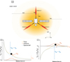 |
Fig. 1 Schematic of Solar Orbiter’s electrostatic potential. (a) Simplified description of the electrostatic potential formed around the spacecraft body (yellow) and the three antennas (red). The color gradient indicates that the potentials decay with distance. For simplicity, the electrostatic potential is depicted as symmetrical and spherical around the spacecraft and the antennas, which is not necessarily the case. Furthermore, it changes with mission lifetime and solar wind conditions. (b) Spacecraft potential profile with respect to distance from the spacecraft surface along the axis of one of the antennas for the case when Vsc ≥ 0 V (dashed blue curve). Similarly, antennas (solid black circle) develop an electrostatic potential that decreases with distance from their surface (red curve). The total potential profile is the superposition of the antenna and spacecraft potentials (yellow). The total Vsc is the sum of the potential drop between the spacecraft surface and the probe (Vsp = −Vps), the potential drop between the probe and the surrounding plasma (Vpn), which is the plasma influenced by the spacecraft sheath at the antenna location, and the potential drop between the plasma surrounding the probe and the unperturbed solar wind (Vn0). (c) Same as in panel (b), but for the case where Vsc < 0 V. |
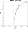 |
Fig. 2 Example of an I-V curve from a current sweep performed by the Solar Orbiter RPW instrument with antenna 1. The red dot indicates the operating potential, which is the potential at which the antenna floats with the programmed bias current commanded between sweeps. The knee of the I–V marked with a dashed green vertical line indicates the Vps, where the probe switches from negative to positive potential. The potential difference between the operating voltage (Vps) and the knee of the I–V curve (dashed green line) is the probe-to-near plasma potential (Vpn). |
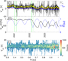 |
Fig. 3 Overview of Solar Orbiter Vsc. (a) Evolution of the spacecraft potential determined from Eq. (14). The yellow line depicts the smoothed Vsc showing its average trend. Similarly, the solid blue line represents the smoothed spacecraft-to-probe potential −Vps = Vsp. (b) Percentage of data points within a month where Vsc ≥ 0 V. The right axis shows Solar Orbiter’s heliocentric distance in au. Most of the time the potential is positive, but there are moments where it becomes negative. The green vertical lines mark the times of the discrete events related to the solar array fuses. (c) Histogram of Vsc with heliocentric distance. |
4 Double-fit density estimation
The density estimation method presented here is an extension of the approach previously developed by Khotyaintsev et al. (2021) to include times when Vsc < 0 V. We define the parameter n0 by grouping all terms in the coefficient of Eqs. (6) and (11) as
![Mathematical equation: $\[n_0=\frac{S_{p h}}{S} \frac{J_{p h 0}}{q \sqrt{2 \pi m_e / \kappa_B T_e}},\]$](/articles/aa/full_html/2026/05/aa59386-26/aa59386-26-eq16.png) (15)
(15)
and from the corresponding exponents we define the parameter β* as
![Mathematical equation: $\[\beta_*=\kappa_B T_* / q.\]$](/articles/aa/full_html/2026/05/aa59386-26/aa59386-26-eq17.png) (16)
(16)
The * indicates ph for photoelectrons and e for solar wind electrons. Since the only high-resolution voltage measurement is for Vps, we can use this to estimate ne by rewriting Eqs. (6) and (11) as
![Mathematical equation: $\[n_e=n_0 e^{V_{p s} / \beta_*}.\]$](/articles/aa/full_html/2026/05/aa59386-26/aa59386-26-eq18.png) (17)
(17)
To determine n0 and β*, we performed a standard linear regression to fit Vps as a function of the natural logarithm of a reference ne. This reference is taken from low-cadence, non-continuous, plasma frequency data nTNR, obtained from the RPW’s Thermal Noise Receiver (TNR; Maksimovic et al. 2020, 2021) using quasi-thermal noise (QTN) spectroscopy. An example of the TNR dynamic spectra and the identified nTNR is shown in Fig. 4a. The vertical axis of the spectrogram corresponds to the frequency of the antenna 1 and antenna 2 dipole signal. The enhanced signature between ~50–80 kHz is the electron plasma frequency fpe, commonly referred to as the plasma line. The red dots correspond to the retrieved nTNR = (fpe/8.980)2, where nTNR is in cm−3 and fpe in kHz.
In general, using QTN to obtain the reference ne produces accurate results. Nevertheless, some limitations may increase the uncertainties of the nTNR and (by extension) the ne using Vps. First, when the antenna length is much shorter than λDe, the plasma line is fainter and cannot be resolved (Meyer-Vernet et al. 2017). In these situations, it is not possible to retrieve nTNR, reducing the efficacy of the fit. This occurs for tenuous and cold plasmas. Also, at these low ne values, the power of the signal noise can get higher than the fpe signal. Typically, the cutoff to obtain nTNR with RPW is around 2 cm−3; below this value, the accuracy of the fit is reduced due to the lack of reference nTNR points. Similarly, fpe identification from TNR measurements is restricted to frequencies below ~100 kHz, corresponding to 125 cm−3, due to strong electromagnetic interference at higher frequencies. Finally, the discretization of the TNR frequency bins introduces an uncertainty δnTNR/nTNR of around ~8.6% (Maksimovic et al. 2021).
To perform the fit, Vps is downsampled to the nTNR resolution. An example of the downsampled Vps fit with ln(nTNR) is presented in Fig. 5. This example fit was taken from 2021-08-12T00:00:00 to 2021-08-29T20:00:00. Furthermore, the use of Vps is justified because we performed a linear fit with the natural logarithm of nTNR, so any difference of Vps from Vsc due to Vpn is accounted for by n0 and differences due to α are accounted for within β*.
To avoid errors in the fit that may arise from changes in n0 and β* we manually selected appropriate time intervals, where Te, Iph0, Vpn, and S/Sph (due to the rotating solar arrays) do not change significantly. These intervals depend on solar wind conditions and heliocentric distance and can last a few months to less than a day. Nonetheless, the interval must contain sufficient data points to perform a reliable fit. In practice, we require at least a few tens of data points for the whole time interval and more than five Vsc data points at each nTNR value.
For intervals where Vsc does not change sign, the relation between ln(nTNR) and Vps is a single linear fit. However, in the example shown in Fig. 5, the slope changes around 0.5 V, indicating a sign change of the spacecraft potential. A single fit cannot be performed and both relations in Eqs. (6) and (11) need to be considered. Values below the point where the slope changes correspond to positive Vsc and the slope is given by β* = βph. The upper part corresponds to negative Vsc and β* = βe. By dividing a single interval into two distinct fits based on the polarity of Vsc, we can estimate the density without having to reduce the interval time and thus getting fewer data points, reducing the accuracy of the fit.
Furthermore, provided that Vsc maintains the same polarity for a duration sufficient to capture enough nTNR reference points, the single-fit method can still be implemented using either Eq. (6) or (11), as appropriate. Performing the calibration fit within a single Vsc regime yields the same results as when the double-fit is applied, but it keeps the calibration procedure simpler. In practice, however, the number of reference points available during intervals of Vsc < 0 V is substantially lower than during periods of Vsc ≥ 0V. As a consequence, the single-fit is typically restricted to cases where Vsc is positive.
Once the fit is performed on the selected interval and the parameters n0 and β* are determined, the data points that lie ±1 V away from the fit are labeled as outliers. Then, a final fit is performed without the outliers. The outlier points are plotted with red dots in Fig. 5. Next, we use Eq. (17) to get ne data at the cadence of the high-resolution Vps measurements. The parameter βph is used when Vsc ≥ 0 and βe when Vsc < 0. Figure 4b shows the density estimation for a portion of the example interval in Fig. 5. The black curve corresponds to the double-fit method, and the reference nTNR data points are presented with red circles. The blue curve, corresponds to the single-fit method, which does not account for the change in slope in the Vps − ln(nTNR) relation. In panel c, the residual values from both fits, calculated as (nTNR − ne)/ne × 100, are shown. The double-fit estimate provides more accurate ne results than the single-fit, especially at higher densities.
The ne estimated by the two-fit method using RPW measurements yields accurate data at a high resolution. Especially, the two-fit method improves the estimation of the single fit at higher densities. At the moment of writing this article, these data are available as an L3 product (solo_13_rpw-bia-density) at the Solar Orbiter archive up to April 2025, with a gap between August 2023 and February 2025. More data are calibrated as new reference nTNR measurements are retrieved.
Data prior to 2021 were calibrated using the one-fit method described in Khotyaintsev et al. (2021) because Vsc was rarely negative and the updated method was not necessary. Since 2021, the double-fit method presented here has been used to provide RPW ne data. The datasets include quality flags to identify intervals where nTNR cannot be reliably retrieved; namely, at high (≳120 cm−3) and low (≲2 cm−3) densities. Details regarding quality flags and data usage are available at the RPW Data Center1.
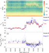 |
Fig. 4 Example of RPW measurements and ne estimation. (a) Dynamic spectra of the antenna 1 and antenna 2 voltage signal. The plasma line, corresponding to fpe is visible as the enhanced signal between ~50–80 kHz. The red dots correspond to the low-cadence, non-continuous reference nTNR (b) Density estimated using calibration method of RPW data (black). The fit is used based on TNR plasma line detection (red circles). For comparison, we show the resulting ne from the single-fit estimation (blue), which does not account for the change in slope of the Vps − ln(nTNR) relationship. (c) Residual values (nTNR − ne)/ne × 100 of the double-fit (black) and single-fit (blue) estimation methods. This example corresponds to a section of the calibration interval in Fig. 5. |
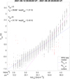 |
Fig. 5 Example of a density calibration interval. The probe-to-spacecraft potential Vps is plotted against low cadence density nTNR determined by TNR plasma line measurements (black dots). The median for each nTNR value is indicated by magenta circles. Points at a distance ±1 V from the median are marked as outliers (red dots). If Vsc does not change sign, a linear relation is expected. If Vsc changes sign, two linear fits are required (blue and pink). |
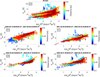 |
Fig. 6 nTNR vs. Vps. (a) All data points from 2020-06-15 to 2023-08-31. (b) Data points from first to second perihelion. (c) Data points from the second to fourth perihelion. (d) Data from the fourth the fifth perihelion. (e) Data from the fifth perihelion to approximately one month before the sixth perihelion. Color code indicates distance from the Sun R in au. |
4.1 Orbital trends
In Fig. 6, we plot all the nTNR against the downsampled Vps up to September 2023. The color code indicates R in au. We multiply ne by R2 to eliminate the radial dependence, which allows a better visualization of the evolution of β*. In Fig. 6a, we see that the behavior of the measurements changes, as seen from the different data populations. These different clusters of points are a product of the Vsc–ne relation, at a given R, evolving with the mission lifetime.
In panels b–e, we separated the data for different time intervals with similar Vsc-ne behavior. For the first interval in panel b, Vsc is mostly positive, and the slope of the data is basically constant for every R. This is because over this interval β* = βph. Over the other intervals in panels c–e, when the Vsc reaches negative values, the upper part of the plot does not present a constant slope for all R. At this point β* = βe, and this change in slope at larger Vps corresponds to different Te values. We note that we chose to plot ln(nTNR) in the x-axis, so an increasing slope means a higher Te. We see that Te increases as Solar Orbiter gets closer to the Sun, while Tph, corresponding to the slope of the lower part of the plots, remains mostly constant.
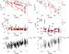 |
Fig. 7 Calibration parameters from the double-fit calibration method (red) and calibration parameters after correcting for the Vps fit (black). Each data point corresponds to a calibration parameter for a given calibration interval. (a) n0 for Vsc ≥ 0V. (b) n0 for Vsc < 0V. (c) βph, corresponding to Tph for Vsc ≥ 0V. (d) βe, corresponding to Te, for Vsc < 0V. Blue dots indicate electron temperature from EAS. (e) Median value of the α parameter determined from Eq. (21) considering Vsc ≥ 0 V for each calibration interval. (f) Median value of the α parameter determined from Eq. (21) considering Vsc < 0 V for all calibration intervals that require two fits. The error bars are calculated from the standard deviation of α values in each interval. |
4.2 Calibration parameters
We applied the double-fit method for the estimation intervals where Vsc remains negative long enough to modify the slope of the Vps-ln(nTNR) relationship, such as in the example interval shown in Fig. 5. Figure 7 displays the calibration parameters n0 and β* as a function of R for all calibration intervals through September 2023. Here, the red points represent parameters derived directly from the Vps–ln(nTNR) fit. Because we fit Vps (rather than Vsc), a correction is required to interpret the physical meaning of the calibration parameters. The correction is achieved by substituting Vps for Vsc in Eqs. (6) and (11), using the expression of Vsc given by Eq. (14). The correction for β* yields
![Mathematical equation: $\[\beta_{corr, *}=\alpha \beta_*.\]$](/articles/aa/full_html/2026/05/aa59386-26/aa59386-26-eq19.png) (18)
(18)
Similarly, the correction for n0 is
![Mathematical equation: $\[n_{0, corr}=n_0 e^{V_{p n} / \beta_*}.\]$](/articles/aa/full_html/2026/05/aa59386-26/aa59386-26-eq20.png) (19)
(19)
The corrected parameters are plotted with black dots in Fig. 7. To estimate α, we assume the voltage relation with distance from the spacecraft body, r (Graham et al. 2018) as
![Mathematical equation: $\[V(r)=\frac{V_{s c} R_0}{r} e^{-\frac{\left(r-R_0\right)}{\Lambda_{D e}}},\]$](/articles/aa/full_html/2026/05/aa59386-26/aa59386-26-eq21.png) (20)
(20)
where R0 is the length of the spacecraft along the direction r, and r ≥ R0. Using again the expression of Vsc given by Eq. (14) and solving at the antenna location, r = Lant, the following expression for α is obtained,
![Mathematical equation: $\[\alpha=\frac{1}{1-\frac{R_0}{L_{a n t}} e^{-\frac{L_{a n t}-R_0}{\lambda_{D e}}}}.\]$](/articles/aa/full_html/2026/05/aa59386-26/aa59386-26-eq22.png) (21)
(21)
The value of α is around 1.5 when Vsc is positive. When Vsc is negative, the influence of the solar arrays becomes important because their contribution to the near-probe potential opposes Vsc. In this regime, determining α requires an assumption about VSA, leading to greater uncertainties in both α and the corrected calibration parameters. If we consider the fact that the dominant current on the solar arrays is the current delivered to the spacecraft, we can assume VSA ≈ 40 V. By applying the voltage profile defined in Eq. (20) and superimposing it onto Vsc, a range of α values between ~3–6 are obtained.
With the α values obtained, we can correct the calibration parameters using Eqs. (18) and (19). The corrected calibration parameters are shown with black dots in Fig. 7. The median α values for each calibration interval obtained from Eq. (21) are shown in panels e and f, considering positive and negative Vsc, respectively.
Figure 7a shows the parameter n0, which decreases with increasing R, as expected since it depends on Iph0. It has units of number density and is related to the density required for the spacecraft to float at 0 V. However, this is not the actual ne value, since the spacecraft is usually not floating at 0 V. The extreme cases are likely due to time intervals where the density or UV flux were unusually low or high for the given R.
Moreover, the set of points with lower values corresponds to the later stages of the mission, when the solar panels where already floating independently from the spacecraft. These data points at lower n0 signify that in order to drive Vsc = 0 V, a lower density is needed. This is because the solar panels are no longer connected to the spacecraft ground and Vsc is reduced through the increase in the S/Sph ratio, as described by Eq. (5). In contrast, at closer R, the larger Iph0 readily drives Vsc to be positive. This behavior is also reflected in Fig. 3b, where the fraction of time where Vsc < 0 V is reduced at perihelia and increased at aphelia after the solar arrays fuse events. Similar results for n0 are obtained from the calibration when Vsc < 0 V, as shown in panel d.
The uncorrected βph parameter, shown with the red dots in Fig. 7c, exhibits a nearly constant behavior with a mean value around 1.5 eV. The corrected βph, corresponding to Tph in eV, has mean value around 2 eV. The error bars are taken from the variations of the estimation of α within a calibration interval and do not include any error on the actual fit. We note that there are a few outlier points, which may arise from uncertainties in the fit, high secondary electron currents, overly low Te breaking the condition Vsc ≪ κBTe, or additional errors in the reference nTNR. However, using the mean value of βph = 2 eV obtained from these results, we are now able to refine the fit of the outlier points as well as constrain the calibration parameters for new estimation intervals once more data are available.
For the case when Vsc < 0V, the Te obtained through the corrected βe in eV (shown with the black dots in Fig. 7d) slightly increases toward smaller R, with a median value of 11 eV. As βe is related to the ambient electron temperature, we compared it to the Te measured by Solar Orbiter’s Solar Wind Analyzer-Electron Analyzer System (SWA-EAS; Owen et al. 2022), shown with blue dots. The Te results from SWA-EAS were obtained from 1D omnidirectional VDF Maxwellian fits. The blue dots represent the median value during a calibration interval when SWA-EAS data were available.
We found that in general, the corrected βe from the fits and Te from SWA-EAS display a good agreement. The few outliers potentially result from calibration intervals where Vsc was not negative for long enough, increasing the uncertainties of the fit. However, it should be noted that the Te estimates from the βe calibration fits are highly sensitive to solar array electrostatic disturbances; consequently, the modeling assumptions for α might not be applicable to every calibration interval.
5 Discussion
As discussed above, the relationship between Vsc and ne changes during the Solar Orbiter mission, because the S/Sph ratio changed when the solar panels disconnected from the spacecraft ground at the fuse events. Additionally, to prevent full solar exposure at small R when the spacecraft gets closer to the Sun, the solar panels are tilted. This tilt also changes the S/Sph ratio.
This scenario successfully explains the observed Vsc evolution. Following the discrete events associated with the solar arrays, Vsc decreased, occasionally reaching negative values. The electrostatic interference of the solar arrays primarily affects antennas 2–3, due to their proximity to the solar panels. Because the antennas are located on a plane shifted relative to the solar arrays, this distance is minimized when the solar aspect angle (SAA) is around 30° (where SAA = 0° corresponds to the solar arrays facing the Sun). In contrast, the solar arrays are closest to antenna 1 at SAA = 0° (i.e., at aphelion).
Additionally, a shorter λDe shields the VSA closer to the solar arrays surfaces, mitigating its impact on the Vsc measurement when ne is high. Since λDe generally increases with R, the solar array effect is more pronounced at aphelion. On the other hand, the UV flux, which is higher closer to the Sun, has the effect of driving the spacecraft positively charged. Consequently, we expect Vsc to become negative under conditions of high ne and low UV flux; this is a combination that is more common at larger distances and during solar maximum (i.e., when more encounters with high ne structures, such as coronal mass ejections, occur). The overlap between solar array perturbations and the physical negative charging of the spacecraft accounts for the extended periods of negative Vsc measured at aphelion in Fig. 3.
Distinguishing between physical negative spacecraft charging driven by solar wind conditions and artificial negative Vsc measurements caused by solar panel interference is challenging due to their overlapping signatures. However, by detecting shifts in the ln(nTNR)–Vps slope, we can identify for which values of Vps Solar Orbiter became negatively charged within specific time intervals.
Furthermore, the change in slope seen in Fig. 6 started to occur after the second perihelion, which matches the time of the discrete events related to the solar arrays’ fuses and, hence, the onset of negative Vsc. The higher variation of Te than of Tph is expected, as the former is a property of the dynamic solar wind, while the latter depends only weakly on the solar UV spectrum.
The complex electrostatic potential structure surrounding Solar Orbiter makes the density estimation complicated. Variations in solar wind conditions and UV flux, along with electrostatic disturbances from the solar arrays, cause Solar Orbiter’s Vsc to regularly alternate between positive and negative values. This leads to the necessity of considering both relations in Eqs. (6) and (11) to appropriately estimate ne with RPW.
Other effects that could potentially alter the ne estimation using RPW include high Vsc and high Ise. At Solar Orbiter, the condition Vsc ≪ κBTe is typically met. During cases of extremely low Te and tenuous plasma, Vsc can become larger than κBTe, and an adjustment needs to be made to Eq. (6). In these cases, the dependence of ne with Vsc is not purely exponential, but a factor 1/(1 + VSC/βe) needs to be included (Mott-Smith & Langmuir 1926; Pedersen 1995). However, we found that this factor is not required by the calibration intervals selected thus far.
Finally, the effect of secondary electrons can become significant when energetic particles encounter the spacecraft. The general effect of the secondary electrons is partially mitigated by the n0 and β*, especially if the temperature of secondary electrons is close to Tph. In these cases, the ne fit can still yield accurate results; however, the interpretation of n0 and β* will need to be revisited.
6 Conclusions
In this work, we refine the method developed by Khotyaintsev et al. (2021) to obtain high-resolution ne estimates using Solar Orbiter electrostatic potential data from the RPW instrument. To apply this method, we analyzed the electrostatic potential environment around the spacecraft. Then, we compare the calibration parameters obtained from the modified ne estimation method with typical solar wind values. Our main findings are:
Solar Orbiter’s Vsc measurements reach negative values for extended periods of time, we interpret this as a combination of two effects:
Vsc physically becoming negative, likely due to a complex combination of reduced photoelectrons farther from the Sun, changes in the S/Sph ratio due to solar panel disconnection from spacecraft ground, and increased solar wind density;
The electrostatic potential of the solar panels raises the voltage of the environment around the probes above Vsc, which results in an artificial reading of negative Vsc, even if the spacecraft remains positively charged.
When Vsc physically becomes negative, the current balance is changed compared to the positive case, modifying the relationship between electron density and spacecraft potential. By identifying this polarity transition within RPW measurements, we accounted for distinct Vsc regimes to provide high-resolution estimates of ne;
We provide a qualitative description of the effect of the solar arrays on the Vsc measurements. We find that their impact is more significant at aphelion, where λDe is typically larger;
We obtain indirect measurements of the effective temperatures of photoelectrons, Tph, and plasma electrons, Te. In addition, the Tph value is constant with heliocentric distance and has a mean value of ~2 eV. Our estimation of Te agrees with measurements from the electron electrostatic analyzer. We found that Te increases slowly with decreasing distance from the Sun, with a median value of 11 eV. However, the uncertainties of our Te estimates are large due to perturbations introduced by the solar arrays.
With this updated method using Solar Orbiter, we can obtain accurate ne independently of the polarity of Vsc and over a wider range of Vsc regimes.
Acknowledgements
We thank the Solar Orbiter team and instrument PIs for data access and support. Solar Orbiter data are available at http://soar.esac.esa.int/soar/#home. The work performed at CAS was supported by the Czech Science Foundation under project No. 23-07334S.
References
- Andriopoulou, M., Nakamura, R., Wellenzohn, S., et al. 2018, JGR: Space Phys., 123, 2620 [Google Scholar]
- Diaz-Aguado, M., Bonnell, J., Bale, S., Wang, J., & Gruntman, M. 2021, JGR: Space Phys., 126, e2020JA028688 [Google Scholar]
- Ergun, R., Malaspina, D., Bale, S. D., et al. 2010, POP, 17 [Google Scholar]
- Escoubet, C., Pedersen, A., Schmidt, R., & Lindqvist, P.-A. 1997, JGR: Space Phys., 102, 17595 [Google Scholar]
- Ferguson, D. C. 2011, IEEE Trans. Plasma Sci., 40, 139 [Google Scholar]
- Graham, D. B., Vaivads, A., Khotyaintsev, Y. V., et al. 2018, JGR: Space Phys., 123, 7534 [Google Scholar]
- Grard, R. J. 1973, JGR, 78, 2885 [Google Scholar]
- Gurnett, D. A., & Anderson, R. R. 1977, JGR, 82, 632 [Google Scholar]
- Hoegy, W., & Wharton, L. 1971, Current to Moving Spherical and Cylindrical Electrostatic Probes, Tech. rep. [Google Scholar]
- Khotyaintsev, Y. V., Graham, D. B., Vaivads, A., et al. 2021, A&A, 656, A19 [NASA ADS] [CrossRef] [EDP Sciences] [Google Scholar]
- Krehbiel, J., Brace, L., Theis, R., et al. 2007, IEEE Trans. Geosci. Remote Sensing, 49 [Google Scholar]
- Kruparova, O., Krupar, V., Szabo, A., Pulupa, M., & Bale, S. D. 2023, ApJ, 957, 13 [Google Scholar]
- Laakso, H., Pfaff, R., & Janhunen, P. 2002, ANGEO, 20, 1725 [Google Scholar]
- Laframboise, J., & Parker, L. 1973, POF, 16, 629 [Google Scholar]
- Maksimovic, M., Bale, S. D., Chust, T., et al. 2020, A&A, 17, 20 [Google Scholar]
- Maksimovic, M., Souček, J., Chust, T., et al. 2021, A&A, 656, A41 [NASA ADS] [CrossRef] [EDP Sciences] [Google Scholar]
- Marsch, E., & Richter, A. 1984, JGR: Space Phys., 89, 6599 [Google Scholar]
- Meyer-Vernet, N., Issautier, K., & Moncuquet, M. 2017, JGR: Space Phys., 122, 7925 [Google Scholar]
- Mott-Smith, H. M., & Langmuir, I. 1926, Phys. Rev., 28, 727 [CrossRef] [Google Scholar]
- Mozer, F., Bale, S., Kellogg, P., et al. 2022, ApJ, 926, 220 [NASA ADS] [CrossRef] [Google Scholar]
- Nakagawa, T., Ishii, T., Tsuruda, K., Hayakawa, H., & Mukai, T. 2000, EPS, 52, 283 [Google Scholar]
- Owen, C. J., Abraham, J. B., Nicolaou, G., et al. 2022, Universe, 8, 509 [NASA ADS] [CrossRef] [Google Scholar]
- Pedersen, A. 1995, ANGEO, 13, 118 [Google Scholar]
- Pedersen, A., Lybekk, B., André, M., et al. 2008, JGR: Space Phys., 113 [Google Scholar]
- Salem, C., Bosqued, J.-M., Larson, D. E., et al. 2001, JGR: Space Phys., 106, 21701 [Google Scholar]
- Torkar, K., Nakamura, R., Andriopoulou, M., et al. 2017, JGR: Space Phys., 122, 12 [Google Scholar]
- Trotta, D., Larosa, A., Nicolaou, G., et al. 2024, ApJ, 962, 147 [CrossRef] [Google Scholar]
- Trotta, D., Dimmock, A., Hietala, H., et al. 2025, ApJSS, 277, 2 [Google Scholar]
- Verscharen, D., Klein, K. G., & Maruca, B. A. 2019, Living Rev. Sol. Phys., 16, 5 [Google Scholar]
- Webb, D., Jackson, B., Hick, P., et al. 1993, Adv. Space Res., 13, 71 [Google Scholar]
All Figures
|
Fig. 1 Schematic of Solar Orbiter’s electrostatic potential. (a) Simplified description of the electrostatic potential formed around the spacecraft body (yellow) and the three antennas (red). The color gradient indicates that the potentials decay with distance. For simplicity, the electrostatic potential is depicted as symmetrical and spherical around the spacecraft and the antennas, which is not necessarily the case. Furthermore, it changes with mission lifetime and solar wind conditions. (b) Spacecraft potential profile with respect to distance from the spacecraft surface along the axis of one of the antennas for the case when Vsc ≥ 0 V (dashed blue curve). Similarly, antennas (solid black circle) develop an electrostatic potential that decreases with distance from their surface (red curve). The total potential profile is the superposition of the antenna and spacecraft potentials (yellow). The total Vsc is the sum of the potential drop between the spacecraft surface and the probe (Vsp = −Vps), the potential drop between the probe and the surrounding plasma (Vpn), which is the plasma influenced by the spacecraft sheath at the antenna location, and the potential drop between the plasma surrounding the probe and the unperturbed solar wind (Vn0). (c) Same as in panel (b), but for the case where Vsc < 0 V. |
| In the text | |
|
Fig. 2 Example of an I-V curve from a current sweep performed by the Solar Orbiter RPW instrument with antenna 1. The red dot indicates the operating potential, which is the potential at which the antenna floats with the programmed bias current commanded between sweeps. The knee of the I–V marked with a dashed green vertical line indicates the Vps, where the probe switches from negative to positive potential. The potential difference between the operating voltage (Vps) and the knee of the I–V curve (dashed green line) is the probe-to-near plasma potential (Vpn). |
| In the text | |
|
Fig. 3 Overview of Solar Orbiter Vsc. (a) Evolution of the spacecraft potential determined from Eq. (14). The yellow line depicts the smoothed Vsc showing its average trend. Similarly, the solid blue line represents the smoothed spacecraft-to-probe potential −Vps = Vsp. (b) Percentage of data points within a month where Vsc ≥ 0 V. The right axis shows Solar Orbiter’s heliocentric distance in au. Most of the time the potential is positive, but there are moments where it becomes negative. The green vertical lines mark the times of the discrete events related to the solar array fuses. (c) Histogram of Vsc with heliocentric distance. |
| In the text | |
|
Fig. 4 Example of RPW measurements and ne estimation. (a) Dynamic spectra of the antenna 1 and antenna 2 voltage signal. The plasma line, corresponding to fpe is visible as the enhanced signal between ~50–80 kHz. The red dots correspond to the low-cadence, non-continuous reference nTNR (b) Density estimated using calibration method of RPW data (black). The fit is used based on TNR plasma line detection (red circles). For comparison, we show the resulting ne from the single-fit estimation (blue), which does not account for the change in slope of the Vps − ln(nTNR) relationship. (c) Residual values (nTNR − ne)/ne × 100 of the double-fit (black) and single-fit (blue) estimation methods. This example corresponds to a section of the calibration interval in Fig. 5. |
| In the text | |
|
Fig. 5 Example of a density calibration interval. The probe-to-spacecraft potential Vps is plotted against low cadence density nTNR determined by TNR plasma line measurements (black dots). The median for each nTNR value is indicated by magenta circles. Points at a distance ±1 V from the median are marked as outliers (red dots). If Vsc does not change sign, a linear relation is expected. If Vsc changes sign, two linear fits are required (blue and pink). |
| In the text | |
|
Fig. 6 nTNR vs. Vps. (a) All data points from 2020-06-15 to 2023-08-31. (b) Data points from first to second perihelion. (c) Data points from the second to fourth perihelion. (d) Data from the fourth the fifth perihelion. (e) Data from the fifth perihelion to approximately one month before the sixth perihelion. Color code indicates distance from the Sun R in au. |
| In the text | |
|
Fig. 7 Calibration parameters from the double-fit calibration method (red) and calibration parameters after correcting for the Vps fit (black). Each data point corresponds to a calibration parameter for a given calibration interval. (a) n0 for Vsc ≥ 0V. (b) n0 for Vsc < 0V. (c) βph, corresponding to Tph for Vsc ≥ 0V. (d) βe, corresponding to Te, for Vsc < 0V. Blue dots indicate electron temperature from EAS. (e) Median value of the α parameter determined from Eq. (21) considering Vsc ≥ 0 V for each calibration interval. (f) Median value of the α parameter determined from Eq. (21) considering Vsc < 0 V for all calibration intervals that require two fits. The error bars are calculated from the standard deviation of α values in each interval. |
| In the text | |
Current usage metrics show cumulative count of Article Views (full-text article views including HTML views, PDF and ePub downloads, according to the available data) and Abstracts Views on Vision4Press platform.
Data correspond to usage on the plateform after 2015. The current usage metrics is available 48-96 hours after online publication and is updated daily on week days.
Initial download of the metrics may take a while.