| Issue |
A&A
Volume 710, June 2026
|
|
|---|---|---|
| Article Number | A39 | |
| Number of page(s) | 22 | |
| Section | Cosmology (including clusters of galaxies) | |
| DOI | https://doi.org/10.1051/0004-6361/202557478 | |
| Published online | 04 June 2026 | |
The shape of pancakes: Catastrophe theory and Gaussian statistics in 2D
1
Sorbonne Université, CNRS, UMR7095, Institut d’Astrophysique de Paris, 98bis boulevard Arago, F-75014 Paris, France
2
Institute for Advanced Research, Nagoya University, Furo-cho Chikusa-ku, Nagoya 464-8601, Japan
3
Kobayashi-Maskawa Institute for the Origin of Particles and the Universe, Nagoya University, Chikusa-ku, Nagoya 464-8602, Japan
4
Center for Gravitational Physics and Quantum Information, Yukawa Institute for Theoretical Physics, Kyoto University, Kyoto 606-8502, Japan
5
Kavli Institute for the Physics and Mathematics of the Universe (WPI), Todai institute for Advanced Study, University of Tokyo, Kashiwa, Chiba 277-8568, Japan
6
Korea Institute for Advanced Study, 85 Hoegiro, Dongdaemun-gu, Seoul 02455, Republic of Korea
★ Corresponding author: This email address is being protected from spambots. You need JavaScript enabled to view it.
Received:
30
September
2025
Accepted:
15
April
2026
Abstract
Cold dark matter (CDM) can be thought of as a 2D (or 3D) sheet of particles in 4D (or 6D) phase-space because its velocity dispersion is negligible. The large-scale structure, also called the cosmic web, is thus a result of the topology of the CDM manifold. Initial crossings of particle trajectories occurs at the critical points of this manifold, forming singularities that seed most of the collapsed structures. The cosmic web can thus be characterized using the points of singularities. In this context, we employed catastrophe theory in 2D to study the motion around such singularities and to analytically model the shape of the emerging structures, particularly the pancakes, which later evolve into halos and filaments that are the building blocks of the 2D web. We computed higher-order corrections to the shape of the pancakes, including properties such as the curvature and the scale of transition of their shapes from C to S. Using Gaussian statistics (with the assumption of a Zeldovich flow) for our model parameters, we also computed the distributions of observable features related to the shape of pancakes and their variation across halo and filament populations in 2D cosmologies. We found that a larger fraction of pancakes evolves into filaments, they are more strongly curved when they evolve into halos, are dominantly C-shaped, and the nature of the shell crossing is highly anisotropic. An extension of this work to 3D will allow us to test the predictions against actual observations of the cosmic web and to search for signatures of non-Gaussianity at corresponding scales.
Key words: dark matter / large-scale structure of Universe
International Research Fellow of Japan Society for the Promotion of Science (Invitational Fellowships for Research in Japan (Long-term)), Yukawa Institute for Theoretical Physics, Kyoto University, Kyoto 606-8502, Japan.
© The Authors 2026
 Open Access article, published by EDP Sciences, under the terms of the Creative Commons Attribution License (https://creativecommons.org/licenses/by/4.0), which permits unrestricted use, distribution, and reproduction in any medium, provided the original work is properly cited.
This article is published in open access under the Subscribe to Open model. This email address is being protected from spambots. You need JavaScript enabled to view it. to support open access publication.
1. Introduction
The large-scale structure of the Universe exhibits a striking and complex pattern known as the cosmic web. This is a vast network of halos, walls, filaments, and voids that emerged from tiny primordial density perturbations (Zel’dovich 1970; Peebles 1980; Bond et al. 1996; Springel et al. 2005). In the standard ΛCDM cosmological framework, approximately 84% of the matter content in the Universe (see, e.g., Planck Collaboration VI 2020) is constituted of cold dark matter (CDM). This is a nonrelativistic collisionless component that drives structure formation. As the Universe expanded and evolved under gravity, overdense regions grew, giving rise to a hierarchical structure in which CDM clustered into halos that are connected by elongated filaments and walls and are surrounded by underdense voids. The baryons having decoupled from the early hot plasma condensed into collapsed halos, which became the primary sites of galaxy formation. This web-like arrangement of galaxies has been revealed in a series of pioneering redshift surveys, from the early work of Jõeveer et al. (1978) and de Lapparent et al. (1986) to large-scale surveys such as 2dF (Colless et al. 2003), Sloan Digital Sky Survey (SDSS) (Gott et al. 2005), and Two Micron All Sky Survey (2MASS) (Huchra et al. 2012). Beyond its role in structuring the Universe, the cosmic web serves as a sensitive probe of fundamental physics: its morphology and connectivity carry imprints of the nature of dark matter, the dynamics of structure formation, and the statistical properties of the primordial density field, including possible non-Gaussianities (Libeskind et al. 2018; Codis et al. 2012; Cautun et al. 2014; Kitaura et al. 2019). The study of the cosmic web therefore is of growing importance in the era of precision cosmology and large-scale surveys such as Dark Energy Spectroscopic Instrument (DESI) (DESI Collaboration 2016) and Euclid (Euclid Collaboration: Mellier et al. 2025).
As CDM is the dominant driver of structure formation, analyses of the cosmic web are naturally framed in terms of dark matter dynamics. CDM is modeled as a self-gravitating and collisionless fluid obeying the Vlasov–Poisson equations,
 (1)
(1)
 (2)
(2)
where f(r, u, t) represents the phase-space density at position r, velocity u, and time t; and Φ is the gravitational potential. Owing to negligible velocity dispersion, the CDM distribution can be thought of as a 2D (or 3D) sheet (Abel et al. 2012; Shandarin et al. 2012) in 4D (or 6D) phase space. The system of equations is usually numerically resolved with an N-body approach, that is, representing the CDM sheet by an ensemble of particles that follow the standard Lagrangian equations of motion in an expanding Universe,
 (3)
(3)
where x is the comoving position, a is the cosmological expansion factor corresponding to time t, and δ is the matter density contrast, defined as  , with
  being the background matter density.
On the analytical front, the single-stream evolution from the primordial Gaussian random field to the onset of shell crossing can be accurately described using Lagrangian perturbation theory (LPT; see, e.g., Bernardeau et al. 2002, and references therein). The pioneering Zel’dovich approximation (ZA; also 1-LPT; Zel’dovich 1970) was the first to capture the anisotropic nature of collapse and the emergence of pancake-like structures that evolve into a hierarchy of halos, filaments, and walls in a cosmological setting. Building on this, Arnold et al. (1982) framed the emerging structures in terms of the topology of singularities in the CDM manifold in 1D and 2D. Arnold (1982, 1983) presented the normal forms of all generic singularities in 3D, laying the foundation of catastrophe theory (Arnold 1984). Under this formalism, the structural hierarchy (halos, filaments, walls, and voids) as well as the singularities that seed them are characterized through the eigenvalues and eigenvectors of the deformation tensor. On the statistical side, Doroshkevich (1970), Doroshkevich & Shandarin (1978) derived the distribution of these eigenvalues and applied it to make statistical predictions about the pancake area and curvature, while Bardeen et al. (1986) developed the statistics of peaks in Gaussian random fields. Later, Bond et al. (1996) coined the term “cosmic web”, linking the statistics of eigenvalues to predictions about the filamentary network connecting halos.
Considerable effort has been devoted to tracing the cosmic web by reducing it to the underlying skeleton or spine of the large-scale structure. Early descriptions include the adhesion model (Gurbatov et al. 1989), while nonlocal ridge-tracing techniques using the density field in 2D and 3D were developed by Novikov et al. (2006) and Sousbie et al. (2008), respectively. Incorporating the information from the deformation tensor, more recent approaches (Hidding et al. 2014; Feldbrugge et al. 2018) used catastrophe theory to define the web as the locus of singularities. Extending this framework by combining Gaussian statistics, Feldbrugge & van de Weygaert (2023), Feldbrugge et al. (2023), Feldbrugge & van de Weygaert (2025) probed the statistical properties of the progenitors of the hierarchical structures in 2D, such as the correlation function of singular points, filament formation times, and multistream properties.
We focus on the 2D case, which is analytically more tractable, but retains the essential features of the hierarchical structures present in 3D. In Sect. 2 we draw on catastrophe theory (Arnold et al. 1982) to derive the 2D normal form (valid up to O(q4), where q is the Lagrangian coordinate) for the subset of singularities that seed pancakes, which we then use to characterize their shape and related properties. Section 3 extends the distribution of deformation-tensor eigenvalues (Doroshkevich 1970) to include O(q4) derivatives of the Gaussian field, treated as parameters in the normal form. Adopting the peak statistics formalism of Bardeen et al. (1986), we compute their conditional distribution at singular points where pancakes form. Together, these ingredients yield the distributions of several observable pancake features. Our framework is in line with recent advances (Feldbrugge & van de Weygaert 2025) and their precursors, but places particular emphasis on pancake geometry, especially curvature and higher-order corrections that produce C- and S-type morphologies. Finally, Sect. 4 summarizes the main results of our 2D analysis, outlines extensions to 3D, and discusses the observational ramifications. We have relegated the extended formulae appearing in the derivation of our analytical results in Sects. 2 and 3 to Appendices A and B, respectively. In Appendix C we corroborate our analytical and statistical predictions with measurements from numerical simulations of Zeldovich flow initialized with Gaussian random fields.
2. Analytical model using catastrophe theory
2.1. Lagrangian formalism and shell crossing
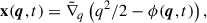
In Lagrangian formalism, we track the motion of particles x(q, t) in terms of their displacement Ψ(q, t) from initial positions q,
 (4)
(4)
In Lagrangian q-space, the density is uniform and equal to the background density in our expanding universe, that is the Eulerian x-space. The Eulerian density is given by the Jacobian of the transformation between Lagrangian and Eulerian spaces,
 (5)
(5)
 (6)
(6)
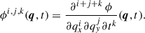
where J is the determinant of the Jacobian, and δD is the Dirac-delta function. We define the deformation matrix dij(q, t) = δijD − Jij(q, t) = − ∂Ψi / ∂qj(q, t) with eigenvalues α > β and corresponding eigenvectors  , which together encode the complete dynamical information. In terms of eigenvalues,
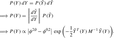
![Mathematical equation: $$ \begin{aligned} \rho (\mathbf x , t) \propto J(\boldsymbol{q},t)^{-1} = [(1 - \alpha (\boldsymbol{q},t))(1 - \beta (\boldsymbol{q},t))]^{-1}. \end{aligned} $$](/articles/aa/full_html/2026/06/aa57478-25/aa57478-25-eq10.gif) (7)
(7)
Within the framework of catastrophe theory, the particle motion can be viewed as the evolving shape of the CDM sheet in x − q space (see Fig. 1). The topology of the sheet is determined by the set of critical points: J = ∥∂xi/∂qj∥ = 0. The tangent to the sheet at critical points is perpendicular to the Eulerian space and hence, the density at these points projected onto the Eulerian space is singular, as implied by Eq. (6). From Eq. (7), the density being singular implies
 (8)
(8)
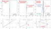 |
Fig. 1. 2D shell crossing in Eulerian x − y space (top row) along with a qx axis slice through the shell-crossing point qc in qx − x space (bottom row) to help visualize the folding of the CDM sheet. Left column: Snapshot during the single-stream flow prior to shell crossing (t < tc). Middle column: Moment of shell crossing (t = tc). A catastrophe event marked by the appearance of an A3+ singularity (red dot) seeds the 2D pancake-like structure, shown in the right column (t > tc). The boundary of the pancake encompassing the multi-streaming region is defined by A2 singularities (blue), which grows along the A3+ spine (green). |
for points undergoing shell crossing for the first time (see Sect. 5(a) in Doroshkevich & Shandarin 1978 and Eq. (10) in Arnold et al. 1982). This condition identifies the A2 class of singularities in 2D.
When shell crossing occurs for the first time in a local neighborhood, the sheet starts folding onto itself, turning perpendicular to the Eulerian space and forming a cusp. The first critical point (or singularity) appears, indicating a change in topology (or catastrophe). We refer to this point as the shell-crossing point (qc, tc). It is the first point to satisfy the condition α(q, t) = 1 in its local neighborhood and is therefore a local maximum of the eigenvalue field, that is ∇qα(q, t) = 0. In 2D, it is a singularity of class A3+, also called cusp singularity. shell crossing typically happens along one axis; it is nearly impossible to have shell crossings along multiple axes simultaneously (see Eq. (12) in Doroshkevich 1970). Therefore, as the CDM sheet folds further, its projection onto the Eulerian space is shaped like a pancake, bulging towards the center. In 2D, it is shaped like an eye. The cusps at either end of the fold in CDM sheet branch out in opposite directions ( ) transverse to the shell-crossing direction (
 ) and follow the locus of A3+ singularities (see Sect. 5(b) in Doroshkevich & Shandarin 1978 and Eq. (13) in Arnold et al. 1982), given by
 (9)
(9)
Thus, the A3+ locus serves as the spine along which the pancake grows, with its boundary (lateral edges of the fold in CDM sheet) being defined by the A2 locus Eq. (8). The A2 boundary divides the multi-stream and single-stream regions in Eulerian space. As more particles enter the multi-stream region, the size of the pancake (A2 boundary) grows, with the two A3+ singularities at either tips branching out farther.
In fact, the locus of A3+ singularities passes through all the critical – local maxima, minima, and saddle - points of the eigenvalue field, since  automatically satisfies Eq. (9). These are the points around which collapses occur and structures emerge. Therefore, the A3+ locus traces not only the spine of pancakes, but also the entire the skeletal network of structures in our 2D setup, akin to the cosmic web of the universe in 3D. Put differently, the study of the cosmic web can be reduced to analyzing the critical points of the eigenvalue field α(q, t) within the framework of Morse-Smale theory (Smale 1960).
Growing pancakes form only around points of local maxima with positive eigenvalue α. These points, which we refer to as shell-crossing points, are the focus of our formalism. If there is no shell crossing along the transverse direction(s), the pancake grows into a filament in 2D (wall in 3D). If there is shell crossing along the secondary transverse direction, the pancake turns into a cluster in 2D (filament in 3D). Further, in 3D, shell crossing along the tertiary transverse direction turns it into a cluster. Clusters, followed by violent relaxation in the multistream regime (Lynden-Bell 1967), lead to the formation of primordial halos.
On the other hand, saddle points with positive eigenvalue α undergo shell crossing to form tube-shaped structures, whereas points of local minima correspond to no physical structures. The saddle points, however, are not the first points to undergo shell crossing in their local neighborhood, which is already deep in the multi-stream regime by the time these points turn singular. Although the same formalism, with minor tweaks discussed in the next subsection, holds true for these points asymptotically, its applicability in studying the large-scale structure around these points is limited.
Equations (3)–(6) form a complete set of equations that can be solved for a given set of initial conditions. For cosmological setups, the initial conditions are generally provided in terms of the matter power-spectrum Pδ(k) of a Gaussian random field for the overdensity δ(q), defined as  , where k is the Fourier mode and δD is the Dirac-delta function.
If there is no vorticity in Lagrangian space in our setup, then the displacement field derives from a potential ϕ
 (10)
(10)
which is related to the overdensity δ(q) in the linear regime: Δqϕ(q) = δ(q). The displacement potential ϕ(q) is therefore Gaussian distributed as well, with the power spectrum
 (11)
(11)
Eq. (6) is valid as long as the flow is single-stream and one can obtain recursive solutions using LPT. After shell crossing, the flow is multistream inside the boundary of the pancake defined by A2 singularities, and LPT breaks down. Equation (6) must be modified into
 (12)
(12)
to take into account the contribution from the overlapping folds of the CDM sheet. This is the basis of post-collapse perturbation theory (PCPT; Colombi 2014; Taruya & Colombi 2017; Rampf et al. 2021; Saga et al. 2023) in which the corrections to the force field from the overlapping folds are computed that allows the post-collapse motion to be tracked deeper into the multi-stream regime.
2.2. Normal form of the shell-crossing singularity
For our purpose of studying the structure of an emerging pancake in 2D, we derived the normal form of the first singularity that appears in a local neighborhood at shell crossing. We start by expanding the motion around the shell-crossing location and time (qc, tc) into a Taylor series up to O(q3, t),
 (13)
(13)
The first assumption made is that of ballistic approximation, that is, expansion in x up to linear order in time. Higher-order expansion in time would require computation of the force field as is done in PCPT. We shall show in a following subsection (see Eq. (29) and the subsequent discussion) that in order to be self-consistent under this assumption, the expansion in velocity must be linear order in space: dx/dt ∼ O(q). The second assumption is that the motion of particles is vorticity-free in Lagrangian space,
 (14)
(14)
which is obtained by substituting Eq. (10) in Eq. (4). Thus, the coefficients of our expansion comprise derivatives of ϕ up to fourth order in q and first order in t. This assumption is justifiable for displacement fields derived from 1- or 2-LPT motion. For more generic cases, such as N-body simulations or 3-LPT and beyond, the effect of vorticity in Lagrangian space is non-negligible, but is left for future work (see Sect. 4). We use the following notation for the derivatives of ϕ:
 (15)
(15)
In equations where the function input (q, t) has been dropped to make them concise, it is to be assumed that the function is evaluated at the shell-crossing point (qc, tc). These coefficients govern the dynamics in the vicinity of the shell-crossing point (qc, tc) and therefore determine the morphology of the pancake that forms. The first-order derivatives describe the displacement of the shell-crossing point from the origin. The second-order derivatives correspond to the curvatures of the displacement potential ϕ, i.e., the eigenvalues; their signs indicate whether the resulting structure is a halo or a filament, while their magnitudes control the growth rate of caustics along each axis. The third-order derivatives represent gradients of the eigenvalues and set the relative positions of their peaks. They introduce asymmetries, such as unequal extension along the y-axis or the emergence of a C shape. The fourth-order derivatives describe the curvatures of the eigenvalue field, determining the ellipticity of the emerging pancake and producing features such as an S shape. Based on the geometry of the CDM sheet in the neighborhood of the shell-crossing point (qc, tc), we impose constraints on the set of coefficients of our Taylor expansion Eq. (13).
-
O(q0) derivatives: ϕ0, 0, 0, ϕ0, 0, 1 These neither appear in Eq. (13) nor affect the dynamics and hence are immaterial.
-
O(q1) derivatives: ϕ1, 0, 0, ϕ0, 1, 0, ϕ1, 0, 1, ϕ0, 1, 1 Upon translating on to the shell-crossing point in Lagrangian space qc = 0 and in Eulerian space x(qc, tc) = 0, the O(q1, t0) derivatives vanish: ϕ1, 0, 0, ϕ0, 1, 0 = 0. Similarly, upon subtracting the velocity at the shell-crossing point globally from the velocity field such that dx/dt (qc, tc) = 0, the O(q1, t1) derivatives vanish as well: ϕ1, 0, 1, ϕ0, 1, 1 = 0.
-
O(q2) derivatives: ϕ2, 0, 0, ϕ1, 1, 0, ϕ0, 2, 0, ϕ2, 0, 1, ϕ1, 1, 1, ϕ0, 2, 1 With the assumption of a vorticity-free displacement field in Lagrangian space, the deformation matrix dij = δijD − Jij can be rewritten by substituting Eq. (14) in Eq. (5),
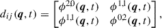 (16)
(16)which is simply the Hessian of the potential ϕ and has the eigenvalues α > β. Since dij is symmetrical, its eigenvectors
 are orthogonal (see Eqs. (A.1) and (A.2) for the full expressions of the eigenvalues and eigenvectors). By performing rotation, both in Lagrangian and Eulerian spaces, to align the reference axis
  along the shell-crossing axis
  , we diagonalize dij(qc, tc), which implies ϕ1, 1, 0 = 0 and ϕ2, 0, 0 > ϕ0, 2, 0. The eigenvalues and eigenvectors evaluated at (qc, tc) are
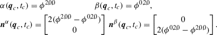 (17)
(17)The density ρ(xc, tc)∝[(1 − α(qc, tc))(1 − β(qc, tc))]−1, Eq. (7). The shell-crossing point corresponds to a singularity in the density field, which implies α(qc, tc) = ϕ2, 0, 0 = 1. If we assume Zeldovich flow prior to shell crossing, then ϕ(q, t) = D+(t)ϕ(q) implies ϕi, j, 1 ∝ ϕi, j, 0. This suggests that the constraints on the signs of ϕi, j, 1 are the same as that of ϕi, j, 0, which are ϕ2, 0, 1 > 0, ϕ1, 1, 1 = 0, ϕ2, 0, 1 > ϕ0, 2, 1. Even for higher-order LPT motion, the constraints on the signs should remain the same, as the magnitude of the corrections would typically be less than that of the leading order. Therefore, the constraints on the signs of ϕi, j, 1 are not just limited to Zeldovich flow.
-
O(q3) derivatives: ϕ3, 0, 0, ϕ2, 1, 0, ϕ1, 2, 0, ϕ0, 3, 0 The expression for
 is provided in the appendix, Eq. (A.3). Evaluating it at (qc, tc) using the previously obtained constraints ϕ1, 1, 0 = 0, ϕ2, 0, 0 = 1, ϕ2, 0, 0 > ϕ0, 2, 0 (see Eq. (109) in Feldbrugge et al. 2023),
 (18)
(18)Since the shell-crossing point is a local maximum of the eigenvalue α(q, t),
 must vanish, which implies ϕ3, 0, 0 = ϕ2, 1, 0 = 0. The other two derivatives ϕ1, 2, 0, ϕ0, 3, 0 are unconstrained. Since we restrict dx/dt up to O(q) (see Eq. (29) and the subsequent discussion), the O(q≥3, t1) derivatives of ϕ are not considered.
 -
O(q4) derivatives: ϕ4, 0, 0, ϕ3, 1, 0, ϕ2, 2, 0, ϕ1, 3, 0, ϕ0, 4, 0 The expression for the Hessian of the higher eigenvalue field, defined as Hij(α(q, t)) = ∂2α(q, t)/∂qi∂qj, is provided in the appendix, Eq. (A.4). Evaluating it at (qc, tc) using the previously obtained constraints: ϕ1, 1, 0 = 0, ϕ2, 0, 0 = 1, ϕ2, 0, 0 > ϕ0, 2, 0, ϕ3, 0, 0 = ϕ2, 1, 0 = 0 (see Eq. (6.5) in Feldbrugge & van de Weygaert 2023),
 (19)
(19)It is symmetric but not diagonal, unless ϕ3, 1, 0 = 0. Consequently, its eigenvectors
 and
and  are orthogonal, though not necessarily aligned with the eigenvectors of dij(qc, tc), namely
  and
and  , which serve as our reference axes. The expressions for the eigenvalues αH > βH and corresponding eigenvectors at (qc, tc) are provided in the appendix, Eqs. (A.5) and (A.6). For the shell-crossing point to be a non-degenerate local maximum of α(q, t), both the eigenvalues of its Hessian, which are also the curvatures at that point, must be negative. This is possible only if the trace and the determinant of the Hessian are negative and positive,
 (20)
(20)which together imply that ϕ4, 0, 0 < 0 and ϕ2, 2, 0 < 0. The remaining derivatives ϕ3, 1, 0, ϕ1, 3, 0, ϕ0, 4, 0 are unconstrained. Furthermore, the shell-crossing point (qc, tc) automatically satisfies the condition for an A3+ singularity:
 , as well as that for a ridge point:
  , by virtue of being a local maximum of α(q, tc) (see Fig. 6). The tangent to the locus of A3+ points at (qc, tc) is
  , Eq. (30), which is aligned along neither the reference axis
  nor the ridge
  in Lagrangian space unless ϕ3, 1, 0 = 0. However, it is aligned with the reference axis in Eulerian space. This is because
  gives the direction of shell crossing of particles, or the folding of the CDM sheet, which is quasi-1D for an infinitesimally small neighborhood and time interval. Therefore, the only portion of the CDM sheet in the immediate neighborhood that can continue folding lies along the transverse direction, which is
  . It is thus more straightforward to characterize the Eulerian shape of the shell-crossing structure in the frame of
  , and therein lies the reason behind our choice of the reference axes.
The final coefficient matrices ϕi, j, k after compiling all the constraints we discussed are
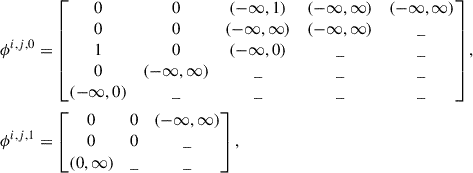 (21)
(21)
where the dashes correspond to the higher order derivatives we do not consider in our expansion.
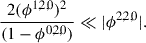
To reiterate, these constraints are derived for shell-crossing points where pancakes emerge, that is, the local maxima of the eigenvalue field α(q, t). The pancakes can be further classified into halos and filaments based on the sign of the lower eigenvalue β(qc, tc) = ϕ0, 2, 0. If ϕ0, 2, 0 ∈ (0, 1) and ϕ0, 2, 1 ∈ (0, ∞), shell crossing occurs along the transverse axis  , and the pancake collapses into a 2D halo. Conversely, if ϕ0, 2, 0, ϕ0, 2, 1 ∈ ( − ∞, 0], the particles continue to drift apart along the transverse axis without undergoing a second shell crossing, resulting in a 2D filament.
Extension to local minima and saddle points of the eigenvalue field α(q, t) is obtained simply by changing the sign constraints on the eigenvalues αH > βH of the Hessian Hij(α(qc, tc)). For saddle points, αH(qc, tc) > 0 and βH(qc, tc) < 0, which is possible only when the determinant of the Hessian is negative. If ϕ0, 2, 0 > 0, the saddle point undergoes shell crossing along the transverse axis by merging into a halo. If ϕ0, 2, 0 ≤ 0, the saddle point does not undergo further shell crossing and becomes part of a filament. For local minima, αH(qc, tc), βH(qc, tc) > 0, which is possible only when both the trace and the determinant of the Hessian are positive.
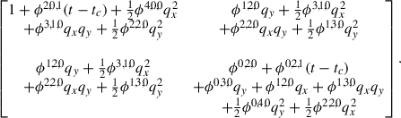
After plugging in the constraints, Eq. (21), into our expansion Eq. (13), we obtain the following reduced expression with a total of ten remaining coefficients:
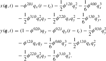 (22)
(22)
In terms of catastrophe theory, these are the normal form derivatives corresponding to the subset of A3+ singularities that appear at the local maxima of the eigenvalue α(q, t).
2.3. Pancake structure
Eq. (22) governs the motion of particles in the neighborhood of the shell-crossing location qc = 0 and time tc, from which we can derive the loci of A3+ and A2 singularities that define the structure of the emerging pancake as shown in Fig. 1.
The deformation matrix dij = δijD − Jij can be rewritten substituting our expansion form, Eq. (22), into Eq. (5). Its elements, up to O(q2, t), are
 (23)
(23)
Its eigenvalues α > β and corresponding eigenvectors  are expanded up to O(q2, t) to be consistent,
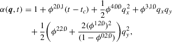 (24)
(24)
 (25)
(25)
The higher the value of 1 − ϕ0, 2, 0, the faster the convergence of these expansions. Thus, our formalism works better for collapse scenarios that have a greater difference between the eigenvalues, and hence, are closer to being quasi-1D. Substituting Eq. (24) in Eq. (8), we obtain the expression for the locus of A2 singularities at a given instant t > tc up to O(q2, t) (see Eq. (17) in Arnold et al. 1982):
 (26)
(26)
which is of the form Aqx2 + Bqxqy + Cqy2 + F = 0. It represents an ellipse if 4AC − B2 > 0. Since F > 0 for t > tc, the ellipse is real only if A, C < 0. These conditions are equivalent to Eq. (20) for the shell-crossing point to be a local maximum of the eigenvalue field α(q, t). For A, C < 0,
 (27)
(27)
 (28)
(28)
where θA2 is the angle by which the axes of the A2 ellipse  are rotated with respect to the reference frame
  at the shell-crossing point (qc, tc). The semi-major and semi-minor axes, of lengths a and b, are oriented along the directions of less and more negative curvature of α at (qc, tc), denoted by
  and
and  , respectively, and satisfy 0 < b/a ≤ 1. Consequently, the α-ridge aligns with the semi-major axis of the A2 ellipse. For the case where ϕ3, 1, 0 = B = θA2 = 0, that is, the axes of the A2 ellipse being aligned with the reference frame, the shell-crossing direction
  coincides with the minor axis (more negative curvature) if A < C < 0. Interestingly, if C < A < 0, it coincides with the major axis (less negative curvature).
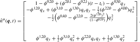
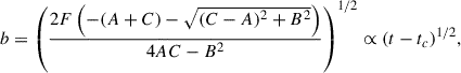
From Eq. (28), all points on the A2 ellipse satisfy |qA2 − qc|∝(t − tc)1/2. Using the parameterization h = t − tc and qA2 ∝ h1/2 in Eqs. (22) to obtain the Eulerian shape of the A2 caustic,
 (29)
(29)
The A2 caustic demarcates the multi-streaming region in Eulerian space, within which our expansion form of the motion around the shell-crossing point, Eq. (22), remains valid. Therefore, Eq. (22) is consistent up to O(h3/2). Terms of O(q2) in dx/dt would have introduced some, but not all the terms of O(h2) in xA2 leading to inconsistency. Hence, they were neglected.
For saddle points of the eigenvalue field α(q, t), the determinant of the Hessian Eq. (19) is negative, which implies 4AC − B2 < 0. Equation (26) then represents a hyperbola. For points of minima, the determinant is positive ⟹4AC − B2 > 0. However, the trace A + C being positive implies A, C > 0 for which Eq. (26) does not have real solutions after shell crossing t > tc.
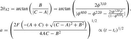
Returning to our shell-crossing point, we substitute Eqs. (24) and (25) in Eq. (9) and keep only the terms up to O(q, t) to obtain (see Eq. (5.12) in Feldbrugge & van de Weygaert 2023),
 (30)
(30)
This is the locus of A3+ points in Lagrangian space, regardless of the time when they turn singular. It is a straight line at an angle θA3 with respect to the reference axis 
 (31)
(31)
and is time-independent for our expansion form, Eq. (22), of the order O(q3, t). Higher order expansions would indeed introduce O(q≥2, t≥1) corrections (see Fig. 6 to discern the alignments between A2 ellipse, A3+ line, and the reference axes).
To obtain the Eulerian shape of the A3+ line, we substitute Eq. (30) in our expansion form Eq. (22). The expressions for xA3(q, t) and yA3(q, t) in parametric form are provided in the appendix, Eq. (A.7). It is to be noted that Eq. (30) is of O(q) and Eq. (22) is of O(q3). So, upon substitution, Eq. (A.7) for the A3+ spine is strictly correct only up to O(q). To have the complete expression of Eq. (A.7) correct up to O(q3), we need to start with expansion form, Eq. (22), of the order O(q5) that will result in Eq. (30) of the order O(q3), that is, quadratic and cubic corrections to the A3+ line in Lagrangian space. An O(q5) expansion in space necessitates O(t2) in time so that our expansion form is consistent up to O(h5/2) (see Eq. (29)). However, O(t2) expansion requires PCPT for force field corrections, which is beyond the scope of this work. Nevertheless, only at shell crossing (t = tc), the O(q) term in expansion of x(q, t), Eq. (22), vanishes and hence, the A3+ spine trajectory in Eulerian space,
![Mathematical equation: $$ \begin{aligned} x_{A3}(y_{A3}, t_c) =&- \left[ \frac{\phi ^{1,2,0}}{ 2 \left( 1 - \phi ^{0,2,0} \right)^2} \right] \, y_{A3}^2 \\&- \Bigg [ \frac{\phi ^{1,3,0} + \phi ^{3,1,0} \left( 2\left(\frac{\phi ^{3,1,0}}{\phi ^{4,0,0}}\right)^2 - 3\frac{\phi ^{2,2,0}}{\phi ^{4,0,0}} \right) }{6\left( 1 - \phi ^{0,2,0} \right)^3} \nonumber \\&+ \frac{ \phi ^{1,2,0} }{\left( 1 - \phi ^{0,2,0} \right)^4} \left(\frac{1}{2} \phi ^{0,3,0}-\frac{\phi ^{1,2,0} \phi ^{3,1,0}}{\phi ^{4,0,0}}\right) \Bigg ] \, y_{A3}^3,\nonumber \end{aligned} $$](/articles/aa/full_html/2026/06/aa57478-25/aa57478-25-eq64.gif) (32)
(32)
is indeed correct up to O(y2). The only missing term is at the order O(y3) and involves O(q5) derivative of the potential ϕ. On physical grounds, we can argue that if the field ϕ is Gaussian distributed, its O(q5) derivatives and their effects on the pancake shape are typically suppressed compared to those of the lower order derivatives for a relevant range of power spectra (see Fig. B.1 and the discussion therein). Equation (32) is therefore an accurate enough approximation at shell crossing, which is where we focus the derivation of expressions for properties related to the pancake shape.
We can transform the intersection of Eqs. (26) and (30) through Eq. (A.7) to obtain the Eulerian location of the tips of the growing pancake at instants shortly after shell crossing t > tc. From Eq. (A.7), the leading order term O(qy) in xA3(q, t) is time dependent suggesting that the spine gradually rotates. At shell crossing t = tc, however, it vanishes, which means the spine is aligned with our reference axis  . The order O(qy2) term depends on ϕ1, 2, 0 and contributes to the C shape of the spine. Last, the order O(qy3) term depends on ϕ1, 3, 0 and ϕ3, 1, 0, and contributes to the S shape of the spine.
From Eq. (32), we compute a few properties related to the shape of the pancake at shell crossing:
-
The curvature of the A3+ spine,
 (33)
(33)Doroshkevich & Shandarin (1978, in Sect. 5.3) approximated the mean curvature of the lateral surfaces (equivalent to the A2 boundary in 2D) of the pancake in 3D Eulerian space, assuming it to be infinitely thin and symmetric. It is different from the A3+ spine’s curvature Eq. (33), which is related to the leading order correction to the presumed symmetrical shape of the pancake.
-
From Eq. (32), we note that close to the shell-crossing point, the A3+ spine is C-shaped given the O(y2) term. At larger scales, it turns S-shaped as the O(y3) term starts to dominate. The transition scale provides an estimate of the extent up to which the pancake can be considered C-shaped, which we estimate using the point y at which the spine starts to bend from C to S in Eulerian space at shell crossing, that is dxA3/dyA3 (tc) = 0, which implies
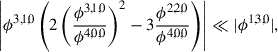
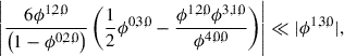
![Mathematical equation: $$ \begin{aligned} y_{C\rightarrow S}(t_c)&= -2\left( 1 - \phi ^{0,2,0} \right) \phi ^{1,2,0} \times \\&\Bigg [ \phi ^{1,3,0} + \phi ^{3,1,0} \left( 2\left(\frac{\phi ^{3,1,0}}{\phi ^{4,0,0}}\right)^2 - 3\frac{\phi ^{2,2,0}}{\phi ^{4,0,0}} \right)\nonumber \\&\quad + \frac{6 \phi ^{1,2,0}}{\left( 1 - \phi ^{0,2,0} \right)} \left(\frac{1}{2} \phi ^{0,3,0}-\frac{\phi ^{1,2,0} \phi ^{3,1,0}}{\phi ^{4,0,0}}\right) \Bigg ]^{-1}.\nonumber \end{aligned} $$](/articles/aa/full_html/2026/06/aa57478-25/aa57478-25-eq67.gif) (34)
(34)For halos, ϕ0, 2, 0, ϕ0, 2, 1 > 0, which means the transverse axis contracts. Thus, the curvature increases and the yC → S decreases with time. On the other hand, for filaments, ϕ0, 2, 0, ϕ0, 2, 1 ≤ 0, which means the transverse axis stretches, leading to decreasing curvature and increasing yC → S.
2.4. Parameters and their effects
The shape of the shell-crossing structure in Lagrangian space is captured by the loci of A2 and A3+ points, which are governed by Eqs. (26) and (30), respectively. Their transformation to Eulerian space is governed by Eq. (22). These three sets of equations constitute our analytical model and contain ten parameters in total. Constraints on the signs of some of these parameters are listed in Eq. (21). We further isolate and investigate the effect of each of these parameters on the shape of the pancake. The values of parameters used in Figs. 2, 4, 3, and 5 are only for the purpose of presentation.
-
ϕ2,0,1: velocity gradient along shell-crossing axis. It determines how quickly the particles cross trajectories and turn singular, and hence, the rate at which the A2 caustic grows in Lagrangian, Eq. (26), and Eulerian spaces.
-
ϕ2,0,0, ϕ0,2,1: displacement and velocity gradient along the transverse axis. They determine if the pancake stretches or shrinks longitudinally in Eulerian space, Eq. (22).
-
ϕ4,0,0, ϕ2,2,0: they are related to the two eigenvalues (the principal curvatures) of Hij(α(qc, tc)), Eq. (19). They determine the axis ratio of the A2 caustic, Eq. (28), which in turn affects how flat the pancake is in Eulerian space.
-
ϕ1,2,0, ϕ1,3,0: they affect the shape of the A3 spine Eq. (32) in Eulerian space. The former is responsible for the C shape, and the latter is responsible for the S shape.
-
ϕ0,3,0, ϕ0,4,0: the former adds asymmetric and the latter adds symmetric higher order corrections to the longitudinal stretch of the pancake in Eulerian space, Eq. (22).
-
ϕ3,1,0: leads to rotation of the A3+ spine at leading order and contributes to its S shape at order O(y3) in Eulerian space, Eq. (32).
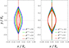 |
Fig. 2. Effect of varying ϕ2, 0, 1 (left) and ϕ0, 2, 0 (right) on the shape of A2 caustic in Eulerian space without changing the other parameters and the time. |
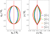 |
Fig. 3. Effect of varying the ratio ϕ2, 2, 0/ϕ4, 0, 0 on the shape of A2 caustic in Lagrangian (left) and Eulerian (right) spaces without changing the other parameters and the time. |
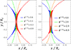 |
Fig. 4. Effect of varying ϕ1, 2, 0 (left) and ϕ1, 3, 0 (right) on the shape of A2 caustic and A3 spine in Eulerian space without changing the other parameters and the time. |
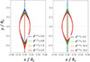 |
Fig. 5. Effect of varying ϕ0, 3, 0 (left) and ϕ0, 4, 0 (right) on the shape of A2 caustic in Eulerian space without changing the other parameters and the time. |
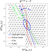 |
Fig. 6. Effect of ϕ3, 1, 0 on the shape of the A2 caustic (solid) and the A3+ spine (dashed) in Lagrangian (blue) and Eulerian (red) spaces. The angles θA2, Eq. (27), and θA3, Eq. (31), are indicated in green and blue, respectively. The vector fields of the eigenvector |

3. Gaussian statistics
Using arguments from catastrophe theory, we modeled how the derivatives of the displacement potential ϕ at the shell-crossing point (qc, tc) relate to the shape of the emerging pancake. There are ten such derivatives, or, as we prefer to call them, the parameters in our model that appear in our expansion form, Eq. (22). In this section, starting from a Gaussian random field for the displacement potential ϕ(q) and its derivatives, we compute the conditional and marginal probabilities of our model parameters subject to the constraints of a shell-crossing point, and obtain the distribution and expectation values of the features defining the shape of the pancakes.
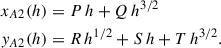
We first construct our random variables. As discussed earlier, the shape of the pancake is captured by the A2 caustic and the A3 spine. Properties like the curvature, Eq. (33), and the transition scale from C to S shape depend on O(q2),O(q3) and O(q4) derivatives of the displacement potential ϕ at shell crossing. For the purpose of computing statistics, we assume Zeldovich flow (ZA) before shell crossing. Coles et al. (1993) and Melott et al. (1994) showed that the ZA is a good approximation down to the nonlinearity scale, by which stage most pancakes have already formed yet remain relatively thin. So, ZA can be safely used to capture the time-evolution of the potential ϕ up to shell crossing: ϕ(q, t) = D+(t)ϕ(q). With this approximation, the time derivatives ϕi, j, 1s are proportional to ϕi, j, 0s, which makes their constraints redundant in the computation of conditional probabilities at the shell-crossing point. For our random variables, it is thus sufficient to consider the set of O(q2),O(q3) and O(q4) spatial derivatives for computing the properties we are interested in. The Zeldovich approximation (ZA) also allows for a rescaling of these derivatives, thereby eliminating the explicit time dependence,
 (35)
(35)
We define two random variables:  , which comprises the derivatives at a point in the generic frame, and Y, which comprises the derivatives in the reference frame (same as used in Sect. 2) rotated to align with the eigenvectors
  at that point, Eq. (A.2),
![Mathematical equation: $$ \begin{aligned}&\tilde{Y} = \left[ \tilde{\phi }^{2,0} , \tilde{\phi }^{1,1} , \tilde{\phi }^{0,2} , \tilde{\phi }^{3,0} , \tilde{\phi }^{2,1} , \tilde{\phi }^{1,2} , \tilde{\phi }^{0,3} , \tilde{\phi }^{4,0} , \tilde{\phi }^{3,1} , \tilde{\phi }^{2,2} , \tilde{\phi }^{1,3} , \tilde{\phi }^{0,4} \right],\nonumber \\&Y = \left[ \phi ^{2,0} , \theta , \phi ^{0,2} , \phi ^{3,0},\phi ^{2,1} , \phi ^{1,2} , \phi ^{0,3} , \phi ^{4,0} , \phi ^{3,1} , \phi ^{2,2} , \phi ^{1,3} , \phi ^{0,4} \right], \end{aligned} $$](/articles/aa/full_html/2026/06/aa57478-25/aa57478-25-eq72.gif) (36)
(36)
where θ is the rotation angle between the two frames, and it diagonalizes the deformation matrix:
 (37)
(37)
The transformations of the O(q3) and O(q4) derivatives under rotation, as well as the Jacobian  , are given in the appendix (Eqs. (B.1) and (B.2); see also Eqs. (E.3)–(E.5) in Feldbrugge & van de Weygaert 2023). The determinant of the Jacobian is
 (38)
(38)
We know that  is Gaussian distributed with the power spectrum
  , which is related to the matter power spectrum Pδ(k) through Eq. (11). Therefore,
  comprising derivatives of ϕ(q) is Gaussian distributed as well. Its probability density is
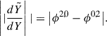
 (39)
(39)
where N is the number of elements in  and M is the covariance matrix between
  and Y, given by (see also Eqs. (57)–(65) in Feldbrugge & van de Weygaert 2025),
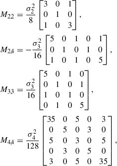 (40)
(40)
where Mi, j denotes the covariance matrix between O(qi) and O(qj) derivatives of the potential ϕ. The O(q3) derivatives have no correlation with O(q2) or O(q4) derivatives. σi refers to the ith moment of the power spectrum  ,
,
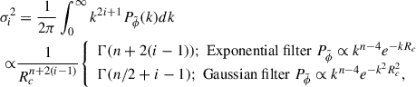 (41)
(41)
where n and Rc are the spectral index and smoothing scale, respectively. These σi encapsulate the dependence on the power spectrum parameters n, Rc as well as the smoothing filter used, thereby capturing all the statistical information about the initial potential field ϕ(q) that we require for our computations. Their dependence on the spectral index n is shown in Fig. B.1.
To obtain P(Y), we use Eqs. (39) and (38),
 (42)
(42)
The full expression after substituting  in terms of Y, Eq. (B.1), and the covariance matrix M, Eq. (40) is provided in the appendix, Eq. (B.3). This is the probability density of Y at a generic spatial point q. We are interested in the conditional probability of Y given that it is a shell-crossing point qc, that is, a peak in the eigenvalue field α(q) which seeds a pancake. For this, we take an approach similar to the computation of the number density of peaks in Bardeen et al. (1986) (see the constraints, Eq. (21)).
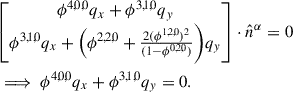
-
At shell crossing, the higher eigenvalue α(qc, tc) = ϕ2, 0, 0 is equal to 1, which implies ϕ2, 0 = D+−1(tc) > 0. For pancakes, referring to the total set of halos and filaments, it is sufficient to have α(qc, tc) > β(qc, tc)⟹ϕ2, 0 > ϕ0, 2. For the subset of halos, ϕ0, 2 must be further restricted to ϕ0, 2 > 0 to have shell crossing along the second axis as well. On the other hand, for the subset of filaments, ϕ0, 2 ≤ 0 so that the second axis does not collapse. All these constraints are introduced as Heaviside functions.
-
The shell-crossing point is a local maximum in the eigenvalue field α(q, t). This implies constraints on its gradient, ϕ3, 0, ϕ2, 1 = 0, which appear as Dirac-delta functions, and on the eigenvalues of its Hessian, Eq. (20), which appear as Heaviside functions in the conditional probability.
The conditional probability of Y can be expressed as
![Mathematical equation: $$ \begin{aligned} P \, (Y \, |&\, \mathrm{Pancake}) \propto \, P(Y) \, \delta _D(\phi ^{3,0}) \,\delta _D(\phi ^{2,1})\\&H[\phi ^{2,0}] \, H[\phi ^{2,0} - \phi ^{0,2}] \, H\left[ -\phi ^{4,0} - \phi ^{2,2} - \frac{2 (\phi ^{1,2})^2}{\phi ^{2,0} - \phi ^{0,2}} \right] \nonumber \\&H\left[ \phi ^{4,0} \left( \phi ^{2,2} + \frac{2 (\phi ^{1,2})^2}{\phi ^{2,0} - \phi ^{0,2}} \right) - (\phi ^{3,1})^2 \right],\nonumber \end{aligned} $$](/articles/aa/full_html/2026/06/aa57478-25/aa57478-25-eq87.gif) (43)
(43)
where H refers to the Heaviside function. For halo and filament populations, we need to further multiply H[ϕ0, 2] and H[−ϕ0, 2], respectively.
3.1. Marginal probabilities
The conditional probability Eq. (43) is completely parameterized by the moments of power spectrum σ2, σ3, and σ4 through Eq. (B.3). The choice of the power spectrum parameters n, Rc, and the smoothing filter affects the probability distribution only through the values of σ. If ϕi, j is uncorrelated with other derivatives, the expectation value ⟨|ϕi, j|⟩ is proportional to σi + j. Even for the correlated ones, ϕi, j / σi + j is only weakly dependent on the spectral index n (see Fig. B.2 and the discussion therein). It is thus useful to present the distributions in terms of dimensionless quantities that have been scaled by their corresponding σi + j, so that they are effectively independent of the length scale Rc, the power spectrum index n, and the smoothing filter.
From Eq. (43), we note that the marginal distribution of θ is simply constant since P(Y) Eq. (B.3) is independent of θ, and those of ϕ2, 1 and ϕ3, 0 are Dirac-delta functions centered at zero. So, we integrate them over to obtain
![Mathematical equation: $$ \begin{aligned}&P (\phi ^{2,0},\phi ^{0,2},\phi ^{1,2}, \phi ^{0,3}, \phi ^{4,0}, \phi ^{3,1}, \phi ^{2,2},\phi ^{1,3}, \phi ^{0,4} \, | \, \mathrm{Pancake}) \propto \nonumber \\&\mathrm{Exp} \Bigg [ -10\left( \frac{\phi ^{1,2}}{\sigma _3} \right)^2 - 2\left( \frac{\phi ^{0,3}}{\sigma _3} \right)^2 - \frac{1}{2} \Big ( \sum _{\mu , \nu } f_{\mu \nu }(\sigma _2, \sigma _3, \sigma _4) \phi _{\mu } \phi _{\nu } \Big )\Bigg ]\nonumber \\&|\phi ^{2,0} - \phi ^{0,2}| \, H[\phi ^{2,0}] \, H[\phi ^{2,0} - \phi ^{0,2}]\, H\left[ -\phi ^{4,0} - \phi ^{2,2} - \frac{2 (\phi ^{1,2})^2}{\phi ^{2,0} - \phi ^{0,2}} \right] \nonumber \\&H\left[ \phi ^{4,0} \left( \phi ^{2,2} + \frac{2 (\phi ^{1,2})^2}{\phi ^{2,0} - \phi ^{0,2}} \right) - (\phi ^{3,1})^2 \right], \end{aligned} $$](/articles/aa/full_html/2026/06/aa57478-25/aa57478-25-eq88.gif) (44)
(44)
where ϕμ, ϕν ∈ {ϕ2, 0, ϕ0, 2, ϕ4, 0, ϕ3, 1, ϕ2, 2, ϕ1, 3, ϕ0, 4} and fμν(σ2, σ3, σ4) is the coefficient of the product pair ϕμ, ϕν, which can be read off Eq. (B.3). Again, H[ϕ0, 2] and H[−ϕ0, 2] have to be multiplied for halo and filament populations, respectively. We can analytically calculate the marginal distribution of ϕ0, 3, since it is uncorrelated,
 (45)
(45)
which is the same across pancake, halo, and filament populations. The expectation value of its magnitude is
 (46)
(46)
The other derivatives are correlated, and analytical expressions for their distributions are not straightforward. Instead, we use the Monte Carlo method to integrate Eq. (44) and present their marginal distributions in Figs. 7, 8, and 9. The data points from numerical integration are cubically interpolated. Distributions across pancake, halo, and filament populations are shown in blue, green, and red curves, respectively. The expectation values, also evaluated numerically, are noted in Table 1. For those with symmetrical distributions (ϕ1, 2, ϕ0, 3, ϕ3, 1, ϕ1, 3), we record the expectation value of their magnitude.
 |
Fig. 7. Marginal probability densities of ϕ2, 0 (left) and ϕ0, 2 (right) scaled by σ2. |
 |
Fig. 8. Marginal probability densities of ϕ1, 2 (left) and ϕ0, 3 (right) scaled by σ3. Equation (45) is shown as the dashed black curve for comparison. |
 |
Fig. 9. Marginal probability densities of: ϕ4, 0 (solid) and ϕ2, 2 (dashed) in the top left panel, ϕ3, 1 in the top right panel, ϕ1, 3 in the bottom left panel, and ϕ0, 4 in the bottom right panel, all scaled by σ4. The points, evaluated using Monte Carlo integration, have been cubically interpolated. |
Expectation values of the derivatives of the displacement potential, scaled with respect to their corresponding σs, computed using Monte Carlo integrals for individual pancake, halo, and filament populations.
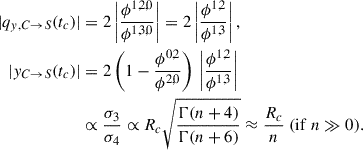
Figure 7 shows the distributions of O(q2) derivatives: ϕ2, 0/σ2 and ϕ0, 2/σ2, which correspond to the eigenvalues α(qc) and β(qc). From Eq. (7), the density,  up to leading order, depends on both the eigenvalues. On the other hand, the shell-crossing time depends only on α(qc) as D+(tc) = 1/α(qc), Eq. (47). In a Gaussian random field, the eigenvalues are correlated: points with higher α typically have higher β. Thus, the shell-crossing points, which are the peaks of α, may not correspond to the density peaks exactly, but are typically located in the overdense neighborhood. Shell-crossing points where halos appear, β > 0, have higher α and hence, are generally denser and undergo shell crossing earlier than those where filaments appear, β < 0. This is what we note from the distributions and expectation values. However unlikely, it is not entirely impossible that a point, which is less dense than another, undergoes shell crossing earlier. Also, ⟨ϕ0, 2⟩ being negative for the pancake population suggests that the fraction of filaments is higher than that of halos.
Figure 8 shows the distributions of O(q3) derivatives: ϕ1, 2/σ3 and ϕ0, 3/σ3. They are symmetrical and the same across pancake, halo, and filament populations. The numerically integrated distribution and the expectation value of ϕ0, 3/σ3 demonstrate good agreement with the analytical curve, Eq. (45), shown in black, and the expectation value, Eq. (46), respectively.
Figure 9 shows the distributions of O(q4) derivatives: ϕ4, 0, ϕ3, 1, ϕ2, 2, ϕ1, 3, and ϕ0, 4 scaled with respect to σ4. The distributions for ϕ3, 1 and ϕ1, 3 are symmetrical and show little variation across pancake, halo, and filament populations. In Eq. (B.3), ϕ3, 1 and ϕ1, 3 are correlated only with each other and have the same variance; however, the distribution for ϕ3, 1, from Eq. (44), turns out narrower, and its expectation value correspondingly lower than that of ϕ1, 3 because of the constraints on the eigenvalues of Hij(α) at the shell-crossing (local maximum) point, Eq. (20), which appear in the Heaviside function and rule out higher values of ϕ3, 1 that would instead lead to a saddle point.
The distribution of ϕ4, 0 is wider than that of ϕ2, 2, which suggests that generally A < C < 0 in Eq. (28), that is, the minor axis of the A2 ellipse is more or less aligned with the shell-crossing direction. Crudely approximated (see Eq. (54)), the semi-major and semi-minor axis lengths, a and b, are proportional to  and
and  , respectively. We may thus expect the A2 caustics to be predominantly flat. Comparing between halo and filament populations, the variation in ϕ4, 0 is less than that of ϕ2, 2. Also, the absolute means are higher for halos. This suggests that, in general, the semi-minor axis length differs little between the two populations, but the major axis length tends to be smaller for the halos than the filaments of the same age.
The marginal distributions and expectation values do have a weak dependence on the spectral index n (refer Fig. B.2); the distributions in Figs. 7–9, and the expectation values noted in Table 1 were computed assuming n = 1 and Rc = 10 grid units as representative values, along with exponential smoothing. Neglecting the weak dependence on n, ⟨|ϕi, j|⟩ ∝ σi + j ∝ Rc−n/2 − (i + j − 1). It can thus be inferred that higher n and Rc correspond to smoother density and potential fields having narrower distributions of ϕi, j.
3.2. A typical pancake
We make use of our statistical computations of the expectation values of ϕi, j (Table 1) in our analytical model of the pancake structure (Sect. 2) to demonstrate a typical pancake in a cosmology of our choice: n = 1, Rc = 10 grid units with exponential smoothing. As a note, the qualitative features of the geometrical shape of the pancake, with length scale roughly set by the peak of the matter power spectrum (≈Rc/n for n > 0), remain nearly the same regardless of our choice of cosmology and smoothing filter (see Eqs. (48) and (51)). Figure 10 shows the A2 caustic and A3 spine of this pancake at different times after shell crossing in both Lagrangian and Eulerian spaces. They are computed using Eqs. (26), (30), and (22).
 |
Fig. 10. A2 caustic (solid lines) and the A3 spine (dashed lines) of the average pancake at D+(t)−D+(tc)∈{0.001, 0.05, 0.1, 0.15} in Lagrangian (left) and Eulerian (right) space. The x-axis in Eulerian space is zoomed by 200% for clarity. |
Since ⟨ϕ0, 2⟩< 0, this pancake evolves into a filament. Looking at the A3+ spine in Eulerian space (see Eq. (32)), it is C-shaped close to the center. Its curvature turns out to be 0.036 (grid unit)−1 at (qc, tc). As expected from Eq. (33), for filaments, the curvature decreases with time, which can be observed as the A3+ spine stretching outwards from the shell-crossing point.
At larger scales, the pancake transitions to S shape. The distance from the center at which the A3+ spine bends from C to S turns out to be yC → S ≈ 4.0 grid units at shell crossing (see Eq. (34)). It increases with time as expected of filaments. Our choice of power spectrum peaks for structures of the size ≈Rc/n = 10 grid units, which is comparable to the extent of the C shape of a typical pancake ≈2yC → S. We can thus expect that the pancakes appearing in 2D cosmologies seeded by Gaussian random fields are dominantly C-shaped. In Lagrangian space, the length ratio of semi-minor to semi-major axis of the A2 caustic b/a is approximately 0.48, which changes little with time. Consequently, the Eulerian shape of the pancake turns out quite flat.
In the following subsections, we present in greater detail the distributions of the following properties:
-
Shell-crossing time D+(tc)
-
Curvature of A3+ spine d2xA3/dyA32|qc, tc
-
Length scale at which A3+ spine transitions from C to S shape 2 yC → S(tc)
-
Axis-length ratio of the A2 caustic in Lagrangian space b/a
Additionally, the differences in distributions between halo and filament populations, and the dependence of expectation values on the power spectrum parameters characterizing the 2D Gaussian random field ϕ(q) are discussed.
3.3. Distribution of shell-crossing times
The shell-crossing time can be obtained from Eq. (8) assuming Zeldovich flow,
 (47)
(47)
This suggests that a higher spectral index n and a larger smoothing scale Rc will push the initial shell crossings to later times. We obtain the marginal distribution P(ϕ2, 0 | Pancake) using Monte Carlo integration, see Fig. 7, and transform it according to Eq. (47) to obtain P(D+(tc) | Pancake). Figure 11 shows the distribution of shell-crossing times for pancake, halo, and filament populations. Their expectation values are provided in Table 2.
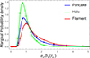 |
Fig. 11. Distribution of shell-crossing times D+(tc for pancakes (blue), halos (green), and filaments (red)). |
Expectation values of the shell-crossing time, curvature, and C-S transition of the A3+ spine and the axis-length ratio of the A2 caustic in units provided in brackets, computed using Monte Carlo integrals for the individual pancake, halo, and filament populations.
Halos undergo first shell crossing earlier than filaments on average. For our choice of cosmology n = 1 and Rc = 10 grid units with exponential smoothing, the average shell-crossing redshifts turn out to be z ≈ 1.2, 2.3, 0.8 for pancakes, halos, and filaments, respectively.
3.4. Distribution of the curvature of the A3+ spine
The curvature of the A3+ spine at shell crossing (qc, tc), Eq. (33), can be rewritten as
 (48)
(48)
This suggests that a lower spectral index n or a larger smoothing scale Rc will result in pancakes with lower curvature. We obtain the joint distribution P(ϕ2, 0, ϕ0, 2, ϕ1, 2 | Pancake) using Monte Carlo integration of Eq. (44) and transform it according to Eq. (48). Figure 12 shows the distribution of curvature for pancake, halo, and filament populations. Their expectation values are provided in Table 2.
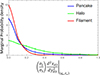 |
Fig. 12. Distribution of the curvature of the A3+ spine for pancakes (blue), halos (green), and filaments (red). |
Even though the distribution of P(ϕ1, 2) is nearly the same across pancake, halo, and filament populations, Fig. 8, halos have higher curvature than filaments. This is because they have β(qc, tc) = ϕ0, 2, 0 > 0, which indicates that the A3+ spine contracts along the y-axis, contrary to what happens in the case of filaments, refer to Eq. (33).
For our choice of cosmology n = 1 and Rc = 10 grid units with exponential smoothing, the average curvatures turn out to be ≈0.067, 0.127, 0.023 (grid unit)−1 for pancakes, halos, and filaments, respectively. The maximum possible curvature of a pancake of size corresponding to the power spectrum peak is ≈4n/Rc = 0.4 (grid unit)−1. Compared to this, the spines of pancakes at shell crossing, in particular the filaments, are mostly straight, but with noticeable bends.
3.5. Distribution of the length scale at which the A3+ spine transitions from C to S shape
The length scale at which the A3+ spine transitions from C to S shape is about 2 yC → S given by Eq. (34). However, computing the distribution P(yC → S) from it is tedious. We make a few crude approximations,
 (49)
(49)
 (50)
(50)
which reduce Eq. (34) to
 (51)
(51)
This suggests that a lower spectral index n or a larger smoothing scale Rc will result in pancakes with a greater extent of C shape. We obtain the joint distribution P(ϕ2, 0, ϕ0, 2, ϕ1, 2, ϕ1, 3 | Pancake) using Monte Carlo integration of Eq. (44) and transform it according to Eq. (51) to obtain P(yC → S(tc) | Pancake). Figure 13 shows the distribution of yC → S(tc) for pancake, halo, and filament populations. The expectation values using the exact and approximate formulae, Eqs. (34) and (51), are provided in the Table 2. Our approximation somewhat overpredicts the extent of C shape. We further cross-check our approximate P(yC → S(tc)) against the distribution measured from simulations (see Fig. C.4).
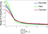 |
Fig. 13. Distribution of yC → S(tc) (solid lines) for pancakes (blue), halos (green), and filaments (red). For comparison, the distributions of qy, C → S(tc) are shown as dashed lines. |
The extent of the C shape of the A3+ spine is inversely related to that of curvature. This is because the distribution of qy, C → S(tc) is the same across pancakes, halos, and filaments, and the difference in distributions of yC → S(tc) comes from the sign of the lower eigenvalue β(qc) = ϕ0, 2 (see Eq. (51)). If a halo and a filament start off with the same qy, C → S(tc), the contraction of the A3+ spine for the halo due to its positive β(qc) results in lower yC → S(tc), whereas the opposite holds for the filament. Filaments, therefore, have A3+ spines that appear C-shaped up to larger scales than halos.
For our choice of cosmology n = 1 and Rc = 10 grid units with exponential smoothing, the average values of yC → S(tc) based on the exact Eq. (34) turn out to be ≈6.82, 3.66, 8.90 grid units for pancakes, halos, and filaments, respectively. The extent of the C shape ≈2yC → S is comparable to the scale of structures where the power spectrum peaks Rc/n ≈ 10 grid units. Thus, the pancakes, in particular the filaments, are mostly C-shaped.
3.6. Distribution of the axis-length ratio of the A2 caustic
The axis-length ratio b/a of the A2 ellipse in Lagrangian space can be computed from Eq. (28). We also made a few assumptions here,
 (52)
(52)
 (53)
(53)
The axis-length ratio reduces to
 (54)
(54)
which is time independent and scale free. We obtain the joint distribution P(ϕ4, 0, ϕ2, 2 | Pancake) using Monte Carlo integration of Eq. (44) and transform it according to Eq. (54) to obtain P( b/a | Pancake). Figure 14 shows the distribution of axis-length ratio for pancake, halo, and filament populations. Their expectation values using exact and approximate formulae, Eqs. (28) and (54), are provided in Table 2. Our approximation somewhat overpredicts the axis ratio of A2 caustics in Lagrangian space. We further cross-check our approximate P(b/a) against the distribution measured from simulations (see Fig. C.4).
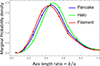 |
Fig. 14. Distribution of the axis-length ratio of the A3+ spine for pancakes (blue), halos (green), and filaments (red). |
Since ϕ is Gaussian distributed, the O(q2) and O(q4) are so correlated that the ordering of eigenvalues (by rotation) α = ϕ2, 0 ≥ β = ϕ0, 2 at the local maxima of eigenvalue α generally leads to the ordering of curvatures ϕ4, 0 ≤ ϕ2, 2 < 0, which means that the shell-crossing direction has the higher magnitude of curvature and is more or less aligned with the minor axis of the A2 ellipse in Lagrangian space. Therefore, for these cases in general, the axis ratio 0 < b/a ≤ 1 can be seen as a proxy for axis symmetry in the shell-crossing dynamics. The lower the axis ratio, the greater the difference in eigenvalues α, β, the more quasi-1D (or anisotropic) the shell crossing, the more eccentric the A2 caustic, and the flatter the pancake in Eulerian space. Axis-symmetric collapse corresponding to b/a = 1 is nearly impossible because the probability of the two eigenvalues α, β being equal is zero (see Eq. (44)). From Fig. 14, we observe that halos tend to have slightly more axis-symmetric A2 caustics than filaments. The average axis ratios, based on the exact Eq. (28) and nearly independent of cosmology and time evolution, are ≈0.469, 0.493, 0.445 for pancakes, halos, and filaments, respectively, which are still fairly anisotropic.
The analytical and statistical models we have thus presented allow us to describe the shape of the pancake given the derivatives of the displacement potential ϕ at the shell-crossing point (qc, tc), together with the probability distribution of those derivatives and several properties of pancakes that arise in Gaussian random realizations, given the power spectrum parameters n, Rc. To verify these results, we carry out simulations of Zeldovich flow initialized with Gaussian random fields, make measurements of the shape of the shell-crossing structure and the distribution of derivatives of ϕ at shell-crossing points, and compare them to our models. The details of this analysis are presented in Appendix C.
4. Conclusions
With the broader goal of understanding the cosmic web of the Universe, we studied the structure of pancakes that emerge out of the first shell crossings and their distribution in 2D cosmologies seeded by Gaussian random fields. Based on arguments from catastrophe theory, we developed an analytical model for capturing the motion and emerging structure around the point of singularity that forms at the shell crossing in 2D. We also studied the distribution of a number of observable properties of the pancakes related to their formation and shape by modeling the distribution of parameters characterizing them using Gaussian statistics. To verify our models, we performed 1-LPT simulations and compared the predicted pancake shapes and the parameter distributions with those measured in the simulations. The main results and inferences from our work are listed below.
-
The 2D cosmic web can indeed be traced using the locus of A3+ singularities, and the shape of this locus can be pieced together by studying the critical points that lie on it (Hidding et al. 2014; Feldbrugge et al. 2018). In particular, we focused on the points of local maxima because at these points, the pancakes emerge from first shell crossings and later evolve into halos and filaments. These are the key structures defining the overall cosmic web. The models for the analytical shape and statistical distribution developed for pancakes can be further extended to the saddle points on the A3+ spine through simple changes of the constraints on the model parameters (see Sect. 2.2).
-
We have presented a parameterized expansion form, correct up to O(q3, t1), for the motion around a shell-crossing point in Eq. (22) and studied the structure of the emerging pancake by tracing the A3+ spine and A2 caustic in Lagrangian and Eulerian spaces (see Eqs. (26), (30), and (22)). The effect of each parameter on the shape of the pancake was mapped out in Sect. 2.4. The most notable effects are the leading O(y2) and next-to-leading O(y3) order terms in Eq. (32), which cause the C and S shape of the pancake, respectively.
-
We have also derived an analytical expression Eq. (44) for the joint probability distribution of the parameters for the pancake, halo, and filament populations that appear in 2D cosmologies seeded by Gaussian random fields with a power spectrum characterized by the index n and smoothing scale Rc.
-
Combining Gaussian statistics with our analytical model for the pancake structure and formation, we obtained the distributions of several observable features of the pancakes, that is, shell-crossing times (Fig. 11), curvature (Fig. 12), shape transition scale (Fig. 13), and axis ratio (Fig. 14). We also noted in Table 2 the variation in their expectation values in the halo and filament populations and their scaling with power spectrum parameters n and Rc. The points on the A3+ spine that evolve into halos undergo first shell crossing earlier on average than those that evolve into filaments. The A3+ spine typically has a higher curvature at halo points than at filaments. Moreover, for halos, this curvature increases with time, whereas for filaments, it decreases. In general, the pancakes are dominantly C-shaped, and this holds more for filaments than halos. The average axis ratio of the A2 caustic of the pancakes is significantly anisotropic, which is again more so for filaments than halos.
In realistic cosmological setups, there are small-scale perturbations at all scales. We deliberately filtered small-scale perturbations in the initial conditions by introducing a smoothing scale Rc in the power spectrum. This allowed us to isolate and study the universal local structure of the earliest shell-crossing events at and above the scale Rc, under the assumption that the dynamics at scales smaller than Rc do not qualitatively distort the larger-scale pancake morphology. Our results are thus to be understood as describing the universal local structure of shell crossing under controlled smoothing. In realistic cosmological scenarios, Rc may be identified with either the nonlinearity scale RNL ∼ 5 − 10 h−1 Mpc, in which case ZA is a good approximation and our results describe coarse-grained large-scale pancakes with smaller structures that would already have undergone shell crossing essentially filtered out, or with a physical free-streaming scale RFS ∼ 1 − 10 pc for a 100 GeV CDM particle, in which case they apply to the earliest pancakes and associated small-scale filaments and microhalos, but only locally in space and time around individual shell-crossing events.
This work can be improved by including vorticity in Lagrangian space and using expansion forms of orders higher than O(q3, t1). The inclusion of vorticity will lead to a gradual rotation of the A2 ellipse and the A3+ spine in Lagrangian space and to a next-to-leading order O(q3) correction to the Eulerian shape of the pancake (Eq. (32)). On the other hand, O(q> 3) terms will introduce higher-order corrections to the shape of A3+ spine in Lagrangian space, which is only a straight line up to O(q3), Eq. (30). They will also introduce asymmetry in the width of the A2 caustic along the shell-crossing axis on either side of the central point qc. An extension to 3D is conceptually similar, but analytically cumbersome, as the number of coefficients, constraints, and parameters will increase. More importantly, it will allow us to test our predictions against observations of the large-scale structure. Systematic deviations from the predicted statistics beyond those generated by gravitational dynamics would then point to primordial non-Gaussianity in the initial conditions at the scale of shell crossing (or smoothing).
We thus demonstrated that catastrophe theory provides a natural and robust framework for describing the local pancake (shell crossing) structure in the cosmic web. Combined with Gaussian statistics, it yields statistical predictions for pancake morphologies. While these results are not yet quantitatively applicable to fully realistic multiscale nonlinear evolution, they provide a well-defined baseline against which the effects of higher-order dynamics and small-scale perturbations may be assessed.
Acknowledgments
This work is supported in part by the French Doctoral school ED127, Astronomy and Astrophysics Ile de France (AP), the Programme National Cosmology et Galaxies (PNCG) of CNRS/INSU with INP and IN2P3, co-funded by CEA and CNES, the ≪ action thématique ≫ Cosmology-Galaxies (ATCG) of the CNRS/INSU PN Astro (SC & AP), Grant ISHIZUE 2025 of Kyoto University (AT), the Japan Society for the Promotion of Science (JSPS) Overseas Research Fellowships and Invitational Fellowships for Research in Japan, the JSPS KAKENHI Grant No. 23K19050 and No. 24K17043 (SS); JP23K20844 and JP23K25868 (AT), and by the “PHC Sakura” program (project number: 51203TL, grant number: JPJSBP120243208), implemented by the French Ministry for Europe and Foreign Affairs, the French Ministry of Higher Education and Research, and the Japan Society for Promotion of Science (JSPS).
References
- Abel, T., Hahn, O., & Kaehler, R. 2012, MNRAS, 427, 61 [Google Scholar]
- Arnold, V. I. 1982, in Trudy Seminara imeni I. G. Petrovskogo, 8, 21 [Google Scholar]
- Arnold, V. I. 1983, Usp. Mat. Nauk (Russian Mathematical Surveys), 38, 77 [Google Scholar]
- Arnold, V. I. 1984, Catastrophe Theory, 1st edn. (Berlin& New York: Springer-Verlag), ix + 79 [Google Scholar]
- Arnold, V. I., Shandarin, S. F., & Zel’dovich, Y. B. 1982, Geophys. Astrophys. Fluid Dyn., 20, 111 [Google Scholar]
- Bardeen, J. M., Bond, J. R., Kaiser, N., & Szalay, A. S. 1986, ApJ, 304, 15 [Google Scholar]
- Bernardeau, F., Colombi, S., Gaztañaga, E., & Scoccimarro, R. 2002, Phys. Rep., 367, 1 [Google Scholar]
- Bond, J. R., Kofman, L., & Pogosyan, D. 1996, Nature, 380, 603 [NASA ADS] [CrossRef] [Google Scholar]
- Cautun, M., van de Weygaert, R., Jones, B. J. T., & Frenk, C. S. 2014, MNRAS, 441, 2923 [Google Scholar]
- Codis, S., Pichon, C., Devriendt, J., et al. 2012, MNRAS, 427, 3320 [NASA ADS] [CrossRef] [Google Scholar]
- Coles, P., Melott, A. L., & Shandarin, S. F. 1993, MNRAS, 260, 765 [NASA ADS] [Google Scholar]
- Colless, M., Peterson, B. A., Jackson, C., et al. 2003, arXiv e-prints [arXiv:astro-ph/0306581] [Google Scholar]
- Colombi, S. 2014, MNRAS, 446, 2902 [Google Scholar]
- de Lapparent, V., Geller, M. J., & Huchra, J. P. 1986, ApJ, 302, L1 [Google Scholar]
- DESI Collaboration (Aghamousa, A., et al.) 2016, arXiv e-prints [arXiv:1611.00036] [Google Scholar]
- Doroshkevich, A. G. 1970, Astrofizika, 6, 581 [Google Scholar]
- Doroshkevich, A. G., & Shandarin, S. F. 1978, Soviet Astron., 22, 653 [Google Scholar]
- Euclid Collaboration (Mellier, Y., et al.) 2025, A&A, 697, A1 [Google Scholar]
- Feldbrugge, J., & van de Weygaert, R. 2023, JCAP, 2023, 058 [Google Scholar]
- Feldbrugge, J., & van de Weygaert, R. 2025, MNRAS, 539, 873 [Google Scholar]
- Feldbrugge, J., de Weygaert, R. v., Hidding, J., & Feldbrugge, J. 2018, JCAP, 2018, 027 [CrossRef] [Google Scholar]
- Feldbrugge, J., Yan, Y., & van de Weygaert, R. 2023, MNRAS, 526, 5031 [Google Scholar]
- Gott, J. R., III, Jurić, M., Schlegel, D., et al. 2005, ApJ, 624, 463 [NASA ADS] [CrossRef] [Google Scholar]
- Gurbatov, S. N., Saichev, A. I., & Shandarin, S. F. 1989, MNRAS, 236, 385 [Google Scholar]
- Hidding, J., Shandarin, S., & van de Weygaert, R. 2014, MNRAS, 437, 3442 [Google Scholar]
- Huchra, J. P., Macri, L. M., Masters, K. L., et al. 2012, ApJS, 199, 26 [Google Scholar]
- Jõeveer, M., Einasto, J., & Tago, E. 1978, MNRAS, 185, 357 [Google Scholar]
- Kitaura, F.-S., Ata, M., Rodriguez-Torres, S., et al. 2019, MNRAS, 485, 213 [Google Scholar]
- Libeskind, N. I., van de Weygaert, R., & Cautun, M. 2018, MNRAS, 473, 1195 [Google Scholar]
- Lynden-Bell, D. 1967, MNRAS, 136, 101 [Google Scholar]
- Melott, A. L., Pellman, T. F., & Shandarin, S. F. 1994, MNRAS, 269, 626 [NASA ADS] [Google Scholar]
- Novikov, D., Colombi, S., & Doré, O. 2006, MNRAS, 366, 1201 [NASA ADS] [Google Scholar]
- Peebles, P. J. E. 1980, The Large-Scale Structure of the Universe (Princeton University Press) [Google Scholar]
- Planck Collaboration VI. 2020, A&A, 641, A6 [NASA ADS] [CrossRef] [EDP Sciences] [Google Scholar]
- Rampf, C., Frisch, U., & Hahn, O. 2021, MNRAS, 505, L90 [NASA ADS] [CrossRef] [Google Scholar]
- Saga, S., Colombi, S., & Taruya, A. 2023, A&A, 678, A168 [NASA ADS] [CrossRef] [EDP Sciences] [Google Scholar]
- Shandarin, S., Habib, S., & Heitmann, K. 2012, Phys. Rev. D, 85, 083005 [Google Scholar]
- Smale, S. 1960, Bull. Am. Math. Soc., 66, 43 [Google Scholar]
- Sousbie, T., Pichon, C., Colombi, S., Novikov, D., & Pogosyan, D. 2008, MNRAS, 383, 165 [Google Scholar]
- Springel, V., White, S. D. M., & Jenkins, A. e. a. 2005, Nature, 435, 629 [Google Scholar]
- Taruya, A., & Colombi, S. 2017, MNRAS, 470, 4858 [Google Scholar]
- Zel’dovich, Y. B. 1970, A&A, 5, 84 [NASA ADS] [Google Scholar]
Appendix A: Analytical model using catastrophe theory
The expressions for the eigenvalues α > β and eigenvectors nα, nβ of dij are
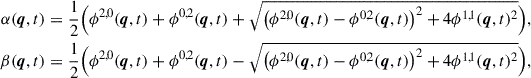 (A.1)
(A.1)
 (A.2)
(A.2)
The expressions for the components of ∇qα(q, t) are
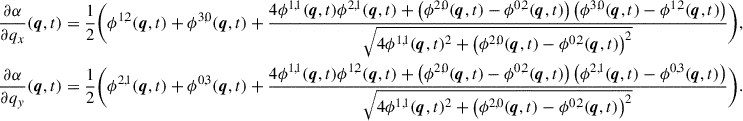 (A.3)
(A.3)
The full expression for the Hessian of the eigenvalue field α(q, t) is
![Mathematical equation: $$ \begin{aligned} \nonumber H_{11} =&\frac{1}{2} \Bigg (-\frac{\left(4 \phi ^{1,1}(\boldsymbol{q},t) \phi ^{2,1}(\boldsymbol{q},t)+\left(\phi ^{2,0}(\boldsymbol{q},t)-\phi ^{0,2}(\boldsymbol{q},t)\right) \left(\phi ^{1,2}(\boldsymbol{q},t)-\phi ^{3,0}(\boldsymbol{q},t)\right)\right)^2}{\left(4 \phi ^{1,1}(\boldsymbol{q},t)^2+\left(\phi ^{2,0}(\boldsymbol{q},t)-\phi ^{0,2}(\boldsymbol{q},t)\right)^2\right)^{3/2}} + \phi ^{2,2}(\boldsymbol{q},t) + \phi ^{4,0}(\boldsymbol{q},t) \\ \nonumber&+ \frac{4 \phi ^{2,1}(\boldsymbol{q},t)^2+\left(\phi ^{1,2}(\boldsymbol{q},t)-\phi ^{3,0}(\boldsymbol{q},t)\right)^2+4 \phi ^{1,1}(\boldsymbol{q},t) \phi ^{3,1}(\boldsymbol{q},t)+\left(\phi ^{0,2}(\boldsymbol{q},t)-\phi ^{2,0}(\boldsymbol{q},t)\right) \left(\phi ^{2,2}(\boldsymbol{q},t)-\phi ^{4,0}(\boldsymbol{q},t)\right)}{\sqrt{4 \phi ^{1,1}(\boldsymbol{q},t)^2+\left(\phi ^{2,0}(\boldsymbol{q},t)-\phi ^{0,2}(\boldsymbol{q},t)\right)^2}}\Bigg ), \\ \nonumber H_{12} =&\frac{1}{2} \Bigg [ \phi ^{1,3}(\boldsymbol{q},t) + \phi ^{3,1}(\boldsymbol{q},t) + \frac{1}{\left(4 \phi ^{1,1}(\boldsymbol{q},t)^2+\left(\phi ^{2,0}(\boldsymbol{q},t)-\phi ^{0,2}(\boldsymbol{q},t)\right)^2\right)^{3/2}} \Bigg ( \left( 4 \phi ^{1,1}(\boldsymbol{q},t)^2+\left(\phi ^{2,0}(\boldsymbol{q},t)-\phi ^{0,2}(\boldsymbol{q},t)\right)^2 \right)\\ \nonumber&\Big (4 \phi ^{1,1}(\boldsymbol{q},t) \phi ^{2,2}(\boldsymbol{q},t)+\phi ^{0,3}(\boldsymbol{q},t) \left(\phi ^{1,2}(\boldsymbol{q},t)-\phi ^{3,0}(\boldsymbol{q},t)\right)+\phi ^{2,1}(\boldsymbol{q},t) \left(3 \phi ^{1,2}(\boldsymbol{q},t)+\phi ^{3,0}(\boldsymbol{q},t)\right)\\ \nonumber&+\left(\phi ^{0,2}(\boldsymbol{q},t)-\phi ^{2,0}(\boldsymbol{q},t)\right) \left(\phi ^{1,3}(\boldsymbol{q},t)-\phi ^{3,1}(\boldsymbol{q},t)\right)\Big ) \\ \nonumber&-\left(4 \phi ^{1,1}(\boldsymbol{q},t) \phi ^{1,2}(\boldsymbol{q},t)+\left(\phi ^{0,2}(\boldsymbol{q},t)-\phi ^{2,0}(\boldsymbol{q},t)\right) \left(\phi ^{0,3}(\boldsymbol{q},t)-\phi ^{2,1}(\boldsymbol{q},t)\right)\right) \\ \nonumber&\left(4 \phi ^{1,1}(\boldsymbol{q},t) \phi ^{2,1}(\boldsymbol{q},t)+\left(\phi ^{0,2}(\boldsymbol{q},t)-\phi ^{2,0}(\boldsymbol{q},t)\right) \left(\phi ^{1,2}(\boldsymbol{q},t)-\phi ^{3,0}(\boldsymbol{q},t)\right)\right) \Bigg ) \Bigg ],\\ \nonumber H_{22} =&\frac{1}{2} \Bigg (-\frac{\left(4 \phi ^{1,1}(\boldsymbol{q},t) \phi ^{1,2}(\boldsymbol{q},t)+\left(\phi ^{0,2}(\boldsymbol{q},t)-\phi ^{2,0}(\boldsymbol{q},t)\right) \left(\phi ^{0,3}(\boldsymbol{q},t)-\phi ^{2,1}(\boldsymbol{q},t)\right)\right)^2}{\left(4 \phi ^{1,1}(\boldsymbol{q},t)^2+\left(\phi ^{2,0}(\boldsymbol{q},t)-\phi ^{0,2}(\boldsymbol{q},t)\right)^2\right)^{3/2}}-\phi ^{0,4}(\boldsymbol{q},t) -\phi ^{2,2}(\boldsymbol{q},t) \\&+\frac{\left(\phi ^{0,3}(\boldsymbol{q},t)-\phi ^{2,1}(\boldsymbol{q},t)\right)^2+4 \left(\phi ^{1,2}(\boldsymbol{q},t)^2+\phi ^{1,1}(\boldsymbol{q},t) \phi ^{1,3}(\boldsymbol{q},t)\right)+\left(\phi ^{0,2}(\boldsymbol{q},t)-\phi ^{2,0}(\boldsymbol{q},t)\right) \left(\phi ^{0,4}(\boldsymbol{q},t)-\phi ^{2,2}(\boldsymbol{q},t)\right)}{\sqrt{4 \phi ^{1,1}(\boldsymbol{q},t)^2+\left(\phi ^{2,0}(\boldsymbol{q},t)-\phi ^{0,2}(\boldsymbol{q},t)\right)^2}}\Bigg ). \end{aligned} $$](/articles/aa/full_html/2026/06/aa57478-25/aa57478-25-eq105.gif) (A.4)
(A.4)
The expressions for the eigenvalues αH > βH and eigenvectors nHα, nHβ of Hij(α) at (qc, tc) are
![Mathematical equation: $$ \begin{aligned} \alpha _H(\boldsymbol{q}_c,t_c)&= \frac{1}{2} \Bigg [ \left( \phi ^{4,0,0} + \phi ^{2,2,0} + \frac{2 (\phi ^{1,2,0})^2}{1 - \phi ^{0,2,0}} \right) + \sqrt{ \left( \phi ^{4,0,0} - \phi ^{2,2,0} - \frac{2 (\phi ^{1,2,0})^2}{1 - \phi ^{0,2,0}} \right)^2 + 4 (\phi ^{3,1,0})^2} \Bigg ],\nonumber \\ \beta _H(\boldsymbol{q}_c,t_c)&= \frac{1}{2} \Bigg [ \left( \phi ^{4,0,0} + \phi ^{2,2,0} + \frac{2 (\phi ^{1,2,0})^2}{1 - \phi ^{0,2,0}} \right) - \sqrt{ \left( \phi ^{4,0,0} - \phi ^{2,2,0} - \frac{2 (\phi ^{1,2,0})^2}{1 - \phi ^{0,2,0}} \right)^2 + 4 (\phi ^{3,1,0})^2} \Bigg ],\end{aligned} $$](/articles/aa/full_html/2026/06/aa57478-25/aa57478-25-eq106.gif) (A.5)
(A.5)
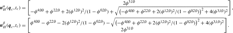 (A.6)
(A.6)
The complete equations for the shape of the A3+ spine about a shell-crossing point in Eulerian space are
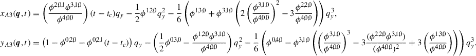 (A.7)
(A.7)
Appendix B: Gaussian statistics
The transformation of O(q3) and O(q4) derivatives of the potential ϕ under rotation by θ is given by
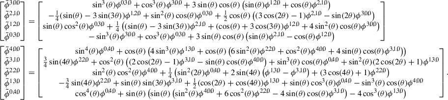 (B.1)
(B.1)
The Jacobian matrices for O(q2), O(q3), and O(q4) derivatives of ϕ, individually, are
 (B.2)
(B.2)
Their determinants are |ϕ2, 0, 0 − ϕ0, 2, 0|, 1, and 1, respectively.
The full expression for the probability density of Y:
 (B.3)
(B.3)
Our statistical results, that is, the distributions and expectation values, depend on the power spectrum parameters n, Rc solely through the σs (see Eq. (44)). Equation (41) shows that σi has a simple power-law fall-off with the smoothing scale Rc. In the left panel of Fig. B.1, we show the dependence of σs on the spectral index n, assuming exponential smoothing. The case n = −2 corresponds to the scale-invariant CDM power spectrum in 2D, while larger values of n are characteristic of warm dark matter models. Consequently, the physically relevant range of n is typically ( − 2, 5], within which we adopt n = 1 as our representative choice.
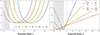 |
Fig. B.1. Variation of σi (left) and σi/σi − 1 (right) with the spectral index n (fixed smoothing scale R and exponential filter in Eq. (41)). |
The highest order term in Eq. (30) for the A3+ spine is proportional to O(q4) derivative of ϕ, which is typically of the magnitude σ4 since ⟨|ϕi, j|⟩ ∝ σi + j. Higher order expansions would introduce terms proportional to O(q5) and O(q6) derivatives of ϕ, which are of magnitudes ≈σ5/2 and σ6/6, respectively. These would successively turn significant when σ5/2σ4 ≈ 1 and σ6/3σ5 ≈ 1. In the right panel of Fig. B.1, we show how the ratio of successive moments σi/σi − 1 vary with the spectral index n assuming exponential smoothing, from which we note that the O(q5) and O(q6) derivatives of ϕ turn significant for n ⪆ 13 and n ⪆ 21, respectively. Therefore, for n ∈ ( − 2, 5], neglecting O(q5) derivatives in Eq. (32) (and in the derivations for properties like curvature and C-S transition scale) is a good enough approximation for the pancake shape.
By scaling our results with the corresponding σs, we make them scale-free, that is, independent of Rc. For uncorrelated derivatives, the distributions of ϕi, j/σi + j are also independent of n, whereas those of the correlated derivatives do show some n-dependence, as shown in Fig. B.2. The variations in the distributions of ϕ2, 0/σ2, ϕ0, 2/σ2, and ϕ4, 0/σ4 are indeed noticeable with the expectation values varying within 10% of the FWHM, which is certainly not strong enough to alter our main inferences, at least for n ∈ ( − 2, 5]. The other correlated derivatives, that is, ϕ1, 2/σ3, ϕ1, 3/σ4, ϕ3, 1/σ4, ϕ0, 4/σ4, show even less variation. We can thus expect that the distributions of derived properties, such as curvature and C-S transition scale (see Figs. 11-14), when scaled by the appropriate σs, remain largely independent of n within the physically relevant range n ∈ ( − 2, 5].
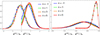 |
Fig. B.2. Marginal distributions of ϕ2, 0/σ2 (solid) and ϕ0, 2/σ2 (dashed) in the left panel, and ϕ4, 0/σ4 (solid) and ϕ2, 2/σ4 (dashed) in the right panel for different values of the spectral index n. |
Appendix C: Numerical verification
We carry out numerical simulations to verify the analytical model based on catastrophe theory for pancake shapes presented in Sect. 2, as well as the distribution of pancake shapes derived from Gaussian statistics in Sect. 3. These simulations serve as consistency checks of the relations and distributions obtained analytically; accordingly, aside from discrete sampling and finite-volume effects, the numerical measurements are expected to agree with the analytical predictions.
We initialize a grid of 5122 particles using Gaussian distributed δ(q) with the matter power spectrum of the form Pδ(k)∝knexp(−k/Rc), corresponding to parameters n = 1, Rc = 10 with exponential smoothing. The smoothing scale Rc = 10 is small (roughly 2%) compared to the grid size 512, so that the bias introduced by periodic boundaries is minimized. The particles are evolved according to Zeldovich flow, that is, the 1-LPT solution to the equations of motion (3). Since we assume no vorticity in Lagrangian space, the motion of the particles must derive from a potential, and thus, we must restrict to 1- or 2-LPT motion in our simulations. We present comparisons against Zeldovich (1-LPT) simulations since we assumed the same in our computation of Gaussian statistics.
Figure C.1 shows a snapshot from our 1-LPT simulation. To measure the A3+ and A2 singularities in our simulation, we compute the eigenvalues and eigenvectors of the deformation matrix derived from the initial displacement field in our simulations. We make a 2D interpolation of the eigenvalue α(q, t) and the dot product 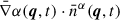 in Lagrangian space and then compute their contours in Lagrangian space according to Eq. (8) for A2 and Eq. (9) for A3+. The shell-crossing points are identified as local maxima of α(q, t). These measurements are therefore independent of the expansion form, eq (22), which forms the basis of our analytical predictions for the shape of the pancakes.
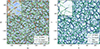 |
Fig. C.1. Snapshot from 5122 1-LPT simulation corresponding to power spectrum n = 1, Rc = 10. Left: Color-map of the higher eigenvalue α(q) in Lagrangian space. Right: Particles in Eulerian space. Points of local maxima of the eigenvalue field are highlighted in red. The A3+ spine and A2 caustics are shown as green and blue curves, respectively. |
Measurements of the A2 caustics and A3+ spines for three selected shell crossings in Eulerian space are shown in Fig. C.2. Analytical predictions for the same have been overplotted for comparison. They are computed using Eqs. (26), (30), and (22) with the values of the derivatives of ϕ at the shell-crossing point taken from the simulation. The A3+ spine shows great agreement close to the shell-crossing point and starts deviating only at the extremities. The same goes for the A2 caustic, whose extent along the x-axis agrees very well, but that along the y-axis lags behind.
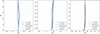 |
Fig. C.2. Three selected shell-crossing structures in a 1-LPT simulation initialized using Gaussian random field with the power-spectrum parameters n = 1, Rc = 10. The A3+ spine and A2 caustic measured from the simulation are shown in solid lines. For comparison, the A3+ spine and A2 caustic predicted from our analytical model are shown in dashed lines. |
To verify our statistical results, we perform ≈50 realizations of Gaussian random fields with the parameters n = 1, Rc = 10 and compile all the shell-crossing points (≈3500) that emerge. We record the values of derivatives of ϕ at the points of shell crossing, scale them with respect to their corresponding σ and shell-crossing time D+(tc), Eq. (35), and compare the histograms thus obtained with the marginal distributions (see Figs. 7-9) computed using Monte Carlo integrations of Eq. (44). Figure C.3 shows good agreement between the distributions from simulation measurements (shown in step histograms) and those from our semi-analytic computations (shown in interpolated curves). In particular, we notice that the simulation measurement for ϕ4, 0 falls short of the prediction for values close to 0. This could be because in our simulations, we fail to detect those peaks of α that are locally very smooth and have small heights.
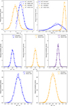 |
Fig. C.3. Comparison between marginal probability densities of derivatives of ϕ measured within the pancake population in 1-LPT simulations initialized using Gaussian random field with the parameters n = 1, Rc = 10 (shown in step histograms) and those computed using Monte Carlo integration of Eq. (44) for the same set of parameters (n, Rc) (shown in interpolated curves). |
We also make similar measurements for shell-crossing times, curvature, C-S transition scale, and axis-length ratio of the pancake population by recording the values of the combinations of ϕ derivatives given in Eqs. (47)-(54) at the points of shell crossing in our simulations. We compare these histograms to the predicted curves (from Figs. 11-14) in Fig. C.4. For C-S transition scale and axis-length ratio, we also show the histograms (orange) corresponding to the exact Eqs. (34) and (28), respectively, to cross-check our approximations in Sects. 3.5 and 3.6. In the case of the C-S transition scale, the additional terms contributing to the S shape of the pancake in the exact Eq. (34) reduce the extent of the C shape compared to the approximate Eq. (51), as expected, and hence, the exact distribution of P(yC → S(tc)) is narrower. In the case of the axis-length ratio, the exact distribution P(b/a) is shifted to lower values compared to our approximation. This indicates that the pancakes are flatter and the dynamics more anisotropic than our approximate Eq. (54) seems to suggest. Nevertheless, in both cases, save for the slight overshoot, our crude approximations exhibit surprisingly good agreement with the exact formulae, demonstrating that the additional contributions are indeed relatively small.
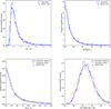 |
Fig. C.4. Comparison between marginal probability densities of shell-crossing times (top left), curvature (top right), C-S transition scale (bottom left), and axis-length ratio (bottom right) measured within the pancake population in 1-LPT simulations initialized using Gaussian random field with the parameters n = 1, Rc = 10 (shown in step histograms) and those computed using Monte Carlo integration of Eq. (44) and transformation through Eqs. (47), (48), (51), and (54) for the same set of parameters (n, Rc) (shown in interpolated curves). |
It is to be noted that the agreement shown in Fig. C.4 only verifies our semi-analytic computations of the distributions of ϕi, j combinations given in Eqs. (47)–(54), as shown in Figs. 11-14. It does not verify if those combinations, Eqs. (47)–(54), indeed map to the observable features regarding the shape of the pancake, such as the curvature and C-S transition scale. As an independent test, we could also fit x − y curves in Eulerian space to the A3+ spines of pancakes identified in our simulations, compute the curvature and yC → S from the fits, and match their distribution against the predicted curves, Figs. 12 and 13. This is left for consideration in future works. Nevertheless, given the good agreement between the shapes of the A2 caustics and A3+ spines measured in our simulations and those predicted using our analytical formalism, as shown in Fig. C.2, we expect that our statistical predictions for the pancakes’ properties, Figs. 11-14, would be in close agreement with those measured using numerical fits to the Eulerian shapes of the pancakes in simulations, a testament to the validity of Eqs. (47)–(54) in predicting observable features about the pancakes.
All Tables
Expectation values of the derivatives of the displacement potential, scaled with respect to their corresponding σs, computed using Monte Carlo integrals for individual pancake, halo, and filament populations.
Expectation values of the shell-crossing time, curvature, and C-S transition of the A3+ spine and the axis-length ratio of the A2 caustic in units provided in brackets, computed using Monte Carlo integrals for the individual pancake, halo, and filament populations.
All Figures
|
Fig. 1. 2D shell crossing in Eulerian x − y space (top row) along with a qx axis slice through the shell-crossing point qc in qx − x space (bottom row) to help visualize the folding of the CDM sheet. Left column: Snapshot during the single-stream flow prior to shell crossing (t < tc). Middle column: Moment of shell crossing (t = tc). A catastrophe event marked by the appearance of an A3+ singularity (red dot) seeds the 2D pancake-like structure, shown in the right column (t > tc). The boundary of the pancake encompassing the multi-streaming region is defined by A2 singularities (blue), which grows along the A3+ spine (green). |
| In the text | |
|
Fig. 2. Effect of varying ϕ2, 0, 1 (left) and ϕ0, 2, 0 (right) on the shape of A2 caustic in Eulerian space without changing the other parameters and the time. |
| In the text | |
|
Fig. 3. Effect of varying the ratio ϕ2, 2, 0/ϕ4, 0, 0 on the shape of A2 caustic in Lagrangian (left) and Eulerian (right) spaces without changing the other parameters and the time. |
| In the text | |
|
Fig. 4. Effect of varying ϕ1, 2, 0 (left) and ϕ1, 3, 0 (right) on the shape of A2 caustic and A3 spine in Eulerian space without changing the other parameters and the time. |
| In the text | |
|
Fig. 5. Effect of varying ϕ0, 3, 0 (left) and ϕ0, 4, 0 (right) on the shape of A2 caustic in Eulerian space without changing the other parameters and the time. |
| In the text | |
|
Fig. 6. Effect of ϕ3, 1, 0 on the shape of the A2 caustic (solid) and the A3+ spine (dashed) in Lagrangian (blue) and Eulerian (red) spaces. The angles θA2, Eq. (27), and θA3, Eq. (31), are indicated in green and blue, respectively. The vector fields of the eigenvector |
| In the text | |
|
Fig. 7. Marginal probability densities of ϕ2, 0 (left) and ϕ0, 2 (right) scaled by σ2. |
| In the text | |
|
Fig. 8. Marginal probability densities of ϕ1, 2 (left) and ϕ0, 3 (right) scaled by σ3. Equation (45) is shown as the dashed black curve for comparison. |
| In the text | |
|
Fig. 9. Marginal probability densities of: ϕ4, 0 (solid) and ϕ2, 2 (dashed) in the top left panel, ϕ3, 1 in the top right panel, ϕ1, 3 in the bottom left panel, and ϕ0, 4 in the bottom right panel, all scaled by σ4. The points, evaluated using Monte Carlo integration, have been cubically interpolated. |
| In the text | |
|
Fig. 10. A2 caustic (solid lines) and the A3 spine (dashed lines) of the average pancake at D+(t)−D+(tc)∈{0.001, 0.05, 0.1, 0.15} in Lagrangian (left) and Eulerian (right) space. The x-axis in Eulerian space is zoomed by 200% for clarity. |
| In the text | |
|
Fig. 11. Distribution of shell-crossing times D+(tc for pancakes (blue), halos (green), and filaments (red)). |
| In the text | |
|
Fig. 12. Distribution of the curvature of the A3+ spine for pancakes (blue), halos (green), and filaments (red). |
| In the text | |
|
Fig. 13. Distribution of yC → S(tc) (solid lines) for pancakes (blue), halos (green), and filaments (red). For comparison, the distributions of qy, C → S(tc) are shown as dashed lines. |
| In the text | |
|
Fig. 14. Distribution of the axis-length ratio of the A3+ spine for pancakes (blue), halos (green), and filaments (red). |
| In the text | |
|
Fig. B.1. Variation of σi (left) and σi/σi − 1 (right) with the spectral index n (fixed smoothing scale R and exponential filter in Eq. (41)). |
| In the text | |
|
Fig. B.2. Marginal distributions of ϕ2, 0/σ2 (solid) and ϕ0, 2/σ2 (dashed) in the left panel, and ϕ4, 0/σ4 (solid) and ϕ2, 2/σ4 (dashed) in the right panel for different values of the spectral index n. |
| In the text | |
|
Fig. C.1. Snapshot from 5122 1-LPT simulation corresponding to power spectrum n = 1, Rc = 10. Left: Color-map of the higher eigenvalue α(q) in Lagrangian space. Right: Particles in Eulerian space. Points of local maxima of the eigenvalue field are highlighted in red. The A3+ spine and A2 caustics are shown as green and blue curves, respectively. |
| In the text | |
|
Fig. C.2. Three selected shell-crossing structures in a 1-LPT simulation initialized using Gaussian random field with the power-spectrum parameters n = 1, Rc = 10. The A3+ spine and A2 caustic measured from the simulation are shown in solid lines. For comparison, the A3+ spine and A2 caustic predicted from our analytical model are shown in dashed lines. |
| In the text | |
|
Fig. C.3. Comparison between marginal probability densities of derivatives of ϕ measured within the pancake population in 1-LPT simulations initialized using Gaussian random field with the parameters n = 1, Rc = 10 (shown in step histograms) and those computed using Monte Carlo integration of Eq. (44) for the same set of parameters (n, Rc) (shown in interpolated curves). |
| In the text | |
|
Fig. C.4. Comparison between marginal probability densities of shell-crossing times (top left), curvature (top right), C-S transition scale (bottom left), and axis-length ratio (bottom right) measured within the pancake population in 1-LPT simulations initialized using Gaussian random field with the parameters n = 1, Rc = 10 (shown in step histograms) and those computed using Monte Carlo integration of Eq. (44) and transformation through Eqs. (47), (48), (51), and (54) for the same set of parameters (n, Rc) (shown in interpolated curves). |
| In the text | |
Current usage metrics show cumulative count of Article Views (full-text article views including HTML views, PDF and ePub downloads, according to the available data) and Abstracts Views on Vision4Press platform.
Data correspond to usage on the plateform after 2015. The current usage metrics is available 48-96 hours after online publication and is updated daily on week days.
Initial download of the metrics may take a while.