| Issue |
A&A
Volume 710, June 2026
|
|
|---|---|---|
| Article Number | A87 | |
| Number of page(s) | 16 | |
| Section | Extragalactic astronomy | |
| DOI | https://doi.org/10.1051/0004-6361/202658967 | |
| Published online | 03 June 2026 | |
DustPedia and Local Volume Legacy samples as benchmarks for dust evolution in galaxies
1
INAF – Osservatorio Astrofisico di Arcetri, Largo E. Fermi 5, 50125 Florence, Italy
2
STAR Institute, Université de Liège, Quartier Agora, Allée du six Aout 19c, B-4000 Liege, Belgium
3
Sterrenkundig Observatorium Universiteit Gent, Krijgslaan 281 S9, B-9000 Gent, Belgium
4
Université Paris-Saclay, Université Paris Cité, CEA, CNRS, AIM, 91191 Gif-sur-Yvette, France
5
INAF – Istituto di Radioastronomia, Via Gobetti 101, 40129 Bologna, Italy
6
INAF – Osservatorio di Astrofisica e Scienza dello Spazio di Bologna, via Gobetti 93/3, 40129 Bologna, Italy
7
National Observatory of Athens, Institute for Astronomy, Astrophysics, Space Applications and Remote Sensing, Ioannou Metaxa and Vasileos Pavlou, GR-15236 Athens, Greece
8
Dipartimento di Fisica e Astronomia, Alma Mater Studiorum Università di Bologna, Via Piero Gobetti 93/2, I-40129 Bologna, Italy
9
Cosmic Dawn Center (DAWN), Denmark
10
DTU-Space, Technical University of Denmark, Elektrovej 327, 2800 Kgs. Lyngby, Denmark
11
Niels Bohr Institute, University of Copenhagen, Jagtvej 128, DK-2200 Copenhagen, Denmark
★ Corresponding author: This email address is being protected from spambots. You need JavaScript enabled to view it.
Received:
14
January
2026
Accepted:
9
April
2026
Abstract
Aims. DustPedia and Local Volume Legacy (LVL) are two samples representative of the local galaxy population, including in total ∼1000 unique objects of all morphological types, with a wide range of stellar masses and star formation activity, and a spectral coverage from the ultraviolet to the far-infrared. The purpose of this work is to show that these samples cover two complementary ranges in stellar mass and galaxy morphology, making them an ideal set for constraining the dominant processes in the evolution of the galactic dust content.
Methods. Using the multi-wavelength data provided by the two surveys, we fitted the galaxies’ spectral energy distribution and estimated their physical properties, in particular the stellar mass, M*, the specific dust mass, sMdust = Mdust/M*, and the specific star formation rate, sSFR = SFR/M*.
Results. By combining DustPedia and LVL, we highlight that the trend of log10(sMdust) with log10(M*) is not monotonic. Thanks to a large number of objects across a wide range of M*, we have been able to fit two smoothly joined linear correlations: a positive one for log10(M*/M⊙)≲9.5 (a range populated mostly by LVL late spirals and irregulars), and a negative one for larger-mass, mainly DustPedia, spirals (with early-type galaxies being distinct and more dispersed in the same mass regime). For log10(M*/M⊙) > 9.5, we confirm a strong correlation between sMdust and sSFR; dwarf galaxies, instead, lie below this trend, showing a large scatter of sMdust for −10.5 < log10(sSFR/yr−1) < − 9.0. By using chemical evolution models we find that the observed log10(sMdust)–log10(M*) and log10(sMdust)–log10(sSFR) trends can be interpreted mainly by variations in the initial gas mass budget and the galaxy ages, respectively. Low-mass Sm-Irr galaxies with low sMdust and a high sSFR can only be reproduced by the models by assuming a highly efficient photofragmentation rate of large grains, and/or low grain growth in clouds.
Key words: dust / extinction / galaxies: evolution / galaxies: fundamental parameters / galaxies: general / galaxies: ISM / galaxies: star formation
© The Authors 2026
 Open Access article, published by EDP Sciences, under the terms of the Creative Commons Attribution License (https://creativecommons.org/licenses/by/4.0), which permits unrestricted use, distribution, and reproduction in any medium, provided the original work is properly cited.
This article is published in open access under the Subscribe to Open model. This email address is being protected from spambots. You need JavaScript enabled to view it. to support open access publication.
1. Introduction
Metals are produced in stars and are injected into the interstellar medium (ISM) via stellar winds and supernovae (SNe) as galaxies evolve (Tinsley 1980; Maiolino & Mannucci 2019). A fraction of these metals is condensed into solid grains, during the later stages of stellar evolution [i.e. in SN ejecta and the atmospheres of asymptotic giant branch (AGB) stars; Dwek 1998; Calura 2025]. Once in the ISM, metals can accrete into these initial solid seeds and form the bulk of the dust mass (Draine 2009; Asano et al. 2013; Zhukovska 2014). Dust shields molecules against dissociating radiation and contributes to gas cooling (Hollenbach & Tielens 1999; Draine 2011). The chemical composition of the ISM is strongly influenced by the presence of dust, since dust grains provide a surface for the molecules to form and react (Savage & Sembach 1996; Jenkins 2009). In other words, the dust content is intrinsically linked to the star formation history (SFH) of a galaxy.
Thanks to several space-borne and ground-based facilities, such as the Herschel Space Observatory (Pilbratt et al. 2010), it has been possible to study the spectral energy distributions (SEDs) of galaxies around the peak of thermal dust emission, from the mid- to the far-infrared (FIR) and sub-millimetre (submm), allowing the bulk of the dust mass, Mdust, to be traced. Using Herschel data, scaling relations have been studied for the specific dust mass (sMdust = Mdust/M*, i.e. the ratio between dust and stellar masses), for a few samples of galaxies in the local Universe, such as: the Herschel Reference Survey (HRS; Boselli et al. 2010), a volume- and flux-limited sample of 322 galaxies; the DustPedia sample (Davies et al. 2017; Clark et al. 2018), including 875 galaxies, almost all the largest (D25 > 1′) and nearest (z < 0.01) galaxies observed by Herschel; the JCMT dust and gas in Nearby Galaxies Legacy Exploration (JINGLE; Saintonge et al. 2018), including 193 galaxies with M* > 109 M⊙ at 0.01 < z < 0.05, with data from Herschel supplemented by submm observations with the James Clerk Maxwell Telescope. The analysis of these samples has shown that sMdust generally correlates with proxies of the galaxy evolution, decreasing as a function of M* or gas fraction, and increasing with the specific star formation rate, sSFR = SFR/M* (Cortese et al. 2012; Calura et al. 2017; De Looze et al. 2020; Casasola et al. 2020). In particular, the strong correlation between sMdust and sSFR confirmed previous results obtained using data from the InfraRed Astronomical Satellite (IRAS; Neugebauer et al. 1984) for a sample of ∼1700 low-redshift galaxies (da Cunha et al. 2010).
However, samples such as HRS, JINGLE, and DustPedia mainly contain galaxies with large stellar masses (≳109 M⊙; i.e. in later evolutionary stages). Dedicated Herschel surveys not biased against low M* values have also been conducted, by choosing low-metallicity objects (Rémy-Ruyer et al. 2013) or selecting galaxies by their gas content (De Vis et al. 2017a); these samples, however, contain a limited number of objects, typically ≲30 galaxies with log10(M*/M⊙) < 9.0. Galaxies of such low stellar mass do not show the same scaling laws for sMdust detected at high M*. Specifically, sMdust increases (rather than decreases) with M* (De Vis et al. 2017a), while no correlation is found with sSFR (Rémy-Ruyer et al. 2015; De Vis et al. 2017a). By combining these (small) low-mass samples, representing the earlier stages of galaxy evolution, to the high-mass samples, containing large numbers of more evolved galaxies, attempts have been made to model the evolution of the dust content in galaxies, from the formation of the first grains in the later stages of evolved stars down to dust destruction by SN shocks in the ISM and astration (Rémy-Ruyer et al. 2014, 2015; De Vis et al. 2017a; De Looze et al. 2020; De Vis et al. 2021; Galliano et al. 2021).
In a recent paper, Dale et al. (2023) examines the scaling laws of the Local Volume Legacy (LVL) survey (Dale et al. 2009), containing 258 galaxies observed by the Spitzer space telescope (Werner et al. 2004). For this sample, Dale et al. (2023) find that sMdust increases with M*, at odds with the results from other large samples such as DustPedia. The purpose of this work is to show that the tension between LVL and DustPedia is only apparent, and that the two samples represent two complementary stages in stellar mass, morphology, and thus dust evolution. The paper is structured as follows. Section 2 describes the data that we have used and the complementarity of the DustPedia and LVL samples. Section 3 presents the SED fits performed for the two samples. In Sect. 4 we present and discuss the trends of sMdust with M* and sSFR, for the combined DustPedia-LVL sample. In Sect. 5 we compare our results with published results of evolutionary models and results estimated by one-zone dust evolution models. In Sect. 6 we summarise our findings.
2. Samples and data
We used data available from the DustPedia project1 and the LVL survey2. Both samples consist of local galaxies observed in a wavelength range spanning from the far-ultraviolet (FUV) to the FIR regimes, allowing for an accurate estimation of their fundamental physical properties, such as M*, Mdust, and the star formation rate (SFR).
2.1. The DustPedia sample
The DustPedia sample comprises large and nearby galaxies observed by Herschel (see Davies et al. 2017, for more details). Initially, a volume-limited sample of galaxies with v < 3000 km/s (∼40 Mpc) was drawn from the HyperLEDA database3 (Makarov et al. 2014). Their distribution with morphology is shown in Fig. 1 (top panel), where the HyperLEDA Hubble stage, T, is from a literature compilation of (mostly) visual classifications in the optical. Galaxies were further selected to have large angular sizes, using the HyperLEDA diameter at the B = 25 mag/arcsec2 isophotal level and imposing D25 > 1′, and to be detected in the Wide-field Infrared Survey Explorer (WISE; Wright et al. 2010) All-sky source catalogue4 at a 5-σ level in the 3.4 μm band (W1). As is shown in Fig. 1, the two criteria (and mostly the size selection) result in a bias against elliptical and later types (in particular irregulars and unclassified objects), while for types in the range of 3 ≤ T ≤ 7 about 60% of the original objects are retrieved, regardless of the detailed morphology. The final DustPedia requirement, the presence of observations in the Herschel science archive, introduced further biases. While about a quarter of the size-WISE selection is retrieved for 4 ≤ T ≤ 1, the fraction of late-type galaxies (LTGs) is smaller (∼15% for 2 ≤ T ≤ 6 and ∼10% for 7 ≤ T ≤ 10; see Fig. 1).
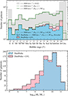 |
Fig. 1. Distributions of the morphological type (top panel) and stellar mass (bottom panel) of the galaxies in our study. Blue histograms represent the distributions of DustPedia galaxies, while the pink ones correspond to the DustPedia + LVL combined sample. In the top panel the HyperLEDA parent sample, from which DustPedia was selected, is plotted with a grey histogram. Changes in the distribution, due to further selection criteria (i.e. D25 > 1′ and W1-band above 5σ) are shown with a dashed and a solid green histogram, respectively. An extra bin includes morphologically unclassified (Unc.) sources. |
The DustPedia datasets for the 875 galaxies in the sample includes photometry executed in a systematic and uniform way across the following bands: GALaxy Evolution eXplorer (GALEX; Morrissey et al. 2007) FUV/NUV; Sloan Digital Sky Survey (SDSS; York et al. 2000; Eisenstein et al. 2011) ugriz; 2 Micron All-Sky Survey (2MASS; Skrutskie et al. 2006) JHKs; WISE 3.4, 4.6, 12, and 22 μm; Spitzer IRAC (3.6, 4.5, 5.8, and 8.0 μm) and MIPS (24, 70, 160 μm); Herschel PACS (70, 100, 160 μm; Poglitsch et al. 2010); and SPIRE (250, 350, 500 μm; Griffin et al. 2010). This process employed aperture-matched techniques, accompanied by comprehensive and compatible uncertainty calculations for all bands. Additional photometric data were taken from IRAS (12, 25, 60, and 100 μm) and from the Planck Surveyor (9 bands including 350, 550 and 850 μm; Planck Collaboration XXVI 2016). For a full description of the photometry pipeline, we refer the reader to Clark et al. (2018).
In this work, we limit the analysis to the objects for which physical properties were derived by Nersesian et al. (2019). Out of these 814 galaxies, 33% have an elliptical-lenticular morphology, 54% are spirals, and 13% are irregulars.
2.2. The Local Volume Legacy sample
The LVL survey provides a sample of 258 galaxies, fully representative of the nearby star-forming population. It consists of all known galaxies within 3.5 Mpc lying outside the Local Group and the Galactic plane (|b|> 20°), as well as galaxies in the M81 group and Sculptor filament. These are supplemented by a statistically representative outer tier – derived from the 11 Mpc Hα and Ultraviolet Galaxy Survey (Kennicutt et al. 2008) – that further consists of two subsets. The primary includes galaxies that meet a combined criterion of D ≤ 11 Mpc, |b|> 20°, mB < 15 mag, and T ≥ 0; the secondary consists of galaxies within 11 Mpc that fall outside one of the limits in Galactic latitude, magnitude, and morphology, but for which there are available Hα data. Out of these, for the LVL outer tier the ones with |b|> 30° and mB < 15.5 mag are selected, and they reach a completeness of 95% (Lee et al. 2009). The median distance of the galaxies in LVL is 5.9 Mpc, with the majority of them lying between 0.5 Mpc and 11 Mpc. Dwarf systems constitute 75% of the sample. The LVL survey includes observations from the FUV up to 160 μm, i.e. GALEX FUV/NUV, integrated narrow-band Hα line flux corrected for N II emission by Kennicutt et al. (2008), UBVRCIC, SDSS ugriz, 2MASS JHKS, Spitzer IRAC (3.6, 4.5, 5.8, 8.0 μm) and MIPS (24, 70, 160 μm), and IRAS (12, 25, 60, 100 μm), if available. The photometry was performed carefully, with the same aperture size being used across all wavelengths and all of the observable emission being captured (for a detailed description of the survey, photometry, and flux properties of the sample see Dale et al. 2009).
Physical properties were derived by Dale et al. (2023) for the 255 LVL galaxies with sufficient photometric coverage; of these, 58 are also included among the DustPedia objects analysed by Nersesian et al. (2019). Apart from the tests in Appendix A, we removed the overlapping objects from LVL and considered them as part of DustPedia only. There are thus 197 independent LVL objects, mostly irregulars (61%) and spirals (31%). The rest (8%) are ellipticals and lenticulars.
Because of its morphological composition, LVL complements DustPedia with objects against which the latter was more biased (see Fig. 1, top panel). Anticipating the results of Sect. 4, we also show in Fig. 1 (bottom panel) that LVL is complementary to DustPedia in stellar mass as well.
2.3. Overlap with other samples
The combined DustPedia-LVL sample, consisting in total of 814 + 197 = 1011 objects, has a significant overlap with many of the Herschel-based samples with which we compare our results: 272 galaxies are part of HRS (∼84% of that sample); 53 are among the 61 objects in the Key Insights on Nearby Galaxies – a Far-Infrared Survey with Herschel (KINGFISH; Kennicutt et al. 2011) project (∼87% of the sample); 17 are part of the Dwarf Galaxy Sample (DGS; Rémy-Ruyer et al. 2013, made of 48 galaxies, thus ∼35% of overlap); 16 are among the 42 galaxies in the Herschel-ATLAS Phase-1 Limited-Extent Spatial Survey (HAPLESS; Clark et al. 2015); and 16 are among the H I-selected Galaxies in H-ATLAS sample (H IGH; De Vis et al. 2017a, 39% of its 41 objects), including 5 in the H IGH-low sub-sample of galaxies with log10(M*/M⊙) < 9.0. Apart from a few LVL galaxies, almost all of the overlap is with DustPedia, because of its construction from the post-mission Herschel Science Archive. Chastenet et al. (2025) recently published another sample based on the Herschel Science Archive, collecting FIR-submm data for 877 local galaxies within ∼50 Mpc belonging to the z = 0 Multiwavelength Galaxy Synthesis project (z0MGS; Leroy et al. 2019); about half of these, 448 galaxies, are in common with our combined sample. There is instead no overlap between DustPedia-LVL and the 193 JINGLE galaxies, because of the mutually exclusive limits in distance selection.
The samples listed in this section contain only a limited number of objects with M* ≲ 109 M⊙, just as DustPedia alone does. Only LVL provides access to a larger number of low stellar-mass galaxies.
3. SED fitting
The multi-wavelength photometry of DustPedia and LVL facilitates the derivation of the galaxies’ physical properties, through a SED-fitting analysis: using this approach, the physical properties of the DustPedia galaxies were derived by Nersesian et al. (2019), and those of LVL by Dale et al. (2023); the CIGALE SED-fitting code (Boquien et al. 2019) was used in both studies. After setting a grid of values for the parameters defining the various modules for the emission by stars, gas, dust, and the dust attenuation, CIGALE generates a library of model-SEDs and through Bayesian inference assesses which model SED best fits the observations. This procedure is performed under the assumption that the energy absorbed and then re-emitted by dust particles is fully conserved. Several modules are available for each component in CIGALE and the estimated physical properties might differ by using different modules or by selecting different values for the free parameters of each module.
The parameter space employed in estimating the physical properties of the DustPedia galaxies is described in detail by Nersesian et al. (2019). We briefly mention the parameters’ set-up below. A flexible-delayed SFH, which allows a late burst or quenching event at 200 Myr before the current moment (module ‘sfhdelayedbq’; see Ciesla et al. 2015), is assumed, with the age of the galaxy varying between 2 and 12 Gyr. The Bruzual & Charlot (2003, BC03) single stellar population module of fixed (solar) metallicity is coupled to the Salpeter (1955) initial mass function (IMF). For the nebular line and continuum emission, the default set, which is based on CLOUDY templates (Ferland et al. 2013; Inoue 2011), is used. The stellar and nebular emission are attenuated using the same power-law-modified starburst attenuation curve derived by Calzetti et al. (2000) and extended by Leitherer et al. (2002, module ‘dustatt_calzleit’). The dust emission modules are estimated using the Heterogeneous dust Evolution Model for Interstellar Solids (THEMIS; Jones et al. 2017), composed of grains of amorphous (hydro)carbons (a-C, a-C:H) and amorphous silicates with Fe inclusions, whose optical properties are firmly based on laboratory measurements (Jones 2012a,b,c, 2013, 2017; Köhler et al. 2014). In our study we have nine free parameters and a total of about 8 × 10⁷ models were produced. The grid of parameters used is listed in Table 1 of Nersesian et al. (2019).
The SEDs of LVL galaxies were fitted by Dale et al. (2023) using the same CIGALE modules as Nersesian et al. (2019) for the SFH, stellar libraries, and dust attenuation. However, they used a different IMF (Chabrier 2003), dust emission module (based on the emission templates of Draine et al. 2014), and parameter grid, with 11 free parameters and about 3.4 × 10⁹ models. For the sake of uniformity, we repeated the fitting using the same parameter space and dust model used for DustPedia. Since the LVL data provided by Dale et al. (2023) have not been corrected for foreground Galactic extinction, we corrected the fluxes in all bands shorter than λ < 10 μm, following the methodology presented in Clark et al. (2018). Upper limits in flux were included in the using the default ‘noscaling’ option of CIGALE.
Nersesian et al. (2019) find that in 19 DustPedia galaxies the infrared flux might be contaminated by a strong active galactic nucleus (AGN), according to WISE colours and the Assef et al. (2018) 90%-confidence criterion; however, those objects do not have a SED substantially different from that of galaxies of the same bolometric luminosity (Bianchi et al. 2018). Using Spitzer-IRAC photometry and the criterion of Donley et al. (2012), we find only one LVL galaxy (NGC 5253) that might host a strong AGN. From the van Velzen et al. (2012) catalogue, Nersesian et al. (2019) selected four more DustPedia objects whose FIR SED might be contaminated by synchrotron and free-free emission from radio lobes (there are no LVL objects matching this selection). Given their limited numbers (23 DustPedia plus 1 LVL galaxies), our results cannot be biased by these objects. Thus, we follow the previous analysis and do not use any CIGALE module to fit the contribution of AGNs and radio-lobes; we only mark the objects with different symbols in some of the plots.
From our CIGALE fits for LVL galaxies, we used in this work the estimates for M*, Mdust, and SFR (and thus, sMdust and sSFR) together with their errors (typically larger for Mdust and SFR than for M*). In Appendix A we show that our results are compatible with those presented by Dale et al. (2023), once the difference in parametrisation is taken into account, and that the lack of FIR-submm data for λ > 160 μm does not bias strongly the results for LVL galaxies.
4. Scaling laws of specific dust mass
Dust is formed by metals that are synthesised in stars and both the formation and destruction of the grains is connected to the life cycle of stars. Moreover, it is found that the sMdust can be used as an observational proxy of the molecular gas fraction (see e.g. Rémy-Ruyer et al. 2014; Magdis et al. 2021) and of the total gas reservoir (Corbelli et al. 2012; Orellana et al. 2017; Casasola et al. 2020; Salvestrini et al. 2025; Paspaliaris et al. 2025). Thus, the dust content relates closely to the stellar mass and the star formation activity in galaxies and the sMdust serves as a valuable tool towards understanding the dust production mechanisms and generally the evolution of the ISM in galaxies (see also Calura et al. 2017). In this section we show the results of the homogeneous SED fitting of the combined DustPedia-LVL sample. In particular, we present sMdust as a function of M* and of the sSFR; the latter can also be considered as a proxy of the gas fraction in a galaxy, since the SFR is regulated by the available gas reservoir as indicated by the gas-SFR relation (i.e. the Kennicutt-Schmidt relation; Kennicutt 1998; see also da Cunha et al. 2010; Berta et al. 2016; De Looze et al. 2020). Since in general M* increases with a galaxy’s age, and the amount of gas relative to stars decreases (because of astration), the trends of sMdust with M* and (decreasing) sSFR have been interpreted as an evolutionary sequence for the dust content in galaxies (Cortese et al. 2012; Rémy-Ruyer et al. 2015; Calura et al. 2017; De Vis et al. 2017b; De Looze et al. 2020; De Vis et al. 2021; Galliano et al. 2021).
4.1. sMdust versus M*
In Fig. 2 we plot log10(sMdust) as a function of log10(M*). For the sake of presentation, we divided the galaxies according to the uncertainty of the estimates: if an object has σ(log10(sMdust)) > 0.22 (i.e. S/N =sMdust/σ(sMdust) < 2), it is shown with an open circle; the same criterion was applied to the uncertainty on M*, even though it is sMdust that dominates the selection. The median error bars of the two uncertainty ranges are shown in the plot. Out of the 1011 objects in the combined sample, 455 objects have more uncertain estimates: most of them are ellipticals, lenticulars, and irregulars (90.5%, 69.5%, and 68.6%, respectively), with smaller fractions for the other morphological types (15.8% for Sa-Sab, 8.7% for Sb-Sc, and 28.3% for Scd-Sdm). Despite the large uncertainties, these estimates are nevertheless useful when trends are studied over several orders of magnitude. Figure 2 also highlights with different colours the sample to which a galaxy belongs (either DustPedia or LVL; left panel) and its morphological type (right panel). In order to better visualise the trends with morphology, we fitted a fifth-order polynomial to M* and sMdust as a function of the Hubble stage, T (see Appendix B); the two fits are combined and plotted in the right panel of Fig. 2, colour-coded by morphological type.
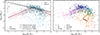 |
Fig. 2. sMdust as a function of M*. In the left panel DustPedia and LVL galaxies are shown in blue and pink, respectively; in the right panel galaxies are colour-coded with morphology. Objects are divided between those with larger (open and paler circles) and smaller uncertainties (filled and darker circles; see text for details): the black error bars in the left panel show the median values of the uncertainties in both ranges. In the left panel, the dashed red curve is the smoothly joined bilinear fit for LTGs, the shaded area shows the dispersion around the fit, and the two paler dashed curves indicate the fitted intrinsic scatter. We also show the fits by Casasola et al. (2020) and De Looze et al. (2020), and mark galaxies hosting AGNs or s radio jet with a ‘x’ or a ‘+’ symbol, respectively (see Sect. 3). In the right panel, the coloured curve shows the combination of the fitted fifth-order polynomials, of each physical property, parametrised with Hubble stage (from T = −5 to T = 10; pink to dark-red; see Table B.1) on the sMdust–M* plane. The uncertainty of the polynomials is indicated by the shaded grey area. |
The left panel of Fig. 2 confirms visually what we anticipated in Sect. 2.2 and Fig. 1. The LVL and DustPedia are complementary not only in morphologies, but also in stellar masses. The bulk of the DustPedia galaxies have 8 < log10(M*/M⊙) < 11, with a median value of 9.75, while the majority of the LVL galaxies have lower stellar masses, with 6.5 < log10(M*/M⊙) < 9.5 and a median value of 8.19. Figure 2 also shows that the trends for the low and high M* ranges are different: sMdust increases with M* for lower stellar masses, reaching a peak at log10(M∗/M⊙) ≈ 9.5, beyond which the trend is reversed. The galaxies along the increasing trend are mainly Sm-Irr, with fewer Scd-Sdms (the majority being LVL objects), while the remaining morphological types follow the decreasing trend (and are mostly from DustPedia), with the early-types (E, S0) being distinct from the spirals (Sa-Sdm) and more scattered. The Spearman’s correlation coefficients in both mass ranges are very similar (in terms of the absolute value): we obtain ρS = 0.43 when selecting galaxies with log10(M*/M⊙) < 9.5, ρS = −0.45 for log(M*/M⊙) > 9.5; this rises to ρS = 0.57 and −0.56 for the two stellar mass ranges, respectively, when only LTGs (T > 0.5) are considered. While the negative correlation for high stellar masses is well established in the literature, as we discuss later, the positive correlation for the low-mass end echoes that found by Dale et al. (2023) using LVL data only, i.e. the motivation for the current work. The correlation claimed by those authors, ρS = 0.58 (without any cut in morphology), is stronger than what is measured here, probably because of the exclusion of those galaxies for which they only provide upper limits in Mdust.
We used the Python UltraNest package for Bayesian inference (Buchner 2021) to fit the data points with a function that smoothly joins, at intermediate stellar masses, a negative and a positive linear correlation, i.e.
 (1)
(1)
The intrinsic scatter of the data points, σ, was also fitted. The fit considers errors on both axes, for all data points, regardless of the error magnitude. When selecting only LTGs, we obtain
Results of the fit are shown in the left panel of Fig. 2, in which we plot the median representation of the model, together with the dispersion given by the 0.16 and 0.84 percentiles around the median, and the intrinsic scatter. While the parameter defining the smoothing, ϵ, is poorly constrained, those for the two linear correlations are very similar to what would have been obtained by separately fitting the data points below and above log(M*/M⊙) = 9.5 (which is also close to the position of the maximum of the joining function). When all morphological types are considered, instead, the slope will become flatter for galaxies with lower stellar masses, and steeper (in absolute value) for higher stellar masses (not shown), as a result of the lower (and more uncertain) values of log10(sMdust) for early-type galaxies (ETGs), and of their general negative correlation with log10(M*). Correlations and fits for each morphological type are shown in Appendix B.
4.2. sMdust versus sSFR
In Fig. 3 we plot log10(sMdust) as a function of log10(sSFR). In analogy with Fig. 2, data points are colour-coded by sample (left panel) and morphology (right panel); open circles are used for galaxies with uncertain estimates. In this plot, the uncertainty for the quantity on the y axis, sSFR, can also be significant. Thus, defining objects with uncertain estimates, those with S/N < 2 for sMdust or sSFR, results in a larger selection. There are now 557 of these galaxies (97.3% of all E, 85.7% of S0, 46.3% of Sa-Sab, 20.8% of Sb-Sc, 31.2% of Scd-Sdm, and 70.0% of Sm-Irr galaxies). Also, galaxies that were considered to have more certain estimates in Fig. 2, because they have S/N > 2 for sMdust, could be classified as uncertain in Fig. 3 because they have S/N < 2 for sSFR; this is reflected in the different median error bars in Figs. 2 and 3.
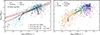 |
Fig. 3. sMdust as a function of sSFR. The colours and shapes, median error bars, and marks indicating AGNs and radio jets (left panel) are the same as in Fig. 2. In the left panel, the dashed red curve is the linear fit to LTGs with log10(M*/M⊙) > 9.5, the shaded area the 1σ dispersion around the fit, and the two paler dashed curves the fitted intrinsic scatter (the short-dashed line being the fit including also ETGs). The dotted line is the fit by De Looze et al. (2020). The black squares show the median, and standard deviation, for bins in M* of 1.0 dex width, centred from log10(M*/M⊙) = 7 (on the right side of the panel) to log10(M*/M⊙) = 12 (on the left side). In the right panel, the coloured curve shows the combination of the fitted fifth-order polynomials, of each physical property, parametrised with Hubble stage (from T = −5 to T = 10; pink to dark red; see Table B.1) on the sMdust–sSFR plane. The uncertainty of the polynomials is indicated by the shaded grey area. |
Figure 3 shows that log10(sMdust) in general increases with increasing sSFR, with most of the objects from DustPedia following the increasing trend, while those of LVL are mostly below it, dragging the trend at lower sMdust for high sSFR. Indeed, most LVL galaxies have similar log10(sSFR/yr−1) values, of between −10.2 and −9.2, but a wide spread of log10(sMdust) values, from −2.8 to −4.5. This trend becomes evident when we plot the running median of all DustPedia-LVL galaxies in bins of log10(M*/M⊙). Galaxies of lower M* have a higher sSFR. As we have also seen in Fig. 2, while M* increases, sMdust increases until it reaches a peak, at log10(sSFR/yr−1)≃ − 9.9; this happens with a small variation (< 0.5 dex) in log10(sSFR). Going towards the highest M* bins, both the sMdust and the sSFR decrease. The right panel of Fig. 3 shows that the place where galaxies lie in the diagram also depends on their morphology. For instance, although Sm-Irr galaxies have similar sSFRs as the late spirals (Scd-Sdm), they have lower sMdust, in accordance with their lower M*. Similarly to the trend suggested by the stellar mass bins, the combination of the fitted fifth-order polynomials of the plotted properties (see Appendix B) shows the sMdust rapidly increasing with a relatively constant sSFR for the Sm-Irr and Scd-Sdm bins. In this case the peak sMdust occurs at a slightly higher log10(sSFR/yr−1(= − 9.8). The sMdust then decreases with decreasing sSFR for earlier-stage galaxies.
The correlation between log10(sMdust) and log10(sSFR) for all objects has Spearman’s coefficient, ρS = 0.62. Because of what we discussed in the previous paragraph, the significance of the correlation increases when the sample is restricted to galaxies with log10(M*/M⊙) > 9.5: in this case we have ρS = 0.85 (for 525 objects; equivalent results can be obtained by selecting DustPedia galaxies only). A fit to these objects (red line, small dashes; Fig. 3, left panel) yields
 (2)
(2)
with an intrinsic scatter of σ = 0.27 ± 0.01 dex. If we restrict the fit to the massive LTGs (T > 0.5, 321 objects) only (red line; long dashes), we get
 (3)
(3)
with a reduced intrinsic scatter, σ = 0.20 ± 0.01 dex; the correlation coefficient, however, is smaller, ρS = 0.65, because of the more restricted dynamic range of log10(sSFR). When fits are done for individual morphology bins (Appendix B), a positive trend is found in all cases, again with different normalisations and intrinsic scatter: the smallest scatter is for Sa-Sab and Sb-Sc. It becomes larger for Sm-Irr, whose fit is below that of the later-type spirals, in accordance with what has been discussed so far, and it is largest for ellipticals.
4.3. Comparison with previous works
The negative correlation between log10(sMdust) and log10(M*) at higher stellar masses, shown in Fig. 2, is a well-known result in the literature and has been found for a wide diversity of samples of galaxies in the local Universe. For instance, it has been described for HRS (Cortese et al. 2012), for the Planck-selected sample of Clemens et al. (2013), for the JINGLE sample, united with HRS, KINGFISH, HAPLESS and H IGH (De Looze et al. 2020), and for the LTGs in DustPedia (Casasola et al. 2020). Only Chastenet et al. (2025) find no correlation for the z0MGS galaxies they study but, as they admit, this is mainly due to the exclusion of objects with low sSFR from the analysis. The normalisation and the slope of the correlation are found to vary depending on various selections; for instance, Cortese et al. (2012) and De Looze et al. (2020) find that sMdust is systematically lower for HI-deficient galaxies, while Orellana et al. (2017) – using a sample of 1630 galaxies with an Planck detection – derived a steeper correlation for starbursts than for more quiescent ones. The inverse correlation was confirmed by Donevski et al. (2020) on a more distant sample (up to z ≃ 5), but with a median sMdust more than an order of magnitude higher than those of local ETGs and LTGs, indicating an evolution with redshift. Two fits from the literature are shown in Fig. 2: that of Casasola et al. (2020), obtained for DustPedia LTGs with the same CIGALE dataset as was used in this work; and that of De Looze et al. (2020) for their JINGLE-based sample (corrected for their different modelling parametrisation; see Appendix C). The two fits are fully compatible with each other. Since the range of their analyses extends to lower M*, their fitted linear trends are flatter than what is obtained here for high M* only, but overall consistent with the current results.
Instead, the positive trend of sMdust versus M*, for low M*, has only been described in a few literature works and required carefully crafted samples, because of the difficulty of estimating the properties for low-mass galaxies. Grossi et al. (2015) studied the star-forming dwarfs in the Herschel Virgo Cluster Survey (HeViCS; Auld et al. 2013), combined with similar objects from KINGFISH and DGS, and found hints of a change in trend with respect to more massive KINGFISH and HeViCS galaxies, but with a large scatter that prevented the detection of any correlation. De Vis et al. (2017a), studying 17 galaxies with log10(M*/M⊙) < 9 (the H IGH-low sample), find a different trend with respect to more massive objects. Suggestions for a change in slope at small M* can also be found in other samples (see, for example, Fig. 11 in Casasola et al. 2020 and Fig. 2 in De Looze et al. 2020 for log10(M*/M⊙) < 9), again for a limited number of objects.
The strong correlation between log10(sMdust) and log10(sSFR) shown in Fig. 3 was already found by da Cunha et al. (2010), with ρS = 0.84 for a sample of ∼3200 galaxies; they also demonstrated that this is not driven by the M* (used at the denominator of both the sMdust and sSFR). The correlation has been confirmed for several Herschel-based samples: for HRS, by Cortese et al. (2012), using NUV-r as proxy for sSFR; for KINGFISH (Rémy-Ruyer et al. 2015); for HRS, HAPLESS, and H IGH (De Vis et al. 2017a); for those samples above, plus JINGLE (De Looze et al. 2020); and for DustPedia and the DGS (Galliano et al. 2021). The De Looze et al. (2020) fit, including galaxies of all morphological types, is shown in the left panel of Fig. 3 (after the corrections described in Appendix C); it is analogous to what we find in this work without a morphological selection. While the paucity of objects in the local Universe prevents us from extending the analysis at log10(sSFR/yr−1) > − 9.4, we note here that samples of high-redshift galaxies have shown that the general correlation of log10(sMdust) and log10(sSFR) extends beyond that limit (Rowlands et al. 2014; De Vis et al. 2017a; Donevski et al. 2020).
Also for log10(sMdust) versus log10(sSFR), the departure of galaxies of lower stellar mass from the main scaling law of Fig. 3 has been found and described only for a few samples of galaxies with specific properties. For similar values of sSFR, De Vis et al. (2017a) find lower sMdust than the main trend for the HiGH-low galaxies. Another sample showing no significant correlation between sMdust and sSFR is the DGS, made up of 48 star-forming and low-metallicity dwarfs that have lower sMdust and higher sSFRs than expected from the trend shown by KINGFISH galaxies (see Fig. 11 in Rémy-Ruyer et al. 2015).
4.4. Advantages and caveats
We have shown in this section that the combination of LVL and DustPedia allows one to study the main scaling laws of sMdust, and the departures from them for different galaxy subsets, in more detail than what was previously possible by including a small number of low-mass objects in larger samples of more massive galaxies. For example, De Vis et al. (2017a) did not attempt to fit the sMdust versus M* trend because of the small number of objects in their H IGH-low sample of 17 galaxies with log10(M*/M⊙) < 9. DustPedia-LVL, instead, contains 309 galaxies in the same M* range; thus, we could also fit the low-mass regime. Similarly, Galliano et al. (2021) studied the evolution of dust by supplementing DustPedia with 34 DGS objects, while LVL adds 197 objects to the larger sample.
However, a caveat for the use of LVL should be mentioned, i.e. the lack of FIR/submm data for λ> 160 μm. In Appendix A we discuss the possibility of an underestimate of Mdust (and thus of sMdust): if we correct the dust masses of LVL galaxies according to the (rather uncertain) fit shown in Fig. A.2, low-M* galaxies will show a shallower trend of log10(sMdust) versus log10(M*) than that presented in Fig. 2, with Spearman’s ρS = 0.3; yet the dichotomy with the trend of high M★ galaxies (unaltered by the correction) will remain. Similarly, the difference between sMdust for high- and low-M* galaxies at high sSFR will remain, though much reduced. Currently, LVL galaxies with log10(sSFR/yr−1)≈ − 10 and log10(M*/M⊙)≈8 have sMdust values 0.8 dex lower than their log10(M*/M⊙) > 9.5 counterparts; this will reduce to just 0.2 dex after the correction. Future FIR/submm observations of LVL galaxies beyond the peak of thermal emission are needed to settle this issue.
5. Dust evolution modelling
Several works have modelled the variation in the dust content (and other integrated properties) of galaxies as a function of cosmic time (e.g. Dwek & Scalo 1980; Dwek 1998; Lisenfeld & Ferrara 1998; Hirashita 1999; Morgan & Edmunds 2003; Inoue 2003; Dwek et al. 2007; Galliano et al. 2008; Calura et al. 2008; Valiante et al. 2009; Mattsson & Andersen 2012; Asano et al. 2013; Zhukovska 2014; Feldmann 2015; De Looze et al. 2020; Nanni et al. 2020; De Vis et al. 2021; Sawant et al. 2025). In particular, limited samples of galaxies of low stellar mass (i.e. H IGH and DGS) have been used to define the earlier stages of dust evolution (De Vis et al. 2017b; Galliano et al. 2021).
In this section we explore the impact of the DustPedia-LVL dataset on dust modelling, and in particular of the estimates for the larger number of low-stellar mass galaxies available from LVL. We first compare the scaling laws presented in the previous section with published evolutionary models; we then use the chemevol5 (De Vis et al. 2021) to understand which parameters for dust evolution can better describe the dataset presented here.
5.1. Models from literature
We first compare the DustPedia-LVL results with four models for sMdust we selected from the literature: Calura et al. (2009, Ca09), whose estimations for sMdust, M*, and sSFR for spiral galaxies of three different baryonic masses (Mbar) are taken from Calura et al. (2017), Asano et al. (2013, As13), whose estimations for sMdust versus sSFR, for a total baryon mass (stars+ISM) of 1010 M⊙ and three different star formation timescales (τSF; i.e. the ISM depletion timescale), are taken from Rémy-Ruyer et al. (2015, the trend vs. M* is not available); the models of Galliano et al. (2021, Ga21) for an initial gas mass of 4 × 10¹⁰ M⊙ and three different outflow rates, presented in their Fig. 15; the results of hydrodynamical simulations of isolated disc galaxies by Richings et al. (2022, Ri22; only sMdust vs. M* is presented by the authors), with M*, tot ranging from 6.6 × 10⁶ M⊙ (dwarfs) to 3.1 × 10¹² M⊙ (massive galaxies), in five steps, with two additional cases in which the gas fraction is increased (or decreased) by 20%, for M∗,tot = 1.1 × 10¹⁰ M⊙, but without a dust evolution model included; and the dwarf mass (sub-Small Magellanic Cloud to Large Magellanic Cloud) to Milky Way simulations (Choban et al. 2024, Ch24), which include a dust evolution model with a constant grain size (Choban et al. 2022).
The evolution frameworks developed by Ca09 and As13 incorporate the same fundamental physical mechanisms: dust formation in the ejecta of core-collapse SN and AGB stars, subsequent grain growth in the dense ISM, and dust removal through SN-driven destruction and astration. Their treatments diverge primarily in the environmental regulation of these processes. In the Ca09 model, the spiral galaxy is dominated by a thin disc of stars and gas, consisting of several independent rings without exchange of matter among them. They adopted an inside-out disc formation, with the timescale for disc formation increasing with galactocentric distance, and assumed that the star formation efficiency (SFE) is higher for more massive objects. As13 employed a closed-box model that isolates the intrinsic interplay between stellar dust production and accretion, allowing them to identify the critical metallicity, above which grain growth becomes the dominant channel. Ga21 rewrote the chemevol version of De Vis et al. (2017b), which adopts the same physical mechanisms as the two aforementioned models (i.e. Ca09, As13) for dust production and destruction, but embedded these processes within a more dynamically realistic context that includes gas inflows, outflows, and galactic fountains (i.e. recycling of the outflows), each of which can dilute, expel, or destroy dust and thereby modulate the efficiency and timing of the underlying mechanisms. In their version, Ga21 extended the code’s formalism by applying a hierarchical Bayesian framework to constrain the efficiencies of SN dust condensation, grain growth, and shock destruction across a large sample of galaxies. The Ri22 models were computed with the hydrodynamics code GIZMO (Hopkins 2015), assuming a rotating disc of gas and stars, along with a spherical central stellar bulge, all embedded within a live dark matter halo. The parameters of the models (e.g. bulge-to-total ratio, half-light radius, gas fraction, and metallicity) were accordingly chosen in order to follow the scaling relations of nearby typical spiral galaxies at redshift zero. Within the simulations other processes are implemented, such as star formation and feedback by SN, stellar winds, photoionisation of the surrounding gas, and stellar radiation pressure, as well as non-equilibrium chemistry covering a wide range of gas phases, from cold dense molecular clouds to hot highly ionised plasma. By also using GIZMO within the Feedback in Realistic Environments (FIRE) project, the Ch24 models track the non-equilibrium evolution of dust grains of multiple species (e.g. carbonaceous, silicates, iron), accounting for their production, growth, and destruction.
The comparison between DustPedia-LVL and the literature models is shown in Fig. 4. We note that, while we fitted galactic properties adopting the Salpeter (1955) IMF, this is used by Ga21 only; instead, Ca09 adopt Scalo (1986), As13 Larson (1998), Ri22 and Cho24, Kroupa (2001). Unfortunately, conversion factors are not available in the literature between Salpeter (1955), typically producing higher values for M* and SFR, and all the other IMFs above: if we had applied the conversion from the Kroupa (2001) IMF (as in Madau & Dickinson 2014), and if conversion from other IMFs is similar, the modelled sMdust would have been about 0.2 dex lower and M* 0.2 dex higher (and sSFR almost unchanged), i.e. by about a symbol size for models in Fig. 4. Furthermore, other different assumptions on galactic modelling might have resulted in other shifts (see Appendices A and C). Thus, we apply no correction but keep in mind that possible offsets between models and between a model and our results might be due to this issue. Looking at the log10(sMdust)–log10(M*) plane (left panel of Fig. 4), the Ca09 model follows the negative trend for higher M*, found for our data (apart from a systematic offset towards higher sMdust values). The Ga21 models show that for the same M*, galaxies exhibiting stronger outflows ultimately display lower sMdust, providing an interpretation for the high dispersion that we find in the high M* regime. Similarly, the sMdust trend with M* of the Ri22 and Ch24 simulated galaxies is in good agreement with our observed galaxies (especially if we apply the corrections expected for Kroupa 2001). However, while Ch24 models predict low sMdust values in the low-M* regime, a larger difference is found by Ri22. This could be attributed to higher gas fractions assumed by the models compared to the ones in the observed sample, as is suggested also by their more massive models showing that the dispersion of the sMdust for a specific M* depends on the gas content of the galaxies. Specifically, for their galaxies with log10(M∗/M⊙) ≃ 10 they find different sMdust by assuming different gas fraction. Regarding log10(sMdust) versus log10(sSFR), shown in the right panel of Fig. 4, apart from the Ch24 models, all the rest show a larger dispersion than the one suggested by our data. The As13 model with the lowest τSF lies on top of our data, while higher τSF gives higher sMdust than what we find. Similar sMdust is predicted by the Ca09 dwarf galaxy model. On the other hand, the higher-mass Ca09 models are in better agreement with our data, following, though, a steeper decrease in sMdust as we go to higher masses (lower sSFR) than that found for our sample. The Ga21 models do not agree with our data in the log10(sMdust)–log10(sSFR) plane; however, we need to stress out that as stated by them this might reflect a simplistic SFH, outflow, and inflow prescription used in their models. For this reason, we present the properties of models with lower outflow rates, at 10 Gyr, as at later ages they give a very small sSFR for a constant sMdust, and the ones of the model with high outflow rates, at only 4.6 Gyr, since after that age it runs out of ISM.
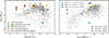 |
Fig. 4. sMdust as a function of M* (left panel) and sSFR (right panel), compared to model predictions from the literature. Galaxies with uncertain estimates are shown with open symbols. Model estimates by Galliano et al. (2021, Ga21) are shown with blue squares; the lighter blue colour corresponds to a higher outflow rate (δout). The models for three spiral galaxies of different baryonic masses from Calura et al. (2009, Ca09) are plotted with green diamonds, with darker green indicating a higher assumed baryonic mass. Predictions for isolated disc galaxies by the Richings et al. (2022, Ri22) and FIRE (Choban et al. 2024, Ch24) simulations are also plotted in the left panel, with orange and yellow, respectively. In the right panel, together with the Ca09, Ga21, and Ch24 estimations, the predictions of Asano et al. (2013, As13) are also plotted with violet hexagons; lighter colours represent higher star formation timescales (τSF). Predictions by Ri22 for the right panel, and by As13 for the left panel, are not available in the literature. Galaxy age of the models is equal to 13 Gyr if not indicated. |
5.2. Our evolutionary models estimated with chemevol
The comparison of our observed galaxies with the model predictions from the literature indicates that different model assumptions and initial conditions can lead to different results. In the following, we use chemevol to study the dependence of the observed trends on the various parameter models and we investigate how the combined DustPedia-LVL data can help to constrain the properties of the models.
We already mentioned some details of chemevol above, but here we describe the basic features of the model. The code solves differential equations that account for the secular evolution of the main building blocks of galaxies, i.e. stars, gas, heavy elements, and dust, under the assumption that they are perfectly mixed. The ISM is separated into clouds and diffuse ISM. Stars form from gas (pristine clouds initially), a portion of which is returned into the ISM at the end of their lifetimes. The model follows the stellar evolution as a function of the mass, which determines both the lifespan and the yields of elements and dust. The stellar component is strongly dependent on the IMF that is assumed. Gas is consumed through processes, such as astration and galactic outflows, while it is replenished via stellar feedback and inflow of metal- and dust-free gas. Heavy elements are infused in the ISM at the end of the stellar lifetime. A part of them returns into stars through astration and a fraction is lost through outflows. Dust is produced by three main processes: the condensation of elements into solid grains occurring in low- and intermediate-mass stars’ ejecta, the condensation in type-II SN ejecta, and grain growth through accretion from elements in the ISM.
For our investigation, we used as a reference the De Vis et al. (2021, DV21) best-fit model, assuming three initial gas masses (Mgas, init), aiming to cover the mass range of our combined sample. For each Mgas, init we assumed three start times (tstart) in order to estimate the properties of both younger and more evolved galaxies. The end time of the models was always fixed to 13.8 Gyr. Consistently with our CIGALE analysis, the best-fit model used a Salpeter (1955) IMF, the THEMIS dust model was adopted, and a delayed SFH was assumed. The SFH prescription adopted by DV21 is given by
 (4)
(4)
where z is the redshift, Mgas is the gas mass, and SFE0 is the reference SFE, which is a free parameter. As shown by DV21 (see their Sect. 3.3 for details), from the above empirical prescription the resulting SFH is consistent with the delayed SFHs observed in other works. We varied the key parameters of the model within their suggested rate (as listed in Table 1 of DV21). The reference model (denoted as ref) and its variations are shown in Fig. 5. The parameters investigated are listed in Table 1.
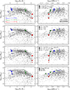 |
Fig. 5. sMdust as a function of M* (left panels) and sSFR (right panels) compared to our model predictions using chemevol. The colour-coding of data points is the same as in Fig. 4. Model estimates are colour-coded by Mgas, init, with darker colours corresponding to older galaxies (with a larger galaxy age, tgal). Apart from Mgas, init and tgal, in each row we also vary and indicate with a different symbol (i.e. circle, square, and triangle): the cold gas fraction (fc) and the outflow reduction factor (fout; first row), the THEMIS photofragmentation rate of a-C:H/a-C grains (kfrag; second row), both kfrag and the cloud grain growth scaling factor from THEMIS (kgg, cloud; third row), and the reference SFE (fourth row). Solid black lines correspond to the isochrones. |
Dust evolution parameter grid in chemevol.
5.3. Qualitative inspection of dust evolution parameters
In this investigation, for each parameter configuration, our starting point is the assumption of three Mgas, init values and two ages (tgal). As can be seen in the top panels of Fig. 5 the initial gas budget has the most significant effect on the present-day position of galaxies on both the planes studied. A larger assumed Mgas, init supplies additional material for galaxies, facilitating the attainment of higher stellar mass. In our models, half of the adopted initial gas mass is assumed to be in the form of inflows. If we vary this fraction (not shown here), we observe exactly the same behaviour as by varying Mgas, init. Moreover, younger galaxies (paler colours) with the same assumed model parameters systematically have lower M* (left panel) and higher sSFR (right panel). While in the log10(sMdust)–log10(M*) diagram the galaxy age leads to variation in the properties along both the x and y axes, in the log10(sMdust)–log10(sSFR) diagram, different galaxy ages correspond mainly to variations along the x axis.
A gas-related parameter (panels of first row) is the fraction of gas that lies in cold dense clouds (fc; default value is 0.5; As13). We see in the log10(sMdust)–log10(M*) plot that when the fraction is reduced to fc = 0.03 the galaxy ends up having the same M*, but slightly lower sMdust. The dependence of the sMdust variation on the fc, seems to be more significant at higher stellar masses (∼0.4 dex lower at log10(M∗/M⊙) ≃ 11), partially explaining the dispersion observed by our data in that regime. Similarly with the M*, in the log10(sMdust)–log10(sSFR) diagram, the fc does not affect the sSFR levels. In the same panels we also vary the outflow rates and specifically the outflows: reduce parameter (here fout). The outflow rates are defined by Nelson et al. (2019) and fout is not considered as a free parameter in DV21. The architecture of chemevol allows us to vary it though. We stress that fout is a factor that reduces the outflow rate, so by setting it below unity (e.g. 0.25 here), the outflow rate increases. So, when we increase the outflow rate we get galaxies with lower M* (by 0.1 to 0.3 dex, depending on Mgas, init), as expected, and lower sMdust (by ∼0.3 dex). Regarding the log10(sMdust)–log10(sSFR) correlation, lower-mass galaxies with a higher outflow rate have not only lower sMdust but also a slightly reduced sSFR. However, in the most massive galaxies, the outflows affect the sMdust more significantly, with their impact on the sSFR being negligible. Generally, fout affects all the physical properties examined here more significantly than fc, as it leads to a reduction in the ISM materials available for stellar and dust formation. A similar behaviour is observed by varying the outflow recycling time factor (not shown here). Longer recycling times lead to lower sMdust and M*. Among all the aforementioned models computed by varying gas-related parameters, the model for fout = 0.25 in intermediate- and low-mass galaxies is closer to the average values of our data in the log10(sMdust)–log10(sSFR) diagram. However, the gas-related parameters fail to reproduce low-mass galaxies with low sMdust, and high sSFR, as well as high-mass galaxies with low sMdust and sSFR, in each of the plots, respectively. This is apparent by the isochrones: the curves that cross the data points of galaxies with the same age and parameter configuration, but a different mass (see solid black lines in Fig. 5). The observed log10(sMdust)–log10(M*) trend of our data for log10(M*/M⊙)≳9 is reproduced by the isochrones; however, by varying gas-related parameters, we find that the models systematically overestimate the sMdust compared to the observed values for lower-mass galaxies. In the case of the log10(sMdust)–log10(sSFR) relation, the corresponding isochrones of both young and old low-mass galaxies follow the observed trend, and the massive galaxies deviate from it.
Apart from the gas-related properties, we also examined the effects of varying dust-related parameters. In the second row of panels we vary the THEMIS photofragmentation rate of large a-C:H/a-C grains (kfrag). We find that kfrag affects the youngest (7.8 Gyr old) and lowest stellar-mass galaxies. In such objects, the highest kfrag, 5.00, leads to lower dust content, reducing its sMdust by more than an order of magnitude. Young low-mass galaxies with high photofragmentation rates are the only ones that occupy the same area as is defined by our low-mass Sm-Irr galaxies, following the increasing trend in the log10(sMdust)–log10(M*) diagram, and lie in the low sMdust – high sSFR regime in the log10(sMdust)–log10(sSFR) diagram. Additionally, if we decrease the cloud grain-growth scaling factor, kgg, cloud, together with the increase in kfrag, the dust content varies more significantly, and a difference in sMdust is found, for the older low-mass galaxies as well as for the older high-mass ones (third row of panels in Fig. 5). Intermediate-mass galaxies are not significantly affected by either of the two aforementioned parameters. Another dust-related parameter that we explored is SNred, a factor that reduces the amount of dust that is formed in SN and reaches the ISM (for example, because it is destroyed by the reverse shock within the remnant; see, e.g. Bocchio et al. 2016). However, we do not plot it because SNred only affects the sMdust in the very early stages of a galaxy’s evolution, when SNe dominate dust production. At later stages, such as the ones we investigate, when grain growth in a higher-metallicity ISM is dominant, the properties are not affected by this factor.
Finally, as was mentioned already, the prescription of the adopted delayed SFH in Eq. (3) allows us to vary the SFE by assuming a different reference SFE0 (see Table 1). Hence, in the bottom panels of Fig. 5 we compute the models assuming various SFEs. We find that less massive galaxies are more sensitive to changes in the assumed SFE. As is suggested by the models, galaxies with a fast SFE attain a somewhat higher M* (up to 0.2 dex), and lower sMdust and sSFR (up to 0.5 dex and 0.7 dex, respectively), compared to their counterparts of the same age and an average SFE. The assumption of a slow SFE has the opposite effect. Massive galaxies [log10(M∗/M⊙) ≈ 11] are less affected by the various SFEs assumed.
Overall, the comparison between the properties of our observed galaxies and those of the theoretical models indicates that the observed log10(sMdust)–log10(M*) trend can be interpreted mainly by varying the initial gas mass in the models, while the log10(sMdust)–log10(sSFR) trend is mainly explained by varying galaxy ages. In general, while gas-related parameters similarly affect the galaxies, independent of their age and mass, low-mass galaxies, especially the younger ones, are more sensitive to differences in the dust-related model parameters. Intermediate-mass galaxies are the least sensitive to different dust-related assumptions and the properties of high-mass galaxies are not affected by the various assumed SFEs. The properties of our observed galaxies in the log10(M∗/M⊙) < 9 and log10(sSFR/yr−1) > −10 regimes can only be reproduced by modelled galaxies with tgal = 7.8 Gyr, high kfrag, and low kgg, cloud. The model cannot reproduce the observed sMdust for the latter subset if only gas-related properties or the SFE are varied. Taking into account the fact that in De Vis et al. (2017a) this regime is occupied only by their gas-rich low-stellar mass galaxies (HiGH-low subset), only variations in the dust-related properties can explain the trends for these objects (not only the initial low gas mass budget). Moreover, the ETGs (Es and S0s) could not be reproduced by any of the model configurations that we assumed. In general, the current exercise also highlights the diversity of galaxy evolution paths and the need for sophisticated galaxy-by-galaxy modelling approaches, as is also illustrated by Calura et al. (2023) with a model tailored to M74 (NGC0628, a DustPedia galaxy). The combined DustPedia-LVL sample can help direct how to constrain such models.
6. Summary and conclusions
We merged the DustPedia and LVL samples, obtaining a database of 1011 local galaxies. We estimated the physical properties of these galaxies through homogeneous SED fitting. We have shown that the combined sample includes galaxies of all morphological types, spanning a wide range of masses and star formation activity, well suited for studying the evolution of the dust content in the local Universe. Specifically, we studied the correlation of the sMdust as a function of M* and sSFR. Our main results are:
-
The trend of log10(sMdust) versus log10(M*) is not monotonic. A positive correlation is found for galaxies with log(M∗/M⊙) < 9.5, and a negative one for higher masses.
-
The peak of the sMdust in local galaxies, and the change in the slope of the correlation, occurs at log10(M*/M⊙) = 9.5.
-
The sSFR of high-mass galaxies establishes a strong linear correlation with sMdust. However, a large fraction of E and S0 sources lie below the linear trend, in the low-sSFR regime.
-
Low-mass spirals (Sa-Sdm), irregulars, and dwarf galaxies (Sm-Irr) lie in the high-sSFR regime, with an increased dispersion below the linear trend found for high-mass galaxies.
-
Grouping the galaxies in bins of stellar mass, we find that sMdust increases for low-mass galaxies that have a high sSFR, reaching a peak sMdust at log10(sSFR}/yr−1) ≃ −9.9. A similar behaviour is found by grouping the galaxies in bins of morphological type, with the peak occurring at 0.1 dex higher log10(sSFR).
We compared our results with evolutionary models provided in the literature and models that we computed using the one-zone dust evolution model of De Vis et al. (2021), by varying specific free parameters of their reference model. We find that:
-
The observed trends in the log10(sMdust)–log10(M*), and the log10(sMdust)–log10(sSFR) planes can be interpreted mainly as the result of different initial gas mass budget and different galaxy ages, respectively.
-
While gas-related parameters influence the positions of galaxies of all masses and ages in the examined diagrams, massive old galaxies are not sensitive to SFE variations. Dust-related parameters more significantly affect low-mass galaxies (especially the young ones) and the more massive old galaxies. The properties of intermediate-mass galaxies are not affected by the different assumptions of dust-related parameters.
-
The observed properties and trends of low-mass and highly star-forming Sm-Irr galaxies can be reproduced by the models if we assume a young galaxy age, a high efficiency for the photofragmentation rate of large grains, and/or a low grain-growth scaling factor in star-forming clouds.
The combination of DustPedia and LVL constitutes an ideal sample for studying dust evolution in nearby galaxies and could be used to constrain chemical evolution models. While a significant fraction of DustPedia galaxies have observations available for the atomic, molecular gas, and metallicity (De Vis et al. 2019; Casasola et al. 2020; Salvestrini et al. 2025), allowing further constraints to be set in evolutionary models (see, e.g. Galliano et al. 2021; De Vis et al. 2021), this is not the case for LVL. Future observations (or, possibly, literature compilations) of LVL galaxies, including H I 21 cm, 12CO emission lines, optical spectroscopy, and dust emission up to the submm, are needed to confirm and better interpret the scaling relations found in the current study. In particular, observations with the proposed PRobe far-Infrared Mission for Astrophysics (PRIMA6; Glenn et al. 2025) will help to better constrain their total dust budget and properties (see e.g. Casasola et al. 2025; Galliano et al. 2025).
Acknowledgments
We thank the anonymous referee, whose constructive comments and suggestions helped to clarify and improve the content of this study. We thank Daniela Calzetti, for drawing our attention to the “diversity” of the DustPedia and LVL results, and Médéric Boquien, for constructive discussions about CIGALE. EDP, SB, and EC, acknowledge financial support from INAF-Mini Grant 2024 program “Dust emission and optical extinction as gas tracers in star forming galaxies”. VC, SB, FC, FP, and VT acknowledge financial support from INAF-Mini Grant 2024 program “DustPedia meets Metal-THINGS: Dust-METAL”. EC acknowledges financial support from INAF-Mini Grant 2023 program “SHAPES”. VC, SB, FC, and FP acknowledge financial support from INAF-Mini Grant 2022 program “Face-to-Face with the Local Universe: ISM’s Empowerment (LOCAL)”. FG acknowledges support by the French National Research Agency under the contracts WIDENING (ANR-23-ESDIR-0004) and REDEEMING (ANR-24-CE31-2530), as well as by the Actions Thématiques “Physique et Chimie du Milieu Interstellaire” (PCMI) of CNRS/INSU, with INC and INP, and “Cosmologie et Galaxies” (ATCG) of CNRS/INSU, with INP and IN2P3, both programs being co-funded by CEA and CNES. DustPedia is a collaborative focused research project supported by the European Union under the Seventh Framework Programme (2007–2013) call (proposal no. 606824). The participating institutions are: Cardiff University, UK; National Observatory of Athens, Greece; Ghent University, Belgium; Université Paris-Sud, France; National Institute for Astrophysics, Italy and CEA (Paris), France. This research made use of Astropy (Astropy Collaboration 2013, 2018, 2022, http://www.astropy.org), matplotlib (Hunter 2007), NumPy (Harris et al. 2020), SciPy (Virtanen et al. 2020).
References
- Asano, R. S., Takeuchi, T. T., Hirashita, H., & Inoue, A. K. 2013, Earth Planets Space, 65, 213 [NASA ADS] [CrossRef] [Google Scholar]
- Assef, R. J., Stern, D., Noirot, G., et al. 2018, ApJS, 234, 23 [Google Scholar]
- Astropy Collaboration (Robitaille, T. P., et al.) 2013, A&A, 558, A33 [NASA ADS] [CrossRef] [EDP Sciences] [Google Scholar]
- Astropy Collaboration (Price-Whelan, A. M., et al.) 2018, AJ, 156, 123 [Google Scholar]
- Astropy Collaboration (Price-Whelan, A. M., et al.) 2022, ApJ, 935, 167 [NASA ADS] [CrossRef] [Google Scholar]
- Auld, R., Bianchi, S., Smith, M. W. L., et al. 2013, MNRAS, 428, 1880 [NASA ADS] [CrossRef] [Google Scholar]
- Bernardi, M., Sheth, R. K., Fischer, J.-L., et al. 2018, MNRAS, 475, 757 [Google Scholar]
- Berta, S., Lutz, D., Genzel, R., Förster-Schreiber, N. M., & Tacconi, L. J. 2016, A&A, 587, A73 [NASA ADS] [CrossRef] [EDP Sciences] [Google Scholar]
- Bianchi, S., De Vis, P., Viaene, S., et al. 2018, A&A, 620, A112 [NASA ADS] [CrossRef] [EDP Sciences] [Google Scholar]
- Bianchi, S., Casasola, V., Baes, M., et al. 2019, A&A, 631, A102 [NASA ADS] [CrossRef] [EDP Sciences] [Google Scholar]
- Bocchio, M., Marassi, S., Schneider, R., et al. 2016, A&A, 587, A157 [NASA ADS] [CrossRef] [EDP Sciences] [Google Scholar]
- Boquien, M., Burgarella, D., Roehlly, Y., et al. 2019, A&A, 622, A103 [NASA ADS] [CrossRef] [EDP Sciences] [Google Scholar]
- Boselli, A., Eales, S., Cortese, L., et al. 2010, PASP, 122, 261 [Google Scholar]
- Bruzual, G., & Charlot, S. 2003, MNRAS, 344, 1000 [NASA ADS] [CrossRef] [Google Scholar]
- Buchner, J. 2021, J. Open Source Softw., 6, 3001 [CrossRef] [Google Scholar]
- Calura, F. 2025, Galaxies, in press [arXiv:2506.13851] [Google Scholar]
- Calura, F., Pipino, A., & Matteucci, F. 2008, A&A, 479, 669 [NASA ADS] [CrossRef] [EDP Sciences] [Google Scholar]
- Calura, F., Pipino, A., Chiappini, C., Matteucci, F., & Maiolino, R. 2009, A&A, 504, 373 [NASA ADS] [CrossRef] [EDP Sciences] [Google Scholar]
- Calura, F., Pozzi, F., Cresci, G., et al. 2017, MNRAS, 465, 54 [Google Scholar]
- Calura, F., Palla, M., Morselli, L., et al. 2023, MNRAS, 523, 2351 [NASA ADS] [CrossRef] [Google Scholar]
- Calzetti, D., Armus, L., Bohlin, R. C., et al. 2000, ApJ, 533, 682 [NASA ADS] [CrossRef] [Google Scholar]
- Casasola, V., Bianchi, S., De Vis, P., et al. 2020, A&A, 633, A100 [NASA ADS] [CrossRef] [EDP Sciences] [Google Scholar]
- Casasola, V., Bianchi, S., Calura, F., et al. 2025, in PRIMA General Observer Science Book Volume 2, eds. A. Moullet, D. Burgarella, T. Kataria, et al., 2, 74 [Google Scholar]
- Chabrier, G. 2003, PASP, 115, 763 [Google Scholar]
- Chastenet, J., Sandstrom, K., Leroy, A. K., et al. 2025, ApJS, 276, 2 [Google Scholar]
- Choban, C. R., Kereš, D., Hopkins, P. F., et al. 2022, MNRAS, 514, 4506 [NASA ADS] [CrossRef] [Google Scholar]
- Choban, C. R., Kereš, D., Sandstrom, K. M., et al. 2024, MNRAS, 529, 2356 [CrossRef] [Google Scholar]
- Ciesla, L., Charmandaris, V., Georgakakis, A., et al. 2015, A&A, 576, A10 [NASA ADS] [CrossRef] [EDP Sciences] [Google Scholar]
- Clark, C. J. R., Dunne, L., Gomez, H. L., et al. 2015, MNRAS, 452, 397 [NASA ADS] [CrossRef] [Google Scholar]
- Clark, C. J. R., Verstocken, S., Bianchi, S., et al. 2018, A&A, 609, A37 [NASA ADS] [CrossRef] [EDP Sciences] [Google Scholar]
- Clemens, M. S., Negrello, M., De Zotti, G., et al. 2013, MNRAS, 433, 695 [NASA ADS] [CrossRef] [Google Scholar]
- Corbelli, E., Bianchi, S., Cortese, L., et al. 2012, A&A, 542, A32 [NASA ADS] [CrossRef] [EDP Sciences] [Google Scholar]
- Cortese, L., Ciesla, L., Boselli, A., et al. 2012, A&A, 540, A52 [NASA ADS] [CrossRef] [EDP Sciences] [Google Scholar]
- da Cunha, E., Charlot, S., & Elbaz, D. 2008, MNRAS, 388, 1595 [Google Scholar]
- da Cunha, E., Charmandaris, V., Díaz-Santos, T., et al. 2010, A&A, 523, A78 [NASA ADS] [CrossRef] [EDP Sciences] [Google Scholar]
- Dale, D. A., Cohen, S. A., Johnson, L. C., et al. 2009, ApJ, 703, 517 [Google Scholar]
- Dale, D. A., Boquien, M., Turner, J. A., et al. 2023, AJ, 165, 260 [Google Scholar]
- Davies, J. I., Baes, M., Bianchi, S., et al. 2017, PASP, 129, 044102 [NASA ADS] [CrossRef] [Google Scholar]
- De Looze, I., Lamperti, I., Saintonge, A., et al. 2020, MNRAS, 496, 3668 [NASA ADS] [CrossRef] [Google Scholar]
- De Vis, P., Dunne, L., Maddox, S., et al. 2017a, MNRAS, 464, 4680 [NASA ADS] [CrossRef] [Google Scholar]
- De Vis, P., Gomez, H. L., Schofield, S. P., et al. 2017b, MNRAS, 471, 1743 [Google Scholar]
- De Vis, P., Jones, A., Viaene, S., et al. 2019, A&A, 623, A5 [NASA ADS] [CrossRef] [EDP Sciences] [Google Scholar]
- De Vis, P., Maddox, S. J., Gomez, H. L., Jones, A. P., & Dunne, L. 2021, MNRAS, 505, 3228 [NASA ADS] [CrossRef] [Google Scholar]
- Donevski, D., Lapi, A., Małek, K., et al. 2020, A&A, 644, A144 [NASA ADS] [CrossRef] [EDP Sciences] [Google Scholar]
- Donley, J. L., Koekemoer, A. M., Brusa, M., et al. 2012, ApJ, 748, 142 [Google Scholar]
- Draine, B. T. 2009, ASP Conf. Ser., 414, 453 [Google Scholar]
- Draine, B. T. 2011, ApJ, 732, 100 [NASA ADS] [CrossRef] [Google Scholar]
- Draine, B. T., & Li, A. 2007, ApJ, 657, 810 [CrossRef] [Google Scholar]
- Draine, B. T., Aniano, G., Krause, O., et al. 2014, ApJ, 780, 172 [Google Scholar]
- Dwek, E. 1998, ApJ, 501, 643 [NASA ADS] [CrossRef] [Google Scholar]
- Dwek, E., & Scalo, J. M. 1980, ApJ, 239, 193 [NASA ADS] [CrossRef] [Google Scholar]
- Dwek, E., Galliano, F., & Jones, A. P. 2007, ApJ, 662, 927 [NASA ADS] [CrossRef] [Google Scholar]
- Eisenstein, D. J., Weinberg, D. H., Agol, E., et al. 2011, AJ, 142, 72 [Google Scholar]
- Feldmann, R. 2015, MNRAS, 449, 3274 [NASA ADS] [CrossRef] [Google Scholar]
- Ferland, G. J., Porter, R. L., van Hoof, P. A. M., et al. 2013, Rev. Mex. Astron. Astrofis., 49, 137 [Google Scholar]
- Galliano, F., Dwek, E., & Chanial, P. 2008, ApJ, 672, 214 [NASA ADS] [CrossRef] [Google Scholar]
- Galliano, F., Galametz, M., & Jones, A. P. 2018, ARA&A, 56, 673 [Google Scholar]
- Galliano, F., Nersesian, A., Bianchi, S., et al. 2021, A&A, 649, A18 [EDP Sciences] [Google Scholar]
- Galliano, F., Baes, M., Belloir, L., et al. 2025, in PRIMA General Observer Science Book Volume 2, eds. A. Moullet, D. Burgarella, T. Kataria, et al., 2, 349 [Google Scholar]
- Glenn, J., Meixner, M., Bradford, C. M., et al. 2025, J. Astron. Telesc. Instrum. Syst., 11, 031628 [Google Scholar]
- Griffin, M. J., Abergel, A., Abreu, A., et al. 2010, A&A, 518, L3 [EDP Sciences] [Google Scholar]
- Grossi, M., Hunt, L. K., Madden, S. C., et al. 2015, A&A, 574, A126 [NASA ADS] [CrossRef] [EDP Sciences] [Google Scholar]
- Harris, C. R., Millman, K. J., van der Walt, S. J., et al. 2020, Nature, 585, 357 [NASA ADS] [CrossRef] [Google Scholar]
- Hirashita, H. 1999, ApJ, 510, L99 [NASA ADS] [CrossRef] [Google Scholar]
- Hollenbach, D. J., & Tielens, A. G. G. M. 1999, Rev. Mod. Phys., 71, 173 [Google Scholar]
- Hopkins, P. F. 2015, MNRAS, 450, 53 [Google Scholar]
- Hunt, L. K., De Looze, I., Boquien, M., et al. 2019, A&A, 621, A51 [NASA ADS] [CrossRef] [EDP Sciences] [Google Scholar]
- Hunter, J. D. 2007, Comput. Sci. Eng., 9, 90 [NASA ADS] [CrossRef] [Google Scholar]
- Inoue, A. K. 2003, PASJ, 55, 901 [NASA ADS] [CrossRef] [Google Scholar]
- Inoue, A. K. 2011, MNRAS, 415, 2920 [NASA ADS] [CrossRef] [Google Scholar]
- Jenkins, E. B. 2009, ApJ, 700, 1299 [Google Scholar]
- Jones, A. P. 2012a, A&A, 540, A1 [NASA ADS] [CrossRef] [EDP Sciences] [Google Scholar]
- Jones, A. P. 2012b, A&A, 540, A2 [NASA ADS] [CrossRef] [EDP Sciences] [Google Scholar]
- Jones, A. P. 2012c, A&A, 542, A98 [NASA ADS] [CrossRef] [EDP Sciences] [Google Scholar]
- Jones, A. P., Fanciullo, L., Köhler, M., et al. 2013, A&A, 558, A62 [NASA ADS] [CrossRef] [EDP Sciences] [Google Scholar]
- Jones, A. P., Köhler, M., Ysard, N., Bocchio, M., & Verstraete, L. 2017, A&A, 602, A46 [NASA ADS] [CrossRef] [EDP Sciences] [Google Scholar]
- Kennicutt, R. C., Jr. 1998, ARA&A, 36, 189 [Google Scholar]
- Kennicutt, R. C., Jr., Lee, J. C., Funes, J. G., et al. 2008, ApJS, 178, 247 [NASA ADS] [CrossRef] [Google Scholar]
- Kennicutt, R. C., Calzetti, D., Aniano, G., et al. 2011, PASP, 123, 1347 [Google Scholar]
- Köhler, M., Jones, A., & Ysard, N. 2014, A&A, 565, L9 [NASA ADS] [CrossRef] [EDP Sciences] [Google Scholar]
- Kroupa, P. 2001, MNRAS, 322, 231 [NASA ADS] [CrossRef] [Google Scholar]
- Larson, R. B. 1998, MNRAS, 301, 569 [NASA ADS] [CrossRef] [Google Scholar]
- Lee, J. C., Kennicutt, R. C., Jr., Funes, S. J. J. G., Sakai, S., & Akiyama, S. 2009, ApJ, 692, 1305 [NASA ADS] [CrossRef] [Google Scholar]
- Leitherer, C., Li, I. H., Calzetti, D., & Heckman, T. M. 2002, ApJS, 140, 303 [NASA ADS] [CrossRef] [Google Scholar]
- Leroy, A. K., Sandstrom, K. M., Lang, D., et al. 2019, ApJS, 244, 24 [Google Scholar]
- Lisenfeld, U., & Ferrara, A. 1998, ApJ, 496, 145 [NASA ADS] [CrossRef] [Google Scholar]
- Madau, P., & Dickinson, M. 2014, ARA&A, 52, 415 [Google Scholar]
- Magdis, G. E., Gobat, R., Valentino, F., et al. 2021, A&A, 647, A33 [NASA ADS] [CrossRef] [EDP Sciences] [Google Scholar]
- Maiolino, R., & Mannucci, F. 2019, A&ARv, 27, 3 [Google Scholar]
- Makarov, D., Prugniel, P., Terekhova, N., Courtois, H., & Vauglin, I. 2014, A&A, 570, A13 [NASA ADS] [CrossRef] [EDP Sciences] [Google Scholar]
- Mattsson, L., & Andersen, A. C. 2012, MNRAS, 423, 38 [NASA ADS] [CrossRef] [Google Scholar]
- Morgan, H. L., & Edmunds, M. G. 2003, MNRAS, 343, 427 [CrossRef] [Google Scholar]
- Morrissey, P., Conrow, T., Barlow, T. A., et al. 2007, ApJS, 173, 682 [Google Scholar]
- Nanni, A., Burgarella, D., Theulé, P., Côté, B., & Hirashita, H. 2020, A&A, 641, A168 [NASA ADS] [CrossRef] [EDP Sciences] [Google Scholar]
- Nelson, D., Pillepich, A., Springel, V., et al. 2019, MNRAS, 490, 3234 [Google Scholar]
- Nersesian, A., Xilouris, E. M., Bianchi, S., et al. 2019, A&A, 624, A80 [NASA ADS] [CrossRef] [EDP Sciences] [Google Scholar]
- Nersesian, A., Dobbels, W., Xilouris, E. M., et al. 2021, MNRAS, 506, 3986 [NASA ADS] [CrossRef] [Google Scholar]
- Neugebauer, G., Habing, H. J., van Duinen, R., et al. 1984, ApJ, 278, L1 [NASA ADS] [CrossRef] [Google Scholar]
- Orellana, G., Nagar, N. M., Elbaz, D., et al. 2017, A&A, 602, A68 [NASA ADS] [CrossRef] [EDP Sciences] [Google Scholar]
- Paspaliaris, E. D., Bianchi, S., Corbelli, E., & Concas, A. 2025, A&A, 702, A264 [NASA ADS] [CrossRef] [EDP Sciences] [Google Scholar]
- Pilbratt, G. L., Riedinger, J. R., Passvogel, T., et al. 2010, A&A, 518, L1 [NASA ADS] [CrossRef] [EDP Sciences] [Google Scholar]
- Planck Collaboration XXVI. 2016, A&A, 594, A26 [NASA ADS] [CrossRef] [EDP Sciences] [Google Scholar]
- Poglitsch, A., Waelkens, C., Geis, N., et al. 2010, A&A, 518, L2 [NASA ADS] [CrossRef] [EDP Sciences] [Google Scholar]
- Rémy-Ruyer, A., Madden, S. C., Galliano, F., et al. 2013, A&A, 557, A95 [Google Scholar]
- Rémy-Ruyer, A., Madden, S. C., Galliano, F., et al. 2014, A&A, 563, A31 [Google Scholar]
- Rémy-Ruyer, A., Madden, S. C., Galliano, F., et al. 2015, A&A, 582, A121 [Google Scholar]
- Richings, A. J., Faucher-Giguère, C.-A., Gurvich, A. B., Schaye, J., & Hayward, C. C. 2022, MNRAS, 517, 1557 [NASA ADS] [CrossRef] [Google Scholar]
- Rowlands, K., Dunne, L., Dye, S., et al. 2014, MNRAS, 441, 1017 [NASA ADS] [CrossRef] [Google Scholar]
- Saintonge, A., Wilson, C. D., Xiao, T., et al. 2018, MNRAS, 481, 3497 [NASA ADS] [CrossRef] [Google Scholar]
- Salpeter, E. E. 1955, ApJ, 121, 161 [Google Scholar]
- Salvestrini, F., Bianchi, S., & Corbelli, E. 2025, A&A, 699, A346 [NASA ADS] [CrossRef] [EDP Sciences] [Google Scholar]
- Savage, B. D., & Sembach, K. R. 1996, ApJ, 470, 893 [Google Scholar]
- Sawant, P., Nanni, A., Romano, M., et al. 2025, A&A, 694, A82 [NASA ADS] [CrossRef] [EDP Sciences] [Google Scholar]
- Scalo, J. M. 1986, Fund. Cosmic Phys., 11, 1 [NASA ADS] [EDP Sciences] [Google Scholar]
- Skrutskie, M. F., Cutri, R. M., Stiening, R., et al. 2006, AJ, 131, 1163 [NASA ADS] [CrossRef] [Google Scholar]
- Tinsley, B. M. 1980, A&A, 89, 246 [NASA ADS] [Google Scholar]
- Valiante, R., Schneider, R., Bianchi, S., & Andersen, A. C. 2009, MNRAS, 397, 1661 [CrossRef] [Google Scholar]
- van Velzen, S., Falcke, H., Schellart, P., Nierstenhöfer, N., & Kampert, K.-H. 2012, A&A, 544, A18 [NASA ADS] [CrossRef] [EDP Sciences] [Google Scholar]
- Virtanen, P., Gommers, R., Oliphant, T. E., et al. 2020, Nat. Methods, 17, 261 [Google Scholar]
- Werner, M. W., Roellig, T. L., Low, F. J., et al. 2004, ApJS, 154, 1 [NASA ADS] [CrossRef] [Google Scholar]
- Wright, E. L., Eisenhardt, P. R. M., Mainzer, A. K., et al. 2010, AJ, 140, 1868 [Google Scholar]
- York, D. G., Adelman, J., Anderson, J. E., Jr., et al. 2000, AJ, 120, 1579 [NASA ADS] [CrossRef] [Google Scholar]
- Zhukovska, S. 2014, A&A, 562, A76 [NASA ADS] [CrossRef] [EDP Sciences] [Google Scholar]
Appendix A: Tests on SED fitting
As described in Sect. 3, in this work we fit the SED of LVL galaxies with CIGALE and the same parameter space used for DustPedia galaxies by Nersesian et al. (2019). Results from CIGALE fits are also provided by Dale et al. (2023): they used the same CIGALE modules as Nersesian et al. (2019) for SFH, stellar libraries and dust attenuation, but with different choices for some of the parameters (see their Table 2 for the full CIGALE set-up). Regarding the SFH module, the grid of Dale et al. (2023) has a varying age of the burst or quenching episode, but a single galactic age of 13 Gyr. For the stellar component, the Chabrier (2003) IMF is used, with BC03 stellar population models for a few metallicity values, from sub- to super-solar. In the dust attenuation module, a wider and denser range is adopted for the slope of the power law modifier to the Calzetti law (Leitherer et al. 2002). For the dust emission module, Dale et al. (2023) used the classical Draine & Li (2007) emission templates, based on a mixture of silicate and carbonaceous grains (graphite + PAHs), which were updated by Draine et al. (2014, hereafter DL14).
In Fig. A.1 we provide a comparison of the values for M* (left panel), Mdust (middle panel) and SFR (right panel) we derived for all the LVL galaxies (including those overlapping with DustPedia) using the Nersesian et al. (2019) parametrisation, and those derived by Dale et al. (2023). The major difference between the two estimates is for Mdust: the Dale et al. (2023) estimates - based on DL14 - are systematically higher than those we derive with the THEMIS dust model, by ∼0.42 dex. This is the same offset estimated by Nersesian et al. (2019), resulting from the lower emissivity index, β, and higher fixed absolute opacity, κ(λ0), values of THEMIS, that make it more emissive than DL14. In fact, it is well known that the emissivities of the Draine & Li (2007) and DL14 templates are biased to low values (for a discussion, see Galliano et al. 2018, and references therein); they are also unable to reproduce the common benchmark for dust model, i.e. the high-latitude dust emissivity in the Milky Way (Bianchi et al. 2019).
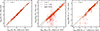 |
Fig. A.1. Comparison between the physical properties of LVL galaxies, derived using the CIGALE parameter space used in this work (introduced in Nersesian et al. 2019) and those of Dale et al. (2023). Stellar mass, dust mass and SFR are shown in the left, middle and right panel, respectively. A black-dashed line indicates the one-to-one relation. In the middle panel, a dark-red dash-dotted line shows the y= x - 0.42 relation; for 50 objects, Dale et al. (2023) only provide upper limits for Mdust, which are indicated with a different symbol. |
We would have expected significative differences also in the estimates of M* and SFR, due to the different IMF choice in Nersesian et al. (2019) and Dale et al. (2023) - which instead are not seen in Fig. A.1. Indeed, if we run our fits by assuming the Chabrier (2003) IMF (adopted by Dale et al. 2023) and leaving all other parameters unaltered, M* is found to be systematically lower than with the Salpeter (1955) IMF used by Nersesian et al. (2019), by 0.25 dex; and SFR by 0.2 dex (similar values can be found in the literature, see, e.g., Madau & Dickinson 2014; Bernardi et al. 2018). Yet, the different choice of other parameters in the two works also affects the result. In particular, we verified that the longer galactic age assumed by Dale et al. (2023, 13 Gyr vs 2-12 Gyr in Nersesian et al. 2019) conjures with the wider range in the metallicity of the stellar populations (including subsolar values, while Nersesian et al. 2019, use solar metallicity only) in raising the mass-to-light ratio of the model: eventually, the offset due to the IMF is compensated and both the Dale et al. (2023) and our fits produce similar M* and SFR.
The derivation of the physical properties of galaxies from the SED does not only depend on the selection of the parameter grid in CIGALE, but also on the wavelength coverage. For instance, Nersesian et al. (2021) shows that the shape and the wavelength of the FIR-peak of emission at ∼100 μm, correlate with dust properties, such as the dust temperature, luminosity and mass, and also with the dust-to-stellar mass ratio and the SFR. As already mentioned in Sect. 2, the galaxies in the two samples are well covered from the FUV to the FIR wavelengths. The main difference between them is that the DustPedia galaxies are observed by Herschel up to 500 μm, while the FIR data of LVL galaxies are limited to the MIPS 160 μm band. In order to check the impact of the different wavelength coverage, we took advantage of the 58 galaxies in common between the two samples, for which we have two set of CIGALE fits on a common parameter grid: those produced in this work using the LVL photometry from Dale et al. (2023); those obtained from the DustPedia photometry by Nersesian et al. (2019).
A comparison between the two CIGALE runs is shown in Fig. A.2. The change in photometric extent does not affect significantly the estimates for M* and SFR: the values obtained using the LVL photometry are close to those for the DustPedia photometry, within a small scatter (0.08 and 0.03 dex, respectively). More significant is the scatter for Mdust, a quantity directly derived from the FIR/submm photometry: the scatter between the two estimates is ≈0.4 dex, with an apparent tendency for LVL-based estimates to be lower for lower values of Mdust (see the linear fit in the middle panel of Fig. A.2). In principle, we could use this fit to correct the Mdust estimates from LVL photometry and align them with the DustPedia results: however, the sample is small and several estimates are uncertain. As an additional test, we repeated the CIGALE fits of the full DustPedia database, but limiting the photometry to data points with λ ≤ 160μm, to mimic the LVL coverage. The comparison is shown in the central panel of Fig. A.2. The fit of the two estimates is along the one-to-one line, with no significant trend. The scatter between the two different DustPedia estimates is similar to that between the estimates with LVL and DustPedia photometry for the 58 galaxies in common. Therefore, the reduced FIR-submm spectral coverage of LVL galaxies does not affect significantly the derivation of the physical properties discussed in this work, thereby allowing for the integration and joint examination of DustPedia and LVL.
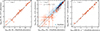 |
Fig. A.2. Comparison between the physical properties of galaxies in common between the DustPedia and LVL samples, derived from DustPedia photometry (x axis) and LVL photometry (y axis) and using the CIGALE parameter space adopted in this work. Stellar mass, dust mass and SFR are shown in the left, middle and right panel, respectively. A solid black line indicates the one-to-one relation. For both datasets we used the DustPedia distances (Clark et al. 2018). In the middle panel, the linear fit to the data is shown with a dark-red dashed line. Also, a density plot indicates the corresponding correlation for all DustPedia galaxies, where in the y axis we use the dust masses derived by restricting the photometry to the wavelength range of LVL (i.e. up to 160 μm), while in the x axis we use the results derived from the full DustPedia wavelength coverage. |
Appendix B: Correlation with morphology
The dependence of global parameters for DustPedia galaxies, such as M*, Mdust, and SFR, with morphological type is explored in Nersesian et al. (2019). In that study, the median values of the parameters, per Hubble stage bin, are computed and then fitted by a 5th order polynomial, providing the average trend of how the parameters change with morphology (see their Figs. 6, 7, and Table D.1). We apply here the same methodology to the combined sample (DustPedia+LVL) covering a wider range of stellar masses. In Fig. B.1 we plot the polynomial fits for the physical properties examined in the current work. As can be seen in the top and middle panels, M* and sMdust vary on average by two orders of magnitude across different morphologies, while the sSFR variation is ∼2.5 orders of magnitude. The maximum of the M* is for the E galaxies, with another local maximum at T ≈ 1 (Sa galaxies). In the sMdust the maximum is found at T ≈ 6 (Scd). The maximum sSFR is found for Irr galaxies, and in general LTGs with 5 ≲ T ≲ 10 have two orders of magnitude higher sSFR than earlier-type galaxies with −5 ≲ T ≲ −1. The estimated values of the coefficients of the polynomial regression of each property are provided in Table B.1. These recipes allowed us estimate the values of M*, sMdust and sSFR for a galaxy of a given Hubble stage (T). We thus use them to inspect the variation in the correlations investigated [i.e. log10(sMdust) – log10(M*/M⊙), Fig. 2; log10(sMdust) – log10(sSFR}/yr−1), Fig. 3] as a function of the morphological stage (see Sect. 4).
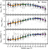 |
Fig. B.1. Variation in M*, sMdust, and sSFR as a function of Hubble stage, from top to bottom panel, respectively. In each panel grey circles correspond to individual galaxies, black squares are the median values for each morphological bin. Error bars bracket the range between the 16th and 84th percentiles from the median. The curves, colour-coded with morphology (such as the data points in Figs. 2 and 3), are the fifth-order polynomial regressions to the median values (see Table B.1 for the polynomial regression parameters). |
Recipes to estimate the integrated physical properties of galaxies given their Hubble stage (T).
The dependence of the correlations on morphology are also traced by performing linear fitting to the galaxies grouped in morphological bins. In Fig. B.2 we plot the log10(sMdust) – log10(M*/M⊙) and log10(sMdust) – log10(sSFR}/yr−1) relations, with data points colour-coded according to Hubble stage, and with the best-fit models for each morphological bin overplotted. For both investigated correlations, a dependence on the morphology is found. Scd-Sdm and Sm-Irr galaxies show a positive log10(sMdust) – log10(M*/M⊙) correlation (steeper for the latter ones), while the other four morphological bins have a negative correlation (steeper for S0s). The log10(sMdust) – log10(sSFR}/yr−1) correlation is positive for all morphological bins, with the slope getting steeper towards earlier Hubble stages (from Scd-Sdm to E); exception is the Sm-Irr bin which has a steeper relation than the Scd-Sdm galaxies.
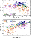 |
Fig. B.2. sMdust as a function of M* (top panel) and sSFR (bottom panel). Colour-coding is same as in right panels of Figs. 2 and 3. The best linear fits to each morphological bin is shown with the corresponding colour (see the fitting parameters in Table B.2). |
The statistics per morphological bin, along with the fitting parameters and the correlation coefficients, are listed in Table B.2. Despite some morphological types (like E) has large fractions of uncertain measures, the correlations are found to be statistically significant in all cases; following the procedures described in Sect. 5.2 of Bianchi et al. (2018), we also tested that none of them is driven by the presence of the same quantity on both axis (like, e.g., M* being used for the x axis and for the derivation of sMdust in the y axis). In both correlations, the largest dispersion is found for E galaxies (0.67 and 0.61, respectively), and the smallest for Sb-Sc galaxies (0.21 and 0.18, respectively). According to the correlation coefficients, the strongest linear and monotonic log10(sMdust) – log10(M*/M⊙) correlation is found for the ellipticals (ρP = ρS = −0.52). It is worth mentioning that if we take into account only the more certain estimates (filled circles), the correlation for Sm-Irr galaxies improves significantly (ρP = 0.61, ρS = 0.65). In the case of the log10(sMdust) – log10(sSFR}/yr−1) relation, apart from the Scd-Sdm and Sm-Irr galaxies, for the rest of the morphological bins the correlation is found to be significant and monotonic (ρP > 0.5, ρS > 0.4). Finally, it is worth pointing out that in the combined DustPedia-LVL sample, all Hubble type bins consist of a statistically significant number of galaxies.
Best-fit parameters for the correlations examined in Figs. 2 and 3, for different morphological-type bins.
Appendix C: Comparison with De Looze et al. (2020)
De Looze et al. (2020) analysed the combined JINGLE, HRS, KINGFISH, HAPLESS and H IGH sample and found an offset between their log10(sMdust)–log10(M*) relation and that of Casasola et al. (2020) for DustPedia galaxies. Since both works used the same dust model, THEMIS, the offset was attributed to a selection effect, with the dataset of De Looze et al. (2020)
including more distant (thanks to JINGLE) and dustier galaxies. The analyses of De Looze et al. (2020) and Casasola et al. (2020) also differed in the way stellar masses and SFRs were derived: while the latter used the CIGALE fits of Nersesian et al. (2019) that are also adopted in the current work, the former study by De Looze et al. (2020) derived M* and SFR using the Multi-wavelength Analysis of Galaxy Physical Properties code (MAGPHYS; da Cunha et al. 2008).
The large overlap between our datasets (DustPedia-LVL includes about half of the galaxies analysed by De Looze et al. 2020, see Sect. 2.3) should allow to investigate if the offset is due to selection effects or to different assumptions in the modelling. However, while De Looze et al. (2020) provide Mdust for the whole sample, they refer to the literature for M* and SFR; these quantities are available in a tabulated format only for KINGFISH, in Hunt et al. (2019). The comparison for KINGFISH galaxies is shown in Fig. C.1. As expected, there is no systematic offset in Mdust between our results and those of De Looze et al. (2020). Instead, our M* are found to be larger by 0.3 dex, and SFR by 0.37 dex. These systematic offsets are likely due to the differences between the CIGALE and MAGPHYS parametrisation, among which the different choice for the IMF, since MAGPHYS uses Chabrier (2003, see also Appendix A).
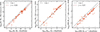 |
Fig. C.1. Comparison between the physical properties of KINGFISH galaxies as used in the analysis of De Looze et al. (2020) and those from DustPedia (this work). M*, Mdust and SFR are shown in the left, middle, and right panels, respectively. A solid black line indicates the one-to-one relation and dark-red dash-dotted lines show the systematic offsets (if any). Errors for M* and SFR for the De Looze et al. (2020) data points are not shown, because they are not available in the table they use (from Hunt et al. 2019). |
When showing the results of De Looze et al. (2020) in Figs. 2 and 3 we thus applied these offset to their quantities: 0.3 dex for M*, -0.3 dex for sMdust, and -0.07 dex for sSFR. After these corrections, the results of De Looze et al. (2020) become fully compatible with those of Casasola et al. (2020) and our work.
All Tables
Recipes to estimate the integrated physical properties of galaxies given their Hubble stage (T).
Best-fit parameters for the correlations examined in Figs. 2 and 3, for different morphological-type bins.
All Figures
|
Fig. 1. Distributions of the morphological type (top panel) and stellar mass (bottom panel) of the galaxies in our study. Blue histograms represent the distributions of DustPedia galaxies, while the pink ones correspond to the DustPedia + LVL combined sample. In the top panel the HyperLEDA parent sample, from which DustPedia was selected, is plotted with a grey histogram. Changes in the distribution, due to further selection criteria (i.e. D25 > 1′ and W1-band above 5σ) are shown with a dashed and a solid green histogram, respectively. An extra bin includes morphologically unclassified (Unc.) sources. |
| In the text | |
|
Fig. 2. sMdust as a function of M*. In the left panel DustPedia and LVL galaxies are shown in blue and pink, respectively; in the right panel galaxies are colour-coded with morphology. Objects are divided between those with larger (open and paler circles) and smaller uncertainties (filled and darker circles; see text for details): the black error bars in the left panel show the median values of the uncertainties in both ranges. In the left panel, the dashed red curve is the smoothly joined bilinear fit for LTGs, the shaded area shows the dispersion around the fit, and the two paler dashed curves indicate the fitted intrinsic scatter. We also show the fits by Casasola et al. (2020) and De Looze et al. (2020), and mark galaxies hosting AGNs or s radio jet with a ‘x’ or a ‘+’ symbol, respectively (see Sect. 3). In the right panel, the coloured curve shows the combination of the fitted fifth-order polynomials, of each physical property, parametrised with Hubble stage (from T = −5 to T = 10; pink to dark-red; see Table B.1) on the sMdust–M* plane. The uncertainty of the polynomials is indicated by the shaded grey area. |
| In the text | |
|
Fig. 3. sMdust as a function of sSFR. The colours and shapes, median error bars, and marks indicating AGNs and radio jets (left panel) are the same as in Fig. 2. In the left panel, the dashed red curve is the linear fit to LTGs with log10(M*/M⊙) > 9.5, the shaded area the 1σ dispersion around the fit, and the two paler dashed curves the fitted intrinsic scatter (the short-dashed line being the fit including also ETGs). The dotted line is the fit by De Looze et al. (2020). The black squares show the median, and standard deviation, for bins in M* of 1.0 dex width, centred from log10(M*/M⊙) = 7 (on the right side of the panel) to log10(M*/M⊙) = 12 (on the left side). In the right panel, the coloured curve shows the combination of the fitted fifth-order polynomials, of each physical property, parametrised with Hubble stage (from T = −5 to T = 10; pink to dark red; see Table B.1) on the sMdust–sSFR plane. The uncertainty of the polynomials is indicated by the shaded grey area. |
| In the text | |
|
Fig. 4. sMdust as a function of M* (left panel) and sSFR (right panel), compared to model predictions from the literature. Galaxies with uncertain estimates are shown with open symbols. Model estimates by Galliano et al. (2021, Ga21) are shown with blue squares; the lighter blue colour corresponds to a higher outflow rate (δout). The models for three spiral galaxies of different baryonic masses from Calura et al. (2009, Ca09) are plotted with green diamonds, with darker green indicating a higher assumed baryonic mass. Predictions for isolated disc galaxies by the Richings et al. (2022, Ri22) and FIRE (Choban et al. 2024, Ch24) simulations are also plotted in the left panel, with orange and yellow, respectively. In the right panel, together with the Ca09, Ga21, and Ch24 estimations, the predictions of Asano et al. (2013, As13) are also plotted with violet hexagons; lighter colours represent higher star formation timescales (τSF). Predictions by Ri22 for the right panel, and by As13 for the left panel, are not available in the literature. Galaxy age of the models is equal to 13 Gyr if not indicated. |
| In the text | |
|
Fig. 5. sMdust as a function of M* (left panels) and sSFR (right panels) compared to our model predictions using chemevol. The colour-coding of data points is the same as in Fig. 4. Model estimates are colour-coded by Mgas, init, with darker colours corresponding to older galaxies (with a larger galaxy age, tgal). Apart from Mgas, init and tgal, in each row we also vary and indicate with a different symbol (i.e. circle, square, and triangle): the cold gas fraction (fc) and the outflow reduction factor (fout; first row), the THEMIS photofragmentation rate of a-C:H/a-C grains (kfrag; second row), both kfrag and the cloud grain growth scaling factor from THEMIS (kgg, cloud; third row), and the reference SFE (fourth row). Solid black lines correspond to the isochrones. |
| In the text | |
|
Fig. A.1. Comparison between the physical properties of LVL galaxies, derived using the CIGALE parameter space used in this work (introduced in Nersesian et al. 2019) and those of Dale et al. (2023). Stellar mass, dust mass and SFR are shown in the left, middle and right panel, respectively. A black-dashed line indicates the one-to-one relation. In the middle panel, a dark-red dash-dotted line shows the y= x - 0.42 relation; for 50 objects, Dale et al. (2023) only provide upper limits for Mdust, which are indicated with a different symbol. |
| In the text | |
|
Fig. A.2. Comparison between the physical properties of galaxies in common between the DustPedia and LVL samples, derived from DustPedia photometry (x axis) and LVL photometry (y axis) and using the CIGALE parameter space adopted in this work. Stellar mass, dust mass and SFR are shown in the left, middle and right panel, respectively. A solid black line indicates the one-to-one relation. For both datasets we used the DustPedia distances (Clark et al. 2018). In the middle panel, the linear fit to the data is shown with a dark-red dashed line. Also, a density plot indicates the corresponding correlation for all DustPedia galaxies, where in the y axis we use the dust masses derived by restricting the photometry to the wavelength range of LVL (i.e. up to 160 μm), while in the x axis we use the results derived from the full DustPedia wavelength coverage. |
| In the text | |
|
Fig. B.1. Variation in M*, sMdust, and sSFR as a function of Hubble stage, from top to bottom panel, respectively. In each panel grey circles correspond to individual galaxies, black squares are the median values for each morphological bin. Error bars bracket the range between the 16th and 84th percentiles from the median. The curves, colour-coded with morphology (such as the data points in Figs. 2 and 3), are the fifth-order polynomial regressions to the median values (see Table B.1 for the polynomial regression parameters). |
| In the text | |
|
Fig. B.2. sMdust as a function of M* (top panel) and sSFR (bottom panel). Colour-coding is same as in right panels of Figs. 2 and 3. The best linear fits to each morphological bin is shown with the corresponding colour (see the fitting parameters in Table B.2). |
| In the text | |
|
Fig. C.1. Comparison between the physical properties of KINGFISH galaxies as used in the analysis of De Looze et al. (2020) and those from DustPedia (this work). M*, Mdust and SFR are shown in the left, middle, and right panels, respectively. A solid black line indicates the one-to-one relation and dark-red dash-dotted lines show the systematic offsets (if any). Errors for M* and SFR for the De Looze et al. (2020) data points are not shown, because they are not available in the table they use (from Hunt et al. 2019). |
| In the text | |
Current usage metrics show cumulative count of Article Views (full-text article views including HTML views, PDF and ePub downloads, according to the available data) and Abstracts Views on Vision4Press platform.
Data correspond to usage on the plateform after 2015. The current usage metrics is available 48-96 hours after online publication and is updated daily on week days.
Initial download of the metrics may take a while.