| Issue |
A&A
Volume 710, June 2026
|
|
|---|---|---|
| Article Number | A26 | |
| Number of page(s) | 11 | |
| Section | The Sun and the Heliosphere | |
| DOI | https://doi.org/10.1051/0004-6361/202659103 | |
| Published online | 29 May 2026 | |
Statistics of transition-region loop brightenings and their heating implication
1
Shandong Key Laboratory of Space Environment and Exploration Technology, Institute of Space Sciences, School of Space Science and Technology, Shandong University, Shandong, China
2
Institute of Science and Technology for Deep Space Exploration, Suzhou Campus, Nanjing University, Suzhou 215163, China
3
State Key Laboratory of Lunar and Planetary Sciences, Macau University of Science and Technology, Macau, China
4
Max Planck Institute for Solar System Research, Justus-von-Liebig-Weg 3, 37077 Göttingen, Germany
5
Space Research and Technology Institute, Bulgarian Academy of Sciences, Acad. G. Bonchev Str., Bl. 1, 1113 Sofia, Bulgaria
6
Korea Astronomy and Space Science Institute, 34055 Daejeon, Republic of Korea
★ Corresponding author: This email address is being protected from spambots. You need JavaScript enabled to view it.
Received:
23
January
2026
Accepted:
28
March
2026
Abstract
Context. Transition-region loops are a type of critical magnetic structure in the solar atmosphere, yet their physical properties and evolutionary characteristics remain statistically poorly constrained.
Aims. We aim to statistically characterize the physical properties of propagating brightening events in transition-region loops and to explore the underlying heating mechanism responsible for these brightenings.
Methods. Using coordinated observations from the Extreme Ultraviolet Imager on board the Solar Orbiter and the Atmospheric Imaging Assembly (AIA) on board the Solar Dynamics Observatory, we analyzed 42 propagating brightening events in loops that are unambiguously detected in both sets of instrument data. Each of these events evolves simultaneously in the AIA 94, 131, 171, 193, 211, 304, and 335 Å passband images, suggesting that they are in the transition-region or low-coronal temperature range.
Results. Our analyses show that these brightenings are impulsive, with an average brightening time of 118.4 ± 12.0 s and a mean intensity decreasing time of 159.4 ± 16.6 s. The propagating brightenings are predominantly subsonic, with velocities in the range of 0−90 km s−1 and an average of 51.3 ± 5.6 km s−1. The lengths of brightenings range from 3 to 11 Mm, with an average and standard deviation of 6.3 ± 0.4 Mm, which are closely related to the propagation velocity and the lifetime. The initial brightening sites are predominantly located near the footpoints of these loops, and the number of brightening events decreases systematically with increasing loop height.
Conclusions. Our results are consistent with an energizing mechanism regulated by enthalpy flows and radiative cooling. Dynamic magnetic evolution, including migration and cancellation, are taking place at the footpoints of these loops, and thus we suggest that magnetic cancellation, driven by reconnection and/or braiding that generate these brightenings, is a possible mechanism of plasma heating in a transition-region loop. Based on the measurements of these brightenings, we also propose a diagnostic method for the temperature or density of transition-region loops.
Key words: methods: data analysis / methods: observational / Sun: atmosphere / Sun: corona / Sun: magnetic fields / Sun: transition region
© The Authors 2026
 Open Access article, published by EDP Sciences, under the terms of the Creative Commons Attribution License (https://creativecommons.org/licenses/by/4.0), which permits unrestricted use, distribution, and reproduction in any medium, provided the original work is properly cited.
This article is published in open access under the Subscribe to Open model. This email address is being protected from spambots. You need JavaScript enabled to view it. to support open access publication.
1. Introduction
In the one-dimensional static model, the solar atmosphere is commonly described as a stratified system consisting of the photosphere, chromosphere, transition region, and corona. The photosphere is the visible solar surface; the chromosphere is the overlying layer where temperature increases gradually; and the corona is the hot outer atmosphere characterized by temperatures on the order of 1 MK and above. The transition region is the interface between the chromosphere and the corona, characterized by a rapid temperature rise over a relatively short height range. It is normally defined in the temperature regime from roughly 2 × 10⁴ K to 8 × 10⁵ K. One of the major unresolved problems in solar physics is why the temperature rises sharply from the lower atmosphere to the corona; namely, the coronal heating problem (Edlén 1940; Alfvén & Lindblad 1947; Zirker 1993; Klimchuk 2006, 2015). Loops are arcade-like features in the solar atmosphere, especially the corona, which are the results of the coupling between the solar magnetic field and the hot solar plasma. They are one of the fundamental structures of the solar atmosphere, and thus they are ideal objects to study and with which to resolve the coronal heating problem (Del Zanna & Mason 2003; Reale 2014; Huang et al. 2015; Fletcher et al. 2015). Based on the temperature, loops are usually classified as cool (< 1 MK), warm (1−2 MK), and hot loops (> 2 MK) (Reale 2014). In terms of heating timescales, heating is commonly divided into impulsive heating and steady heating. Independent heating events with heating times shorter than the cooling times are regarded as impulsive heating (Cargill & Klimchuk 2004; Warren et al. 2011), whereas heating with timescales much longer than the cooling times, or the case in which numerous impulsive events occur in rapid succession (Lu et al. 2024), is treated as steady heating (Li et al. 2015). The density and magnetic field strength of coronal loops usually decrease with height along the loop (Gary 2001; Xie et al. 2017). The electron density in loops at coronal temperatures is generally on the order of 109 cm−3 or lower (Reale 2002; Aschwanden et al. 2008; Huang 2018).
The heating distribution along loops, i.e., the location of energy deposition, provides a key constraint for establishing the heating mechanism(s) at work. Numerical modeling shows that, for different choices of heating duration, power, and frequency, footpoint heating, approximately uniform heating, or apex heating, can reproduce various observed properties (Priest et al. 2000; Aschwanden et al. 2000, 2001; Aschwanden 2001; Reale 2002; Warren et al. 2011). High-resolution observations further reveal that mixed polarity magnetic field and their activity, for example cancellation, near loop footpoints likely play a key role in heating the plasma to transition-region and coronal temperatures, and that the actual heating often exhibits multistranded, intermittent, and highly nonuniform spatial characteristics (Chitta et al. 2017, 2018; Huang et al. 2019b).
In addition to long and high coronal loops, active regions are also populated by numerous short, low-lying loops, many of which are in the transition-region to low-coronal temperature range. Here we refer these loops with transition-region temperatures as transition-region loops. Transition-region loops normally have a compact morphology, rapid evolution, and multi-thermal EUV response, and these are consistent with relatively cool plasma rather than hot coronal loops (Huang et al. 2015). The density, temperature, and dynamical properties of transition-region loops differ significantly from those of coronal loops. Because of the scarcity of suitable observations, transition-region loops have not been well studied. Since the advent of Interface Region Imaging Spectrograph (IRIS, De Pontieu et al. 2014), a number of studies have investigated the physical parameters of transition-region loops. The IRIS Si IV 1400 Å slit-jaw images and spectra directly resolve numerous, highly dynamic, low-lying transition-region loops (Hansteen et al. 2014; Pereira et al. 2018). These loops typically have lengths of only a few megameters, heights of about 1−4 Mm, lifetimes of several minutes, and evolution timescales of tens of seconds to a few hundred seconds (Hansteen et al. 2014; Pereira et al. 2018; Dolliou et al. 2025). Many studies showed that transition-region loops have peak temperatures generally below 0.5 MK, while their densities can reach 1011 cm−3 or even higher, significantly higher than those of coronal loops (Kjeldseth-Moe & Brekke 1998; Huang et al. 2015; Liang et al. 2024). Hansteen et al. (2014) pointed out that such structures can be driven by intermittent heating associated with magnetic braiding.
Transition-region loops are highly dynamic (Kjeldseth-Moe & Brekke 1998), and are possibly accompanied by a variety of small-scale energy release processes, and their dynamics plays a crucial role in the transport of mass and energy between the chromosphere and corona (Huang et al. 2017, 2019a). Early spectroscopic studies already revealed flows, oscillations, and explosive events (EEs) in the transition region (Dere et al. 1989; Kjeldseth-Moe & Brekke 1998; Brynildsen et al. 1999). Using IRIS data, Huang et al. (2015) found siphon flows in some cool transition-region loops, with Doppler velocities varying continuously along the loop from about 10 km s−1 at one footpoint to about 20 km s−1 at the other. Many studies based on IRIS data showed that many transition-region loops are closely associated with small-scale activities such as EEs and ultraviolet (UV) bursts (e.g., Huang et al. 2015, 2019a; Hou et al. 2021, and references therein). Other studies indicate that the dynamics of transition-region loops can lead to small-scale brightenings in moss regions (Ram et al. 2024), where propagating bright fronts along the loops are clearly visible, with an apparent velocity on the order of tens of km s−1 (Hou et al. 2021). Simulations of transition-region loops suggest that reproducing the observed IRIS signatures requires highly intermittent heating in time (multiple, high-frequency events), multi-scale heating, and strongly nonequilibrium ionization (Bahauddin & Bradshaw 2024). Magnetohydrodynamic simulations show that random motions of magnetic footpoints in a bipolar system can generate numerous small-scale loops heated to transition-region temperature, whose lifetimes and kinematics are comparable to the observation events (Skan et al. 2023). More details about magnetic loops in the solar transition region are referred to a recent review (Huang 2026).
Current studies of activities in transition-region loops, however, focus on individual events, such as EEs and UV bursts. Systematic constraints on the statistical properties of brightenings in transition-region loops in active regions, such as the length of the brightening segment (Lb), their propagation velocity along the loops, and heating and cooling times, remain scarce. Our statistical analysis is based primarily on the high spatial and temporal resolution data from the Extreme Ultraviolet Imager (EUI, Rochus et al. 2020) in the 174 Å passband. We investigate 42 brightening events (internal fine-scale activity) in transition-region loops. We compile the relevant physical parameters describing their dynamics, including brightening durations, Lb, and the propagation velocity of brightening fronts, and based on the magnetic field evolution in this region, we suggest possible physical mechanisms responsible for these brightening events. These results are of significant value for current coronal heating studies, especially for understanding the heating mechanisms of transition-region loops, and provide key constraints for future related studies. The remainder of this paper is organized as follows. Section 2 presents the observations. Section 3 describes the data analysis and results. Section 4 provides the discussion. Section 5 summarizes our conclusions.
2. Observations
In this study, we utilized observations from the Atmospheric Imaging Assembly (AIA, Lemen et al. 2012) and the Helioseismic and Magnetic Imager (HMI, Scherrer et al. 2012) on board the Solar Dynamics Observatory (SDO, Pesnell et al. 2012), and the EUI/Solar Orbiter (SO, Müller et al. 2020). The EUI instrument consists of three telescopes: the Full Sun Imager (FSI), which operates at 174 and 304 Å passbands, and two High Resolution Imagers, namely HRIEUV and HRILyα. The FSI 174 Å passband provides full-disk EUV images that are used to locate the region of interest (ROI) on the solar disk (Fig. 1b) and the HRIEUV provides high-resolution data for detailed loop structure analysis (Fig. 1c). The observations analyzed here were obtained from the EUI Data Release 6.0 (Kraaikamp et al. 2023), and they are a part of the Solar Orbiter Observing Plan (SOOP) named “R_BOTH_HRES_HCAD_Nanoflares”. The data were acquired on April 11, 2023, and focused on the peripheral portion of active region AR 13269. During these observations, SO was located at a heliocentric distance of 0.29 AU. The SO–SDO observing times differ by 360 s, reflecting the light-travel-time offset. The longitudinal separation angle between the two lines of sight is 68° (Fig. 1a), and the solar latitude of SO was 2.26°. In the EUI field of view, the ROI lies slightly to the east of the disk center, whereas in the AIA field of view was slightly to the west of the disk center. This longitudinal separation allows us to view the brightenings from different angles and to reduce the impact of projection effects that may otherwise obscure the structures. The co-alignment between the SO and SDO data was determined from the relative observing angle of the two instruments and refined through visual comparison of common structures in the ROI, including bright dots, loop footpoints, and intersections (Zuo et al. 2025).
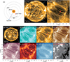 |
Fig. 1. Overview of the study. Panel (a) shows the observation positions of SDO and SO. Panel (b) presents the full disk of the Sun in EUI 174 Å passband, of which the purple box indicates the ROI location in the HRI field of view, situated near the equatorial region on the left side of the solar surface. Panel (c) is the ROI in a high-resolution image of the HRIEUV passband. Panel (d) shows the full disk of the Sun in AIA 171 Å passband, of which the blue box marks the ROI position in the AIA field of view, located near the equatorial region on the right side of the solar surface. Panels (e)–(j) display the ROI images of AIA passbands, where multiple distinct loops connect the magnetic polarity regions in the upper left and lower right. Panel (k) shows the HMI magnetic field image of the ROI scaled from −300 G (black) to 300 G (white), with the primary positive polarity region in the upper left field of view, the main negative polarity region in the lower right, and numerous small-scale polarity points distributed in the central region. |
The time interval of interest for HRI observations is 21:34–23:34 UT. The HRI data have a spatial resolution of 0.492″, corresponding to a pixel size of about 110 km, and a temporal cadence of 3 s and 5 s. The AIA/SDO provides data with a temporal resolution of 12 s and a spatial resolution of 426 km pixel−1. In the HRIEUV images, the loops are clearly identifiable (Fig. 1c). For the events analyzed in this study, the observed loops are identified based on their coherent, continuous, arc-shaped morphology in the HRIEUV images. Their widths are generally larger than 5 pixels (about 550 km), whereas their projected lengths typically range from several tens to a few hundred pixels. The measured loop widths are significantly larger than the point spread function (PSF) scale that is about 220 km (Chitta et al. 2022). These characteristic sizes, together with the clear loop-like continuity, support the identification and tracking of the observed structures as loops. This enables us to analyze parameters such as the loop length, Lb (length of brightening segment), propagation velocity, brightening time, and intensity decreasing time. Nevertheless, finer strand-like substructure, if present, may remain unresolved in the current data and will require future observations with a higher spatial resolution.
The HRIEUV passband is most sensitive to plasma with temperatures around 1 MK. Because of its relatively broad temperature response, plasma at several 105 K also strongly contributes to this passband, providing the physical basis for using these data to study transition-region loops. AIA supplies observations in seven EUV passbands (94, 131, 171, 193, 211, 304, and 335 Å passbands). Although its lower spatial and temporal resolution prevents us from resolving the fine loop morphology in the AIA field of view, these passbands together cover emission lines formed over a wide temperature range from several ×104 K to several ×107 K, which is highly advantageous for our temperature estimation. The HMI data have a spatial resolution of 0.6″ per pixel and a temporal cadence of 45 s, and we used the HMI data to investigate the magnetic field evolution of the active region (Fig. 1f), which allowed us to analyze the evolution of the magnetic field at the loop footpoint.
3. Data analysis and results
Figure 1 presents the overview of the ROI. The SDO and SO viewed the ROI from different vantage angles (Fig. 1a), and the ROI appears nearly symmetrically located within the fields of view of the two instruments, which helps mitigate projection effects associated with viewing geometry (Figs. 1b and d). As is shown in Figs. 1c–j, owing to the differing perspectives, most loops appear as upward convex arches in the HRI field of view, whereas they appear with an opposite curvature in the AIA view. These loops primarily connect the dominant positive polarity region in the upper left and the dominant negative polarity region in the lower right, while a subset of shorter loops connect within the intermediate zone. To enable uniform quantitative measurements of loop brightening events, we co-aligned the HRIEUV data with the AIA data in both time and space (Fig. 1). Brightening events were then identified and marked by visual inspection, and time-slice (T–S) analysis along the loop trajectories in the HRIEUV field of view was used to extract light curves and to quantify event properties. Following this procedure, we identified 202 brightenings in the HRI data, among which 42 events can be clearly recognized in the AIA field of view and satisfy the requirements for subsequent quantitative analysis (i.e., the loop is unambiguously resolved, the brightening evolution is fully covered in time, and the morphology is not severely affected by complex loop superposition due to projection effect). We therefore performed our statistical measurements on these 42 events (see Table A.1).
For each event, we defined a sampling path along the loop and obtained the intensity distribution along the loop for each frame. This allowed us to construct a two-dimensional T–S map that characterizes the evolution of a brightening along the loop with time (Fig. 2). The T–S maps were used for the following purposes: to extract light curves and measure timescales; to determine the apparent propagation velocity of the brightening front along the loop (Fig. 2b); and to analyze the initial brightening location. The HRIEUV data used here have cadences of 3 s and 5 s. Out of 42 events, 37 were observed at 5 s cadence and 5 events at 3 s cadence (see Table A.1). For the timescale measurements, we extracted light curves from a temporal window extending approximately one minute before and after each event (about 10 frames for the 5 s cadence data and about 20 frames for the 3 s cadence data), so that the event was located near the center of the analyzed time interval. The light curves were obtained by integrating the intensity along the selected loop path. For a few events, however, the temporal window was slightly adjusted because neighboring brightenings affected the pre-event or post-event background. As a result, the number of frames selected before and after the event was not always identical. This interval includes a representative background level for subsequent quantification. We defined the event background intensity “mean” as the average of the lowest 50% of intensity samples within this interval. The start time was defined as the first time the intensity exceeds mean + 0.1*(max−mean), where “max” is the maximum intensity in the interval. The brightening phase ends when the intensity reaches its peak, after which the event enters the intensity decreasing phase. The intensity decreasing phase ends when the intensity decreases back to mean + 0.1*(max−mean) (Fig. 2c). Figure 2d shows the response curves of the HRI and the AIA passbands. The AIA passbands generally exhibit highly similar temporal evolution, with nearly co-temporal peaks. The vast majority of the 42 events exhibit this behavior, providing a critical observational constraint for determining loop-temperature characteristics (Section 4).
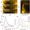 |
Fig. 2. Case-analysis methodology. Panel (a) shows the evolution of Case-13. The dashed green line marks the trajectory of the brightening loop. Panel (b) presents the T–S map, constructed along the dashed green trajectory in panel a3; the solid white line indicates the propagation velocity of the brightening front. The T–S map was used to derive the characteristic timescale, Lb, propagation velocity, and other physical properties of the event. Panel (c) shows the schematic illustration of the timescale determination based on the light curve obtained by integrating the intensity along the selected loop path. The dashed blue line denotes the mean intensity of the lowest 50% of pixels, and the dashed red lines indicate the reference baseline used to identify the brightening and intensity decreasing phases. Panel (d) displays the light curves from multiple AIA passbands and the HRIEUV passband. |
Figures 3a–c summarize the timescale statistics of the 42 events derived from the above definitions. The results indicate an impulsive character: brightening and intensity decreasing times show similar distributions, with most events falling within 20−160 s, and the highest occurrence is in the 60−80 s bin. A small number of events exhibit brightening and intensity decreasing times exceeding 300 s. The mean brightening time is 118.4 ± 12.0 s, and the mean intensity decreasing time is 159.4 ± 16.6 s (i.e., the latter is 1.35 times larger). The total duration is primarily distributed between 40 and 400 s, with a mean of 277.7 ± 20.5 s. We note that the measured brightening time may exceed the true heating timescale. After energy input ceases, a finite time is required for energy and mass transport to reach the maximum observable brightening extent. Consequently, the true cooling-to-heating time ratio may exceed 1.35.
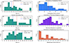 |
Fig. 3. Statistical properties of 42 brightening events. Panels (a)–(c) show the distributions of the brightening time, intensity decreasing time, and total duration. The dashed red lines mark the mean values and the dashed blue lines mark the medians. Panel (d) shows the distribution of the propagation velocities of the brightening fronts. The dashed red and green lines denote the mean and median, respectively. Panel (e) displays the distribution of the maximum Lb, defined as the length of the contiguous brightened segment along the loop at the time of peak brightening. The dashed red and blue lines indicate the mean and median. Panel (f) presents the distribution of the initial brightening location, defined as the distance between the first clearly visible bright structure and the footpoint, normalized by the loop length. The detailed parameters of each event are listed in Table A.1. |
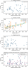 |
Fig. 4. Two-dimensional correlation analysis. Panel (a) shows the correlation of Lb and the footpoint distance. Panel (b) displays the correlation of Lb and the propagation velocity. The solid green line was obtained from grouped mean data by linear fitting. Panel (c) presents the correlation of Lb and the brightening time. Panel (d) presents the correlation of the brightening and intensity decreasing time and footpoint distance. The pink dots represent the brightening time and the blue dots represent the intensity decreasing time. |
Figure 3d presents the apparent propagation velocities along the loop derived from the T–S maps. For each event, we tracked the main boundary of the brightening front in the T–S map and defined the propagation velocity as v = Δs/Δt, where Δs is the propagation along the loop over a time interval, Δt. The majority of events exhibit subsonic velocities in the range of 0−90 km s−1, with the 0−15 km s−1 bin being the most populated. The mean velocity is 51.3 ± 5.6 km s−1, and the median is 38.4 km s−1. There are seven events that yield v ≈ 0, indicating that the brightenings remain stationary at their initial sites without significant propagation along the loop.
Figure 3e shows the distribution of Lb. To quantify the spatial “impact range” of a single event, we defined the maximum Lb as the length of the contiguous enhanced intensity segment along the loop at the time of the strongest brightening. In practice, we applied a threshold to the along-loop intensity profile for the frame in which the bright segment is most prominent. Pixels exceeding the threshold were classified as brightening, and the length of the contiguous above-threshold segment was converted to a physical length. For a subset of events, strong loop superposition or an exceptionally bright background near the footpoints prevents robust application of this threshold. In these cases, we adopted a different method: we selected a pre-event frame where the loop is uniformly faint, subtracted it from the brightest frame to obtain an intensity enhancement map, and estimated the brightened length from this map. The results show that most events have Lb in the range of 3−11 Mm, with the highest frequency in the 5−8 Mm bin. The mean Lb is 6.3 ± 0.4 Mm, and the median is 5.8 Mm. Given the viewing geometry and projection effects, these lengths likely represent lower limits to the true values. For a few events, the brightening segment reached the footpoints (Nos. 17, 25, and 33). These events have brightening ratios exceeding 0.9 (see Table. A.1), meaning that the entire loop became bright. In these cases, the brightening length may have been limited by the loop length. We further note that bright footpoint backgrounds (e.g., a moss region) and multi-loop superposition introduce systematic uncertainty in the identification of bright segment boundaries. This uncertainty should be treated as a non-negligible error source when interpreting the length distribution and derived correlations.
Figure 3f summarizes the statistics of initial brightening locations. We define the initial brightening point as the location where a clear bright structure is first observed, quantified by the ratio of the distance from the footpoint to the initial brightening site relative to the loop length (L). The results show a pronounced footpoint preference: events are concentrated within 0−0.25 L, and the occurrence decreases monotonically with height within 0−0.5 L (Fig. 3f). This implies that, at least observationally, energy deposition and/or the first detectable brightening preferentially occur at low heights near the footpoint. Based on representative examples (Figs. 5 and 6), we further categorize the events into four morphological classes: (I) Four cases in which a brightening starts near a footpoint with no obvious loop-loop interaction; one example is shown in Figs. 5a1–a8. (II) Sixteen cases in which a brightening is footpoint triggered but shows migration of bright kernels adjacent to the footpoint or brightening of small loops (Figs. 5b1–b8). (III) Twenty cases in which a brightening occurs along the loop, often accompanied by vigorous evolution of multiple intersecting or entangled small-scale loops (e.g., loop approach, loop separation, and along-loop propagation of bright segments (Figs. 6a1–a8). (IV) Two cases of brightening with bidirectional jets consistent with reconnection outflows (Figs. 6b1–b8).
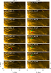 |
Fig. 5. Evolution detail of brightening events. Panels (a1)–(a8) present the brightening process of Case-3; the event brightens at a footpoint, and the brightening front propagates along the loop over a finite distance. Panels (b1)–(b8) show the brightening process of Case-6; the event also brightens from the footpoint. As is indicated by the green arrows, small, moving, brightening points are observed near the footpoint, which may provide evidence of reconnection between shorter and longer loops. |
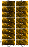 |
Fig. 6. Evolution detail of brightening events. Panels (a1)–(a8) present the brightening process of Case-21, the event brightens near the loop apex, with multiple loops intersecting and separating during the evolution. Panels (b1)–(b8) show the brightening process of Case-41, as is indicated by the red arrows, bidirectional jet-like features are observed during the brightening process, which may represent key observational signatures of magnetic reconnection between loops. |
Based on the statistical results shown in Fig. 3, we further analyzed the correlations among these physical properties and examined their two-dimensional relationships in the parameter space (Fig. 4). To reduce the influence of scatter and emphasize overall behavior, we sorted the independent variable and grouped the sample into bins of five events (Fig. 4b). For each bin, we calculated the mean and standard deviation and plot error bars. For pairs showing an apparent linear trend, we fit a linear regression to the binned means and report the corresponding correlation coefficient. The key results include: In panel a, the scatter between Lb and footpoint distance is large with no clear systematic trend, indicating a weak overall correlation. This suggests that the spatial extent of a single brightening does not scale linearly with the loop’s geometric size. In panel b, a clear positive trend exists between Lb and propagation velocity, i.e., faster events tend to produce longer brightening segments. In panel c, Lb shows no significant correlation with heating time, implying that the duration of energy release and the resulting observable Lb can be statistically decoupled. In panel d, neither the brightening time nor the intensity decreasing time shows a clear correlation with the footpoint distance.
4. Discussion
The timescale statistics quantify the above thermal-response constraints into limits that can be directly used for physical inference. The characteristic times of the brightening and intensity decreasing phases are generally on the order of 100 s (< 300 s), with the intensity decreasing phase systematically longer than the brightening phase (mean brightening time tb = 118.4 ± 12.0 s, mean intensity decreasing time td = 159.4 ± 16.6 s, and td/tb ≈ 1.35). Together with the highly synchronous responses across the AIA passbands, this “short impulse plus slightly trailing decay” pattern suggests a rapid-cooling scenario under transition-region or low-coronal conditions. To assess the relevant cooling mechanisms, we compared the observed timescales with conductive and radiative cooling estimates. The conductive cooling times can be written as
 (1)
(1)
where n is the particle density at the end of the heat pulse, kB is the Boltzmann constant, T is the plasma temperature, L is the loop length, and κ is the thermal conductivity (Reale 2014). For representative parameters of our events, we adopted L = 15 Mm, n = 1010 cm−3, κ = 9 × 10⁻⁷ erg s−1 cm−1 K−7/2, and T = 0.4 MK, which gives τc ≈ 3.5 × 10⁵ s. This value is far longer than the observed intensity decreasing timescale (with an order of 100 s), indicating that classical conductive cooling is unlikely to be the dominant mechanism controlling the rapid intensity decreasing of these events. By contrast, the radiative cooling times can be written as
 (2)
(2)
where n is the plasma density and Λ(T) is the optically thin radiative loss function (Cargill & Klimchuk 1997, 2004; Winebarger et al. 2013; Reale 2014). For T = 0.4 MK, n = 1010 cm−3, and Λ(T) = 8.87 × 10⁻¹⁷T−1 (Klimchuk et al. 2008), we obtained τR ≈ 80 s, which is close to the observed intensity decreasing timescale. The rapid intensity decreasing is therefore more consistent with radiative cooling than with classical conductive cooling. In a relatively high-density environment, the redistribution of energy and mass along the magnetic field, such as enthalpy-flux regulation, may still act together with radiation to shape the decay phase, yielding a statistical preference for td ≳ tb. More importantly, these timescales provide an order-of-magnitude constraint on the “visibility time interval”: the effective duration, τ, over which the brightened structure maintains an identifiable contrast above the background is unlikely to be much larger than 100 s; otherwise, a substantially longer duration distribution would be expected. We therefore took τ ≈ 100 s as a key premise for subsequent interpretations of spatial extension and correlations.
The velocity statistics provide dynamical constraints on “field-aligned responses or transport”, but their physical meaning should be interpreted with caution. The apparent propagation velocities of the intensity front are mainly distributed in the range of 0−90 km s−1 (mean = 51.3 ± 5.6 km s−1, median = 38.4 km s−1). For a characteristic plasma temperature of 0.4 MK, the adiabatic sound speed is
 (3)
(3)
where γ is the adiabatic index, kB is the Boltzmann constant, T is the plasma temperature, μ is the mean molecular weight, and mp is the proton mass (Kolotkov et al. 2019). Assuming a fully ionized plasma, we adopted γ = 5/3 and μ = 0.6, yielding cs ≈ 100 km s−1. Most of the measured apparent propagation velocities are therefore below the local sound speed. Because these velocities are inferred from the apparent displacement of the intensity front in T–S maps, they may trace the front of a thermal disturbance, a pressure-gradient-driven field-aligned response (including density enhancements regulated by enthalpy flux that can brighten multiple passbands nearly simultaneously), or an apparent propagation produced by sequential energization of multiple unresolved strands. The coexistence of subsonic velocities and v ≈ 0 events favors a relatively gentle field-aligned response or transport, rather than strong shock-like high-velocity propagation as a ubiquitous scenario; meanwhile, the near-zero-velocity events suggest that not all brightenings require substantial field-aligned extension, and that localized energy deposition followed by predominantly local radiation and decay can also produce the observed evolution.
Against the backdrop of an effective time interval of τ ≈ 100 s and subsonic field-aligned responses, the two-parameter relationships provide key evidence linking timescales, velocities, and spatial extension. We find that the visible brightened segment in a single event is typically only a few millimeters in length (concentrated in 3−11 Mm, with mean = 6.3 ± 0.4 Mm). The overall correlations of Lb with the geometric scale of the loop (footpoint distance) and with the brightening timescale are weak, whereas a clearer positive trend is found with the propagation velocity (v). This suggests that the energy deposition relevant to the observable brightening is confined to a relatively limited spatial extent and is not strongly tied to the loop length, and that the transport of the brightening front plays a dominant role in setting Lb. These properties provide a plausible criterion for interpreting the energy transport in terms of enthalpy flux, i.e., energy carried along the field lines by enthalpy flux; given the high-density transition-region environment, radiative cooling is then expected to be important as well. Such apparent propagation may also reflect motion of the heating location; for example, Zuo et al. (2025) report an observational case in which the unbraiding sites (heating location) migrated along the braiding axis at ∼45 km s−1, consistent with a heating scenario involving multiple interacting loops.
The onset locations of the brightenings show a statistically significant preference for the footpoints, with a peak at 0−0.25 L and a monotonic decrease with height. Based on the fine-scale properties at the heating site, the events can be grouped into four categories: (I) four events that start at the footpoints without obvious inter-loop interactions; (II) sixteen events that are footpoint-triggered and that exhibit migrating brightenings, which may reflect reconnection between a long loop and shorter loops rooted in the legs, where reconnection heats the plasma (producing the observed brightening) and the post-reconnection structures subsequently move under magnetic tension, leading to the apparent migration; (III) twenty events that brighten along the loop and shows braided, multi-loop evolution, in which crossing structures may undergo a sequence of reconnection episodes, and the moving post-reconnection loops can again satisfy reconnection-favorable geometries with other loops (Mondal et al. 2026); and (IV) two events that show along-loop brightenings accompanied by bidirectional jets, which constitutes one of the key observational signatures of magnetic reconnection. These results establish an observationally grounded “heating location” constraint: for our sample, the earliest visible energy deposition or radiative enhancement preferentially occurs near the footpoints, rather than at the apex or at random locations along the loop. We emphasize that this “footpoint preference” is not driven by a few case studies but holds for the full sample under a uniform event definition and measurement procedure, and thus should be regarded as a basic constraint that viable mechanisms must satisfy. This is broadly consistent with the conclusions of Aschwanden et al. (2001), who showed that extending uniformly heated models into the transition region can lead to unrealistic results (e.g., an excessively thick transition-region layer and column depths far exceeding observations), whereas footpoint-heating models with a scale height of ∼13 Mm can better reproduce the observed temperature distribution and flux profiles. More generally, coronal loop heating models spanning footpoint heating, apex heating, multi-site heating, and quasi-uniform heating can each reproduce certain observational signatures (Aschwanden et al. 2001; Reale 2002; Chitta et al. 2020), suggesting that the heating location in coronal loops may not exhibit a universal preference.
Compared with typical coronal loops at T > 1 MK, the TR loop brightenings studied here evolve on shorter timescales. In these loops, both brightening and intensity decreasing generally occur within about 100 s (< 300 s). This difference should not be attributed to loop length alone. In general, cooling timescales can depend on loop length when conductive cooling is important. For the representative parameters of our events, however, the classical conductive cooling timescale is much longer than the observed intensity decreasing timescale, whereas the radiative cooling timescale is much closer to the observations. This suggests that thermal conduction is unlikely to dominate the cooling of these TR loop brightenings, and that their rapid intensity decreasing is more likely governed primarily by radiative cooling under relatively cool and dense plasma conditions. In this sense, the cooling evolution in our sample is expected to be less sensitive to loop length. For hotter coronal loops, thermal conduction is often expected to play an important role during the early stage of the cooling evolution after the heating phase ends (Reale 2014). Thus, the early cooling behavior of such coronal loops is generally more closely related to loop length than that of the events studied here.
By contrast, coronal loop studies commonly find heating phases lasting from minutes to tens of minutes, followed by cooling over tens of minutes to hours and producing systematic, temperature-dependent delays across multiple passbands (Reale 2014; Li et al. 2015). The review by Reale (2014) further noted that hot active-region coronal loops are likely highly multistranded and may be continuously energized by heating events (nanoflares), rather than undergoing a single heating episode followed by free cooling. Such repeated small-scale energy injections can maintain high temperatures and emission measures on average; even if individual strand cools rapidly, the out-of-phase superposition can yield a long-duration radiative evolution at macroscopic scales (Ugarte-Urra & Warren 2014; Lu et al. 2024). In addition, the temperature dependence of the radiative loss function should also be taken into account. Around and below about 0.5 MK, the radiative loss function rises rapidly (Klimchuk et al. 2008), which favors faster radiative cooling, whereas at higher temperatures its variation becomes shallower, leading to a longer radiative cooling timescale. Therefore, the longer cooling timescales commonly observed in hotter coronal loops likely reflect not only multistranded or repeatedly heated conditions, but also the intrinsic temperature dependence of the radiative loss function. A multistranded interpretation cannot be excluded for the TR loops studied here. In our statistical results, the apparent brightening sites are often concentrated near the footpoints (Fig. 3f). If an observed loop actually consists of multiple unresolved strands, then these strands would need to be located very close to one another, with intersections or heating sites clustered within a small spatial range and triggered nearly simultaneously, so that the resulting emission still appears as a single impulsive brightening. Under the current instrumental resolution, such a scenario would observationally be expected to show a coherent loop-like morphology, a compact, localized brightening onset, and little clearly separable transverse substructure. Higher-resolution observations will be needed to determine whether such fine substructure is present in this kind of transition-region loops.
Consistent with these timescale differences, intensity disturbances or thermal front propagation in coronal loops are often tens of km s−1 to ∼100+ km s−1, comparable to slow-mode wave velocities or thermal-front velocities in ∼1 MK plasma (Reale 2014), whereas the apparent propagation in TR loop brightenings more frequently lies in a subsonic and comparatively low-velocity regime. Overall, this contrast – between TR loops of seconds to minutes and low velocities, and coronal loops of minutes to hours and higher velocities – suggests different heating and transport regimes. This difference is less likely to be mainly controlled by loop length, as neither the brightening time nor the intensity decreasing time shows a clear correlation with the footpoint distance (Fig. 4d). In this sense, TR loops may be more consistent with a single or brief impulsive response, whereas coronal loops more likely reflect multiple heating impulses and prolonged cooling. At the same time, however, we cannot exclude the possibility that some TR loop brightenings involve multiple impulsive heating episodes in multiple strands, as was discussed above.
We interpret the energy and mass-transport mechanism in these brightenings in terms of enthalpy flux, i.e., a field-aligned mass flow with finite velocity that transports energy along the loop as the plasma cools. The enthalpy flux mechanism provides an alternative diagnostic approach for transition-region plasma. In this framework, the energy transported by a field-aligned mass flow is assumed to be radiated away locally, leading to an energy balance condition: Fh ≈ n2Λ(T)l. The enthalpy flux is given by  , with p = ηnkBT and η ≈ 2, which yields Fh = 5nkBTv. Rearranging the energy balance yields a diagnostic expression:
 (4)
(4)
where n is the density, l is the length of the brightening segment, v is the flow velocity, and Λ(T) is the radiative loss function (Raymond & Doyle 1981; Klimchuk et al. 2008).
If we adopt Λ(T) = 8.87 × 10⁻¹⁷ T−1 for 104.97 < T ≤ 105.67 K (Klimchuk et al. 2008), take kB as the Boltzmann constant, assume a typical transition-region or low-coronal density n = 1010 cm−3, use the median brightening length lm = 6.3 Mm, and the median propagation velocity vm = 38.4 km s−1, we obtain T ≈ 0.46 MK. This temperature estimate is consistent with the typical transition-region temperature range and well matched to the response profiles of the AIA passbands (Fig. 2d). Furthermore, if the temperature is known, this method can be readily extended to perform plasma density diagnostics. We note that the results presented here are only rough estimates, and thus should be interpreted with caution. This is because a precise calculation for any particular loop cannot be achieved with the current dataset, owing to substantial diversity in plasma density and the radiation loss function. That said, this method proposes a novel approach to temperature and density diagnostics in the transition region and low corona that merits further investigation and in-depth validation in future studies.
The HMI magnetic field data provide evidence of field evolution consistent with footpoint-driven intermittent energy release, although the limitations in temporal and spatial resolution prevent a strict one-to-one correspondence between individual events and specific magnetic features. Figures 7a1–h1 show magnetograms of the primary source region over 21:30:45–24:00:00 UT (about 2.5 h), and Figs. 7a2–h2 further overlay ±50 G contours to highlight the evolution of the magnetic structure. The contour morphology changes markedly over time and is accompanied by patch motions, coalescence, and fragmentation, as well as local emergence and cancellation, indicating ongoing flux redistribution and topological restructuring during the observing time. Correspondingly, Figs. 7i–k show the flux evolution within the region in Fig. 7a1: the total flux changes from −2.8 × 10²⁰ Mx to −2.2 × 10²⁰ Mx; the positive flux increases from 5.1 × 10²⁰ Mx to 5.5 × 10²⁰ Mx; and the negative flux evolves from −8.0 × 10²⁰ Mx to −7.6 × 10²⁰ Mx. Notably, multiple short-lived peaks are superposed on the overall trends, implying that the flux evolution is not smoothly monotonic but rather composed of intermittent small-scale variations that phenomenologically echo the impulsive nature of the brightenings. The evolving contours and the multi-peaked flux curves suggest that processes such as flux cancellation and magnetic braiding may have operated during this interval, providing necessary conditions for magnetic energy release. Nevertheless, we emphasize that this inference should be treated with caution, because the complexity of the field evolution, together with HMI’s spatial resolution and projection effects, makes it difficult to establish a strict one-to-one association between a given brightening and a specific cancellation and coalescence episode.
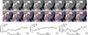 |
Fig. 7. Magnetic field evolution. Panels (a1)–(h1) present the HMI magnetograms of the main region, where the brightening events occur. Panels (a2)–(h2) are the same as panel a, but overlaid with ±50 G magnetic field contours, facilitating the identification of magnetic polarity motion, emergence, and cancellation. Red and blue contours represent positive and negative magnetic polarities, respectively. Panels (i)–(k) show the temporal evolution of the total magnetic flux, positive magnetic flux, and negative magnetic flux of the region in panel a1. |
5. Summary
Based on coordinated observations from EUI/SO and AIA/SDO, we present a statistical investigation of transient brightening events occurring in transition-region loops. Taking advantage of the dual-viewpoint observing geometry and a unified T–S analysis, we identify 42 events for statistical analysis. After correcting for instrumental time lag, the light curves of all AIA EUV passbands exhibit highly simultaneous temporal evolution: the brightening and subsequent intensity decreasing occur nearly simultaneously, with well-aligned peak times across passbands. The observations are consistent with impulsive plasma responses in the transition-region to low-coronal temperature range, where the radiative enhancement is primarily modulated by density variations. Statistical analyses of the characteristic timescales further reinforce this interpretation. The events display clear impulsive signatures, with a mean brightening time of 118.4 ± 12.0 s and a mean intensity decreasing time of 159.4 ± 16.6 s. Such temporal asymmetry favors rapid cooling influenced by radiative losses and field-aligned enthalpy flux regulation.
The apparent propagation velocity of the intensity fronts predominantly lies within the subsonic range of 0−90 km s−1, with an average value of 51.3 ± 5.6 km s−1, while the visible Lb in individual events is typically limited to only a few megameters (3−11 Mm). The Lb shows only a weak dependence on the geometric loop length, but exhibits a clearer correlation with the propagation velocity. This behavior is consistent with a scenario in which field-aligned transport within a limited effective time interval governs the spatial extent of the brightening, i.e., Lb ∼ vτ, where τ is constrained by a rapid cooling process on the order of 100 s. Based on the enthalpy-flux mechanism and key parameters (e.g., vm and lm) of brightening events, we propose a potential diagnostic method for the temperature and density of the transition region. The temperature derived from this method is consistent with the typical temperature characteristics of the transition region and also matches the response profiles of AIA passbands. The initiation sites of the brightenings show a pronounced preference for loop footpoints, with most events originating within the 0−0.25 L. Time series of HMI/SDO magnetograms reveal significant magnetic flux evolution and the motion of small-scale magnetic elements in the source regions. These magnetic characteristics provide a plausible environmental context for magnetic flux cancellation, footpoint-driven magnetic braiding, and interchange reconnection as potential triggering mechanism(s). Although it is not yet possible to unambiguously associate individual brightening events with specific magnetic activities, the observed magnetic evolution and the statistical properties of the events are physically self-consistent.
Taken together, our results suggest that transition-region loop brightenings are driven by short-lived, impulsive energy injections near the loop footpoints, followed by rapid field-aligned responses and cooling. The combined constraints from timescale, propagation velocity, Lb, and initiation location provide important quantitative benchmarks for future high-resolution observations and numerical modeling of impulsive energy release processes in the fine structures of the solar atmosphere.
Acknowledgments
We are grateful to the anonymous referee for the critical and constructive comments that helped improve the manuscript. This work is supported by the National Natural Science Foundation of China (Nos. 42230203, 42174201) and the National Key R&D Program of China (2021YFA0718600). This work is also supported by the Fundamental Research Funds for the Central Universities (KG202506). M.M. acknowledges DFG grant WI 3211/8-2, project number 452856778, and was supported by the Brain Pool program funded by the Ministry of Science and ICT through the National Research Foundation of Korea (RS-2024-00408396). Z.H. and M.M. acknowledge the support by the International Space Science Institute (ISSI) in Bern, through ISSI International Team project #24-605 (Small-scale magnetic flux ropes under the microscope with Parker Solar Probe and Solar Orbiter). M.M. thanks the International Space Science Institute, Bern, Switzerland, for the Visiting Scientist grant. Solar Orbiter is a space mission of international collaboration between ESA and NASA, operated by ESA. The EUI instrument was built by CSL, IAS, MPS, MSSL/UCL, PMOD/WRC, ROB, LCF/IO with funding from the Belgian Federal Science Policy Office (BELSPO/PRODEX PEA 4000134088); the Centre National d’Études Spatiales (CNES); the UK Space Agency (UKSA); the Bundesministerium für Wirtschaft und Energie (BMWi) through the Deutsches Zentrum für Luft- und Raumfahrt (DLR); and the Swiss Space Office (SSO). The AIA and HMI data are used by courtesy of NASA/SDO, the AIA and HMI teams, and JSOC.
References
- Alfvén, H., & Lindblad, B. 1947, MNRAS, 107, 211 [CrossRef] [Google Scholar]
- Aschwanden, M. J. 2001, ApJ, 559, L171 [Google Scholar]
- Aschwanden, M. J., Nightingale, R. W., & Alexander, D. 2000, ApJ, 541, 1059 [NASA ADS] [CrossRef] [Google Scholar]
- Aschwanden, M. J., Schrijver, C. J., & Alexander, D. 2001, ApJ, 550, 1036 [NASA ADS] [CrossRef] [Google Scholar]
- Aschwanden, M. J., Nitta, N. V., Wuelser, J.-P., & Lemen, J. R. 2008, ApJ, 680, 1477 [NASA ADS] [CrossRef] [Google Scholar]
- Bahauddin, S. M., & Bradshaw, S. J. 2024, ApJ, 971, 59 [Google Scholar]
- Brynildsen, N., Leifsen, T., Kjeldseth-Moe, O., Maltby, P., & Wilhelm, K. 1999, ApJ, 511, L121 [Google Scholar]
- Cargill, P. J., & Klimchuk, J. A. 1997, ApJ, 478, 799 [NASA ADS] [CrossRef] [Google Scholar]
- Cargill, P. J., & Klimchuk, J. A. 2004, ApJ, 605, 911 [NASA ADS] [CrossRef] [Google Scholar]
- Chitta, L. P., Peter, H., Solanki, S. K., et al. 2017, ApJS, 229, 4 [Google Scholar]
- Chitta, L. P., Peter, H., & Solanki, S. K. 2018, A&A, 615, L9 [NASA ADS] [CrossRef] [EDP Sciences] [Google Scholar]
- Chitta, L. P., Peter, H., Priest, E. R., & Solanki, S. K. 2020, A&A, 644, A130 [EDP Sciences] [Google Scholar]
- Chitta, L. P., Peter, H., Parenti, S., et al. 2022, A&A, 667, A166 [NASA ADS] [CrossRef] [EDP Sciences] [Google Scholar]
- De Pontieu, B., Title, A. M., Lemen, J. R., et al. 2014, Sol. Phys., 289, 2733 [Google Scholar]
- Del Zanna, G., & Mason, H. E. 2003, A&A, 406, 1089 [NASA ADS] [CrossRef] [EDP Sciences] [Google Scholar]
- Dere, K. P., Bartoe, J.-D. F., & Brueckner, G. E. 1989, Sol. Phys., 123, 41 [NASA ADS] [CrossRef] [Google Scholar]
- Dolliou, A., Klimchuk, J. A., Parenti, S., & Bocchialini, K. 2025, A&A, 699, A61 [NASA ADS] [CrossRef] [EDP Sciences] [Google Scholar]
- Edlén, B. 1940, An Attempt to Identify the Emission Lines in the Spectrum of the Solar Corona [Google Scholar]
- Fletcher, L., Cargill, P. J., Antiochos, S. K., & Gudiksen, B. V. 2015, Space Sci. Rev., 188, 211 [Google Scholar]
- Gary, G. A. 2001, Sol. Phys., 203, 71 [Google Scholar]
- Hansteen, V., De Pontieu, B., Carlsson, M., et al. 2014, Science, 346, 1255757 [Google Scholar]
- Hou, Z., Huang, Z., Xia, L., et al. 2021, Symmetry, 13, 1390 [NASA ADS] [CrossRef] [Google Scholar]
- Huang, Z. 2018, ApJ, 869, 175 [NASA ADS] [CrossRef] [Google Scholar]
- Huang, Z., Xia, L., Li, B., & Madjarska, M. S. 2015, ApJ, 810, 46 [NASA ADS] [CrossRef] [Google Scholar]
- Huang, Z., Madjarska, M. S., Scullion, E. M., et al. 2017, MNRAS, 464, 1753 [NASA ADS] [CrossRef] [Google Scholar]
- Huang, Z., Li, B., & Xia, L. 2019a, Sol. Terr. Phys., 5, 58 [NASA ADS] [Google Scholar]
- Huang, Z., Li, B., Xia, L., et al. 2019b, ApJ, 887, 221 [NASA ADS] [CrossRef] [Google Scholar]
- Huang, Z. 2026, arXiv e-prints [arXiv:2605.00767] [Google Scholar]
- Kjeldseth-Moe, O., & Brekke, P. 1998, Sol. Phys., 182, 73 [NASA ADS] [CrossRef] [Google Scholar]
- Klimchuk, J. A. 2006, Sol. Phys., 234, 41 [Google Scholar]
- Klimchuk, J. A. 2015, Phil. Trans. Roy. Soc. London Ser. A, 373, 20140256 [Google Scholar]
- Klimchuk, J. A., Patsourakos, S., & Cargill, P. J. 2008, ApJ, 682, 1351 [Google Scholar]
- Kolotkov, D. Y., Nakariakov, V. M., & Zavershinskii, D. I. 2019, A&A, 628, A133 [NASA ADS] [CrossRef] [EDP Sciences] [Google Scholar]
- Kraaikamp, E., Gissot, S., Stegen, K., et al. 2023, SolO/EUI Data Release 6.0 2023-01 (Royal Observatory of Belgium (ROB)), https://doi.org/10.24414/z818-4163 [Google Scholar]
- Lemen, J. R., Title, A. M., Akin, D. J., et al. 2012, Sol. Phys., 275, 17 [Google Scholar]
- Li, L. P., Peter, H., Chen, F., & Zhang, J. 2015, A&A, 583, A109 [NASA ADS] [CrossRef] [EDP Sciences] [Google Scholar]
- Liang, S., Wang, Z., Huang, Z., et al. 2024, ApJ, 966, L6 [Google Scholar]
- Lu, Z., Chen, F., Ding, M. D., et al. 2024, Nat. Astron., 8, 706 [Google Scholar]
- Mondal, S. S., Klimchuk, J. A., Johnston, C. D., & Daldorff, L. K. S. 2026, ApJ, 998, 185 [Google Scholar]
- Müller, D., St. Cyr, O. C., Zouganelis, I., et al. 2020, A&A, 642, A1 [Google Scholar]
- Pereira, T. M. D., Rouppe van der Voort, L., Hansteen, V. H., & De Pontieu, B. 2018, A&A, 611, L6 [NASA ADS] [CrossRef] [EDP Sciences] [Google Scholar]
- Pesnell, W. D., Thompson, B. J., & Chamberlin, P. C. 2012, Sol. Phys., 275, 3 [Google Scholar]
- Priest, E. R., Foley, C. R., Heyvaerts, J., et al. 2000, ApJ, 539, 1002 [Google Scholar]
- Ram, B., Samanta, T., Chen, Y., et al. 2024, ApJ, 977, 25 [Google Scholar]
- Raymond, J. C., & Doyle, J. G. 1981, ApJ, 247, 686 [Google Scholar]
- Reale, F. 2002, ApJ, 580, 566 [Google Scholar]
- Reale, F. 2014, Liv. Rev. Sol. Phys., 11, 4 [Google Scholar]
- Rochus, P., Auchère, F., Berghmans, D., et al. 2020, A&A, 642, A8 [NASA ADS] [CrossRef] [EDP Sciences] [Google Scholar]
- Scherrer, P. H., Schou, J., Bush, R. I., et al. 2012, Sol. Phys., 275, 207 [Google Scholar]
- Skan, M., Danilovic, S., Leenaarts, J., Calvo, F., & Rempel, M. 2023, A&A, 672, A47 [NASA ADS] [CrossRef] [EDP Sciences] [Google Scholar]
- Ugarte-Urra, I., & Warren, H. P. 2014, ApJ, 783, 12 [Google Scholar]
- Warren, H. P., Brooks, D. H., & Winebarger, A. R. 2011, ApJ, 734, 90 [NASA ADS] [CrossRef] [Google Scholar]
- Winebarger, A. R., Walsh, R. W., Moore, R., et al. 2013, ApJ, 771, 21 [NASA ADS] [CrossRef] [Google Scholar]
- Xie, H., Madjarska, M. S., Li, B., et al. 2017, ApJ, 842, 38 [NASA ADS] [CrossRef] [Google Scholar]
- Zirker, J. B. 1993, Sol. Phys., 148, 43 [NASA ADS] [CrossRef] [Google Scholar]
- Zuo, X., Huang, Z., Wei, H., et al. 2025, ApJ, 985, 17 [Google Scholar]
Appendix A: Detailed parameters of 42 events analyzed in the main text
Detailed parameters of 42 brightening events sorted by category.
All Tables
All Figures
|
Fig. 1. Overview of the study. Panel (a) shows the observation positions of SDO and SO. Panel (b) presents the full disk of the Sun in EUI 174 Å passband, of which the purple box indicates the ROI location in the HRI field of view, situated near the equatorial region on the left side of the solar surface. Panel (c) is the ROI in a high-resolution image of the HRIEUV passband. Panel (d) shows the full disk of the Sun in AIA 171 Å passband, of which the blue box marks the ROI position in the AIA field of view, located near the equatorial region on the right side of the solar surface. Panels (e)–(j) display the ROI images of AIA passbands, where multiple distinct loops connect the magnetic polarity regions in the upper left and lower right. Panel (k) shows the HMI magnetic field image of the ROI scaled from −300 G (black) to 300 G (white), with the primary positive polarity region in the upper left field of view, the main negative polarity region in the lower right, and numerous small-scale polarity points distributed in the central region. |
| In the text | |
|
Fig. 2. Case-analysis methodology. Panel (a) shows the evolution of Case-13. The dashed green line marks the trajectory of the brightening loop. Panel (b) presents the T–S map, constructed along the dashed green trajectory in panel a3; the solid white line indicates the propagation velocity of the brightening front. The T–S map was used to derive the characteristic timescale, Lb, propagation velocity, and other physical properties of the event. Panel (c) shows the schematic illustration of the timescale determination based on the light curve obtained by integrating the intensity along the selected loop path. The dashed blue line denotes the mean intensity of the lowest 50% of pixels, and the dashed red lines indicate the reference baseline used to identify the brightening and intensity decreasing phases. Panel (d) displays the light curves from multiple AIA passbands and the HRIEUV passband. |
| In the text | |
|
Fig. 3. Statistical properties of 42 brightening events. Panels (a)–(c) show the distributions of the brightening time, intensity decreasing time, and total duration. The dashed red lines mark the mean values and the dashed blue lines mark the medians. Panel (d) shows the distribution of the propagation velocities of the brightening fronts. The dashed red and green lines denote the mean and median, respectively. Panel (e) displays the distribution of the maximum Lb, defined as the length of the contiguous brightened segment along the loop at the time of peak brightening. The dashed red and blue lines indicate the mean and median. Panel (f) presents the distribution of the initial brightening location, defined as the distance between the first clearly visible bright structure and the footpoint, normalized by the loop length. The detailed parameters of each event are listed in Table A.1. |
| In the text | |
|
Fig. 4. Two-dimensional correlation analysis. Panel (a) shows the correlation of Lb and the footpoint distance. Panel (b) displays the correlation of Lb and the propagation velocity. The solid green line was obtained from grouped mean data by linear fitting. Panel (c) presents the correlation of Lb and the brightening time. Panel (d) presents the correlation of the brightening and intensity decreasing time and footpoint distance. The pink dots represent the brightening time and the blue dots represent the intensity decreasing time. |
| In the text | |
|
Fig. 5. Evolution detail of brightening events. Panels (a1)–(a8) present the brightening process of Case-3; the event brightens at a footpoint, and the brightening front propagates along the loop over a finite distance. Panels (b1)–(b8) show the brightening process of Case-6; the event also brightens from the footpoint. As is indicated by the green arrows, small, moving, brightening points are observed near the footpoint, which may provide evidence of reconnection between shorter and longer loops. |
| In the text | |
|
Fig. 6. Evolution detail of brightening events. Panels (a1)–(a8) present the brightening process of Case-21, the event brightens near the loop apex, with multiple loops intersecting and separating during the evolution. Panels (b1)–(b8) show the brightening process of Case-41, as is indicated by the red arrows, bidirectional jet-like features are observed during the brightening process, which may represent key observational signatures of magnetic reconnection between loops. |
| In the text | |
|
Fig. 7. Magnetic field evolution. Panels (a1)–(h1) present the HMI magnetograms of the main region, where the brightening events occur. Panels (a2)–(h2) are the same as panel a, but overlaid with ±50 G magnetic field contours, facilitating the identification of magnetic polarity motion, emergence, and cancellation. Red and blue contours represent positive and negative magnetic polarities, respectively. Panels (i)–(k) show the temporal evolution of the total magnetic flux, positive magnetic flux, and negative magnetic flux of the region in panel a1. |
| In the text | |
Current usage metrics show cumulative count of Article Views (full-text article views including HTML views, PDF and ePub downloads, according to the available data) and Abstracts Views on Vision4Press platform.
Data correspond to usage on the plateform after 2015. The current usage metrics is available 48-96 hours after online publication and is updated daily on week days.
Initial download of the metrics may take a while.