| Issue |
A&A
Volume 700, August 2025
|
|
|---|---|---|
| Article Number | A214 | |
| Number of page(s) | 17 | |
| Section | The Sun and the Heliosphere | |
| DOI | https://doi.org/10.1051/0004-6361/202453134 | |
| Published online | 26 August 2025 | |
Statistical analysis of compact brightenings in IRIS Mg II h and k lines
1
Center of Scientific Excellence – Solar and Stellar Activity, University of Wrocław, Fryderyka Joliot-Curie 12, 50-383 Wrocław, Poland
2
Astronomical Institute of the Czech Academy of Sciences, Fričova 298, 251 65 Ondřejov, Czech Republic
3
Astronomical Institute, University of Wroclaw, Mikołaja Kopernika 11, 51-622 Wroclaw, Poland
4
LIRA, Observatoire de Paris, CNRS, UPMC, Université Paris Diderot, 5 place Jules Janssen, 92190 Meudon, France
5
Center for Mathematical Plasma Astrophysics, Department of Mathematics, KU Leuven, Celestijnenlaan 200B, B-3001 Leuven, Belgium
6
SUPA, School of Physics & Astronomy, University of Glasgow, Glasgow G12 8QQ, UK
⋆ Corresponding author: This email address is being protected from spambots. You need JavaScript enabled to view it.
Received:
22
November
2024
Accepted:
11
June
2025
Abstract
Context. Compact brightenings (CBs) are frequently observed by the Interface Region Imaging Spectrograph (IRIS) in ultraviolet radiation. They appear as small and intense short-time phenomena located in solar active regions.
Aims. Our main goal is to characterize and classify different CBs based on the Mg II h & k lines profiles, determine their visibility in the far-ultraviolet range, and relate them to well-defined UV-bursts and Ellerman bombs. This information is used to diagnose their formation height in the context of established 1D non-local thermodynamic equilibrium (NLTE) models with hot spots.
Methods. We present a statistical analysis based on the IRIS Mg II spectra in large dense rasters, which we divided between three locations: emerging flux (EMF) areas, plages, and around sunspots. We developed an algorithm to search for CBs using proxies based on the enhancement of contrasts at different wavelengths around the Mg II k line center and their visibility in Si IV, C II, and Mg II triplet lines. Three types of Mg II profiles are differentiated using the R parameter (ratio between the intensity at 2800Å and the integrated intensity of Mg II k line), and are described as follows: the enhancement of intensity in the peaks or line center (Type 1), in the close wings (Type 2), and in the far wings (Type 3) of Mg II lines.
Results. Of all the 2053 identified CBs, most of them (53%) are classified as Type 2, 27% as Type 1, and 20% as Type 3. It seems that each CB type, except Type 2, prefers a different location, suggesting various formation scenarios and magnetic field configurations. Type 3 CBs are mainly found around sunspots and in plages and Type 1 mostly in EMF regions. We also found a correlation between Mg II k, Si IV, C II, and Mg II UV triplet lines. Signatures of emission in Si IV, C II, and Mg II UV triplet lines are present for, respectively, 55%, 73%, and 37% of all CBs. The strongest emission in those lines appears for Type 1 CBs.
Conclusions. For the CB classification we defined a new R parameter that reflects their formation height and allows us to divide CBs into three different types according to the grid of 1D models: Type 1 form in the chromosphere (> 650 km), Type 2 between 650 and 480 km at the temperature minimum region (TMR) and Type 3 below 480 km. We parametrized all the 2053 CBs and determined their mutual dependencies. In particular, we investigated the occurrence of possible Ellerman bombs, UV bursts, and IRIS bombs among all CBs, which constitute, respectively, 13%, 6%, and 2.4% all CBs. We found that contrast parameters related to cool and hot lines are correlated, and this correlation is more significant for CBs located above the TMR. This correlation may suggest a common formation region. The use of modern machine learning tools will help us better understand the nature of small-scale chromospheric activity.
Key words: line: profiles / methods: statistical / Sun: chromosphere
© The Authors 2025
 Open Access article, published by EDP Sciences, under the terms of the Creative Commons Attribution License (https://creativecommons.org/licenses/by/4.0), which permits unrestricted use, distribution, and reproduction in any medium, provided the original work is properly cited.
This article is published in open access under the Subscribe to Open model. This email address is being protected from spambots. You need JavaScript enabled to view it. to support open access publication.
1. Introduction
The solar chromosphere is an interesting part of the solar atmosphere, being the zone where the temperature anomaly starts. Coronal heating is a hot topic that began almost 70 years ago when the lines of the new element coronium, which is the ionized element Fe, were identified. (Edlén 1945). Important works were devoted to explaining the heating of the chromosphere and corona by waves dissipating (Schmieder 1979), shocks (Carlsson & Stein 1997), or magnetic reconnection (Sturrock et al. 1999). Heating the chromosphere and the corona by numerous flares and now by nano- or pico-flares using successive highly advanced space missions (SOHO, Solar Orbiter) (Berghmans et al. 2021) has been studied seriously as the magnetic field should play an important role in the heating of the solar and stellar corona.
Information on the chromosphere is provided from a series of spectral lines, such as Hα, Ca II H and K, or Mg II h and k. Particularly important are the resonance lines of ionized magnesium, one of the most abundant elements in the solar atmosphere. Because of the high opacity in those lines, they are formed throughout the span of the chromosphere, so they constitute a great tool for studying phenomena in the lower atmosphere of the Sun (Leenaarts et al. 2013a). In 2013 the Interface Region Imaging Spectrograph (IRIS) mission, with an ultraviolet (UV) spectrograph, began to observe, with its unprecedented time, spectral, and spatial resolution, the solar atmosphere in Mg II h and k spectral lines, but also Si IV and C II lines, which was not possible before.
These observations revealed many fine, compact UV phenomena that initiated a discussion of small-scale chromospheric activity. In the chromosphere, a multitude of different brightenings have been detected and have different names according to the activity phenomena to which they are related. Ellerman bombs (EBs), discovered by Ellerman (1917), are small-scale events that are visible in the wings of the Hα line (±1 Å to 10 Å), and commonly have no emission in the line center. This is most likely a consequence of being obscured by the overlying arch fiber system or canopy, which can also cause the asymmetry of the line profile often seen in EBs (Rutten et al. 2013; Watanabe et al. 2011). Ellerman bombs are also visible in other chromospheric lines, such as Ca II H and K, Ca II 8542 Å, and Hβ and Hϵ (Rouppe van der Voort et al. 2024; Bhatnagar et al. 2024). Additionally, EBs can be observed as brightenings in the 1600 Å and 1700 Å continua (Georgoulis et al. 2002; Pariat et al. 2007; Berlicki & Heinzel 2014; Zhao et al. 2017; Vissers et al. 2019).
UV bursts are another category of brightenings. They are mainly observed in transition region lines, such as Si IV lines (Young et al. 2018); however, they are probably formed in the upper chromosphere. UV bursts are defined by strong emission in Si IV lines as sudden, transient small-scale brightenings that are also visible in other UV lines (such as C II, Mg II h and k), with a lack of emission in more energetic lines (in the X-ray range).
IRIS bombs (IBs, Peter et al. (2014), Grubecka Litwicka et al. (2016)) belong to the category of UV bursts (Young et al. 2018), which exhibit emission enhancement in the chromosphere-transition region lines, for example, Si IV and C II, blended by photospheric lines observed in absorption, as well as strong emission in chromospheric lines, for example, Mg II lines. Recent studies of IBs and EBs in Hα, C II, Si IV, Mg II h and k, and the UV continuum show cases in which both IBs and EBs belong to the same event (Vissers et al. 2015; Tian et al. 2016; Grubecka Litwicka et al. 2016). Zhao et al. (2017) studied mainly the time evolution and the magnetic field topology of the AIA 1600 Å and 1700 Å brightenings, co-spatial with IRIS compact brightenings (CBs) and IBs. They found intensity oscillations lasting from five to ten minutes, a significant fraction of which are co-spatial with the magnetic bald patch regions.
There are several scenarios that explain the simultaneous appearance of UV bursts and EBs, suggesting independent existence along one magnetic structure (Fang et al. 2017; Chen et al. 2019a) or common appearance in one reconnection region (Cheng et al. 2024). However, the mechanism of formation, temperature, and heights in the atmosphere, and the relationship with other fine-scale phenomena, is still an unresolved question. The subject of this work is Mg II h and k small-scale CBs, studied previously in Grubecka Litwicka et al. (2016). They are considered as a more general group of chromospheric phenomena, including all the above-mentioned events, as well as another events that has not been defined so far. They present different spectral characteristics, depending on the formation site, which, according to the modeling results, is located in the broad vicinity of the temperature minimum region (TMR; Grubecka Litwicka et al. 2016).
Analysis of the physical properties of the CBs in the IRIS Mg II h and k line requires the ability to get synthetic profiles using the radiative transfer calculation based on an atmosphere model. For a long time, atmospheric models were based on 1D models Vernazza et al. (1981), Fontenla et al. (1993). More recently, new models of the solar chromosphere using hydrodynamics codes, such as RADYN (Carlsson & Stein 1992, 1995, 1997), have been developed to fit the Mg II line profiles observed in the quiet Sun (Carlsson et al. 2015, 2019). However, they did not get the observation width of these lines, even with high-resolution simulations (Carlsson et al. 2019; Hansteen et al. 2023). Using the MURAM code, Ondratschek et al. (2024) conclude that the broadening of the lines can only be resolved by taking into account macroscopic velocity structures or turbulence. In Grubecka Litwicka et al. (2016), they reproduced the Mg II profiles observed in CBs within the active region (AR). For this purpose, they used the grid of the 1D model developed in Berlicki & Heinzel (2014) and adapted for Mg II lines in Grubecka Litwicka et al. (2016).
Taking into account all the results from Grubecka Litwicka et al. (2016), in the present paper we investigate statistically the diversity of the Mg II h and k line profiles of CBs and their response in the far-UV lines such as Si IV, C II, and in the Mg II UV triplet. That definition of UV bursts misses the CBs, which are visible only in the NUV spectral range (in Mg II lines) (Young et al. 2018). In reality, we observe a much greater variety of small-scale phenomena, and UV bursts are relatively rare. In this study, we take advantage of the CB modeling from Grubecka Litwicka et al. (2016). We use data from the IRIS instrument and develop a semiautomatic algorithm to search for CBs in large, dense IRIS rasters. The collected CBs are described by basic parameters derived from Mg II h and k profiles to describe the emission at specific spectrum points.
This paper is written as follows. Section 2 presents the methodology that we used, based on the previous work on non-local thermodynamic equilibrium (NLTE) modeling using 1D models with a hot spot in the temperature profile described in the paper of Berlicki & Heinzel (2014), Grubecka Litwicka et al. (2016). We adopt the same classification using their proxies. A relationship between the hot spot temperature, CB height formation, and CB type is presented. Section 3 describes the detection procedure and presents the results related to the identified CBs, including the proxies of the basic parameters used in the analysis. In Sect. 4 we introduce a classification of CBs based on a newly defined parameter – the ratio of contrasts, which enables us to categorize the CBs into three types, consistent with the classification proposed by Grubecka Litwicka et al. (2016). In Sect. 5, we describe the CBs in the context of FUV lines: C II and Si IV. We checked the occurrence of emission in the triplet Mg II UV lines, both in the line center and wings. In Sect. 6, we discuss their location in ARs. Finally, we focus on specific phenomena, such as IBs, EBs, and narrow-line UV bursts (NUBs), trying to recognize them using our set of criteria (Sect. 7). In the last two Sects. 8 and 9, we summarize our statistical analysis of CBs, the discuss the results, and include our conclusions.
2. Methodology
In Grubecka Litwicka et al. (2016) paper compact Mg II brightenings were studied using a grid of 243 1D models described in Berlicki & Heinzel (2014). The 1D models are based on the semi-empirical model of the quiet solar atmosphere C7 published by Avrett & Loeser (2008). They add a hot spot region similar to a Gaussian bump defined by two free parameters: maximum temperature enhancement and the central position of the hot spot. The assumption in the 1D models is that a local area in the atmosphere is heated within temperature enhancement. It is a reasonable assumption according to previous works (Zhao et al. 2017; Bhatnagar et al. 2025). Grubecka Litwicka et al. (2016) studied the same AR which was analyzed in Peter et al. (2014) in the context of IBs. They classified the observed CBs into three types according to the shape of the Mg II profiles and their calibrated intensity. They selected five representative events of these three types, and they were able to fit all of them with calculated synthetic profiles found among the grid of 1D models computed using NLTE radiative transfer codes. In Table 2 of Grubecka Litwicka et al. (2016), they listed nine parameters of the characterized profiles (integrated intensity, intensity of the peaks, intensity in the center of the line, separation of the peaks, their ratio, and four contrast parameters). They concluded that the contrast values were good proxies to classify these five CBs into three types of events. From the models derived from the fit profiles of these three types of events, they could define different parameter values of the hot spots (see Table 3 in Grubecka Litwicka et al. 2016). Type 1 CBs (A and B) corresponds to 1D models with a temperature bump located in the chromosphere, above the TMR; Type 2 CBs (C and D) had a bump located at the TMR; Type 3 CB (E) corresponds to 1D models with a bump below the TMR, close to the photosphere. In their study, the authors concluded that their bright CBs could correspond to EBs, UV bursts, if visible in Si IV and C II lines, or to the IBs defined by Peter et al. (2014). Their result allows us to produce a table of the mean value of the physical parameters concerning the three types of CB models (Table 1). In Section 4.2, we show a theoretical (based on 243 models grid) relation between intensity in the far wing and in the integrated intensity in the Mg II k line. This gives us arguments to use their results in our statistics study of CBs, and particularly to derive the approximate height of thehot spot.
Atmospheric model parameters for three types of CBs.
3. Detection of IRIS compact brightenings (CBs)
In order to collect a sufficiently large number of phenomena for statistical analysis, we searched the IRIS database for dense active rasters and emerging flux (EMF) regions containing spectra of Mg II, C II, and Si IV lines. All the rasters we found are from regions located relatively close to the solar disk center with θ (angular distance of a solar feature from disk center) below 60o. In total, we found and downloaded 304 rasters, which we verified visually for the presence of small-scale magneticactivity.
3.1. Reconstructed spectroheliograms at 2800 Å and in Mg II k line
Finally, we chose 170 rasters from the observations obtained between July 2013 and March 2018. For each raster, we reconstructed spectroheliograms of the ARs in two different spectral ranges: at 2800 Å and using the integrated intensity in Mg II k ±1.25 Å. Two examples are presented in Figure 1. Finally, we have 340 spectroheliograms, 2 for each AR.
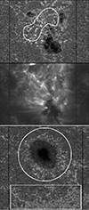 |
Fig. 1. Examples of reconstructed spectroheliograms from IRIS dense large rasters. Top panel: AR observed on February 4, 2016, at 2800 Å. Middle panel: Same AR image obtained in the intensity integrated over the Mg II k domain (±1.25 Å). The CBs in this AR have been assigned to an EMF region marked with a white contour. Bottom panel: AR on March 24, 2016, at 2800 Å. The white circle indicates a sunspot area, whereas the rectangle is a plage area. |
Our goal was to find various kinds of CBs visible in different ranges of Mg II h and k lines. We defined three criteria to determine the values of contrasts in specific wavelengths. The contrast is defined as follows:
 (1)
(1)
where ICB is the intensity in one specific wavelength or the average intensity in the wavelength range determined for a CB profile, IQS is the relative intensity obtained from the reference quiet Sun profile. Each phenomenon had to pass at least one contrast criterion. Below, we present our three criteria with a number of passed CBs corresponding to each ofthem:
-
CBs with a contrast greater than 2 at 2800 Å: 1835 CBs found.
-
CBs with a contrast greater than 9 in integrated and averaged. intensity of Mg II k line in range between −1.25 and +1.25 Å from the line center: 499 CBs found.
-
CBs with a contrast greater than 6.5 in integrated and averaged intensity of Mg II k line in range between −1.25 and +1.25 Å from the line center and simultaneously a contrast greater than 1.5 at 2800 Å: 616 CBs found.
Such wavelength ranges were chosen to find as many phenomena as possible. At 2800 Å, which is in the middle between the h and k lines, we can very often observe the maximum intensity in the Mg II k wing. On the other hand, the ±1.25 Å range allows us to find phenomena with increased intensity in peaks or in the line center (which is much rarer). However, the maximum intensity of most CBs is located somewhere in a spectral range of ±1.25 Å.
To calculate the contrasts, we need to know the values of the quiet Sun intensity. For each raster, we selected an area where no active structures were visible. Then we determined an average Mg II h and k quiet Sun profile to serve as our reference profile. It allowed us to calculate the contrast for each pixel at any wavelength. Based on the search criteria, we created contrast maps highlighting areas where the pixels met the specified conditions. The next step involved identifying the local maximum within a 7 × 13 pixel area (a rectangular region resulting from spectroheliogram deformation, given the spatial resolution of the IRIS pixel of 0.33″ on the x axis and 0.167″ on the y axis). This local maximum was recognized as the center of a CB. Finally, the CBs were visually verified for the following issues:
-
Compact structure and size – some of the events are diffuse and not so distinct. We chose brightenings with sizes ranging from ∼9 px (∼0.5 arcsec2) to 200 px (∼3 arcsec2) with a bright kernel inside.
-
Repeated events, which happen in two situations: in the case of larger events, the algorithm could take two positions for one event (two local maxima in the area of one event), and in the case in which one event was found using two criteria (different pixels but from the same event) we took the average value for the parameters.
-
Phenomena considered as micro-flare events (53 found).
During verification, we encountered some problems with significantly elongated phenomena found by the algorithm. We decided to exclude such structures, considering the possibility that they may be associated with flares. Our objective is to focus on phenomena occurring in the lower solar atmosphere that could be interpreted as magnetic reconnection events.
3.2. Characteristics of the Mg II profiles
The automatic procedure found 2950 CBs in 170 rasters, 2053 CBs were selected for further analysis after visual inspection. Each CB in our analysis is represented by a one-line profile extracted from the Mg II k spectra. Using this line profile, we calculated a set of parameters that allow us to define, describe, and compare all CBs. Since the Mg II h and k lines are formed throughout the entire chromosphere, they are excellent diagnostic tools for assessing its physical conditions. Variations in temperature, velocity, or density are reflected in the complex shapes of the Mg II line profiles. Line center (h3, k3) form in the upper chromosphere, around 2500 km, emission peaks (k2, h2) around 1500 km in the chromosphere (above the place in atmosphere were τ500 = 1, Pereira et al. (2013a)), whereas wings of the Mg II h and k around the TMR and deeper. Leenaarts et al. (2013a,b), Pereira et al. (2013a), Ondratschek et al. (2024) studied some statistical relations between plasma condition and Mg II h and k line profile parameters (for example: peak intensity, peak separation, line center intensity, profile width, and Doppler shifts) based on a quiet chromosphere simulation. They found some interesting relations between k2, h2 peak intensity, and temperature, or line width and chromospheric velocities. Another interesting conclusion was a correlation between peak separation and the absolute value of the difference between the maximum and minimum atmospheric velocities in the area between the formation region of the peaks (k2) and the line center (k3). Such results justify the use of the Mg II h and k line for probing chromospheric conditions. For studying CBs, we chose a set of parameters (similar to those in Grubecka Litwicka et al. 2016) related to different parts of the Mg II h and k line profile, which we identified as proxies for plasma conditions and formation height. Some of the selected parameters are related to those studied in the works of Leenaarts et al. (2013b), Ondratschek et al. (2024), such as peak separation. For other important profiles points, we used contrasts instead of intensity (in line center (k3), in peak (k2)).
All parameters were calculated for the Mg II k line (all rasters included the spectral range around Mg II k, some also covered the Mg II h line). However, since the Mg II h and k are formed under the same physical conditions, the results presented for Mg II k can easily be extended to the Mg II h line.
The parameters for the Mg II k line were computed asfollows:
![Mathematical equation: $$ \begin{array}{ll} C_{c}&\text{ k} \text{ line} \text{ center} \text{ intensity} \text{ contrast} \text{(k}_3\text{)} \text{[line} \text{ center} \text{ contrast].} \\ C_{P}&\text{ k} \text{ line} \text{ peak} \text{ intensity} \text{ contrast} \text{(k}_2\text{)} \text{[peak} \text{ contrast].} \\ C_{L}&\text{ Average} \text{ intensity} \text{ contrast} \text{ in} \text{ range} \text{(}\pm 1\,{\AA }\text{)} \text{ of} \text{ k} \text{ line} \text{[line} \text{ contrast].} \\ C_{+1}&\text{ Contrast} \text{ at} \text{+1}\,{\AA } \text{ from} \text{ k} \text{ line} \text{[close} \text{ wing} \text{ contrast].} \\ C_{2800}&\text{ Contrast} \text{ at} \text{2800}\,{\AA } \text{[far} \text{ wing} \text{ contrast].} \\ C_{\rm TL}&\text{ Contrast} \text{ at} \text{ center} \text{ Mg} \text{ II} \text{ UV} \text{ triplet} \text{(2798,8}\,{\AA }) \text{[triplet} \text{ center} \text{ contrast].} \\ C_{\rm TW}&\text{ Average} \text{ contrast} \text{ at} \text{ wing} \text{ of} \text{ Mg} \text{ II} \text{ UV} \text{ triplet} \text{(}\pm 0.15\,{\AA }\text{)} \text{[triplet} \text{ wing} \text{ contrast].} \\ FWHM_{\rm Mg}&\text{ Full} \text{ width} \text{ at} \text{ half} \text{ maximum} \text{ of} \text{ Mg} \text{ II} \text{ k} \text{ line} \text{ determined} \text{ by} \text{ fitting} \text{ of} \text{ Gaussian} \text{ function} \text{[}{\AA }\text{].} \\ I_{\rm Mg_{max}}&\text{ Maximum} \text{ intensity} \text{ of} \text{ Mg} \text{ II} \text{ k} \text{ line} \text{[DN/s].} \\ P_{\rm Sep}&\text{ Separation} \text{ peak} \text{ of} \text{ Mg} \text{ II} \text{ k} \text{ line} \text{[km/s].} \\ \end{array} $$](/articles/aa/full_html/2025/08/aa53134-24/aa53134-24-eq2.gif)
For a more simplified description of each parameter, we added in the square brackets short names that we are using along the present paper, for example: in this paper we call “average intensity contrast in the range ±1 Å of the Mg II k line” as just “line contrast.” In Figure 2, we marked with vertical lines particular wavelengths for which the parameters listed above were determined. The line center contrast is calculated for wavelength 2796.35 Å (k3), the peak contrast (CP) is determined for the stronger of the two peaks of Mg II k line (k2). We also determined the contrast for the Mg II UV triplet – both wing and center (description in Sect. 5.2). To calculate the full width at half maximum (FWHM) of the Mg II k line, we fit each profile with a Gaussian function. IMgmax was determined by searching for the maximum value of intensity in the range ±1 Å from the Mg II k line center. This parameter was useful in comparison with Si IV and C II emission.
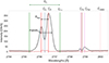 |
Fig. 2. Mg II k and Mg II UV 2 and 3 triplet lines profile. Vertical lines indicate particular wavelengths for which we determined different line parameters defined in Sect. 3 and listed in Table 2. The vertical blue line indicates the k line center and the two vertical red lines the k line peaks. The green are at ±1 Å from k line center. The vertical orange line is at 2800 Å. The vertical brown line and the two pink lines are centered, respectively, at the triplet Mg II UV center and the wings at 0.15 Å. |
Mean values and standard deviation of CB parameters.
In Table 2 we present the averaged parameters calculated for all CBs. The standard deviation is large for some parameters, which may be interpreted by the different shapes of the profiles. The deviation of Cc and CL can be due to non-reversed profiles, and C+1 due to large enhancements in the wings of Mg II.
4. Classification of CBs
Compact small-scale phenomena observed in the Mg II h and k lines present various spectral properties. They can be classified according to the contrasts at different wavelengths. One of our goal was to classify similar events, which allows us to analyze them more effectively. We adopt the same classification system of Mg II CBs as in Grubecka Litwicka et al. (2016). The 2053 CBs are divided into three types according to the shape of the Mg II k line profile:
-
Type 1: CBs with strong emission only in Mg II line peaks or in line center.
-
Type 2: CBs with emission observed both in the line peaks and line wings (emission raised in the broad spectral range).
-
Type 3: CBs showing enhanced emission only in the far wings of Mg II h and k lines.
In Figure 3 we present some examples of Mg II line profiles for all three types of CBs. Following Grubecka Litwicka et al. (2016) we may attribute to each CB type its average formation height. The NLTE modeling presented in Grubecka Litwicka et al. (2016) defines for each type a 1D model, in which the CB is represented by an enhancement of temperature localized at a specific height in the atmosphere (hot spot or temperature bump). For Type 1, the bump is formed above the TMR; for Type 2, exactly in the TMR; and for Type 3, below this area, close to the photosphere. Because in Grubecka Litwicka et al. (2016) they fit only five profiles of CBs with five different 1D models, it could appear an unjustified assumption to use this result as a general view. However, these five profiles are highly representative of the three profile types, and we will rely on this assumption in the discussion.
 |
Fig. 3. Examples of profiles for the different types of CBs. Left panel – Type 1 with strong line emission (black profile for Type 1B, red profile for Type 1N). Middle panel – Type 2 with excess emission in a wide range. Right panel – Type 3 CB profile with emission only in the far wings. Blue profiles show a quiet Sun profile. Black and red indicate the profiles of the analyzed CBs. Below the profile plots, we also present the corresponding spectra. In the case of Type 1, we present spectra of the red profile of Type 1N. |
4.1. Algorithm based on the definition of the contrast R
To automatically classify the 2053 CBs into three profile types, we developed a simplified algorithm. It is challenging to categorize the phenomena into different types, as there are no sharp boundaries between the characteristics of CBs. The types transition smoothly from one to another, since the observed events occur at varying heights, span different energy ranges, and can be triggered by different mechanisms. This classification into types is therefore conventional, serving primarily as a tool to narrow down the events, better understand their properties, and identify behavioral patterns. Our classification is based on the shape of the Mg II k line profile. We aim to identify a characteristic coefficient that can represent each profile type. To construct this coefficient, we used two parameters: far wing contrast and line center contrast. Since these values correspond to different parts of the spectrum, they may serve as effective diagnostic tools for classification. We defined a new coefficient as a ratio of two contrast values: in the far wing (at 2800 Å), and in the line (contrast for the average intensity in the range ±1 Å of the center of the k line). This coefficient (R = C2800/CL) describes the relationship between particular parts of the line profile.
In radiative transfer theory, this coefficient is also of significant interest. Using 243 atmospheric models with a hot spot, constructed in Berlicki & Heinzel (2014), we identified a relationship between the coefficient R and the height of the hot spot in a 1D model atmosphere. Figure 4 presents a theoretical diagram illustrating the relationship between coefficient R and the formation height of the hot spot.
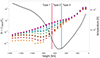 |
Fig. 4. Theoretical relation between the ratio of R = C2800/CL, (left side of y axis) and formation height of CBs above the photosphere computed using the grid of 243 models (Berlicki & Heinzel 2014; Grubecka Litwicka et al. 2016). Each color represents a different formation temperature from 1100 K (orange, the lowest dots) to 5500 K (pink, the highest dots), with a step of 550 K. Two vertical lines indicate approximately the boundary heights of the formation for three different types of the CBs studied in Grubecka Litwicka et al. (2016). Type 1 CBs form on the left of the red line, Type 2 CBs between the green and red lines, and Type 3 CBs on the right side of the green line. In addition, temperature profile (right side y axis) from VAL C model atmosphere (Vernazza et al. 1981) is overplotted with a solid black line. |
For events formed high in the chromosphere, characterized by strong emission in the Mg II k line and little to no emission in the far wings, the R coefficient takes on low values. In contrast, for events without line emission but with significant wing emission (Type 3), R is much greater than 1. For Type 2 events, which show comparable emission in both the line core and the wings, R takes intermediate values. For CBs studied in Grubecka Litwicka et al. (2016), R took the following values: CB A: R = 0.13, CB B: R = 0.07, CB C: R = 0.58, CB D: R = 0.40, CB E: R = 1.55. Based on the values above, we arbitrarily adopt the following thresholds to distinguish between the three types:
-
R < 0.25 – Type 1
-
0.25 < R < 0.9 – Type 2
-
R > 0.9 – Type 3
Therefore, we could draw some height limits in Figure 4 for the three types of CBs that we use in our conclusion. Further, in the paper, we consider R as a proxy of height in the atmosphere. The higher the height in the atmosphere, the lower theR is.
4.2. Statistical characteristic of the CBs
We computed the R ratio for all 2053 identified CBs and obtained 556 Type 1 CBs (27%), 1096 Type 2 CBs (53%) and 401 Type 3 CBs (20%). Approximately half of the CBs are Type 2. In Table 3, we present the mean values and standard deviations of different parameters defined in Sect. 3.2, determined separately for three types of CBs.
Mean values and standard deviation for three CB types’ parameters.
For Type 1 CBs, we observe high contrast in the line, at the line center, and in the peaks. Additionally, FWHMMg and PSep show significantly higher values compared to the other types. Type 1 CBs also exhibit the highest contrast values in the close wings (±1 Å), which in most cases correspond to broad and extended line profiles (Figure 3, left panel). We can note that the parameters related to the central parts of Mg II k lines tend to have higher values than the other contrast parameters, likely due to their strong sensitivity to temperature increases, particularly in the Mg II k peaks. Type 2 CBs, as an intermediate type, have less dispersed parameter values. For this type of event, enhanced emission is observed across the entire Mg II k line profile (Figure 3, middle panel). For Type 3 CBs, the parameters of CC, CL, and C+1 have very low values; however, C2800 has high contrast values (Figure 3, right panel).
In Figures 5 and 6, we present histograms of the Mg II k line parameters listed in Table 3. Figure 5 (upper panel) presents the scatter plot of two parameters, C2800 and CL used for the classification, and the histograms of these two parameters (two lower panels). In the correlation diagram (top panel), we note some global anticorrelation (Pearson’s linear correlation coefficient RP = −0.49) with a general tendency that increasing line emission is related to decreasing wing emission. However, when considering CBs of specific types, particularly types 2 and 3, we observe a positive correlation: higher contrast values of C2800 tend to correspond to higher contrast values of CL. This suggests that stronger phenomena simply present larger values of individual parameters, while maintaining a similar ratio, R, of C2800 and CL. Type 1 CBs are the most dispersed in the top diagram; Type 2 CBs, which are the more numerous, display only a minor scatter, similar to Type 3 CBs. This behavior among the three CB types is also evident in the histograms in Figure 6, which clearly illustrate the distributions of individual parameters such as CC, CP, C+1, PSep.
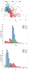 |
Fig. 5. Top panel: Correlation plot showing the relation between the contrast at 2800 Å (C2800) and the contrast in the mean contrast in the Mg II k line (CL). Middle panel: histograms of C2800. Bottom panel: Histogram of CL. Type 1 CB is in red color, Type 2 CB is in blue, Type 3 CB is in green. In the top panel we note a global anticorrelation with a general tendency that increasing line emission leads to decreasing wing emission. The diagonal gray lines indicate the values of the ratio, R (0.25 and 0.9), which separate the three types of CBs. Black dots indicate the five CBs from paper Grubecka Litwicka et al. (2016). |
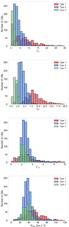 |
Fig. 6. Histograms of four parameters; contrast in the line center, contrast in stronger peak of Mg II k, and contrast in close wing and peak separation. |
The studied CBs have been divided into three types based on similar spectral characteristics; however, the Mg II profiles within each type exhibit a wide variety of shapes. After visually inspecting numerous CBs of each type, we identified additional distinguishing characteristics. For Type 1 CBs, we observe the greatest variation in the Mg II k line parameters. Most notably, these profiles show strong emission near the Mg II h and k lines and weak emission in the far wings (see the histogram of C2800 in Figure 5). One note that Type 1 CBs show a clear bimodal distribution, which is also visible in the scatter plot (Figure 5, top panel). Such a distribution shape may suggest two distinct groups of phenomena among Type 1 CBs. Less pronounced, but also bimodal is the distribution of the CL, PSep, or CC parameters. Because we took the brightenings with strong integrated line emission, we obtained two subtypes; one subtype with very strong and narrow peaks (N subtype) and a second with very broad h and k lines (B subtype). Probably, because of these two subtypes, the histogram of C+1 shows a very broad range of values, with a ragged plateau and no clear maximum. N subtype CBs have a huge intensity increase in the Mg II k line and a small, or comparable to the quiet Sun emission in the far wings. These events sometimes present only one peak instead of two peaks with very shallow self-absorption in the line center. For some events with strong narrow Mg II k line, the emission in the triplet Mg II UV center appears, sometimes also in the wing. Second B subtype CBs are phenomena with very broad and more complicated profile shapes with extended wings and emission in the far wings, very often with superimposed absorption features. Presence of such lines may indicate lower location of CBs, where the photospheric absorption lines are formed (Peter et al. 2014). These are phenomena among which emission in triplet is very likely to appear (see Sect. 5.2).
Taking into account the histogram of PSep, the highest values of peak separation had Type 1 CBs and slightly less frequently Type 2, reaching up to 120 km/s, with a mean value for Type 1 CB 52 km/s. For the quiet chromosphere, the peak separation is typically between 10 and 40 km/s (Pereira et al. 2013b). Such a large spread of values compared to the values from Pereira et al. (2013a) may indicate more dynamic plasma motions in active phenomena than in the quiescent chromosphere. For all CBs PSep and formation height, related to the value R, show a weak negative correlation (Spearman correlation coefficient RS = −0.34). We also noticed a similar correlation for theoretical profiles – the largest peak separations were present for phenomena formed between 600–800 km; that is, at the boundary between type 1 and type 2 CBs. In the case of synthetic profiles near TMR, the large PSep was related to strong emission in the near wings, covering and broadening emission peaks, rather than plasma velocities, which were not included in our radiative transfer calculations. Moreover, the theoretical profiles of Mg II k lines are generally narrower and have much less peak separation than those observed (Leenaarts et al. 2013b; Grubecka Litwicka et al. 2016; Rubio da Costa et al. 2016; Ondratschek et al. 2024). Therefore, observations should not be directly compared with modeling results, but it is worth noting a common trend associated with large peak separation for CBs originating in the vicinity above, but close to TMR. However, some of the extreme values may be due to misidentification of peaks by the algorithm, due to the highly irregular and complex shape of the Mg II k line profile.
For 20% of Type 1 CBs there are no superimposed absorption features, sometimes we can only see shallow absorption lines. This can be interpreted as evidence for the formation height of Type 1 CBs in the higher chromosphere. Especially, for those 20% CBs mean R = 0.05, while for Type 1 CBs, with absorption characteristics, R = 0.14.
Type 2 CBs are the most numerous events. This type CBs have very similar enhanced emission in the Mg II wings but also in the close wings – this makes the line wider, while the emission in the wings from +1 to +3.5 Å is significantly increased. A large number of events exhibit double peaks in the Mg II lines, all of which have superimposed absorption features from neutral atoms. Type 2 CBs display more diverse and asymmetric profiles compared to Type 3. Additionally, a larger fraction of Type 2 events (27.2%) show emission in the Mg II UV triplet, though this emission is mostly in the wings, with only a slight enhancement at the triplet line center. The distributions of all parameters are distinctly unimodal, with values clustered closely around the mean.
Type 3 CBs form a very uniform group and differ only in details. All of them have very narrow Mg II h and k lines with self-absorption in the line center (only four events have one peak). The standard deviation of FWHMMg is quite low (0.31 Å). Strong emission occurs only in the far wings of Mg II h and k lines, greatest in the middle between h and k lines. The emission in the Mg II UV triplet line at 2798.809 Å is described in detail in Sect. 5.2. All Type 3 CBs profiles exhibit superimposed absorption features, similar to those in Type 2 CBs. These features are generally deep and always clearly visible. The absorption primarily originates from neutral atoms, such as Mn I and Fe I.
The analysis of CB characteristics focuses on the shapes of the Mg II h and k lines. In the following sections, this classification is further extended by examining the relationship of the phenomena with other line emissions (Sect. 5), their location within ARs (Sect. 6), and their association with related phenomena (Sect. 7).
5. Correlation of CBs with other line emission
5.1. Emission in FUV
A significant number of NUV CBs are also visible in the far UV (FUV) within our rasters. The strongest lines in the FUV spectral range are the Si IV doublet at 1394 Å and 1403 Å, and the C II resonance multiplet at 1334.53 Å, 1335.66 Å, and 1335.70 Å. Both multiplets are formed at much higher temperatures than the Mg II h and k lines–approximately 4⋅104K for C II and 8⋅104K for Si IV (Peter et al. 2006). The simultaneous emission in all three lines remains a puzzling phenomenon. In this study, we investigate how frequently this common emission occurs and which types of phenomena it is associated with.
In our research we are using spectra of Mg II h and k, Si IV, and C II from 170 rasters. Most of them have available both 1394 Å and 1403 Å spectral lines. However, for 20 rasters, only one Si IV line, either 1394 Å or 1403 Å, was available for analysis. We chose to prioritize the line that appeared more frequently in the raster data. Si IV 1394 Å was unavailable for 193 events, while Si IV 1403 Å for only 132 events, making the latter our default choice. For the 132 CBs visible only in the 1394 Å line, we scaled the derived parameters to allow for a comparison with the ones based on the 1403 Å line. Under optically thin conditions, the integrated intensity ratio of these two lines is 2, with the 1394 Å line being the stronger one (Peter et al. 2014). However, due to opacity effects, strongest at the line center and weaker in the wings, the Si IV line ratio depends on wavelength and falls below 2 at the line center (Zhou et al. 2022). Such deviations from the expected ratio indicate that line formation does not occur under optically thin conditions and that optical depth effects play a significant role in the process (Kerr et al. 2019; Tripathi et al. 2020). The ratio often falls between 1.8 and 2.3. For the 698 events in which emission from both Si IV lines was observed, we determined the mean Si IV intensity ratio calculated in the line center, which turned out to be 1.82 (with a standard deviation equal 0.4). We used this value and rescaled Si IV 1394 Å profiles to get an estimation of the intensity of the Si IV 1403 Å line.
Initially, all CB events were divided into two groups: those with emission in the FUV lines and without. Events exhibiting relatively strong Si IV and C II emission, with maximum intensities exceeding 70 DN/s, were automatically classified as “with emission.” For weaker events, we determined the classification based on the following criteria:
-
Mean intensity I±0.2 Si IV and C II lines in the range of ±0.2 Å from the line center,
-
Mean intensity Isurr and its standard deviation σsurr coming from nearby surroundings of each line,
-
Quiet Sun emission derived in the same way as for Mg II k line.
In the case of Si IV values of Isurr and σsurr were determined in the spectral range 1403.3–1403.9 Å or 1392.5–1393.1 Å, depending on which line was available. For C II line values of Isurr and σsurr were calculated in the range: 1336.3–1337.0 Å. The classification is based on the following criterion:

Analyzed events were classified as “with emission” when the above criterion was met and the intensity I±0.2 of the CBs exceeded the quiet Sun emission. The results show that nearly 73% of all CBs exhibit a response in the C II lines, while approximately 55% show a response in the Si IV lines. Table 4 summarizes the number of CBs with emission in Si IV and C II, divided according to the three CBs types. Among Type 1 CBs, almost all display FUV emission (96.4% in Si IV, 99.4% in C II). This percentage decreases for Type 3 CBs, where only 15.4% exhibit Si IV emission. This discrepancy may be due to the lower formation temperature of C II compared to Si IV. The Mg II h and k lines and C II form closer to each other in the atmosphere than Mg II h and k and Si IV lines.
Emission in FUV lines.
Further detailed analysis required some parameters of Si IV and C II, which are:
-
FWHMSi – full width of half maximum [Å]
-
ISimax – maximum Si IV intensity
-
ISimean – average intensity of Si IV in the range ±1.3 Å
-
ICmax – maximum C II intensity
-
ICmean – average intensity of C II in the range ±0.6 Å
Some of the statistical results are presented in Figures 7 and 8, as well as in Table 5. For Type 1 CBs the emission in hotter lines is quite common, the correlation between the emission in the Mg II h and k lines, and FUV lines is evident. In Figure 7 (middle panel), we present correlation plot of CL and ISimean (correlation coefficient RS = 0.6, see Table 5). The bottom panel of Figure 7 shows a scatter plot of the ratio, R, which represents the atmospheric height, against ICmean. The colors of the data points indicate the logarithm of ISimean, as shown by the color bar on the right. There is a clear anticorrelation between the emission in the FUV lines and R. The Spearman correlation coefficients (RS) for R and ISimean or ICmean, are −0.71 and −0.76, respectively. It is noteworthy that C II or Si IV emission in Type 3 CBs is rare and weak, but still significant given the low formation height of these events. Also puzzling is the FUV emission observed in approximately half of Type 2 CBs, especially considering their origin in a relatively narrow TMR. We observe a general trend: CBs exhibiting FUV emission tend to have higher mean values of all Mg II k line parameters compared to those without such emission within each type. This suggests that stronger events are more likely to show FUV emission. However, this does not explain why some strong events show no response in the Si IV and C II lines, while some weaker CBs do. There are approximately 700 CBs with IMgmax greater than 200 DN/s, yet 30% of them do not exhibit Si IV emission. On the other hand 10% of CBs with IMgmax less than 100 DN/s (with far wing and close wing contrast greater than 1.4) do show Si IV emission. There are three possible scenarios to explain this discrepancy: 1) There may be a temporal offset between emissions in different lines, and we are observing only a single moment in the lifetime of each event. 2) The temperature might be high enough to generate emission in hotter lines, causing Mg II to become mostly ionized, resulting in weak or absent Mg II emission (possibly originating from below the CBs). 3) Additional physical conditions may be required to produce FUV emission.
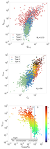 |
Fig. 7. Upper panel: Correlation plot of C+1 and ISimean for three types of CBs. Middle panel: Correlation plot of CL and ISimean. With black circle edges, we mark CBs related to UV bursts, and with yellow possible EBs (more in Sect. 7). For the first two plots, colors of points refer to three types of CBs. Bottom panel: Correlation plot of ratio, R (C2800/CL, which relates to the atmosphere formation height (Fig. 4) and ICmean. Colors on this plot represent values of logarithm of the ISimean, according to color bar on the right side. Two vertical lines indicate the edges between three types of CBs (defined by C2800/CL), which are marked with the numbers “1,” “2,” and “3” at the top of the plot. |
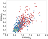 |
Fig. 8. Correlation plot shows relations between FWHMMg and FWHMSi for all CBs with FUV emission greater than threshold values. The Pearson coefficient describing linear relations is equal to 0.78. The red color represents Type 1 CBs, blue Type 2, and green Type 3. |
The correlation is observed not only between emissions in different lines, but also between their profile widths. The calculated Spearman correlation coefficient between FWHMMg and FWHMSi is equal to 0.8, suggesting that the two lines may form under similar physical conditions. Furthermore, the Spearman coefficients between R and FWHMMg or FWHMSi are −0.61 and −0.66, respectively. This indicates that the Si IV profiles become narrower as we move from Type 1 to Type 3 CBs, i.e., deeper into the atmosphere. A similar trend is observed for the maximum intensity, which also decreases (see Table 5).
Values of the FUV lines parameters.
We calculated the linear Pearson’s correlation coefficients (RP) between CBs average intensity in Si IV and other Mg II k line parameters (Table 6). ISimean shows the strongest correlation with C+1, with a Pearson correlation coefficient RP = 0.73 for all CBs. The correlation is even stronger for Type 2 CBs, reaching RP = 0.83 (see upper panel of Figure 7). This correlation may reflect conditions in the line formation region. High C+1 are typically associated with broad Mg II k peaks, as broader peaks tend to have their maxima shifted toward +1Å. Such a broadening may result from local plasma motions (Ondratschek et al. 2024) or from a sudden increase in plasma density, which enhances opacity in the Mg II h and k lines. Both scenarios are indicative of dynamic and intense processes, which in turn may increase the likelihood of strong Si IV emission. Additionally, these observations suggest the possibility of a shared or overlapping formation region for Mg II k and Si IV emission. The RP values for C2800 are particularly interesting. When calculated separately for each CBs type, RP shows a slight positive correlation, suggesting a weak relationship. However, when computed across all CBs, the result is a very weak anticorrelation (RP = −0.07). This discrepancy can be explained by the overall trend observed across the three CB types. Within each type, where the formation region is relatively consistent, a higher C2800 value likely corresponds to stronger events, and thus a higher probability of FUV emission, resulting in a positive correlation. However, when considering all CBs together, the trend reverses: CBs that show strong Si IV emission tend to form higher in the atmosphere, where C2800 values are generally lower, resulting in an overall anti-correlation. The lowest RP values are found for CC. While one might expect a correlation between Mg II k line center emission and Si IV, particularly for Type 1 CBs, the data show that RP is close to zero. This may be due to the influence of the overlying canopy, which affects CBs radiation in the Mg II k line center, as extensively discussed in Grubecka Litwicka et al. (2016). An analogous analysis of Mg II k line parameters and C II emission yields similar conclusions; therefore, we do not present the correlation coefficients for C II here.
Pearson correlation coefficients.
5.2. Mg II UV triplet
Mg II UV triplet of subordinate lines (2791.6 Å, 2798.75 Å, 2798.82 Å) constitutes a remarkable diagnostic tool, but unfortunately they are not frequently discussed in a literature. Figure 9 displays a few examples of triplet emission profiles and spectra in different types of phenomena. These lines are formed in the same regions in the solar atmosphere as the Mg II h and k lines and, generally, are much weaker from them. In most cases, they appear as absorption lines, but in the case of energetic events, they become emission lines (Pereira et al. 2015). Our goal is to examine in which events exactly emission in triplet occurs, both in line center and wings. We are interested in looking at the correlation with other CB parameters. Triplet Mg II UV emission in the 2798.8 Å line occurs mainly for CBs with stronger emission in h and k lines (strong peaks), but is rare for events with emission only in the far wings. We often observe emission in the wings of the Mg II triplet lines with absorption in the line center at 2798.8 Å, more frequent for CBs of Type 1 and 2. There are also some CBs among Type 1 with strong emission in the Mg II h and k lines, often without self-absorption in the peaks, and with additional emission in the center of UV triplet lines. These events often exhibit very low contrast values in the far wing. In many cases, Mg II h and k and Mg II UV triplet line profiles exhibit similar shapes, for example, showing comparable asymmetry or line width. The modeling results of the Mg II UV triplet lines (Pereira et al. 2015) indicate that when heating occurs deeper in the atmosphere and is overlain by cooler material, the emission in the triplet lines appears predominantly in the far wings, while the central part shows absorption, accompanied by broader Mg II h and k profiles. Conversely, when heating takes place at higher atmospheric layers, the emission is centered in the line center. These findings are consistent with our observations and analysis.
To examine the emission in triplet Mg II UV lines, we first determined two values – the triplet line center intensity (ITC) and the average triplet wing intensity (ITW). It is reasonable to compare these values with the intensity measured near the triplet line center, so we used the nearby intensity at 2800 Å (I2800). We determined the presence of emission in the Mg II UV triplet lines when the intensity in the triplet wing or line center exceeds that at 2800 Å (ITC > I2800 and ITW > I2800 ). So, basically, we checked if the triplet emission is enhanced enough to be visible. We introduced two indicators of the triplet emission:
-
TC = ITC/I2800
-
TW = ITW/I2800.
For the quiet Sun, the Mg II UV triplet line emission is not enhanced, so TW = 0.8 and TC = 0.3 (average values calculated for the quiet Sun profiles for all rasters). In the case of triplet emission, we expect values greater than 1, thus we set this value as a threshold for evaluation of the triplet emission presence. When TW > TC then we observe triplet wing emission, in the case of TW < TC we have triplet line center emission. Using this method, we received the following statistic: 750 of the phenomena (36.5%) have an enhanced emission in the triplet line wing (721) or center (29). We found that 391 (70.3%) of Type 1 CBs exhibit an emission in triplet line wings and 29 CBs (5.2%) present an emission in the triplet line center. In Figure 9, we present representative examples of triplet line emission for Type 1 and Type 2 CBs. For Type 3 CBs, the triplet lines appear mostly in absorption; however, the right panel of Figure 9 shows a rare example of triplet line wing emission. We have also calculated contrast values for the triplet line center (CTC) and the average triplet wings (CTW), following Equation (1). The values of these two parameters for all CBs are provided in Table 2 and for particular CBs types in Table 3. The largest value of CTW is found for Type 2 CBs, whereas CTC for Type 1. We found some relationship between the triplet and FUV emission. Among all CBs, regardless the type, events presenting emission in triplet line wings or center have simultaneously greater values of ISimean, ISimax, ICmean and ICmax parameters, than CBs without triplet emission. It appears that enhanced triplet emission is associated with stronger emission in the FUV. This is well visible in Figure 10, where we present two correlation plots of the R coefficient, representing the CB types and with, respectively, CTC (upper panel) and CTW (bottom panel). The colors in these plots represent the logarithm of ISimean, as indicated by the color bar. Based on the relation between R and CBs formation height, we can check how triplet emission relates to location in the atmosphere. Clearly, line center triplet emission is more frequent for Type 1 CBs and drops for Type 2 and Type 3. The opposite situation is found for CTW, which increases with increasing R, and the largest CTW values are observed for Type 2 CBs. Moreover, among particular types of CBs, ISimean takes higher values for CBs with larger CTC and CTW. Similar correlations were also found for the ICmean parameter.
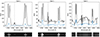 |
Fig. 9. Examples of different triplet emission (indicated by the vertical dashed line) among particular types phenomena. Triplet emission for Type 1 is very distinct, with clear similarity to Mg II h and k line, emission appears also in triplet line center, but still we observe central absorption. The middle panel presents triplet emission for Type 2 CBs with strong emission in wings (sometimes even stronger than in the Mg II h and k line). This type of emission appears also in Type 3 (right panel). Below profiles we are showing corresponding spectra. |
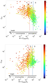 |
Fig. 10. Upper panel: Correlation plot of ratio, R, and CTC. Bottom panel: Correlation plot of R and CTW. The ratio, R (C2800/CL), relates to the atmosphere formation height (Fig. 4). The colors in both plots represent values of logarithm of the ISimean, according to the color bars on the right side. Two vertical lines separate three different types of CBs (defined by C2800/CL), which are marked with the numbers “1,” “2,” and “3” at the top of each plot. |
6. Location of CBs in active region structures
In all 170 rasters we identified different types of AR structures, among which we distinguish three main types (Figure 1): a) emerging magnetic flux (EMF) region, b) area close to sunspot penumbra, and c) plage regions. There were also some remaining CBs that cannot be classified in any of these area types. We attributed them to so-called “isolated areas.” When an AR showed several types of structures, each CB belonging to given structure was classified to this particular type. An EMF region is defined as an area with a strong bipolar magnetic field visible on HMI magnetograms. Plages are hot and wide areas with no other structure. Sunspot area CBs are located around (up to 1 radius of) a sunspot, close or in penumbra. Isolated CBs are distant from other events, in regions located far from active structures. Our purpose was to determine which kind of AR structure produces the greatest number of a particular CB type.
Table 7 and Figure 11 present the results. EMF regions are the areas where CBs occured most frequently: 827 events came from EMF regions. There were 744 CBs counted in sunspot areas and 446 CBs in plages. Only 36 CBs were isolated from active structures in ARs. Table 8 presents the mean values of the selected CB parameters for different types of AR structures, with relatively small parameter dispersion. EMF regions produce the most energetic events, with the broadest line profiles, the strongest triplet and FUV emission (Table 8).
Number of brightenings in particular type according to AR type.
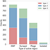 |
Fig. 11. Distribution of CBs among different AR types. One can notice that Type 1 CBs are forming mostly in EMF regions, Type 2 equally in EMFs, around sunspots and plages. Phenomena forming around sunspots come from Type 1 and 2. In plages Type 2 has the advantage. Isolated CBs come mostly from Types 2 and 3. |
Mean values of different CB parameters, according to their AR structure.
7. Relationship of CBs with other well-known small-scale phenomena
Over the years, many small-scale events have been defined in the literature, such as EBs (Ellerman 1917), IBs (Peter et al. 2014), and UV bursts (Young et al. 2018). We are very interested in searching for these kinds of small-scale phenomena among our CBs.
7.1. CBs as EBs
Small-scale reconnection events, originally referred to by Ellerman (1917) as solar hydrogen bombs, are now commonly known as Ellerman bombs. They are defined by the Hα line, their lifetime is several minutes, and they are around 2” in size. They appear mostly in the EMF region, as well as in sunspot moats, but were recently also found in the quiet Sun regions (Rouppe van der Voort et al. 2016, 2024; Nelson et al. 2017). Simultaneously, EBs observations in the Hα and Mg II h and k lines (Tian et al. 2016; Vissers et al. 2015) gave us evidence that EBs are also well visible in the Mg II k and k lines. This means that the Mg II h and k lines could be an additional, diagnostic tool for these events. Usually EBs in Mg II appear as strong events with broad, extended wings of h and k lines and absorption in the line center, similar to Hα. They also have increased emission in the far wings. What is also important, EBs profiles usually have superimposed absorption features such as Mn I, Fe I lines. These properties are summarized in Table 1 in Tian et al. (2016). In the paper mentioned above, it was also shown that EBs have no significant O IV (1401.16 Å) emission signatures. Based on confirmed EBs in Mg II h and k lines published by Vissers et al. (2015) and Tian et al. (2016) we analyzed EBs profiles to constitute criteria for Mg II k line contrast parameters. Our goal was to estimate the number of EBs from all the found phenomena. We constituted the following threshold values for different parameters:
-
FWHMMg = 0.75; The smallest FWHMMg of k line profile was 0.6, but it was only for a few events, most of EBs have a FWHMMg greater than 0.9, we adopted the value of 0.75.
-
Enhanced emission around 2800 Å, we adopted the threshold contrast value at 2800 Å equal 1.
-
Enhanced emission in close wing (+1 Å) with contrast at least equal 2.
-
Absorption in the line center.
-
Presence of superimposed absorption lines.
-
Lack or weak emission in O IV.
It should be mentioned that the EBs described in Tian et al. (2016) were connected to IBs, resulting in strong EBs. In Tian et al. (2016) paper the Mg II h and k profiles showed strongly enhanced peaks of the Mg II k line, with intensities greater than 400 DN/s. Since our goal was also to include weaker phenomena as possible EBs, we dropped the intensity criterion. It is important to note that we have no Hα observation for any of the CBs, so we cannot determine EBs with certainty 100%. However, satisfying the above criteria gives us a high probability of determining EBs. In the following sections, we use the term “EBs” in reference to the identified phenomena, yet, we must keep in mind that we are referring to probable EBs. Applying the above criteria to our set of 2053 phenomena, we identified 273 possible EBs (13% of all CBs) across 90 different rasters. They belong mostly to Type 1 (181 EBs), 88 EBs are from Type 2, and only 4 from Type 3. Among all EBs 76% have emission also in triplet lines. Almost all of them have response in FUV lines, 94% have signatures in Si IV and 99% in C II. We found that 179 (65%) EBs come from the EMF regions, 65 (25%) from the areas around sunspots, and 29 from the plage regions. Only 68 EBs have maximum Mg II k line intensity greater than 400 DN/s.
7.2. CBs as solar UV Bursts
In paper Young et al. (2018) the authors described and classified UV bursts phenomena, defined as a strong, small-scale, and short-lived reconnection event, visible in Si IV lines (and other transition region lines), with no signatures in coronal lines. This class of phenomena includes two subclasses of events – IBs and narrow-line bursts. They differ primarily in the width of their line profiles. Our research did not focus on the Si IV line, but it is very interesting to investigate how many NUV phenomena have a signature in more energetic lines. Because CBs are represented by line profile and spectra from one moment in time, we have limited ways to examine what kinds of phenomena represent particular CBs. Based on events published in Tian et al. (2016), Vissers et al. (2015) and the definitions from Young et al. (2018) we adopted a set of spectrum criteria that must be satisfied to consider CBs as UV bursts:
-
Minimum Si IV 1403Å intensity value: 200 DN/s.
-
Additional strong (more than 100 DN/s) emission in C II.
Using the above criteria, we found that 121 (6%) of CBs have signatures of UV burst emission. Significant part (62%) of these events came from the EMF area, 26% were located around sunspots, and 12% in a plage region.
7.2.1. CBs as IBs
The term IRIS bombs was introduced by Peter et al. (2014) and referred to strong and broad phenomena visible in Si IV lines, but also in C II and C I. Line profiles of IBs have superimposed absorption lines of neutral and singly ionized metals suggesting a low atmosphere formation height. These kinds of Si IV profiles were also observed in a magnetic reconnection site, producing a jet (Joshi et al. 2021). Absorption features in IBs were also studied by Kleint & Panos (2022), they found that for different IBs the depth of an absorption line varied. They attributed this to the formation height of the IBs, which is also consistent with our findings. We also observed a lack of absorption features in the highest-formed phenomena. Since neither intensity nor width were defined, we estimated these values based on published profiles of similar phenomena. Our IBs criteria for Si IV 1403Å are following :
-
Minimum intensity value: 200 DN/s.
-
Minimum FWHMSi: 0.6 Å.
-
Absorption lines presence.
-
Additional strong (more than 100 DN/s) emission in C II.
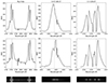 |
Fig. 12. Two examples of EBs being IBs at the same moment. This situation is rare: we found only 48 IB type events, 273 EB type events, and 28 phenomena that are both. For third row profiles, we additionally present spectra of the event. |
At this point, we want to add an explanation of how we evaluated the presence of absorption lines. Around 30% of the CBs were observed only in the Si IV 1403 Å line. It is known that the absorption feature near the 1403 Å line (Fe II 1403.1 Å) is shallower or does not appear, even if we see a strong absorption line close to Si IV 1394 Å (Ni II 1393.3 Å). Because we noticed a strong relation between absorption in C II and Si IV in our data, we decided to estimate the general presence of absorption features by also taking into account events in C II. Therefore, our condition for CBs to be classified as “with absorption” is to have visible absorption feature at least for one FUV line profile. Based on the above criteria, we found 48 IBs (2,4% of all CBs) in 27 different raster, 42 of the events we found were Type 1 CBs and 6 were Type 2. Emission in Mg II UV triplet lines was present for 78% of the IBs. In EMF regions we found 30 IBs, 14 in sunspot area and only 4 in plage region.
7.2.2. Narrow-line UV bursts
Narrow-line UV bursts (NUBs) are another type of small-scale phenomena and have not been described well in the literature (Hou et al. 2016). Such events are also difficult to distinguish from microflares. As NUBs, we understand strong events with a very narrow line profile. We adopted the same criteria as for UV bursts, with additional width criterion, which is that the FWHMSi is less than 0.3 Å. This FWHMSi value was estimated based on the profile published in Young et al. (2018). Using these two criteria, we identified 20 events across 16 rasters: 12 phenomena originated in EMF regions, and 4 were found in both sunspot and plage areas. Profiles for these kinds of events were similar for each of three spectral lines (Mg II, Si IV and C II). It seems that they are most likely formed higher in the atmosphere, where temperature-sensitive peaks of magnesium lines are formed.
7.3. CBs being EBs and UV bursts
In the middle panel of Figure 7, we present a scatter plot of CL and ISimean for three CBs types. This plot shows a general positive correlation between the emission in the Mg II k and Si IV lines for all CBs. With a black circle edge we marked UV burst events, with yellow possible EBs. One can see that they covered CBs with rather strong emission in the Mg II k and Si IV lines (mostly from Type 1 and 2). One of the most intriguing topics in small-scale solar activity research is the common emission observed in both FUV and NUV lines for compact phenomena such as EBs, UV bursts, and IBs. Several examples of simultaneous IB-EB type emissions are documented in the literature (Vissers et al. 2015; Tian et al. 2016; Chen et al. 2019a). The question of the atmospheric conditions and mechanisms producing these two events remains a puzzle for scientists. Based on evidence from EB modeling and the presence of absorption features, they are expected to form mainly in the lower atmosphere, where the temperature is much lower than the formation temperature of Si IV lines. Some articles have described scenarios in which certain circumstances can induce Si IV formation in a very dense and relatively cold environment. For example, Rutten (2016) claimed formation temperature around 1–2 ⋅ 104 K by applying Saha-Boltzman statistics (because of LTE assumptions), or Dudík et al. (2014) suggested low Si IV temperature formation by applying κ distribution of the electrons in modeling. Such scenarios seem reasonable, especially since such phenomena are quite rare.
Applying two sets of criteria, we were able to find how many CBs share signaturies of the EBs and IBs. In Figure 12 we present two examples of EB-IB phenomena visible in the Mg II h and k, Si IV and C II lines. We identified only 28 phenomena that meet the conditions relating to both IB and EB, which account for 10.3% of all EB and 58.3% of IB. This aligns with the conclusions from the other studies, where IBs represent 10–20% of all EBs, and 40–60% of IBs are associated with EBs (Chen et al. 2019a; Vissers et al. 2015; Tian et al. 2016).Examination of triplet activity in EB-IB events revealed that 90% of them exhibit significant triplet wing emission.
We could also look at the more general EB-UV burst relation. Of all CBs, 49 phenomena had EB and UV signatures, accounting for 40.5% of all UVs and 18% of all EBs.
8. Summary and discussion
We performed a statistical analysis of Mg II UV small-scale CBs based on the NUV and FUV spectra observed by IRIS, which is a continuation of the study by Grubecka Litwicka et al. (2016). The phenomena we are considering in this paper are a more general group of fine-scale UV phenomena, an extension of the solar UV burst class of events defined by the Si IV line profile (Young et al. 2018). Solar UV bursts commonly elicit a response in the Mg II h and k line, but there are many CBs visible only in Mg II h and k lines, without a signature in more energetic lines (Si IV, C II). That is why we focus primarily on the Mg II h and k line events.
In the first step of our analysis, we detected in a semiautomatic way the presence of CBs in 340 IRIS spectroheliograms, covering two different wavelength ranges: one around the Mg II k line center and the other in its far wings. We identified 2053 CBs showing strong emission, either in the far wings of the Mg II k line or within ±1.25 Å of the line center. To characterize these events in more detail, we classified the CBs into three types based on the ratio, R, of the two Mg II k line contrast parameters, C2800 and CL. The classification is as follows: Type 1 CBs form higher, above (> 650 km) the TMR, Type 2 around the TMR, between 480 and 650 km, and Type 3 CBs form lower than TMR (< 480 km). Additionally, we investigated how the Mg II k line emission relates to other spectral lines, namely, Si IV, C II, and the Mg II UV triplet, as well as the occurrence frequency of CBs across different types of ARs. Below, we briefly describe the characteristics of each CB type:
-
Type 1 CBs are the most diverse and account for 27% of all detected events. Almost all CBs of this type show signatures in both the FUV and Mg II UV triplet lines. They occur more frequently in EMF regions, and most IBs, EBs, and UV bursts fall into this category. Within Type 1, we distinguish two subtypes based on their spectral characteristics: the B subtype, which exhibits very broad emission peaks with extended wings, and the N subtype, characterized by strong emission in the narrow peaks and in the line center.
-
Type 2 CBs exhibit emission across the entire spectral range and account for 53% of all events. Half of them also show additional emission in the FUV and Mg II UV triplet lines. These events occur across various AR structures, appearing roughly equally in EMF regions, sunspots, and plages.
-
Type 3 CBs have highly uniform profiles and account for 20% of all events. For this type, emission in the FUV range is very rare, and the Mg II UV triplet lines typically appear in absorption. Type 3 CBs are most commonly found near sunspots.
Surprisingly, we found that the correlation between enhancement emission in the Mg II h and k lines and in the hotter Si IV and C II lines is not as rare as we expected. In particular, the Mg II h and k and C II line emissions are strongly correlated. Nearly 73% of all CBs show a response in C II lines, while about 55% have a response in Si IV lines. Additionally, correlation between cool Mg II lines and hotter Si IV and C II lines strongly depends on the formation height of the CBs. This correlation starts to be significant above TMR.
Another goal of this research was to examine the emission in the Mg II UV triplet lines, a study performed for the first time on small-scale CBs. We found that such emission occurs predominantly in the wings of the triplet lines for 37% of all CBs, primarily belonging to Type 1 CBs. However, the highest values of the Mg II UV triplet line contrast parameters were observed in Type 2 CBs. Our results show that phenomena exhibiting emission in the triplet lines also tend to display strong emission in the Si IV and C II lines. Nevertheless, many strong CBs do not show triplet line emission, suggesting that additional or different conditions are necessary for this emission to occur. Unfortunately, Mg II UV triplet emission is complex and challenging to interpret; therefore, future studies employing NLTE modeling are needed to better understand this phenomenon.
One of the most important conclusions is the observation that the analyzed phenomena lie on a spectrum, meaning that all parameters describing the CBs exhibit a continuous distribution. Formation height is the main factor that defines their spectral characteristics. Only in the case of Type 1 CBs we see a clear separation of the phenomena in the scatter plots and histograms into two subgroups (Figures 5, 6, 7). This may indicate:
-
Different mechanisms or conditions of phenomena formation,
-
Poor statistics, where the lack of continuity may be the result of too few phenomena with a given spectral characteristic,
-
The formation of CBs in two different areas: around the TMR (CBs from Types 3 to 1B) and rest of CBs (Type 1N) forming higher up, just below the transition region.
We should be aware that the formation of the Mg II h and k lines is so complex that any accurate conclusion requires detailed case studies and modeling.
The next step was to search among all CBs for those that could be classified as EBs, IBs, UV bursts, or NUBs. These events were required to meet strict selection criteria. We identified 273 possible EBs, representing 13% of all CBs, with most of them being Type 1 events. Interestingly, nearly all EBs showed enhanced emission in the Si IV and C II lines, even in the weaker cases. Emission in the wings of Mg II UV triplet lines was also more common in EBs compared to CBs overall. In addition, we identified 121 UV flares, most of which were also CB type 1. More than 60% of both UV bursts and EBs were located in the EMF region, while fewer than 30% were found near the sunspot. These findings are generally consistent with previous studies (Georgoulis et al. 2002; Isobe et al. 2007; Pariat et al. 2004; Zhao et al. 2017; Chen et al. 2019b). Narrow-line UV bursts and IBs were found to be the least frequent phenomena; we found, respectively, 20 and 48 of these kinds of events. This fact is consistent with the Kleint & Panos (2022) conclusions that IBs are very rare events. Based on all IRIS spectra from 2013 and 2014 they found only 0.01% of IB type of spectra.
The most interesting is the joint occurrence of EBs and IBs, as well as EBs and UV bursts. There are 28 phenomena with joint EB-IB emission, accounting for 10% of all EBs and 58% of all IBs. In turn, there are 49 phenomena with joint EB-UV bursts emission, accounting for 18% of all probable EBs and 40.5% of all UV bursts. For both IBs and UV bursts, the presented percentages are in agreement with the ranges of values reported in the literature (10–20% and 40–60%), estimated based on only a dozen phenomena. We can see that simultaneous EB-IB events are relatively rare, and their joint occurrence is still under investigation. There are several articles where the conditions necessary for the simultaneous occurrence of these phenomena, based on observations and modeling, are analyzed and presented (Ortiz et al. 2020; Cheng et al. 2021; Ni et al. 2021). We found that Mg II line CBs with high intensity were well correlated with enhancement of Si IV and C II line emission. Such a correlation between Si IV, C II, and Mg II h and k was found by Kleint & Panos (2022) in a large statistical study concerning the IBs, which claimed that there was no time delay between these three spectral lines. However, with higher spatial resolution and time dependence, it was shown recently that there is a slight delay of the appearance of Si IV brightening after the observations of EBs and their location could be distant from 1000 km (Bhatnagar et al. 2024). The magnetic reconnection process could be slightly different or not at the same altitudes (Bhatnagar et al. 2025). Fang et al. (2017) also argued that it is not possible for EBs and UV bursts to appear simultaneously in exactly the same area, whereas Chen et al. (2019a) suggested model where both EBs and UV bursts are at different height during a common reconnection process. Similar conclusion was made by Hansteen et al. (2019), who claimed that EBs are formed from the upper photosphere to the lower chromosphere, while the UV bursts are formed along the same structure at heights between 700 and 3000 km above the photosphere, which partially covered the heights we obtained from our study. On the other hand, recent 2.5 magnetohydrodyamic (MHD) simulations of Cheng et al. (2024) show that there is a possibility for EB and UV burst to appear in the same turbulent reconnection region consisting of a mix of hot tenuous and much cooler dense plasmas. Thus, the common occurrence of UV bursts and EBs is still under debate.
9. Conclusions
We developed a semiautomatic method of detecting the CBs present in 340 IRIS spectroheliograms using the Mg II k lines, their far wings, and Si IV and C II profiles. We analyzed each CB using the Mg II spectra at one particular time. We found 2053 CBs presenting strong emission in the far wings of Mg II k or/and in the range of ±1.25 Å from the line center. We classified CBs into three types, based on the ratio, R, between the intensity at 2800 Å and the integrated intensity of Mg II k line. Based on 1D NLTE models developed in Berlicki & Heinzel (2014), Grubecka Litwicka et al. (2016), we found that this R parameter is highly correlated with the formation height of CBs and represents the novel approach in determination of their approximate locations. We classified CBs into three types of CBs: Type 1 CBs form higher, above the TMR, Type 2 around the TMR, and Type 3 CBs form lower than the TMR. It is worth noting that we have a large representation of Type 2 CBs (53% of all CBs), which form in the spatially narrow TMR. Such a statistical result supports the hypothesis that the conditions in this region favor the occurrence of magnetic reconnection, which becomes more efficient in the low solar atmosphere (Litvinenko 1999). Such a conclusion is also supported by some MHD simulations (Ni et al. 2016, 2021). We found that Type 1 CBs occur more often in the EMF area, and furthermore that most IBs, EBs, and UV bursts belong to this type. Type 2 CBs appear in different types of ARs, and more or less equally in EMF, sunspots, and plages. Type 3 CBs are located most often around areas of magnetic field concentration, such as sunspots. The distribution in the ARs shows that each CBs type has a preferred location and this can be related to various formation scenarios and magnetic field configurations. We can expect in the EMF area higher and more dynamic magnetic structures with a stronger magnetic field. On the other hand, in plages and around sunspots magnetic field structures can be lower and more static. Such a dependence of spectral characteristics on CB location should be studied in detail in the future. Strong correlations between different parameters of the Si IV, C II, and Mg II lines may indicate a common formation area, which is still under discussion. At the same time, the relationships between the different parameters of the Mg II k line support the agreement with theoretical NLTE calculations (bearing in mind the obvious limitations of 1D modeling). We should be aware that in this study we took into account spectral information about each CB only from one moment in time. In the future, it will be worth exploring the time evolution of parameters in the CBs. Additionally, more multiwavelength observation analysis with detailed case studies is required to understand such small-scale phenomena and the relation between different types of CB. In particular, among all the CBs we only found fewer than 20% of the phenomena defined in the literature, such as EBs or UV bursts. Such events are quite strong and spectrally characteristic, but constitute only a minority of all small-scale phenomena. In addition, there are more and more papers referring to weaker, small-scale events observed even outside active areas (Joshi et al. 2020; Humphries & Morgan 2021; Rouppe van der Voort et al. 2024). Understanding their nature and frequency of occurrence may be helpful in reliably accounting for such fine-scale magnetic activity in chromospheric heating processes. Our classification of CBs, although based on a crucial parameter, R, related to the formation height, can be extended to other spectral parameters, and provides a basis for further work. Here, it can be considered as a kind of introduction to using machine learning capabilities. We plan to continue this work with methods based on new algorithms of machine learning and other tools, as was done, for example, in the paper of Kleint & Panos (2022).
Acknowledgments
M.L. and A.B. acknowledge the support within the “Excellence Initiative-Research University” for years 2020-2026 at University of Wrocław, project no. BPIDUB.4610.96.2021.KG. A.B. also acknowledges the support within the project no. BPIDUB.4610.15.2021.KP.B and the institutional support RVO:67985815 from the Czech Academy of Sciences. BS thanks the team of Arkadiusz Berlicki at the Center of Scientific Excellence – Solar and Stellar Activity of the University of Wrocław for the financial support during her stay in Wrocław. IRIS is a NASA small explorer mission developed and operated by LMSAL with mission operations executed at NASA Ames Research Center and major contributions to downlink communications funded by ESA and the Norwegian Space Center.
References
- Avrett, E. H., & Loeser, R. 2008, ApJS, 175, 229 [Google Scholar]
- Berghmans, D., Auchère, F., Long, D. M., et al. 2021, A&A, 656, L4 [NASA ADS] [CrossRef] [EDP Sciences] [Google Scholar]
- Berlicki, A., & Heinzel, P. 2014, A&A, 567, A110 [NASA ADS] [CrossRef] [EDP Sciences] [Google Scholar]
- Bhatnagar, A., Rouppe van der Voort, L., & Joshi, J. 2024, A&A, 689, A156 [NASA ADS] [CrossRef] [EDP Sciences] [Google Scholar]
- Bhatnagar, A., Prasad, A., Rouppe van der Voort, L., Nóbrega-Siverio, D., & Joshi, J. 2025, A&A, 693, A221 [NASA ADS] [CrossRef] [EDP Sciences] [Google Scholar]
- Carlsson, M., & Stein, R. F. 1992, ApJ, 397, L59 [Google Scholar]
- Carlsson, M., & Stein, R. F. 1995, ApJ, 440, L29 [Google Scholar]
- Carlsson, M., & Stein, R. F. 1997, ApJ, 481, 500 [Google Scholar]
- Carlsson, M., Leenaarts, J., & De Pontieu, B. 2015, ApJ, 809, L30 [NASA ADS] [CrossRef] [Google Scholar]
- Carlsson, M., De Pontieu, B., & Hansteen, V. H. 2019, ARA&A, 57, 189 [Google Scholar]
- Chen, Y., Tian, H., Peter, H., et al. 2019a, ApJ, 875, L30 [NASA ADS] [CrossRef] [Google Scholar]
- Chen, Y., Tian, H., Zhu, X., et al. 2019b, Sci. China Technol. Sci., 62, 1555 [CrossRef] [Google Scholar]
- Cheng, G.-C., Ni, L., Chen, Y.-J., Ziegler, U., & Lin, J. 2021, RAA, 21, 229 [Google Scholar]
- Cheng, G., Ni, L., Chen, Y., & Lin, J. 2024, A&A, 685, A2 [NASA ADS] [CrossRef] [EDP Sciences] [Google Scholar]
- Dudík, J., Del Zanna, G., Dzifčáková, E., Mason, H. E., & Golub, L. 2014, ApJ, 780, L12 [Google Scholar]
- Edlén, B. 1945, MNRAS, 105, 323 [Google Scholar]
- Ellerman, F. 1917, ApJ, 46, 298 [NASA ADS] [CrossRef] [Google Scholar]
- Fang, C., Hao, Q., Ding, M.-D., & Li, Z. 2017, RAA, 17, 031 [Google Scholar]
- Fontenla, J. M., Avrett, E. H., & Loeser, R. 1993, ApJ, 406, 319 [Google Scholar]
- Georgoulis, M. K., Rust, D. M., Bernasconi, P. N., & Schmieder, B. 2002, ApJ, 575, 506 [Google Scholar]
- Grubecka Litwicka, M., Schmieder, B., Berlicki, A., et al. 2016, A&A, 593, A32 [NASA ADS] [CrossRef] [EDP Sciences] [Google Scholar]
- Hansteen, V., Ortiz, A., Archontis, V., et al. 2019, A&A, 626, A33 [NASA ADS] [CrossRef] [EDP Sciences] [Google Scholar]
- Hansteen, V. H., Martinez-Sykora, J., Carlsson, M., et al. 2023, ApJ, 944, 131 [NASA ADS] [CrossRef] [Google Scholar]
- Hou, Z., Huang, Z., Xia, L., et al. 2016, ApJ, 829, L30 [NASA ADS] [CrossRef] [Google Scholar]
- Humphries, L. D., & Morgan, H. 2021, ApJ, 922, 226 [Google Scholar]
- Isobe, H., Tripathi, D., & Archontis, V. 2007, ApJ, 657, L53 [NASA ADS] [CrossRef] [Google Scholar]
- Joshi, R., Schmieder, B., Aulanier, G., Bommier, V., & Chandra, R. 2020, A&A, 642, A169 [NASA ADS] [CrossRef] [EDP Sciences] [Google Scholar]
- Joshi, R., Schmieder, B., Tei, A., et al. 2021, A&A, 645, A80 [NASA ADS] [CrossRef] [EDP Sciences] [Google Scholar]
- Kerr, G. S., Carlsson, M., Allred, J. C., Young, P. R., & Daw, A. N. 2019, ApJ, 871, 23 [NASA ADS] [CrossRef] [Google Scholar]
- Kleint, L., & Panos, B. 2022, A&A, 657, A132 [NASA ADS] [CrossRef] [EDP Sciences] [Google Scholar]
- Leenaarts, J., Pereira, T. M. D., Carlsson, M., Uitenbroek, H., & De Pontieu, B. 2013a, ApJ, 772, 89 [NASA ADS] [CrossRef] [Google Scholar]
- Leenaarts, J., Pereira, T. M. D., Carlsson, M., Uitenbroek, H., & De Pontieu, B. 2013b, ApJ, 772, 90 [NASA ADS] [CrossRef] [Google Scholar]
- Litvinenko, Y. E. 1999, ApJ, 515, 435 [Google Scholar]
- Nelson, C. J., Henriques, V. M. J., Mathioudakis, M., & Keenan, F. P. 2017, A&A, 605, A14 [NASA ADS] [CrossRef] [EDP Sciences] [Google Scholar]
- Ni, L., Lin, J., Roussev, I. I., & Schmieder, B. 2016, ApJ, 832, 195 [Google Scholar]
- Ni, L., Chen, Y., Peter, H., Tian, H., & Lin, J. 2021, A&A, 646, A88 [NASA ADS] [CrossRef] [EDP Sciences] [Google Scholar]
- Ondratschek, P., Przybylski, D., Smitha, H. N., et al. 2024, A&A, 692, A6 [NASA ADS] [CrossRef] [EDP Sciences] [Google Scholar]
- Ortiz, A., Hansteen, V. H., Nóbrega-Siverio, D., & Rouppe van der Voort, L. 2020, A&A, 633, A58 [NASA ADS] [CrossRef] [EDP Sciences] [Google Scholar]
- Pariat, E., Aulanier, G., Schmieder, B., et al. 2004, ApJ, 614, 1099 [Google Scholar]
- Pariat, E., Schmieder, B., Berlicki, A., et al. 2007, A&A, 473, 279 [NASA ADS] [CrossRef] [EDP Sciences] [Google Scholar]
- Pereira, T. M. D., Leenaarts, J., De Pontieu, B., Carlsson, M., & Uitenbroek, H. 2013a, ApJ, 772, 17 [NASA ADS] [CrossRef] [Google Scholar]
- Pereira, T. M. D., Leenaarts, J., De Pontieu, B., Carlsson, M., & Uitenbroek, H. 2013b, ApJ, 778, 143 [NASA ADS] [CrossRef] [Google Scholar]
- Pereira, T. M. D., Carlsson, M., De Pontieu, B., & Hansteen, V. 2015, ApJ, 806, 8 [Google Scholar]
- Peter, H., Gudiksen, B. V., & Nordlund, Å. 2006, ApJ, 638, 1086 [Google Scholar]
- Peter, H., Tian, H., Curdt, W., et al. 2014, Science, 346, 1255726 [Google Scholar]
- Rouppe van der Voort, L. H. M., Rutten, R. J., & Vissers, G. J. M. 2016, A&A, 592, A100 [NASA ADS] [CrossRef] [EDP Sciences] [Google Scholar]
- Rouppe van der Voort, L. H. M., Joshi, J., & Krikova, K. 2024, A&A, 683, A190 [NASA ADS] [CrossRef] [EDP Sciences] [Google Scholar]
- Rubio da Costa, F., Kleint, L., Petrosian, V., Liu, W., & Allred, J. C. 2016, ApJ, 827, 38 [NASA ADS] [CrossRef] [Google Scholar]
- Rutten, R. J. 2016, A&A, 590, A124 [NASA ADS] [CrossRef] [EDP Sciences] [Google Scholar]
- Rutten, R. J., Vissers, G. J. M., Rouppe van der Voort, L. H. M., Sütterlin, P., & Vitas, N. 2013, J. Phys. Conf. Ser., 440, 012007 [Google Scholar]
- Schmieder, B. 1979, A&A, 74, 273 [NASA ADS] [Google Scholar]
- Sturrock, P. A., Roald, C. B., & Wolfson, R. 1999, ApJ, 524, L75 [Google Scholar]
- Tian, H., Xu, Z., He, J., & Madsen, C. 2016, ApJ, 824, 14 [NASA ADS] [CrossRef] [Google Scholar]
- Tripathi, D., Nived, V. N., Isobe, H., & Doyle, G. G. 2020, ApJ, 894, 128 [CrossRef] [Google Scholar]
- Vernazza, J. E., Avrett, E. H., & Loeser, R. 1981, ApJS, 45, 635 [Google Scholar]
- Vissers, G. J. M., Rouppe van der Voort, L. H. M., Rutten, R. J., Carlsson, M., & De Pontieu, B. 2015, ApJ, 812, 11 [NASA ADS] [CrossRef] [Google Scholar]
- Vissers, G. J. M., de la Cruz Rodríguez, J., Libbrecht, T., et al. 2019, A&A, 627, A101 [NASA ADS] [CrossRef] [EDP Sciences] [Google Scholar]
- Watanabe, H., Vissers, G., Kitai, R., Rouppe van der Voort, L., & Rutten, R. J. 2011, ApJ, 736, 71 [NASA ADS] [CrossRef] [Google Scholar]
- Young, P. R., Tian, H., Peter, H., et al. 2018, Space Sci. Rev., 214, 120 [Google Scholar]
- Zhao, J., Schmieder, B., Li, H., et al. 2017, ApJ, 836 [Google Scholar]
- Zhou, Y.-A., Hong, J., Li, Y., & Ding, M. D. 2022, ApJ, 926, 223 [NASA ADS] [CrossRef] [Google Scholar]
All Tables
All Figures
|
Fig. 1. Examples of reconstructed spectroheliograms from IRIS dense large rasters. Top panel: AR observed on February 4, 2016, at 2800 Å. Middle panel: Same AR image obtained in the intensity integrated over the Mg II k domain (±1.25 Å). The CBs in this AR have been assigned to an EMF region marked with a white contour. Bottom panel: AR on March 24, 2016, at 2800 Å. The white circle indicates a sunspot area, whereas the rectangle is a plage area. |
| In the text | |
|
Fig. 2. Mg II k and Mg II UV 2 and 3 triplet lines profile. Vertical lines indicate particular wavelengths for which we determined different line parameters defined in Sect. 3 and listed in Table 2. The vertical blue line indicates the k line center and the two vertical red lines the k line peaks. The green are at ±1 Å from k line center. The vertical orange line is at 2800 Å. The vertical brown line and the two pink lines are centered, respectively, at the triplet Mg II UV center and the wings at 0.15 Å. |
| In the text | |
|
Fig. 3. Examples of profiles for the different types of CBs. Left panel – Type 1 with strong line emission (black profile for Type 1B, red profile for Type 1N). Middle panel – Type 2 with excess emission in a wide range. Right panel – Type 3 CB profile with emission only in the far wings. Blue profiles show a quiet Sun profile. Black and red indicate the profiles of the analyzed CBs. Below the profile plots, we also present the corresponding spectra. In the case of Type 1, we present spectra of the red profile of Type 1N. |
| In the text | |
|
Fig. 4. Theoretical relation between the ratio of R = C2800/CL, (left side of y axis) and formation height of CBs above the photosphere computed using the grid of 243 models (Berlicki & Heinzel 2014; Grubecka Litwicka et al. 2016). Each color represents a different formation temperature from 1100 K (orange, the lowest dots) to 5500 K (pink, the highest dots), with a step of 550 K. Two vertical lines indicate approximately the boundary heights of the formation for three different types of the CBs studied in Grubecka Litwicka et al. (2016). Type 1 CBs form on the left of the red line, Type 2 CBs between the green and red lines, and Type 3 CBs on the right side of the green line. In addition, temperature profile (right side y axis) from VAL C model atmosphere (Vernazza et al. 1981) is overplotted with a solid black line. |
| In the text | |
|
Fig. 5. Top panel: Correlation plot showing the relation between the contrast at 2800 Å (C2800) and the contrast in the mean contrast in the Mg II k line (CL). Middle panel: histograms of C2800. Bottom panel: Histogram of CL. Type 1 CB is in red color, Type 2 CB is in blue, Type 3 CB is in green. In the top panel we note a global anticorrelation with a general tendency that increasing line emission leads to decreasing wing emission. The diagonal gray lines indicate the values of the ratio, R (0.25 and 0.9), which separate the three types of CBs. Black dots indicate the five CBs from paper Grubecka Litwicka et al. (2016). |
| In the text | |
|
Fig. 6. Histograms of four parameters; contrast in the line center, contrast in stronger peak of Mg II k, and contrast in close wing and peak separation. |
| In the text | |
|
Fig. 7. Upper panel: Correlation plot of C+1 and ISimean for three types of CBs. Middle panel: Correlation plot of CL and ISimean. With black circle edges, we mark CBs related to UV bursts, and with yellow possible EBs (more in Sect. 7). For the first two plots, colors of points refer to three types of CBs. Bottom panel: Correlation plot of ratio, R (C2800/CL, which relates to the atmosphere formation height (Fig. 4) and ICmean. Colors on this plot represent values of logarithm of the ISimean, according to color bar on the right side. Two vertical lines indicate the edges between three types of CBs (defined by C2800/CL), which are marked with the numbers “1,” “2,” and “3” at the top of the plot. |
| In the text | |
|
Fig. 8. Correlation plot shows relations between FWHMMg and FWHMSi for all CBs with FUV emission greater than threshold values. The Pearson coefficient describing linear relations is equal to 0.78. The red color represents Type 1 CBs, blue Type 2, and green Type 3. |
| In the text | |
|
Fig. 9. Examples of different triplet emission (indicated by the vertical dashed line) among particular types phenomena. Triplet emission for Type 1 is very distinct, with clear similarity to Mg II h and k line, emission appears also in triplet line center, but still we observe central absorption. The middle panel presents triplet emission for Type 2 CBs with strong emission in wings (sometimes even stronger than in the Mg II h and k line). This type of emission appears also in Type 3 (right panel). Below profiles we are showing corresponding spectra. |
| In the text | |
|
Fig. 10. Upper panel: Correlation plot of ratio, R, and CTC. Bottom panel: Correlation plot of R and CTW. The ratio, R (C2800/CL), relates to the atmosphere formation height (Fig. 4). The colors in both plots represent values of logarithm of the ISimean, according to the color bars on the right side. Two vertical lines separate three different types of CBs (defined by C2800/CL), which are marked with the numbers “1,” “2,” and “3” at the top of each plot. |
| In the text | |
|
Fig. 11. Distribution of CBs among different AR types. One can notice that Type 1 CBs are forming mostly in EMF regions, Type 2 equally in EMFs, around sunspots and plages. Phenomena forming around sunspots come from Type 1 and 2. In plages Type 2 has the advantage. Isolated CBs come mostly from Types 2 and 3. |
| In the text | |
|
Fig. 12. Two examples of EBs being IBs at the same moment. This situation is rare: we found only 48 IB type events, 273 EB type events, and 28 phenomena that are both. For third row profiles, we additionally present spectra of the event. |
| In the text | |
Current usage metrics show cumulative count of Article Views (full-text article views including HTML views, PDF and ePub downloads, according to the available data) and Abstracts Views on Vision4Press platform.
Data correspond to usage on the plateform after 2015. The current usage metrics is available 48-96 hours after online publication and is updated daily on week days.
Initial download of the metrics may take a while.