| Issue |
A&A
Volume 700, August 2025
|
|
|---|---|---|
| Article Number | A218 | |
| Number of page(s) | 17 | |
| Section | Extragalactic astronomy | |
| DOI | https://doi.org/10.1051/0004-6361/202453469 | |
| Published online | 25 August 2025 | |
A unique window into the epoch of reionisation: A double-peaked Lyman-α emitter in the proximity zone of a quasar at z ∼ 6.6
1
Institute for Theoretical Physics, Heidelberg University, Philosophenweg 12, D–69120 Heidelberg, Germany
2
Max-Planck-Institut für Astronomie, streetKönigstuhl 17 69117 Heidelberg, Germany
3
Department of Astronomy, University of Michigan, street1085 S. University Ann Arbor MI 48109, USA
4
Département d’Astronomie, University of Geneva, Chemin Pegasi 51, 1290 Versoix, Switzerland
5
Steward Observatory, University of Arizona, 933 North Cherry Avenue, Rm. N204 Tucson, AZ 85721-0065, USA
6
Department of Physics, Massachusetts Institute of Technology, Cambridge MA 02139, USA
7
MIT Kavli Institute for Astrophysics and Space Research, Massachusetts Institute of Technology, Cambridge MA 02139, USA
8
Department of Physics, University of California, Santa Barbara CA 93106-9530, USA
9
Leiden Observatory, Leiden University, P.O. Box 9513 2300 RA Leiden, The Netherlands
10
Department of Physics, Northwestern College, 101 7th Street SW, Orange City IA 51041, USA
11
Cosmic Dawn Center (DAWN), Niels Bohr Institute, University of Copenhagen, Jagtvej 128, DK-2200 Copenhagen N, Denmark
⋆ Corresponding author.
Received:
16
December
2024
Accepted:
22
June
2025
Abstract
We present a detailed study of a double-peaked Lyα emitter, named LAE-11, found in the proximity zone of quasar J0910-0414 at z ∼ 6.6 at a proper distance of dQSO ∼ 0.3 pMpc from the quasar. We use a combination of deep photometric data from the Subaru Telescope, Hubble Space Telescope, and James Webb Space Telescope with spectroscopic data from Keck/DEIMOS, JWST/NIRCam WFSS, and JWST/NIRSpec MSA to characterise the ionising and general properties of the galaxy, as well as the quasar environment surrounding it. Apart from Lyα, we detect Hβ, [OIII]λλ4960, 5008 doublet, and Hα emission lines in the various spectral datasets. The presence of a double-peaked Lyα profile in the galaxy spectrum allows us to characterise the opening angle and lifetime of the central quasar as θQ > 49.17° and tQ > 3.8 × 10⁵ years, and probe the effect of the quasar’s environment on the star formation of the galaxy. LAE-11 is a fairly bright (MUV = −19.90−0.12+0.13), blue galaxy with a UV slope of β = −2.61−0.08+0.06 and a moderate ongoing star formation rate (SFRUV = 5.55 ± 0.65 M⊙ yr−1 and SFRHα = 12.93 ± 1.20 M⊙ yr−1). Since the galaxy is located in a quasar-ionised region, we have a unique opportunity to measure the escape fraction of Lyman continuum photons using the un-attenuated double-peaked Lyα emission profile and its equivalent width at such high redshift. Moreover, we employ diagnostics which do not rely on the detection of Lyα for comparison, and find that all tracers of ionising photon leakage agree within 1σ uncertainty. We measure a moderate escape of Lyman continuum photons from LAE-11 of fescLyC = (9 − 43)%. Detections of both Hα and Hβ emission lines allow for separate measurements of the ionising photon production efficiency, resulting in log(ξion/Hz erg −1) = 25.57−0.12+0.16 and 25.63−0.11+0.17 for Hα and Hβ, respectively, when using the median fescLyC. The total ionising output of LAE-11, log(fescLyCξion,Hα/Hz erg−1) = 24.25+0.26−0.29, is higher than the value of 24.3 − 24.8 that is traditionally assumed to be needed to drive reionisation forward.
Key words: galaxies: formation / galaxies: general / galaxies: high-redshift / early Universe / dark ages / reionization / first stars
© The Authors 2025
 Open Access article, published by EDP Sciences, under the terms of the Creative Commons Attribution License (https://creativecommons.org/licenses/by/4.0), which permits unrestricted use, distribution, and reproduction in any medium, provided the original work is properly cited.
This article is published in open access under the Subscribe to Open model. This email address is being protected from spambots. You need JavaScript enabled to view it. to support open access publication.
1. Introduction
The epoch of reionisation (EoR) marks the second and last major phase transition in the history of the Universe. During this era, the majority of neutral hydrogen gas in the intergalactic medium (IGM) became ionised. Observations of the Lyman-α (Lyα) forest in the spectra of high-redshift quasars (QSOs) indicate that the EoR concludes at z ∼ 5.3 (Bosman et al. 2018, 2022; Kulkarni et al. 2019; Gaikwad et al. 2023; Spina et al. 2024). Though the end of the EoR is tightly constrained, its onset and course are still uncertain due to the unknown nature and output of ionising radiation (Lyman continuum; E > 13.6 eV) of the sources driving reionisation of the IGM. The current leading candidates for major drivers of the EoR are early star-forming galaxies, whose young and massive stars produce a large number of Lyman continuum (LyC) photons (λ < 912 Å) (e.g. Robertson et al. 2013, 2015; Finkelstein et al. 2019; Dayal et al. 2020; Naidu et al. 2022).
With increasing redshift, the fraction of neutral hydrogen found in the IGM rises (e.g. Dijkstra et al. 2011; Inoue et al. 2014; Mason et al. 2018), making direct observations of LyC escape from early star-forming galaxies nearly impossible. For this reason, the nature of the galaxies contributing the majority of the ionising budget is still uncertain. Some research points towards rare luminous galaxies as major sources of ionising radiation (Naidu et al. 2020; Nakane et al. 2024) as their late formation couples with the late onset of reionisation. Others (e.g. Finkelstein et al. 2019; Mascia et al. 2024; Atek et al. 2024; Simmonds et al. 2024), on the other hand, prefer the contribution from the numerous faint (MUV > −18) galaxies found at these times. Without measuring the number of ionising photons these galaxy populations inject into the IGM, the character of the true drivers behind reionisation cannot be easily resolved.
While direct measurements of the LyC escape cannot be performed for high-z sources, indirect diagnostics were inferred using low-redshift (z < 3) analogues (see Zackrisson et al. 2013, 2017; Nakajima & Ouchi 2014; Izotov et al. 2018; Jaskot et al. 2019; Katz et al. 2022; Flury et al. 2022a,b; Choustikov et al. 2024, etc.). Some of these indirect tracers link LyC escape with Lyα emission due to the high sensitivity of its radiative transfer to neutral hydrogen column density. Whenever Lyα photons encounter dense neutral gas, they scatter and Doppler-shift until they emerge out of resonance through the red or blue wing of the line shape, creating a double-peaked line profile. The separation of the two peaks is directly linked to the neutral hydrogen column density that blocks LyC photons from escaping along the line of sight to the observer (e.g. Verhamme et al. 2015; Kakiichi & Gronke 2021), and is therefore a powerful indirect tracer of LyC leakage (e.g Verhamme et al. 2015; Izotov et al. 2018; Flury et al. 2022b).
The double-peaked Lyα emission line profile is frequently observed in low-z Lyα emitters (LAEs), such as green peas galaxies (GPs; Orlitová et al. 2018) and Lyα blobs (LABs; Matsuda et al. 2006). However, the increased attenuation by the neutral IGM makes the detection of the blue peak rare at z > 5 (Matthee et al. 2017; Shibuya et al. 2018; Mason & Gronke 2020; Tang et al. 2024a), as even a small fraction of neutral gas (xHI ≥ 10−4) leads to its suppression (Dijkstra 2014). Despite their apparent rarity, a small number of high-z LAEs residing in localised bubbles of ionised gas have been found, providing an excellent opportunity to measure the  of high-z galaxies. These galaxies reside either in large ionised bubbles (Hu et al. 2016; Matthee et al. 2018; Songaila et al. 2018; Meyer et al. 2021) or the proximity zones of high-redshift quasars (Bosman et al. 2020).
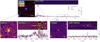 |
Fig. 1. The available photometric and spectroscopic dataset of LAE-11. (upper) A composite image of LAE-11 consisting of the NB926, F125W and F356W photometry, the 2D and 1D NIRSpec/PRISM spectrum of LAE-11 located at z = 6.6405 ± 0.0005. The uncertainty on each pixel of the 1D spectrum is represented with a red line. The vertical dotted lines represent detected emission lines. From left to right: Lyα, Hβ, [OIII] doublet, and Hα. The spectral energy distribution of LAE-11, encompassing photometric data from Subaru/HSC (blue squares), HST/WFC3 (purple circles), and JWST/NIRCam (pink triangles) is shown on top of the 1D NIRSpec spectrum. (lower)NB926 image, 2D and 1D Keck/DEIMOS spectrum of LAE-11 on the left with F356W image, 2D and 1D JWST/NIRCam WFSS spectrum of LAE-11 on the right. The uncertainty on each pixel in both spectra are represented with a red line. The vertical dashed lines mark the position of the Lyα in the DEIMOS spectrum, Hβ and [OIII] doublet emission lines in the NIRCam spectrum. The vertical shaded regions in the DEIMOS spectrum represent the skyline regions. |
Quasar proximity zones trace small regions of highly ionised hydrogen around a luminous quasar, driven by the central active galactic nucleus (AGN; Madau & Pozzetti 2000; Wyithe & Loeb 2004; Eilers et al. 2017; Satyavolu et al. 2023), allowing observations of flux bluewards of Lyα at high-z. As seen in Zheng et al. (2006), Meyer et al. (2022), Wang et al. (2023) and others, high-z quasars, due to their implied large halo masses, are expected to trace overdense regions and protoclusters of star-forming galaxies, potentially increasing the chance of detecting LAEs in their vicinity; however, observational results do not reach a consensus with some quasars lacking an overdense environment (e.g. Bañados et al. 2013; Mazzucchelli et al. 2017; Champagne et al. 2023; Rojas-Ruiz et al. 2024). As such, a high number of LAEs have been found in the proximity zone of the quasar J0910-0414, which was part of the A SPectroscopic survey of biased halos In the Reionization Era (ASPIRE) survey (Wang et al. 2023). One of these galaxies is located at a proper distance of dQSO ∼ 0.3 pMpc from the quasar, designated LAE-11, and displays a double-peaked Lyα emission line (Wang et al. 2024a), whose presence confirms the existence of an ionised region around J0910-0414. In this paper, we present a detail study of LAE-11 using data from Subaru Telescope, Keck Telescope, Hubble Space Telescope (HST), and James Webb Space Telescope (JWST).
The structure of this paper is as follows. In Section 2 we describe the available data for LAE-11, and their respective reductions. In Section 3, we detail the procedure used to calculate the systemic redshift of LAE-11, methods used to extract emission line measurements and the UV properties of the galaxy, and the SED-fitting of the spectro/photometric data available in this study. In Section 4, we present the measurements of the ionising properties of LAE-11, as well as the star formation rate (SFR) measurements. Moreover, we focus on the quasar itself and calculate its opening angle and lifetime. Finally, in Section 5, we discuss the effects of the quasar ionising radiation on the galaxy, and discuss the impact that galaxies similar to LAE-11 had in the EoR. Throughout this work, we use the ΛCDM model Planck18 as presented in Planck Collaboration I (2020) with the following parameters: ΩΛ = 0.69, Ωm = 0.31, and H0 = 67.7 km s−1 Mpc−1. All magnitudes quoted in this work are in the absolute bolometric (AB) system (Oke & Gunn 1983).
2. Data
The quasar J0910-0414 was discovered by Wang et al. (2019) using the data from the DESI Legacy imaging Surveys (Dey et al. 2019), the Pan-STARRS1 Survey (Chambers et al. 2016) and additional infrared imaging data. Candidate selection was followed by spectroscopic observations, where J0910-0414 was observed by Magellan/FIRE (Simcoe et al. 2013) and Gemini/GMOS (Hook et al. 2004). These spectra showcase a strong blueshifted CIV absorption feature, which categorises J0910-0414 as a Broad Absorption Line (BAL) quasar. The redshift of the host galaxy was measured with ALMA to be z = 6.6363 ± 0.0003 using the [CII] line (Wang et al. 2024a). Due to its high supermassive black hole (SMBH) mass of M• = (3.59 ± 0.61)×109 M⊙ measured from its MgII line and UV brightness of MUV = −26.61 (Yang et al. 2021), this quasar was selected as a likely candidate to trace an overdensity of galaxies. The quasar field and consequently LAE-11 were observed with a number of photometric and spectroscopic surveys which we use in this work, described in the following section. The entire available dataset for LAE-11 is summarised in Fig. 1 and measured photometry can be found in Table 1.
2.1. Photometry
2.1.1. Subaru/HSC
The first targeted photometric observations of the field surrounding quasar J0910-0414 were conducted from November 2019 to January 2020 with the Hyper Suprime-Cam (HSC) mounted on the 8.2 m Subaru Telescope (Miyazaki et al. 2018; Komiyama et al. 2018; Kawanomoto et al. 2018; Furusawa et al. 2018). The imaging covered a circular field of view with r ∼ 40′ centred on the quasar (Wang et al. 2024a). The field was observed using two broad band filters, i2 and z, and the narrow band filter NB926 designed to capture the Lyα emission of J0910-0414’s surrounding galaxies across the redshift range 6.494 < zLyα < 6.739. The exposure times were ∼150 minutes, ∼240 minutes, and ∼313 minutes, respectively.
Photometry of LAE-11 obtained with the Subaru/HSC, HST, and JWST.
The detailed data reduction process using the hscPipe 6.7 pipeline (Jurić et al. 2017; Bosch et al. 2018) and LAE selection criteria are described in Wang et al. (2024a), though we provide a brief overview here. First, each individual observation was processed, calibrated, and then combined into a stacked mosaic. Afterwards, the pipeline implements photometric and astrometric calibrations to the stacked mosaics, resulting in a seeing in each mosaic of 0.79″, 0.74″, and 0.56″ with 5σ limiting magnitudes measured in 1 5 diameter apertures of 27.31, 26.27, and 25.71 for filters i2, z, and NB926, respectively. To create a dataset of nearby LAE candidates, Wang et al. (2024a) imposed a colour selection requiring a substantially stronger detection in the narrow band filter compared to the broad band filter. The photometry was then extracted using the hscPipe pipeline. We use the measured magnitudes found in Wang et al. (2024a)
2.1.2. HST
To measure the rest-frame UV emission and spectral energy distribution (SED) of the galaxies clustered around the quasar J0910-0414, we used photometry with high spatial resolution which was obtained using the Wide Field Camera 3 (WFC3; Kimble et al. 2008) on board the HST (Wang et al. 2020, PID 16187; P.I. Feige Wang) on March 10, 2022. The observations utilised four primary orbits and were taken in the near-infrared F125W and F160W bands, centred on the position of the quasar, covering an area of ∼31 arcmin2. The HST imaging was processed, calibrated and drizzled using the DrizzlePac package v3.2.1 (Fruchter et al. 2010) with the reference calibration file hst_0988.pmap. The resulting drizzled and stacked mosaics result in exposure times of 9582.75 s and 10 897.40 s with 5σ limiting magnitudes of 28.26 and 27.98 measured in a 0 4 diameter apertures for filters F125W and F160W, respectively. We extracted the photometry using source-extractor (Bertin & Arnouts 1996).
2.1.3. JWST
We used complementary data obtained with the NIRCam instrument (Rieke et al. 2003) on board the JWST, which were taken as part of the medium-size JWST Cycle 1 programme ASPIRE (PID 2078, P.I. Feige Wang). The survey focused on 25 quasar fields at 6.5 < z < 6.8, including the quasar J0910-0414. The photometric observations were taken in August 2022 with the broad band filters F115W, F200W, and F356W, covering an area of ∼11 arcmin2. This configuration covers the rest-frame optical emission from the quasar and its surrounding galaxies. The NIRCam data were processed using the standard JWST pipeline (Bushouse et al. 2022) v1.8.3 in combination with a custom set of scripts which are detailed in Wang et al. (2023) and Yang et al. (2023). The reference calibration file jwst_1015.pmap was utilised. The resulting exposure times are 1417.254 s, 3779.344 s, and 1417.254 s and 5σ magnitudes of 29.24, 29.68, and 27.82 measured in 0 32 diameter apertures for filters F115W, F200W, and F356W, respectively. A source catalogue was extracted using SourceXtractor++ (Bertin et al. 2020) and the detailed procedure is described in Champagne et al. (2025a).
2.2. Spectroscopy
2.2.1. Keck/DEIMOS
We used optical spectroscopic data provided by the DEep Imaging Multi-Object Spectrograph (DEIMOS) (Faber et al. 2003) mounted on the 10 m Keck-II Telescope, which were obtained as a spectroscopic follow-up of the LAE candidates in the field of J0910-0414 by Wang et al. (2024a). LAE-11 was observed on Feb. 25, 2022, utilising a mask with a ∼1″ slit width, the filter OG550, and the 830G grating (Wang et al. 2024a). The combination of these parameters allows for a spectral dispersion of 0.47 Å/px and a resolving power of R ∼ 4650. The seeing on the night of the observation varied from 0.6″ to 1.5″. Overall, 18 exposures lasting 1200 s each were taken.
We reduced the available spectroscopic data using the Python-based package for semi-automated reduction of astronomical spectra Pypeit v1.15.1 (Prochaska et al. 2020). We followed a standard spectroscopic reduction for Keck/DEIMOS, consisting of flat fielding, wavelength calibration, optimal extraction, and flux calibration for each observation. We carefully modelled the sky lines to correctly reconstruct the underlying spectrum. The normalised residuals of the sky model are presented in Fig. A.1. Afterwards, the 1D and 2D reduced spectral outputs were stacked, resulting in the total exposure time of 6 hours.
2.2.2. JWST/NIRCam WFSS
In addition to imaging survey, the ASPIRE collaboration obtained spectroscopic observations of the targeted 25 quasar fields using NIRCam Wide Field Slitless Spectroscopy (WFSS). These observations were targetting the [OIII] doublet of galaxies in the redshift range of 5.3 < z < 6.5. The full description of the reduction steps is described in detail in Wang et al. (2023), but we provide a brief overview here. The WFSS observations employed grism-R paired with the F356W filter, providing a wavelength coverage spanning 3.1 − 3.9 μm. The detection of LAE-11 fell onto module A of the detector. A primary dithering pattern was employed, using the three-point INTRAMODULEX pattern, with a secondary subpixel dithering pattern 2-POINT-LARGE-WITH-NIRISS. The data were reduced using the same procedure as the NIRCam imaging data. Additionally, a tracing and dispersion model based on the work of Sun et al. (2022) was built to extract the 1D spectra from individual exposures with optimal extraction (Horne 1986). These 1D spectra were stacked with inverse variance weighting as detailed in Wang et al. (2023). However, Wang et al. (2023) note that the offset between the spectral tracing model and the data along the dispersion axis cannot be estimated due to the lack of in-flight wavelength calibration data. As a conservative measure, they propose a constant velocity offset of < 100 km s−1, or Δz < 0.003 for the detected [OIII] emitters. The final spectra have exposure times of 3779.343 s, resolving power of ∼1300–1600 and dispersion of ∼10 Å/px.
2.2.3. JWST/NIRSpec MSA
Finally, we used data from a follow-up observation of J0910-0414 and its protocluster with JWST/NIRSpec MultiObject Spectroscopy (MSA) (Jakobsen et al. 2022), which was conducted in November 2023 (PID 2028; P.I. Feige Wang). The PRISM/CLEAR setup was employed in order to target the rest-frame UV and optical part of the spectrum of galaxies at z ∼ 6.6 surrounding the quasar. The NIRSpec spectrum covers a wavelength range of λ = (6000 − 53 000) Å, or the rest-frame wavelength range of λrest = (785 − 6940) Å. The data was reduced and processed using the standard JWST pipeline v1.13.3 and calibration reference file jwst_1015.pmap was used in the process. The exposure time of the final spectrum is 3939.0 s and has a resolution of R ∼ 100 with an average dispersion of ∼100 Å/px.
3. Methodology
In this section we first describe the methods used to constrain the redshift of LAE-11 and measure the properties of various spectral lines present in the available data. Next, we describe the model and process of SED fitting of the spectrophotometric data. Finally, we measure the UV slope β1550 and absolute UV magnitude MUV of the galaxy, as well as its dust properties.
3.1. Shell modelling of the Lyα emission profile
We use the outflowing shell model (Ahn 2004; Verhamme et al. 2006) to ascertain the physical properties of the scattering gas responsible for the double-peaked Lyα line profile observed in the galaxy. We fitted the Lyα emission line with a mock profile created with the Python package zELDA (Gurung-López et al. 2019, 2022). zELDA uses pre-computed line profiles based on the shell model with the full Monte Carlo radiative transfer code LyaRT (Orsi et al. 2012). The free parameters describe the systemic redshift, zsys, the outflow gas velocity, vout, the neutral hydrogen column density, NHI, the intrinsic equivalent width (EW), EWinj, and the intrinsic width, Winj, of the injected Lyα Gaussian continuum. Due to the negligible dust attenuation in LAE-11 (see Sect. 3.4), we fix the dust optical depth parameter τdust to 0. We sample the entire prior parameter space with 200 000 iterations to constrain the fit with the highest likelihood. The best-fit parameters and their errors are then calculated as the median and 68% confidence interval of the resulting posterior space. The priors, initial and best-fit values for each parameter can be found in Table 2, with the best-fit model presented in Fig. 2. The best-fit shell model showcases a low outflow velocity of  km s−1 with column density of neutral hydrogen of
  . These values are similar to LAEs found at redshifts 2 < z < 3 as reported in Gronke (2017).
Parameters, their priors, and fitted values of the line profile model using pre-computed shell models from zELDA.
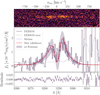 |
Fig. 2. (upper) 2D spectrum showcasing the double-peaked Lyα emission. The shell model fit to the Lyα line profile (middle) and the associated residuals (lower). The dark and light purple lines mark the observed spectrum and its uncertainty. The red line indicates the maximum likelihood model. The dotted blue line shows the median model and the shaded region marks its 1σ posterior. |
We note that the shell model does not account for the apparent absorption at λ ∼ 9280 Å, but rather follows the excess emission present bluewards of the blue peak (λ < 9280 Å). This excess emission allows us to dismiss the nature of the absorption as being due to the sudden increase in the neutrality of the IGM (i.e. the edge of an ionised bubble), as the IGM transmission curve in this scenario scatters any radiation bluewards of Lyα at a certain redshift (see e.g. Mason & Gronke 2020). A possible scenario behind this absorption is a Lyα forest absorber located in the foreground, similar to Lyα forest observations in the spectra of quasars (Lynds 1971).
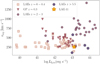 |
Fig. 3. Velocity separation of the Lyα emission profile in relation to its luminosity for z ∼ 0 − 0.4 LAEs (Izotov et al. 2018, 2020, 2021; Izotov et al. 2022, 2024), z ∼ 0.3 GPs (Yang et al. 2017), z ∼ 2 − 3 LAEs (Kulas et al. 2012; Hashimoto et al. 2015; Vanzella et al. 2016), and z ≥ 5.5 LAEs (Hu et al. 2016; Songaila et al. 2018; Bosman et al. 2020; Meyer et al. 2021). LAE-11 is most consistent with local luminous GPs and LAEs. |
3.2. Redshift calibration
We estimated the systemic redshift of LAE-11 by determining the position of the trough of the double-peaked Lyα profile and the redshift of the detected [OIII] doublet. Using the best-fit shell model described in the previous subsection, we measured the redshift of the trough to be  , in line with the measurement presented in Wang et al. (2024a). Next we turn to the JWST NIRCam WFSS spectrum due to its high resolution. We identify a doublet in the 2D and 1D spectra which would correspond to the [OIII] doublet at z ∼ 6.6. We fitted each line with a simple Gaussian and tie the peak separation as dictated by atomic physics (Storey & Zeippen 2000). The [OIII] doublet suggests that LAE-11 is located at z = 6.6372 ± 0.0004. This redshift estimation is in 1σ tension with our Lyα trough calculation even when adopting the conservative calibration redshift offset Δz < 0.003 quoted by Wang et al. (2023). This redshift discrepancy cannot be resolved using the NIRSpec data, as the wavelength resolution is too low to differentiate between the two redshift solutions.
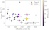 |
Fig. 4. Correlation between [OIII] + Hβ EW0 and the velocity offset of the red Lyα peak as measured by Tang et al. (2024b) for 26 EELGs at z ∼ 2 − 3 (circles). LAE-11 is depicted with a star. The colour of each data point corresponds to the Lyα EW0 of each galaxy. |
Measured emission line properties in the spectra of LAE-11.
We attempted to correct this discrepancy by turning to the other LAEs reported by Wang et al. (2024a) that exhibit an [OIII] doublet and are present in the ASPIRE data. These galaxies are LAE-1 (z[OIII] = 6.537 ± 0.003) and LAE-12 (z[OIII] = 6.632 ± 0.003). Both galaxies showcase a Lyα profile with only one peak. We use the relation found by Verhamme et al. (2018), that ties the full width half maximum (FWHM) of the Lyα line and the offset of the red peak calibrated on a sample of low-z LAEs that are also CIII], Hα, or [OIII] emitters:
 (1)
(1)
We fitted the spectrum of LAE-1 with a spline due to the asymmetric shape of the Lyα line and a Gaussian to the Lyα line of LAE-12 to determine their FWHM. Using Eq. (1), we find that the velocity offset for LAE-1 and LAE-12 is vred = 143.30 ± 66.04 km s−1 and vred = 57.03 ± 61.65 km s−1, respectively. These offsets are then converted to redshifts as z = 6.538 ± 0.002 and z = 6.640 ± 0.002, for LAE-1 and LAE-12. We performed the same procedure using the right peak of LAE-11’s Lyα profile and find z = 6.640 ± 0.002. For LAE-1, we find that this redshift agrees with the value determined using its [OIII] doublet as zLyα − z[OIII] = 0.001; however, for LAE-12 the value is in 2.6σ tension with its [OIII] redshift with zLyα − z[OIII] = 0.008. Meanwhile LAE-11 once again displays 1σ tension of zLyα − z[OIII] = 0.004.
Torralba et al. (2024) showcase an offset in wavelength present in spectra of the same object depending on the NIRCam module used for the observation resulting in a redshift discrepancy of Δz = 0.0016 ± 0.0018. They attribute this offset to a possible astrometry calibration issue or incorrect wavelength solution in the grism data. We checked the modules of our galaxy sample and found that both galaxies with redshift discrepancies fall on module A of the NIRCam detector, while LAE-1 is located on module B (see Fig. A.2). This would imply calibration issues with module A; however, Torralba et al. (2024) find the calibration issues on module B. Moreover, we find a bigger redshift discrepancy in our sample. However, if our data suffers from the same issue, its impact can vary between different observations. This calibration issue could therefore explain the different redshift measurements for Lyα and [O III]. For this reason, we adopt the redshift determined from the trough in the Lyα profile measured from its model as the systemic redshift. However, we discuss the implications on the ionising properties of LAE-11 when taking z[OIII] at face-value in Sect. 5.4.
3.3. Emission line measurements
Due to the high sensitivity of the NIRSpec detector, we were able to detect the continuum emission in the rest-frame UV, and marginally in the rest-frame optical region. To establish the continuum flux density in the UV region of the spectrum, we fitted a simple power law from the Lyα line to the Balmer break. Due to the < 2σ detection of the continuum from the Balmer break to the end of the spectrum, we use the continuum flux density calculated by the SED fitting (see Sect. 3.5).
Afterwards, we modelled and fitted each detected line using a simple Gaussian model and the power-law continuum determined above. We modelled the high-resolution spectrum of the Lyα line with a shell model as described previously. We fitted each Lyα peak with a simple Gaussian to find the red-to-blue peak flux ratio (R/B), which results in R/B ∼ 1.2. When fitting the [O III] doublet, we fitted two Gaussians simultaneously. We tied the peak separation of the two Gaussians; however, we leave the redshift of the two peaks as a free parameter. Additionally, we imposed a uniform prior on the expected flux ratio of the lines from 2.48 to 3.48, centred on 2.98 as dictated by atomic physics (Storey & Zeippen 2000). The uncertainties in the measured properties were determined by perturbing the spectrum by a random draw from a Gaussian distribution whose standard deviation was set to the observed uncertainty of the spectrum. We repeated this process 1000 times, and calculated the 1σ standard deviation for each property. The detected lines, their fluxes, luminosities, and EWs can be found in Table 3.
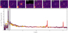 |
Fig. 5. (upper) Imaging of LAE-11 in all available bands across Subaru/HSC, HST/WFC3 and JWST/NIRCam, sorted by wavelength. The dashed white circle corresponds to the aperture used to measure the photometry in each filter. (lower) The observed NIRSpec PRISM spectrum and its 1σ uncertainty are depicted with a dark purple line and purple shaded region, the observed photometry with yellow points and the best-fitting SED model with a red line. The shaded grey region marks the masked Lyα emission line, which was excluded from the fitting process due to the limitations of the model. |
3.4. UV slope, rest-frame UV magnitude, and dust properties
We were able to directly measure the UV slope β1550 of LAE-11, due to the presence of the UV continuum emission in the NIRSpec data. The UV slope is parametrised as a slope of a power-law, following the relation fλ ∝ λβ at λrest = 1550 Å. We measured the UV slope by fitting a power-law to the observed spectrum in 10 wavelength windows, which are defined in Calzetti et al. (1994). To estimate the uncertainty on the measured β1550, we perturbed the observed spectrum 1000 times. Each perturbed spectrum was then fitted within the same region with a power-law. The final uncertainty was calculated as the standard deviation of the distribution of measured β1550 of the 1000 values. The measured UV slope of the NIRSpec spectrum of LAE-11 is  .
.
In addition to the UV slope, we calculated the absolute rest-frame UV magnitude. We used the measured photometric flux from filter F115W, as it is centred on λrest = 1500 Å. We converted the photometric flux to absolute UV magnitude using the luminosity distance of the galaxy. Using this method, we find that the absolute UV magnitude is M . We also measured the absolute UV magnitude using the fit to continuum emission performed in the previous section, which results in M
 . These two values agree within 1σ uncertainty. Since LAE-11 is close to the edge of the F115W field of view (see Fig. 5), we use the MUV calculated from spectroscopy throughout this paper to mitigate any flux loss due to its position. The resulting values can be found in Table 6.
Next, we looked at the dust properties of LAE-11. Using the direct measurement of Hα and Hβ, we calculated the dust attenuation assuming an intrinsic ratio of Hα/Hβ = 2.86 (Osterbrock 1989). For LAE-11 with Hα/Hβ = 2.47 ± 0.42, we measured colour access of  , suggesting a negligible dust attenuation in LAE-11. This is further supported by the dust attenuation obtained from SED fitting (AV < 0.01) described in the following section.
3.5. SED fitting with BAGPIPES
To constrain the properties of the stellar population of the galaxy, we performed SED fitting with the BAGPIPES code (Carnall et al. 2019), using a combination of NIRSpec/PRISM spectroscopy and photometric data. BAGPIPES employs the stellar models introduced in Bruzual & Charlot (2003), that utilise the empirical spectral library MILES (Falcón-Barroso et al. 2011) and Kroupa & Boily (2002) initial mass function (IMF). The models are complemented with additional nebular and continuum emission based on Cloudy models (Ferland et al. 1998; Byler et al. 2017).
The redshift of LAE-11 was fixed to the systemic redshift determined by the trough of the double-peaked Lyα profile to z = 6.6408. We adopted the non-parametric star formation history (SFH) with NSFH bins = 7 bins of Leja et al. (2019), with the first four spanning 0 − 2 Myr, 2 − 4 Myr, 4 − 8 Myr, and 8 − 16 Myr in lookback time to be sensitive to the variation in the recent SFH of the galaxy. The remaining bins were logarithmically spaced in the galaxy’s lookback time from 16 Myr to z = 20 (e.g. Tacchella et al. 2022). Finally, we applied dust attenuation following the dust model introduced in Calzetti et al. (1994) and allow AV to uniformly vary as 0 < AV < 4. For the remaining parameters (stellar mass, M⋆, ionisation parameter, U, metallicity, Z) we used broad uniform priors, listed in Table 4. We masked the wavelength region spanning 1150 Å < λrest < 1450 Å, due to the limitations of the model to reproduce the Lyα region. The resulting best-fit SED template, the predicted and observed photometry, and the NIRSpec spectrum are presented in Fig. 5. The best-fit SFH of LAE-11 is shown in Fig. 6. The best-fit values of the physical parameters are shown in Table 6. The posterior distributions for each parameter can be found in Fig. A.3.
Parameters and priors used for spectrophotometric SED fitting of LAE-11 with BAGPIPES.
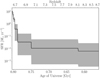 |
Fig. 6. Posterior non-parametric SFH of LAE-11 depicted with a solid black line. The 1σ uncertainty is marked with a shaded grey region. |
4. Results
In this section, we evaluate the ionising properties of LAE-11. First, we calculate the escape fraction of LyC photons using a set of proxies based on empirical relations and multivariate-empirical models. Next, we focus on the ionising photon production efficiency of the galaxy. Afterwards, we measure the SFR of LAE-11. Finally, we investigate the quasar-galaxy geometry and the quasar environment of J0910-0414.
4.1. Escape fraction of Lyman continuum
To investigate the degree of LyC leakage undergoing in LAE-11, we must evaluate fescLyC, the fraction of ionising photons which are able to escape into the IGM. Due to the low IGM attenuation of the Lyα line of high-z galaxies situated in quasar proximity zones, we have a unique opportunity to use the EW and peak separation of Lyα profile to estimate LyC leakage of LAE-11.
First, we measured the escape fraction of LyC photons using the peak separation of the Lyα profile (Verhamme et al. 2017; Izotov et al. 2018; Flury et al. 2022b). The empirical correlation between the velocity separation of the two peaks, Δvsep, and  was estimated using a sample of 56 LyC leaking galaxies at z < 0.4. We determined the peak separation by translating the fitted Lyα emission line model to velocity space and calculating the local maxima (see Section 3.2). We find the velocity separation of the two peaks is Δvsep = 242.71 ± 44.93 km s−1. This value is comparable to local bright GPs and LAEs (see Fig. 3). Using the peak separation and following the relation in Izotov et al. (2018):
 (2)
(2)
we find LyC leakage of  . The reliability of the double-peak Lyα velocity separation as a proxy of LyC leakage has, however, been called into question. Naidu et al. (2022) show that some sources with a high peak separation of vsep > 400 km s−1, such as Ion2, Ion3, Sunburst Arc and others, leak > 20% of their ionising photons. Additionally, numerical simulations by Choustikov et al. (2024) indicate that while it is unlikely to find strong leakers with wide peak separation, they find no real trend between the two quantities. A similar trend is observed in simulations by Giovinazzo et al. (2024) for example, where multiple objects with low peak separation also showcase a low
  . However, it is still unclear whether these results are a product of a simulation bias. For this reason, we use additional estimators of LyC leakage to provide reliable measurements.
Begley et al. (2024) probe the correlation between the escape fraction of Lyα photons  and
and  with a sample of 152 star-forming galaxies (SFGs) at 4 < z < 5. They first find a scaling relation between the EW0(Lyα) and the Lyα escape fraction, which is then found to be in a linear correlation with
  . Following their method, assuming negligible dust attenuation, and using the measured EW(Lyα), we find that for LAE-11 the escape fraction of Lyα photons is
  , and subsequently its LyC leakage is
  . Moreover, we used the measured escape fraction of Lyα photons from the best-fit shell model (Sect. 3.2) of
  , resulting in a LyC escape fraction of
  .
.
Next, we employed the empirical relation between the  and the UV slope β1550 derived by Chisholm et al. (2022), using a selection of 89 SFGs and LyC emitters at z ∼ 0.3:
 (3)
(3)
Using this relation we calculated  . We note that the relation more robustly characterises a population-average escape fractions than an individual scenarios, resulting in the large uncertainty on the calculated
  .
.
Naidu et al. (2020) examine the correlation between the SFR density ΣSFR, and LyC leakage. We used their empirical model:
 (4)
(4)
We used both ΣSFR calculated with LUV and L(Hα) described in Section 4.3. Since we only find the lower limits on ΣSFR > 3.59 (9.44) M⊙ yr−1 kpc−2 for LUV (L(Hα)), we find the lower limits for  using LUV (L(Hα)).
To confirm our estimates of  , we used the recent multivariate diagnostic Cox models developed by Jaskot et al. (2024a,b) to empirically predict fescLyC with a combination of observable properties. These models utilise a survival analysis technique to treat data with upper limits appropriately, and was developed using 50 LyC emitting galaxies at z ∼ 0.3. For LAE-11 we used models and their input parameters:
-
LAE with M1500, E(B − V)UV, and EW0(Lyα);
-
ELG-EW with M1500, log M⋆, E(B − V)UV, and logEW0([O III] + Hβ);
-
R50-β, which uses M1500, log M⋆, β1550, and the UV half-light radius R50, UV.
Using these models, we find  ,
,  , ( > 0.18) for models LAE, ELG-EW, and R50-β, respectively. For R50-β model we only calculated the lower limit of the escape fraction, as the radius RUV of the galaxy is smaller than the point spread function (PSF; see Sect. 4.3). We note that the multivariate models indicate higher uncertainties on the estimated values of the escape fraction. Jaskot et al. (2024b) caution that some galaxies at z ≳ 6 differ from the parameter space covered by the sample of low-z galaxies used to calibrate the model, increasing the uncertainties of the predictions. All the determined
  values and the methods used to calculate them can be found in Table 5.
Estimates of the escape fraction of ionising photons from LAE-11 using indirect empirical relations and multivariate models.
Physical properties of LAE-11 calculated from line and continuum properties, and SED fitting.
We compared the estimated values of  that were determined using the Lyα emission and the ones that used other galaxy properties. We find that both the peak separation and LAE model indicate a higher escape fraction of LyC (≳15%), while the relation by Begley et al. (2024) shows fescLyα < 10% only when using the intrinsic Lyα line. Models and relations focusing on galaxy properties not tied to the Lyα emission line do not show any discrepancy as the
  correlation by Chisholm et al. (2022),
  relations, ELG-EW model and the R50-β model estimate a higher escape fraction of ≳10%. We note, however, that these relations are either only lower limits on the escape fractions or show a high 1σ uncertainty. Comparing these two groups of
  proxies, we find that they do not show a significant scatter among the calculated values, and all indicate that at least ≳5% of LAE-11’s LyC photons are leaking into the surrounding IGM. The agreement between all available indirect tracers indicates that each is viable for determining LyC leakage of high-z galaxies; however, multiple tracers are recommended to constrain its exact value. We discuss the implications of the measured
  in Section 5.3.
4.2. Ionising photon production efficiency
In addition to fescLyC, ionising photon production efficiency ξion needs to be calculated to correctly estimate LAE-11’s ionising output. We calculated ξion of LAE-11 using the Hα and Hβ lines, respectively. We have access to both Hα and Hβ lines, and therefore we checked whether the assumption of Case B recombination scenario is warranted. We find that the ratio of Hα/Hβ = 2.47 ± 0.49, which is in 1σ agreement with Case B scenario of Hα/Hβ = 2.86 (Osterbrock 1989). ξion is defined as
 (5)
(5)
where N(H) is the production rate of ionising photons and LUV, corr is the intrinsic UV luminosity of the galaxy, calculated from MUV. We calculated N(H) both with Hα and Hβ separately, assuming a Case B recombination with the Hα (Hβ) line coefficient of CB = 1.36 × 10⁻¹² (4.79 × 10⁻¹³) erg, electron density ne = 103 cm−3, and electron temperature of Te = 104 K, as N(H) =Lline/CB (Leitherer & Heckman 1995), and negligible dust attenuation. Using this method and the measured range of  from Section 4.1, we find for Hα log(ξion, fesc = 0.09/Hz erg−1) = 25.52 ± 0.06 and
  , while for Hβ we find log(ξion, fesc = 0.09/Hz erg−1) = 25.58 ± 0.07 and
  . All the measured values and the methods used to calculate them can be found in Table 6. For ease of reading, we report the value of log(ξion) using the median
  . For Hα and Hβ respectively, we find
  and
and  . We discuss the implications of the measured ξion in Section 5.3.
4.3. Star formation rate and star formation rate density
We calculated the SFR of LAE-11 using its UV and line properties. We utilised the standard relations found in Kennicutt (1998), that use the Salpeter (1955) IMF, and link the SFR of galaxies to their UV luminosity as
 (6)
(6)
and to the luminosity of the Hα line as
 (7)
(7)
We used the UV magnitude and the Hα line from the NIRSpec data to calculate the SFR of LAE-11, assuming a negligible dust attenuation. Following these relations, we find SFRUV = 5.55 ± 0.65 M⊙ yr−1 and SFRHα = 12.93 ± 1.20 M⊙ yr−1. All SFR values calculated in this work can be found in Table 6. The implications of the measured SFR for LAE-11 are further discussed in Sect. 5.2.
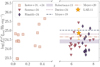 |
Fig. 7. Evolution of the ionising output of galaxies (ξionfescLyC) with redshift. The ionising output required to sustain reionisation determined by Robertson et al. (2013) is depicted with shaded purple region, while the mean ionising output needed to maintain EoR adopted by Davies et al. (2024) is shown with a dotted pink line. The values determined by Meyer et al. (2019, 2020) are shown with a dashed blue and dashdotted pink lines. Low−z SFGs (Izotov et al. 2018, 2024) are shown with pale pink squares, high−z faint LAEs (Saxena et al. 2024) are shown with red triangles, high−z strong Hα emitters (Rinaldi et al. 2024) are shown with purple diamonds, and LAE-11 is depicted with a yellow star. We used the median fescLyC. |
We also evaluated the SFR density of LAE-11 following the definition ΣSFR = SFR/2πRUV2 (e.g. Shibuya et al. 2019; Naidu et al. 2020), where RUV is the UV effective half-light radius. We measured the FWHM of LAE-11 using the value FWHM_IMAGE, that was calculated as a part of photometry extraction run with SourceXtractor, where FWHM is calculated assuming a Gaussian core. Next, we picked and stacked 15 bright visually selected stars. We fitted a 2D Gaussian to the stack in order to calculate the FWHM of the PSF as FWHMPSF = 0.17″. We found that the FWHM of LAE-11 is lower than this value, and therefore we only report an upper limit on the UV radius. Following the approach of Torralba et al. (2024), we calculated the UV radius in physical units as FWHM/2, resulting in RUV < 0.47 kpc. Additionally, we calculated the radius of the galaxy in the Lyα emission present in the NB926 filter, following the same method. LAE-11 is again unresolved and its FWHM is smaller than the PSF of the narrowband data (FWHMPSF = 0.34″). We therefore only report the upper limits on the Lyα radius of RLyα < 1.83 kpc.
Using the upper limit of RUV in turn gives the lower limit for ΣSFR. Using the SFR estimated from the UV luminosity and from Hα, we find ΣSFR > 4.00 M⊙ yr−1 kpc−2 and > 9.44 M⊙ yr−1 kpc−2, respectively. Compared to the sample of galaxies at z ∼ 6 (Shibuya et al. 2015), [OIII] emitters found in the field of COLA1 (Torralba et al. 2024), and strong LyC leakers such as COLA1 (Matthee et al. 2018), Ion2, Ion3 (Vanzella et al. 2016, 2018), and others, LAE-11 belongs in the population with higher ΣSFR based on the lower limits calculated in this work.
4.4. Inferred properties of the quasar J0910-0414
Since we are able to observe the blue peak of the Lyα profile at such a high redshift, LAE-11 is certainly residing within the proximity zone of the quasar. Using the LAEs from Wang et al. (2024a) and [OIII] emitters found by the ASPIRE survey in the vicinity of the quasar whose positions in 3D space can be seen in Fig. 8, we were able to introduce some constraints on the proximity zone of J0910-0414.
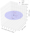 |
Fig. 8. Positions of the LAEs (orange circles) and [OIII] emitters (purple dots) in 3D comoving coordinates with respect to the position of J0910-0414 (blue star). The line-of-sight distance is defined to be negative towards the observer with the quasar positioned at 0 cMpc. RA (Dec) is defined to be negative when the RA (Dec) of the galaxy is smaller than the RA (Dec) of the QSO. The purple plane depicts the declination plane of the quasar. Each galaxy has its position projected onto this plane with a dashed gray line. |
Quasars are known as intrinsically variable sources. The changes in their brightness and thus production of ionising photons affect the surrounding IGM with a time delay, based on its properties and the distance from the quasar, creating a so-called ‘light-echo’ imprint (e.g. Adelberger 2004; Visbal & Croft 2008; Schmidt et al. 2019; Kakiichi et al. 2022). By observing the changes in the IGM located further from the quasar, we are able to determine its lifetime, tQ. The quasar lifetime is defined such that if the light from the recent activity was observed at time t = 0, the quasar actually turned on at a time −tQ in the past (Eilers et al. 2017). Since LAE-11, located ∼0.3 pMpc from the quasar, is residing in the ionised region, it is carrying an imprint of the quasar’s past activity. This allows us to determine the lower limit of the quasar’s lifetime as defined in Bosman et al. (2020):
 (8)
(8)
We measured the line-of-sight proper distance, d∥, and the perpendicular distance along the plane of the sky, d⊥, of LAE-11 from J0910-0414 as d∥ = 0.22 ± 0.01 pMpc and d⊥ = 0.25 pMpc, respectively. Using Eq. (8), we find the lower limit of J0910-0414’s lifetime to be tQ > 3.8 × 10⁵ yr. In Fig. 10, we compare the lifetime of J0910-0414 to other quasars. On the basis of short observed proximity zones along the line-of-sight, some quasars at z ≳ 6 have been identified as being ‘young’ with bright-phase lifetimes tQ < 104 yr (Eilers et al. 2018, 2021). Even though the proximity zone of J0910-0414 is not visible due to its nature as a BAL quasar, the fact that its ionisation field reaches the location of LAE-11 independently demonstrates that it is not a young quasar. Its bright-phase lifetime is more consistent with the mean lifetime of quasars at z < 5 measured from their He II proximity zones (Khrykin et al. 2021; Worseck et al. 2021) and from clustering arguments (e.g. Laurent et al. 2017).
Next, we analysed J0910-0414’s possible opening angles. We assume that the quasar is radiating in a bipolar cone with an opening angle θQ with an ionising photon production rate  . By using the available photometry in the yps1 band and the UV slope β for J0910-0414 from Yang et al. (2021), we integrated over the luminosity density Lν of the quasar as
  . We find that the ionising photon production rate in the observed frame of the quasar is
  s−1. The quasar’s surroundings are unaffected by the photoionisation rate outside of the bipolar cones, while on the inside they are affected by a ionisation field given by photoionisation rate ΓHIQSO:
![Mathematical equation: $$ \begin{aligned} \Gamma _\mathrm{HI} ^\mathrm{QSO} (d_\perp , d_\parallel ) = \frac{-\sigma _{\lambda 912}\beta }{3-\beta }\frac{\dot{N}_\mathrm{ion} ^\mathrm{QSO} [-\Delta t(d_\perp , d_\parallel )]}{4\pi (d_\perp ^2 + d_\parallel ^2)}\mathrm ~s^{-1}, \end{aligned} $$](/articles/aa/full_html/2025/08/aa53469-24/aa53469-24-eq73.gif) (9)
(9)
where σλ912 is the photoionisation cross section at the Lyman Limit (λ = 912 Å), Δt(d⊥, d∥) is the time delay at a distance dQSO2 = d⊥2 + d∥2 from the quasar, d⊥ is the perpendicular separation along the plane of the sky, and d∥2 is the line-of-sight distance from the quasar with a negative sign towards the observer. Due to the tight constraints on the redshifts of both the quasar and LAE-11, we located the galaxy behind the quasar at  away from the observer in an anti-clockwise direction. This position allows us to constrain the minimal opening angle of the quasar θQ, since both the observer and LAE-11 are within the cone. More specifically, the BAL nature of J0910-0414 suggests that we are viewing it at an angle very close to the edge of the ionisation cone (e.g. DiPompeo et al. 2012; Nair & Vivek 2022). Using the 1σ value of LAE-11’s positional angle, the opening angle of the quasar θQ is then constrained to
 (10)
(10)
for the anti-clockwise and clockwise directions as shown in Fig. 9. The only other quasar for which this measurement could be performed, J0836+0054 (Bosman et al. 2020), requires an ionisation opening angle θQ > 21° to illuminate its proximate double-peaked LAE (see also Borisova et al. 2016). For both of these quasars, the ionisation opening angle is therefore much larger than the measured width of quasar radio jets, θQ, radio < 2° (Pushkarev et al. 2017).
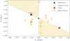 |
Fig. 9. Physical neighbourhood of Q9010 (black circle) surrounded by proximate [OIII] emitters from the ASPIRE survey (yellow stars) and LAEs from Wang et al. (2024a, red stars), and LAE-11 (dark blue star). The parallel distance, d∥, is defined as negative towards the observer. The perpendicular distance, d⊥, is defined as negative if RAgal < RAQSO. We note that LAE-12 is also an [OIII] emitter, and showed with an orange colour. J0910-0414’s ionisation field (yellow shaded yellow region) is depicted anti-clockwise from the observer and depicts the lower limit on its opening angle θQ, assuming a bipolar cone geometry. Since both the observer and the double-peaked LAE must be within this region, we can infer that the lower limit of θQ > 49.17°. |
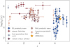 |
Fig. 10. Quasar lifetimes from literature as a function of redshift. Measurements using HI proximity zones along the line of sight are shown with blue squares (Eilers et al. 2018, 2021; Davies et al. 2019, 2020; Andika et al. 2020; Morey et al. 2021), studies using quasar clustering are depicted with red circles (Shen et al. 2007; Shankar et al. 2010; White et al. 2012; Laurent et al. 2017). Measurements inferred from the duty cycle of the quasar host population are shown with grey triangles (Yu & Tremaine 2002; Chen & Gnedin 2018), while those using extends of Lyα nebulae are depicted with purple pentagons (Trainor & Steidel 2013; Cantalupo et al. 2014; Hennawi et al. 2015; Borisova et al. 2016). Furthermore, quasar lifetime estimates calculated from the HeII proximity zones are shown as light brown crosses (Khrykin et al. 2019, 2021; Worseck et al. 2021), and studies using the transverse proximity effect are marked with a pink diamond (Kirkman & Tytler 2008; Keel et al. 2012; Schmidt et al. 2017, 2018; Oppenheimer et al. 2018; Bosman et al. 2020). Our estimation of tQ for J0910-0414 is depicted with a yellow star. Adapted from Eilers et al. (2021). |
We note that the other two LAEs observed in close proximity to J0910-0414 (red and dark orange in Fig. 9) do not show double-peaked Lyα morphologies, but this is not necessarily an indication that they are located outside of the ionisation cone. At z < 3, only roughly ∼1/3 − 1/2 of the LAEs are double-peaked (Kulas et al. 2012; Trainor et al. 2015). Furthermore, their velocity offsets of vred, LAE − 1 = 143.30 ± 66.04 km s−1 and vred, LAE − 12 = 57.03 ± 61.65 km s−1 are comparable to velocity offsets of galaxies found inside ionised regions at similar redshift (e.g. Hayes & Scarlata 2023).
5. Discussion
5.1. Quasar contribution to LAE-11’s Lyα emission
The ionisation field of QSOs can influence the Lyα emission of its nearby LAEs, contributing with a fluorescence-triggered emission. Fluorescence results from the reprocessing of ionised photons from the QSO by the neutral hydrogen gas clouds in the proximate galaxies (e.g. Hogan & Weymann 1987; Cantalupo et al. 2007; Hennawi & Prochaska 2013). This effect is observable either if the LAE is in the foreground, or d ≲ 3.2 pMpc in the background of the quasar (Trainor & Steidel 2013). Since LAE-11 is only ∼0.3 pMpc behind J0910-0414, we calculated the quasar’s contribution to its Lyα luminosity.
Following the method of Bosman et al. (2020), we defined the fluorescent Lyα luminosity contributed to a system with a cross section σLAE and distance dQSO from the quasar as
 (11)
(11)
where fϕ is the illuminating fraction. Assuming that all fluorescent emission is scattered into the line-of-sight, the illuminating fraction takes on the value fϕ = 1. For the cross section of LAE-11, we assumed a simplified spherical geometry of σLAE − 11 = 4πRLyα2. Finally, we used  calculated in the previous section and find that J0910-0414 contributes < 3% within 3σ uncertainty to the Lyα luminosity of LAE-11.
5.2. Star formation in the quasar environment
Quasars and AGN have been proposed as a likely driver behind quenching of star formation in host and proximate galaxies, as their outflows can prevent gas from cooling and delay the onset of star formation (e.g. Silk & Rees 1998; Kashikawa et al. 2007; Fabian 2012) or even completely expel gas reservoirs in small haloes (Mh ≤ 107 M⊙) located at a distance of 1 pMpc in ≲108 years (Shapiro et al. 2004). Due to LAE-11’s close proximity to J0910-0414, we wished to examine the impact of the quasar’s ionisation field on the star formation of the galaxy.
We began by calculating the UV intensity of the QSO radiation at the location of LAE-11 in the units of J21, where J21 = 1 corresponds to an intensity of 10−21 erg s−1 cm−2 Hz−1 sr−1 at the Lyman limit (LL; λ = 912 Å):
 (12)
(12)
where LLLQSO is the quasar’s luminosity at the Lyman limit and d is the physical distance from the quasar to LAE-11. We again utilised the available photometry in the yps1 band and the UV slope, β, from Yang et al. (2021) to calculate LLLQSO. Following this method, we find that the UV intensity at LAE-11’s location is J21 = 3.19 ± 0.32. Kashikawa et al. (2007) show that star formation is completely suppressed in haloes with Mh ≤ 3 × 10⁹ M⊙ at intensity J21 ≥ 3.
The absence of a Balmer break in the spectrum of LAE-11 points towards an absence of older stellar population. This trend can also be observed in the recovered SFH from the spectrophotometric SED fit (see Fig. 6). We note, however, that Witten et al. (2025) found that a young stellar population of 1/3 of the total stellar mass can effectively suppress the Balmer break in the observed spectra of high-z galaxies. The fact that LAE-11 appears to have formed recently is consistent with a delay in the star formation due to the quasar’s influence, but it is also possible that the galaxy’s recent growth would have occurred even in the quasar’s absence. Indeed, studies of larger samples of galaxies around z > 6 quasars find that the quasar has a negligible impact on their properties (Champagne et al. 2025a,b). Therefore, we can only infer the lower limit on the halo mass following the Kashikawa et al. (2007) model as 3 × 10⁹ M⊙ < Mh.
5.3. LAE-11 as a bursty reionisation-driving galaxy
LAE-11 is a galaxy with a blue UV slope β1550 ( ). Topping et al. (2024) investigated the UV slope of galaxies at high redshift and found a median value of β ∼ −2.3 for 5 < z < 7.3. However, they also find 44 objects with extremely blue UV slopes (β ≤ −2.8), that are best described by density-bound HII regions with fescLyC ∼ 0.5. LAE-11 is comparable to these outliers rather than the average galaxy at these redshifts, indicating a high LyC escape fraction. This is further confirmed by our calculation using the fescLyC − β relation found by Chisholm et al. (2022). The significant escape fraction of LyC photons is further confirmed with a selection of indirect tracers (see Table 5), which all point towards an fescLyC of at least > 5%.
The effective production of ionising photons in LAE-11 (Table 6) is comparable to other blue star-forming galaxies at high-z (e.g. Bouwens et al. 2016; Nakajima et al. 2018; Saxena et al. 2024; Simmonds et al. 2023, 2024; Torralba et al. 2024) as well as Hα emitters (HAEs) at z ∼ 7 − 8 (Rinaldi et al. 2024). Additionally, this value is in line with the ionising photon production efficiency of low-z LyC leakers (e.g. Izotov et al. 2018, 2024). However, log(ξion/Hz erg−1) of LAE-11 is higher than the average value found for faint galaxies at z < 4 (Bouwens et al. 2016), or HAEs at z ∼ 2 − 3 (Chen et al. 2024).
By measuring both the fescLyC and ξion of LAE-11, we investigate its total ionising output. This results in  , using the median measured escape of ionising photons. Compared to low-z SFGs, high-z faint LAEs and high-z HAEs, LAE-11 is compatible with the galaxies with effective ionising output (see Fig. 7). Additionally, the usually assumed ionising output of galaxies required to maintain the reionisation of the Universe is log(fescLyCξion/Hz erg−1) = 24.3 − 24.6 (Robertson et al. 2013), 25.01 (Meyer et al. 2019), 24.64 (Meyer et al. 2020) or 24.8 (Davies et al. 2024). These values are lower or comparable to LAE-11’s ionising output. LAE-11 could therefore be a prototypical galaxy with a significant contribution to the ionising budget near the end of the EoR.
The blue UV slope, and an absence of a Balmer break possibly point towards a very young stellar population of the galaxy. The SFR of LAE-11 estimated using the UV emission is lower compared to the one diagnosed via the Hα line with SFRHα/SFRUV = 2.33 ± 0.35. While the nebular emission of Hα traces the formation of the most massive O and B stars with lifetimes of a few million years, the UV emission arises from a wider mass range of the same stellar population measuring timescales of 100 Myr (e.g. Lee et al. 2009). Therefore, the difference in these two tracers might indicate that the galaxy is undergoing a burst of star formation at the time of the observation (e.g. Glazebrook et al. 1999; Sullivan et al. 2000; Domínguez et al. 2015; Emami et al. 2019; Asada et al. 2024). This is further supported by the SFH extracted by SED fitting (Fig. 6).
Reionisation-era galaxies are characterised by extreme [OIII] and Hβ emission, with equivalent widths ranging from 300 Å to 3000 Å (e.g. Endsley et al. 2021, 2023), as expected in galaxies with young stellar populations and low metallicity (e.g. Labbé et al. 2013; De Barros et al. 2019). LAE-11 meets all of these conditions, with EW0([OIII] + Hβ) = 1844 ± 193 Å and log Z/Z⊙ = −0.86 ± 0.03. Furthermore, the high equivalent widths of Lyα, [OIII] and Hβ in the spectra of LAE-11 are comparable to the most extreme EELGs at z ∼ 2 − 3 identified by Tang et al. (2024b) (see Fig. 4).
5.4. Alternative interpretations of LAE-11 at z[OIII]
In this subsection we interpret the ionising properties of LAE-11 when the z[OIII] is taken at face-value. At this redshift, the expected Lyα emission line falls on the left peak of LAE-11’s Lyα profile. The velocity offset of the left peak from the systemic redshift in this scenario falls to vleft = 4.80 ± 24.27 km s−1 and the velocity offset of the right peak is vright = 260.75 ± 24.44 km s−1. A small sample of galaxies with a similar profile (red-dominated with blue peak situated at systemic redshift) were found at lower redshift by Kulas et al. (2012), Trainor et al. (2015) and Vitte et al. (2025). These works suggest that the origin of the double peak in this case arises from processes other than radiative transfer of Lyα photons. Since LAE-11 is a compact source and neither of the peaks is spatially offset from the other in the 2D spectra, we discard the possibility of a satellite source or a merger contaminating our data.
Barring this scenario, the most likely interpretation of the profile would then position the apparent left peak into the centre position of a triple-peaked intrinsic line profile. In this case, the central peak corresponds to Lyα emission which escapes without scattering through holes in the neutral interstellar medium (ISM), while the other two peaks arise due to Lyα photon scattering. In order to see this peak, the IGM around LAE-11 must still be ionised to a high degree. This interpretation is supported by the weak detection of transmission in the spectrum at vsep ∼ −400 km s−1 at ≲2σ, which could be interpreted as the third Lyα line peak (see Fig. 2). Since the left peak would act as the central peak of the line, and is observed, there is an ionised channel in the ISM allowing a 100% leakage of LyC photons from the galaxy (e.g. Zackrisson et al. 2013). However, this result of fescLyC = 100%, would indicate that the ionising photon production efficiency ξion approaches infinity as indicated by Eq. (5), since no Balmer emission lines are expected in this scenario. We also remind the reader of the discussion in Section 3.2, where discrepancies are identified between the Lyα and [O III] redshifts not only for LAE-11 but also for another galaxy which similarly falls on module A of the NIRCam observations.
A final alternative interpretation of the line shape, if the z[OIII] is taken at face value, could be the presence of a neutral hydrogen gas clump in the vicinity of the galaxy. This clump would be responsible for the trough feature in the line profile, which in this scenario has a velocity offset of vtrough = 125.25 ± 22.06 km s−1. This gas with neutral hydrogen column density of  would therefore be falling into the galaxy. Since the double-peak in this scenario would not result from Lyα radiative transfer, the peak separation could not be used for LyC leakage calculation and only other proxies would have to be utilised. However, even in this scenario, LAE-11 would still be required to reside in an ionised IGM as the Lyα emission line would still be highly transmissive at the systemic velocity.
6. Summary
We present an analysis of a double-peaked Lyα emitter in the proximity of quasar J0910-0414 at  discovered in a search for a protocluster anchored by a high-z quasar by Wang et al. (2024a). The detection of the blue peak implies that the galaxy is located within the ionising radiation of the quasar’s proximity zone. We utilise a combination of ground based high-resolution Keck/DEIMOS spectroscopy, JWST WFSS spectroscopy, low-resolution NIRSpec MSA spectroscopy, as well as photometric data spanning the UV to optical wavelengths to characterise the physical parameters and ionising output of the galaxy. Moreover, we use our findings to introduce constraints on the properties of the central quasar. Our key findings are summarised as follows:
-
LAE-11 displays a narrow double-peaked Lyα emission profile with a velocity separation of Δvsep = 242.71 ± 44.93 km/s. The peak separation is comparable to luminous low-z LAEs and GPs, while high-z double-peaked LAEs (Hu et al. 2016; Songaila et al. 2018; Bosman et al. 2020; Meyer et al. 2021) tend to represent the brightest sources with wider peak separation.
-
LAE-11 is a fairly bright UV galaxy (M
 ) with a moderately steep UV slope (
 ). Analysing the direct imaging of LAE-11 reveals a very compact structure of RUV < 0.47 kpc. Using the Balmer decrement, indirect tracers, and SED fitting, we find that LAE-11 is a very dust-poor system. The spectrophotometric fit furthermore characterises the galaxy as low mass (
 ) with low metallicity (log(Z/Z⊙) = − 0.86 ± 0.03). We are also able to report on the SFR of the galaxy determined both by the UV continuum and the Hα line to be SFRUV = 5.55 ± 0.65 M⊙ yr−1 and SFRHα = 12.93 ± 1.20 M⊙ yr−1.
 -
Utilising a number of indirect tracers and multivariate models, we evaluate the escape fraction of ionising photons
 . We find that all tracers point towards an escape fraction of at least ≥5%, with all diagnostics pointing towards an escape fraction of
  . Furthermore, we calculate the ionising photon production efficiency using a median
  to be
to be  (
( ) using the Hα (Hβ) emission line detected in the NIRSpec spectrum. The total ionising output of the galaxy is therefore
  . This is higher or comparable to the canonical value commonly used for galaxies in order to maintain the EoR (Robertson et al. 2013; Meyer et al. 2019, 2020; Davies et al. 2024). LAE-11 therefore belongs to the population of galaxies which inject a significant amount of ionising radiation into the IGM in the early Universe.
 -
The star formation in LAE-11 has not been extinguished despite the quasar-induced ionising intensity of J21 = 3.19 ± 0.32. Conversely it is undergoing an active star burst at the time of the observation. Therefore, the burst in SFR and the possible lack of older stellar population points towards a recent formation of the galaxy. This is consistent with a delayed SFR due to QSO influence; however, studies of larger samples of of galaxies around z > 6 quasars indicate that their impact on surrounding galaxies is insignificant (Champagne et al. 2025a,b). Following the model presented in Kashikawa et al. (2007) implies that the mass of its dark matter halo is 3 × 10⁹ M⊙ < Mh.
-
Finally, we constrain the opening angle and lifetime of the central quasar J0910-0414. By constraining the location of LAE-11, we find the lower limit on the quasar’s opening angle to be θQ > 49.17° and the lower limit on the quasar lifetime to be tQ > 3.8 × 10⁵ years.
Acknowledgments
KP and SEIB are supported by the Deutsche Forschungsgemeinschaft (DFG) under Emmy Noether grant number BO 5771/1-1. Data presented herein were obtained at Keck Observatory, which is a private 501(c)3 non-profit organization operated as a scientific partnership among the California Institute of Technology, the University of California, and the National Aeronautics and Space Administration. The Observatory was made possible by the generous financial support of the W. M. Keck Foundation. This research is furthermore based in part on data collected at the Subaru Telescope, which is operated by the National Astronomical Observatory of Japan. The authors wish to recognize and acknowledge the very significant cultural role and reverence that the summit of Maunakea has always had within the Native Hawaiian community. We are most fortunate to have the opportunity to conduct observations from this mountain. Moreover, this research is based on observations made with the NASA/ESA Hubble Space Telescope obtained from the Space Telescope Science Institute, which is operated by the Association of Universities for Research in Astronomy, Inc., under NASA contract NAS 5–26555. These observations are associated with programme #16187. This work is also based in part on observations made with the NASA/ESA/CSA James Webb Space Telescope. The data were obtained from the Mikulski Archive for Space Telescopes at the Space Telescope Science Institute, which is operated by the Association of Universities for Research in Astronomy, Inc., under NASA contract NAS 5-03127 for JWST. These observations are associated with programme #2078.
References
- Adelberger, K. L. 2004, ApJ, 612, 706 [Google Scholar]
- Ahn, S.-H. 2004, ApJ, 601, L25 [NASA ADS] [CrossRef] [Google Scholar]
- Andika, I. T., Jahnke, K., Onoue, M., et al. 2020, ApJ, 903, 34 [Google Scholar]
- Asada, Y., Sawicki, M., Abraham, R., et al. 2024, MNRAS, 527, 11372 [Google Scholar]
- Atek, H., Labbé, I., Furtak, L. J., et al. 2024, Nature, 626, 975 [NASA ADS] [CrossRef] [Google Scholar]
- Bañados, E., Venemans, B., Walter, F., et al. 2013, ApJ, 773, 178 [CrossRef] [Google Scholar]
- Begley, R., Cullen, F., McLure, R. J., et al. 2024, MNRAS, 527, 4040 [Google Scholar]
- Bertin, E., & Arnouts, S. 1996, A&AS, 117, 393 [NASA ADS] [CrossRef] [EDP Sciences] [Google Scholar]
- Bertin, E., Schefer, M., Apostolakos, N., et al. 2020, in Astronomical Data Analysis Software and Systems XXIX, eds. R. Pizzo, E. R. Deul, J. D. Mol, J. de Plaa, & H. Verkouter, ASP Conf. Ser., 527, 461 [NASA ADS] [Google Scholar]
- Borisova, E., Lilly, S. J., Cantalupo, S., et al. 2016, ApJ, 830, 120 [Google Scholar]
- Bosch, J., Armstrong, R., & Bickerton, S. 2018, PASJ, 70, S5 [Google Scholar]
- Bosman, S. E. I., Fan, X., Jiang, L., et al. 2018, MNRAS, 479, 1055 [Google Scholar]
- Bosman, S. E. I., Kakiichi, K., Meyer, R. A., et al. 2020, ApJ, 896, 49 [Google Scholar]
- Bosman, S. E. I., Davies, F. B., Becker, G. D., et al. 2022, MNRAS, 514, 55 [NASA ADS] [CrossRef] [Google Scholar]
- Bouwens, R. J., Smit, R., Labbé, I., et al. 2016, ApJ, 831, 176 [Google Scholar]
- Bruzual, G., & Charlot, S. 2003, MNRAS, 344, 1000 [NASA ADS] [CrossRef] [Google Scholar]
- Bushouse, H., Eisenhamer, J., Dencheva, N., et al. 2022, https://doi.org/10.5281/zenodo.7325378 [Google Scholar]
- Byler, N., Dalcanton, J. J., Conroy, C., & Johnson, B. D. 2017, ApJ, 840, 44 [Google Scholar]
- Calzetti, D., Kinney, A. L., & Storchi-Bergmann, T. 1994, ApJ, 429, 582 [Google Scholar]
- Cantalupo, S., Lilly, S. J., & Porciani, C. 2007, ApJ, 657, 135 [NASA ADS] [CrossRef] [Google Scholar]
- Cantalupo, S., Arrigoni-Battaia, F., Prochaska, J. X., Hennawi, J. F., & Madau, P. 2014, Nature, 506, 63 [Google Scholar]
- Carnall, A. C., McLure, R. J., Dunlop, J. S., et al. 2019, MNRAS, 490, 417 [Google Scholar]
- Chambers, K. C., Magnier, E. A., Metcalfe, N., et al. 2016, ArXiv e-prints [arXiv:1612.05560] [Google Scholar]
- Champagne, J. B., Casey, C. M., Finkelstein, S. L., et al. 2023, ApJ, 952, 99 [NASA ADS] [CrossRef] [Google Scholar]
- Champagne, J. B., Wang, F., Yang, J., et al. 2025a, ApJ, 981, 114 [Google Scholar]
- Champagne, J. B., Wang, F., Zhang, H., et al. 2025b, ApJ, 981, 113 [Google Scholar]
- Chen, H., & Gnedin, N. Y. 2018, ApJ, 868, 126 [Google Scholar]
- Chen, N., Motohara, K., Spitler, L., Nakajima, K., & Terao, Y. 2024, ApJ, 968, 32 [Google Scholar]
- Chisholm, J., Saldana-Lopez, A., Flury, S., et al. 2022, MNRAS, 517, 5104 [CrossRef] [Google Scholar]
- Choustikov, N., Katz, H., Saxena, A., et al. 2024, MNRAS, 529, 3751 [NASA ADS] [CrossRef] [Google Scholar]
- Davies, F. B., Hennawi, J. F., & Eilers, A.-C. 2019, ApJ, 884, L19 [Google Scholar]
- Davies, F. B., Wang, F., Eilers, A.-C., & Hennawi, J. F. 2020, ApJ, 904, L32 [NASA ADS] [CrossRef] [Google Scholar]
- Davies, F. B., Bosman, S. E. I., & Furlanetto, S. R. 2024, ArXiv e-prints [arXiv:2406.18186] [Google Scholar]
- Dayal, P., Volonteri, M., Choudhury, T. R., et al. 2020, MNRAS, 495, 3065 [Google Scholar]
- De Barros, S., Oesch, P. A., Labbé, I., et al. 2019, MNRAS, 489, 2355 [NASA ADS] [CrossRef] [Google Scholar]
- Dey, A., Schlegel, D. J., Lang, D., et al. 2019, AJ, 157, 168 [Google Scholar]
- Dijkstra, M. 2014, PASA, 31, e040 [Google Scholar]
- Dijkstra, M., Mesinger, A., & Wyithe, J. S. B. 2011, MNRAS, 414, 2139 [NASA ADS] [CrossRef] [Google Scholar]
- DiPompeo, M. A., Brotherton, M. S., & De Breuck, C. 2012, ApJ, 752, 6 [NASA ADS] [CrossRef] [Google Scholar]
- Domínguez, A., Siana, B., Brooks, A. M., et al. 2015, MNRAS, 451, 839 [CrossRef] [Google Scholar]
- Eilers, A.-C., Davies, F. B., Hennawi, J. F., et al. 2017, ApJ, 840, 24 [NASA ADS] [CrossRef] [Google Scholar]
- Eilers, A.-C., Hennawi, J. F., & Davies, F. B. 2018, ApJ, 867, 30 [Google Scholar]
- Eilers, A.-C., Hennawi, J. F., Davies, F. B., & Simcoe, R. A. 2021, ApJ, 917, 38 [NASA ADS] [CrossRef] [Google Scholar]
- Emami, N., Siana, B., Weisz, D. R., et al. 2019, ApJ, 881, 71 [NASA ADS] [CrossRef] [Google Scholar]
- Endsley, R., Stark, D. P., Chevallard, J., & Charlot, S. 2021, MNRAS, 500, 5229 [Google Scholar]
- Endsley, R., Stark, D. P., Whitler, L., et al. 2023, MNRAS, 524, 2312 [NASA ADS] [CrossRef] [Google Scholar]
- Faber, S. M., Phillips, A. C., Kibrick, R. I., et al. 2003, in Instrument Design and Performance for Optical/Infrared Ground-based Telescopes, eds. M. Iye, & A. F. M. Moorwood, SPIE Conf. Ser., 4841, 1657 [Google Scholar]
- Fabian, A. C. 2012, ARA&A, 50, 455 [Google Scholar]
- Falcón-Barroso, J., Sánchez-Blázquez, P., Vazdekis, A., et al. 2011, A&A, 532, A95 [Google Scholar]
- Ferland, G. J., Korista, K. T., Verner, D. A., et al. 1998, PASP, 110, 761 [Google Scholar]
- Finkelstein, S. L., D’Aloisio, A., Paardekooper, J.-P., et al. 2019, ApJ, 879, 36 [Google Scholar]
- Flury, S. R., Jaskot, A. E., Ferguson, H. C., et al. 2022a, ApJS, 260, 1 [NASA ADS] [CrossRef] [Google Scholar]
- Flury, S. R., Jaskot, A. E., Ferguson, H. C., et al. 2022b, ApJ, 930, 126 [NASA ADS] [CrossRef] [Google Scholar]
- Fruchter, A. S., Hack, W., Dencheva, N., et al. 2010, 2010 Space Telescope Science Institute Calibration Workshop, 382 [Google Scholar]
- Furusawa, H., Koike, M., Takata, T., et al. 2018, PASJ, 70, S3 [Google Scholar]
- Gaikwad, P., Haehnelt, M. G., Davies, F. B., et al. 2023, MNRAS, 525, 4093 [NASA ADS] [CrossRef] [Google Scholar]
- Giovinazzo, E., Trebitsch, M., Mauerhofer, V., Dayal, P., & Oesch, P. A. 2024, A&A, 688, A122 [NASA ADS] [CrossRef] [EDP Sciences] [Google Scholar]
- Glazebrook, K., Blake, C., Economou, F., Lilly, S., & Colless, M. 1999, MNRAS, 306, 843 [NASA ADS] [CrossRef] [Google Scholar]
- Gronke, M. 2017, A&A, 608, A139 [NASA ADS] [CrossRef] [EDP Sciences] [Google Scholar]
- Gurung-López, S., Orsi, Á. A., & Bonoli, S. 2019, MNRAS, 490, 733 [CrossRef] [Google Scholar]
- Gurung-López, S., Gronke, M., Saito, S., Bonoli, S., & Orsi, Á. A. 2022, MNRAS, 510, 4525 [NASA ADS] [CrossRef] [Google Scholar]
- Hashimoto, T., Verhamme, A., Ouchi, M., et al. 2015, ApJ, 812, 157 [Google Scholar]
- Hayes, M. J., & Scarlata, C. 2023, ApJ, 954, L14 [NASA ADS] [CrossRef] [Google Scholar]
- Hennawi, J. F., & Prochaska, J. X. 2013, ApJ, 766, 58 [NASA ADS] [CrossRef] [Google Scholar]
- Hennawi, J. F., Prochaska, J. X., Cantalupo, S., & Arrigoni-Battaia, F. 2015, Science, 348, 779 [Google Scholar]
- Hogan, C. J., & Weymann, R. J. 1987, MNRAS, 225, 1P [Google Scholar]
- Hook, I. M., Jørgensen, I., Allington-Smith, J. R., et al. 2004, PASP, 116, 425 [NASA ADS] [CrossRef] [Google Scholar]
- Horne, K. 1986, PASP, 98, 609 [Google Scholar]
- Hu, E. M., Cowie, L. L., Songaila, A., et al. 2016, ApJ, 825, L7 [Google Scholar]
- Inoue, A. K., Shimizu, I., Iwata, I., & Tanaka, M. 2014, MNRAS, 442, 1805 [NASA ADS] [CrossRef] [Google Scholar]
- Izotov, Y. I., Worseck, G., Schaerer, D., et al. 2018, MNRAS, 478, 4851 [Google Scholar]
- Izotov, Y. I., Schaerer, D., Worseck, G., et al. 2020, MNRAS, 491, 468 [NASA ADS] [CrossRef] [Google Scholar]
- Izotov, Y. I., Worseck, G., Schaerer, D., et al. 2021, MNRAS, 503, 1734 [NASA ADS] [CrossRef] [Google Scholar]
- Izotov, Y. I., Chisholm, J., Worseck, G., et al. 2022, MNRAS, 515, 2864 [NASA ADS] [CrossRef] [Google Scholar]
- Izotov, Y. I., Thuan, T. X., Guseva, N. G., et al. 2024, MNRAS, 527, 281 [Google Scholar]
- Jakobsen, P., Ferruit, P., Alves de Oliveira, C., et al. 2022, A&A, 661, A80 [NASA ADS] [CrossRef] [EDP Sciences] [Google Scholar]
- Jaskot, A. E., Dowd, T., Oey, M. S., Scarlata, C., & McKinney, J. 2019, ApJ, 885, 96 [Google Scholar]
- Jaskot, A. E., Silveyra, A. C., Plantinga, A., et al. 2024a, ApJ, 972, 92 [NASA ADS] [CrossRef] [Google Scholar]
- Jaskot, A. E., Silveyra, A. C., Plantinga, A., et al. 2024b, ApJ, 973, 111 [NASA ADS] [CrossRef] [Google Scholar]
- Jurić, M., Kantor, J., Lim, K. T., & Lupton, 2017, in Astronomical Data Analysis Software and Systems XXV, eds. N. P. F. Lorente, K. Shortridge, & R. Wayth, ASP Conf. Ser., 512, 279 [Google Scholar]
- Kakiichi, K., & Gronke, M. 2021, ApJ, 908, 30 [CrossRef] [Google Scholar]
- Kakiichi, K., Schmidt, T., & Hennawi, J. 2022, MNRAS, 516, 582 [Google Scholar]
- Kashikawa, N., Kitayama, T., Doi, M., et al. 2007, ApJ, 663, 765 [NASA ADS] [CrossRef] [Google Scholar]
- Katz, H., Garel, T., Rosdahl, J., et al. 2022, MNRAS, 515, 4265 [NASA ADS] [CrossRef] [Google Scholar]
- Kawanomoto, S., Uraguchi, F., Komiyama, Y., et al. 2018, PASJ, 70, 66 [Google Scholar]
- Keel, W. C., Chojnowski, S. D., Bennert, V. N., et al. 2012, MNRAS, 420, 878 [Google Scholar]
- Kennicutt, R. C., Jr. 1998, ApJ, 498, 541 [Google Scholar]
- Khrykin, I. S., Hennawi, J. F., & Worseck, G. 2019, MNRAS, 484, 3897 [Google Scholar]
- Khrykin, I. S., Hennawi, J. F., Worseck, G., & Davies, F. B. 2021, MNRAS, 505, 649 [CrossRef] [Google Scholar]
- Kimble, R. A., MacKenty, J. W., O’Connell, R. W., & Townsend, J. A. 2008, in Space Telescopes and Instrumentation 2008: Optical, Infrared, and Millimeter, eds. J. M. Oschmann, Jr., M. W. M. de Graauw, & H. A. MacEwen, SPIE Conf. Ser., 7010, 70101E [Google Scholar]
- Kirkman, D., & Tytler, D. 2008, MNRAS, 391, 1457 [Google Scholar]
- Komiyama, Y., Obuchi, Y., Nakaya, H., et al. 2018, PASJ, 70, S2 [Google Scholar]
- Kroupa, P., & Boily, C. M. 2002, MNRAS, 336, 1188 [Google Scholar]
- Kulas, K. R., Shapley, A. E., Kollmeier, J. A., et al. 2012, ApJ, 745, 33 [Google Scholar]
- Kulkarni, G., Keating, L. C., Haehnelt, M. G., et al. 2019, MNRAS, 485, L24 [Google Scholar]
- Labbé, I., Oesch, P. A., Bouwens, R. J., et al. 2013, ApJ, 777, L19 [CrossRef] [Google Scholar]
- Laurent, P., Eftekharzadeh, S., Le Goff, J.-M., et al. 2017, JCAP, 2017, 017 [CrossRef] [Google Scholar]
- Lee, J. C., Gil de Paz, A., Tremonti, C., et al. 2009, ApJ, 706, 599 [NASA ADS] [CrossRef] [Google Scholar]
- Leitherer, C., & Heckman, T. M. 1995, ApJS, 96, 9 [NASA ADS] [CrossRef] [Google Scholar]
- Leja, J., Carnall, A. C., Johnson, B. D., Conroy, C., & Speagle, J. S. 2019, ApJ, 876, 3 [Google Scholar]
- Lynds, R. 1971, ApJ, 164, L73 [NASA ADS] [CrossRef] [Google Scholar]
- Madau, P., & Dickinson, M. 2014, ARA&A, 52, 415 [Google Scholar]
- Madau, P., & Pozzetti, L. 2000, MNRAS, 312, L9 [NASA ADS] [CrossRef] [Google Scholar]
- Mascia, S., Pentericci, L., Calabrò, A., et al. 2024, A&A, 685, A3 [NASA ADS] [CrossRef] [EDP Sciences] [Google Scholar]
- Mason, C. A., & Gronke, M. 2020, MNRAS, 499, 1395 [Google Scholar]
- Mason, C. A., Treu, T., Dijkstra, M., et al. 2018, ApJ, 856, 2 [Google Scholar]
- Matsuda, Y., Yamada, T., Hayashino, T., Yamauchi, R., & Nakamura, Y. 2006, ApJ, 640, L123 [NASA ADS] [CrossRef] [Google Scholar]
- Matthee, J., Sobral, D., Darvish, B., et al. 2017, MNRAS, 472, 772 [Google Scholar]
- Matthee, J., Sobral, D., Gronke, M., et al. 2018, A&A, 619, A136 [NASA ADS] [CrossRef] [EDP Sciences] [Google Scholar]
- Mazzucchelli, C., Bañados, E., Venemans, B. P., et al. 2017, ApJ, 849, 91 [Google Scholar]
- Meyer, R. A., Bosman, S. E. I., Kakiichi, K., & Ellis, R. S. 2019, MNRAS, 483, 19 [NASA ADS] [CrossRef] [Google Scholar]
- Meyer, R. A., Kakiichi, K., Bosman, S. E. I., et al. 2020, MNRAS, 494, 1560 [Google Scholar]
- Meyer, R. A., Laporte, N., Ellis, R. S., Verhamme, A., & Garel, T. 2021, MNRAS, 500, 558 [Google Scholar]
- Meyer, R. A., Decarli, R., Walter, F., et al. 2022, ApJ, 927, 141 [NASA ADS] [CrossRef] [Google Scholar]
- Miyazaki, S., Komiyama, Y., Kawanomoto, S., et al. 2018, PASJ, 70, S1 [NASA ADS] [Google Scholar]
- Morey, K. A., Eilers, A.-C., Davies, F. B., Hennawi, J. F., & Simcoe, R. A. 2021, ApJ, 921, 88 [Google Scholar]
- Naidu, R. P., Tacchella, S., Mason, C. A., et al. 2020, ApJ, 892, 109 [NASA ADS] [CrossRef] [Google Scholar]
- Naidu, R. P., Matthee, J., Oesch, P. A., et al. 2022, MNRAS, 510, 4582 [CrossRef] [Google Scholar]
- Nair, A., & Vivek, M. 2022, MNRAS, 511, 4946 [NASA ADS] [CrossRef] [Google Scholar]
- Nakajima, K., & Ouchi, M. 2014, MNRAS, 442, 900 [Google Scholar]
- Nakajima, K., Fletcher, T., Ellis, R. S., Robertson, B. E., & Iwata, I. 2018, MNRAS, 477, 2098 [NASA ADS] [CrossRef] [Google Scholar]
- Nakane, M., Ouchi, M., Nakajima, K., et al. 2024, ApJ, 967, 28 [NASA ADS] [CrossRef] [Google Scholar]
- Oke, J. B., & Gunn, J. E. 1983, ApJ, 266, 713 [NASA ADS] [CrossRef] [Google Scholar]
- Oppenheimer, B. D., Segers, M., Schaye, J., Richings, A. J., & Crain, R. A. 2018, MNRAS, 474, 4740 [NASA ADS] [CrossRef] [Google Scholar]
- Orlitová, I., Verhamme, A., Henry, A., et al. 2018, A&A, 616, A60 [Google Scholar]
- Orsi, A., Lacey, C. G., & Baugh, C. M. 2012, MNRAS, 425, 87 [NASA ADS] [CrossRef] [Google Scholar]
- Osterbrock, D. E. 1989, Astrophysics of Gaseous Nebulae and Active Galactic Nuclei (University Science Books) [Google Scholar]
- Planck Collaboration I. 2020, A&A, 641, A1 [NASA ADS] [CrossRef] [EDP Sciences] [Google Scholar]
- Prochaska, J., Hennawi, J., Westfall, K., et al. 2020, J. Open Source Softw., 5, 2308 [NASA ADS] [CrossRef] [Google Scholar]
- Pushkarev, A. B., Kovalev, Y. Y., Lister, M. L., & Savolainen, T. 2017, MNRAS, 468, 4992 [Google Scholar]
- Rieke, M. J., Baum, S. A., Beichman, C. A., et al. 2003, in IR Space Telescopes and Instruments, ed. J. C. Mather, SPIE Conf. Ser., 4850, 478 [Google Scholar]
- Rinaldi, P., Caputi, K. I., Iani, E., et al. 2024, ApJ, 969, 12 [NASA ADS] [CrossRef] [Google Scholar]
- Robertson, B. E., Furlanetto, S. R., Schneider, E., et al. 2013, ApJ, 768, 71 [Google Scholar]
- Robertson, B. E., Ellis, R. S., Furlanetto, S. R., & Dunlop, J. S. 2015, ApJ, 802, L19 [Google Scholar]
- Rojas-Ruiz, S., Mazzucchelli, C., Finkelstein, S. L., et al. 2024, ApJ, 967, 27 [CrossRef] [Google Scholar]
- Salpeter, E. E. 1955, ApJ, 121, 161 [Google Scholar]
- Satyavolu, S., Eilers, A.-C., Kulkarni, G., et al. 2023, MNRAS, 522, 4918 [Google Scholar]
- Saxena, A., Bunker, A. J., Jones, G. C., et al. 2024, A&A, 684, A84 [NASA ADS] [CrossRef] [EDP Sciences] [Google Scholar]
- Schmidt, T. M., Worseck, G., Hennawi, J. F., Prochaska, J. X., & Crighton, N. H. M. 2017, ApJ, 847, 81 [NASA ADS] [CrossRef] [Google Scholar]
- Schmidt, T. M., Hennawi, J. F., Worseck, G., et al. 2018, ApJ, 861, 122 [Google Scholar]
- Schmidt, T. M., Hennawi, J. F., Lee, K.-G., et al. 2019, ApJ, 882, 165 [Google Scholar]
- Shankar, F., Weinberg, D. H., & Shen, Y. 2010, MNRAS, 406, 1959 [NASA ADS] [Google Scholar]
- Shapiro, P. R., Iliev, I. T., & Raga, A. C. 2004, MNRAS, 348, 753 [NASA ADS] [CrossRef] [Google Scholar]
- Shen, Y., Strauss, M. A., Oguri, M., et al. 2007, AJ, 133, 2222 [NASA ADS] [CrossRef] [Google Scholar]
- Shibuya, T., Ouchi, M., & Harikane, Y. 2015, ApJS, 219, 15 [Google Scholar]
- Shibuya, T., Ouchi, M., Harikane, Y., et al. 2018, PASJ, 70, S15 [Google Scholar]
- Shibuya, T., Ouchi, M., Harikane, Y., & Nakajima, K. 2019, ApJ, 871, 164 [NASA ADS] [CrossRef] [Google Scholar]
- Silk, J., & Rees, M. J. 1998, A&A, 331, L1 [NASA ADS] [Google Scholar]
- Simcoe, R. A., Burgasser, A. J., Schechter, P. L., et al. 2013, PASP, 125, 270 [NASA ADS] [CrossRef] [Google Scholar]
- Simmonds, C., Tacchella, S., Maseda, M., et al. 2023, MNRAS, 523, 5468 [NASA ADS] [CrossRef] [Google Scholar]
- Simmonds, C., Tacchella, S., Hainline, K., et al. 2024, MNRAS, 527, 6139 [Google Scholar]
- Songaila, A., Hu, E. M., Barger, A. J., et al. 2018, ApJ, 859, 91 [Google Scholar]
- Spina, B., Bosman, S. E. I., Davies, F. B., Gaikwad, P., & Zhu, Y. 2024, A&A, 688, L26 [NASA ADS] [CrossRef] [EDP Sciences] [Google Scholar]
- Storey, P. J., & Zeippen, C. J. 2000, MNRAS, 312, 813 [NASA ADS] [CrossRef] [Google Scholar]
- Sullivan, M., Treyer, M. A., Ellis, R. S., et al. 2000, MNRAS, 312, 442 [NASA ADS] [CrossRef] [Google Scholar]
- Sun, F., Egami, E., Pirzkal, N., et al. 2022, ApJ, 936, L8 [NASA ADS] [CrossRef] [Google Scholar]
- Tacchella, S., Finkelstein, S. L., Bagley, M., et al. 2022, ApJ, 927, 170 [NASA ADS] [CrossRef] [Google Scholar]
- Tang, M., Stark, D. P., Ellis, R. S., et al. 2024a, MNRAS, 531, 2701 [NASA ADS] [CrossRef] [Google Scholar]
- Tang, M., Stark, D. P., Ellis, R. S., et al. 2024b, ApJ, 972, 56 [NASA ADS] [CrossRef] [Google Scholar]
- Topping, M. W., Stark, D. P., Endsley, R., et al. 2024, MNRAS, 529, 4087 [NASA ADS] [CrossRef] [Google Scholar]
- Torralba, A., Matthee, J., Naidu, R. P., et al. 2024, A&A, 689, A44 [NASA ADS] [CrossRef] [EDP Sciences] [Google Scholar]
- Trainor, R., & Steidel, C. C. 2013, ApJ, 775, L3 [Google Scholar]
- Trainor, R. F., Steidel, C. C., Strom, A. L., & Rudie, G. C. 2015, ApJ, 809, 89 [NASA ADS] [CrossRef] [Google Scholar]
- Vanzella, E., De Barros, S., Cupani, G., et al. 2016, ApJ, 821, L27 [Google Scholar]
- Vanzella, E., Nonino, M., Cupani, G., et al. 2018, MNRAS, 476, L15 [Google Scholar]
- Verhamme, A., Schaerer, D., & Maselli, A. 2006, A&A, 460, 397 [NASA ADS] [CrossRef] [EDP Sciences] [Google Scholar]
- Verhamme, A., Orlitová, I., Schaerer, D., & Hayes, M. 2015, A&A, 578, A7 [NASA ADS] [CrossRef] [EDP Sciences] [Google Scholar]
- Verhamme, A., Orlitová, I., Schaerer, D., et al. 2017, A&A, 597, A13 [NASA ADS] [CrossRef] [EDP Sciences] [Google Scholar]
- Verhamme, A., Garel, T., Ventou, E., et al. 2018, MNRAS, 478, L60 [Google Scholar]
- Visbal, E., & Croft, R. A. C. 2008, ApJ, 674, 660 [Google Scholar]
- Vitte, E., Verhamme, A., Hibon, P., et al. 2025, A&A, 694, A100 [NASA ADS] [CrossRef] [EDP Sciences] [Google Scholar]
- Wang, F., Yang, J., Fan, X., et al. 2019, ApJ, 884, 30 [Google Scholar]
- Wang, F., Banados, E., Bian, F., et al. 2020, Mapping A Distant Protocluster Anchored by A Luminous Quasar in the Epoch of Reionization, HST Proposal. Cycle 28, ID. #16187 [Google Scholar]
- Wang, F., Yang, J., Hennawi, J. F., et al. 2023, ApJ, 951, L4 [NASA ADS] [CrossRef] [Google Scholar]
- Wang, F., Yang, J., Hennawi, J. F., et al. 2024a, ApJ, 962, L11 [NASA ADS] [CrossRef] [Google Scholar]
- Wang, F., Yang, J., Fan, X., et al. 2024b, ApJ, 968, 9 [NASA ADS] [CrossRef] [Google Scholar]
- White, M., Myers, A. D., Ross, N. P., et al. 2012, MNRAS, 424, 933 [NASA ADS] [CrossRef] [Google Scholar]
- Witten, C., McClymont, W., Laporte, N., et al. 2025, MNRAS, 537, 112 [Google Scholar]
- Worseck, G., Khrykin, I. S., Hennawi, J. F., Prochaska, J. X., & Farina, E. P. 2021, MNRAS, 505, 5084 [NASA ADS] [CrossRef] [Google Scholar]
- Wyithe, J. S. B., & Loeb, A. 2004, Nature, 427, 815 [Google Scholar]
- Yang, H., Malhotra, S., Gronke, M., et al. 2017, ApJ, 844, 171 [NASA ADS] [CrossRef] [Google Scholar]
- Yang, J., Wang, F., Fan, X., et al. 2021, ApJ, 923, 262 [NASA ADS] [CrossRef] [Google Scholar]
- Yang, J., Wang, F., Fan, X., et al. 2023, ApJ, 951, L5 [NASA ADS] [CrossRef] [Google Scholar]
- Yu, Q., & Tremaine, S. 2002, MNRAS, 335, 965 [NASA ADS] [CrossRef] [Google Scholar]
- Zackrisson, E., Inoue, A. K., & Jensen, H. 2013, ApJ, 777, 39 [NASA ADS] [CrossRef] [Google Scholar]
- Zackrisson, E., Binggeli, C., Finlator, K., et al. 2017, ApJ, 836, 78 [NASA ADS] [CrossRef] [Google Scholar]
- Zheng, W., Overzier, R. A., Bouwens, R. J., et al. 2006, ApJ, 640, 574 [NASA ADS] [CrossRef] [Google Scholar]
Appendix A: Additional figures
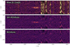 |
Fig. A.1. (upper) The raw coadded 2D spectrum generated by the Pypeit pipeline. (middle) The sky subtraction residuals resulting from the subtraction of the sky model from the raw coadded 2D spectrum. (lower) The final residuals after subtracting both the sky model and the object model, which is used to extract the 1D science spectrum. |
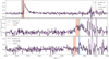 |
Fig. A.2. DEIMOS spectra of the LAEs in our sample with [OIII] spectra from JWST/NIRCam WFSS. LAE-1 (upper), LAE-11 (middle) and LAE-12 (lower) are shown with a purple line, and the skyline regions are marked with a shaded purple region. The dashed blue line represents the redshift of the galaxy as measured from the [OIII] doublet with the shaded blue region representing the conservative calibration redshift offset adopted by Wang et al. (2023), while the dotted orange line corresponds to the redshift calculated using FWHM(Lyα) as seen in Eq. 1 with the shaded orange region representing its measured uncertainty. For LAE-11 the dash-dotted green line and shaded green region represent the systemic redshift measured by the shell model and its uncertainty. |
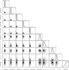 |
Fig. A.3. Corner plots showing the posterior distributions of the free parameters of the SED fit of LAE-11 using BAGPIPES. The contours indicate the 1σ, 2σ, and 3σ posterior of each parameter. The histogram of each parameter is shown on top of the corner plots, with the median shown with a dashed lines indicating the median and 1σ distribution. |
All Tables
Parameters, their priors, and fitted values of the line profile model using pre-computed shell models from zELDA.
Parameters and priors used for spectrophotometric SED fitting of LAE-11 with BAGPIPES.
Estimates of the escape fraction of ionising photons from LAE-11 using indirect empirical relations and multivariate models.
Physical properties of LAE-11 calculated from line and continuum properties, and SED fitting.
All Figures
|
Fig. 1. The available photometric and spectroscopic dataset of LAE-11. (upper) A composite image of LAE-11 consisting of the NB926, F125W and F356W photometry, the 2D and 1D NIRSpec/PRISM spectrum of LAE-11 located at z = 6.6405 ± 0.0005. The uncertainty on each pixel of the 1D spectrum is represented with a red line. The vertical dotted lines represent detected emission lines. From left to right: Lyα, Hβ, [OIII] doublet, and Hα. The spectral energy distribution of LAE-11, encompassing photometric data from Subaru/HSC (blue squares), HST/WFC3 (purple circles), and JWST/NIRCam (pink triangles) is shown on top of the 1D NIRSpec spectrum. (lower)NB926 image, 2D and 1D Keck/DEIMOS spectrum of LAE-11 on the left with F356W image, 2D and 1D JWST/NIRCam WFSS spectrum of LAE-11 on the right. The uncertainty on each pixel in both spectra are represented with a red line. The vertical dashed lines mark the position of the Lyα in the DEIMOS spectrum, Hβ and [OIII] doublet emission lines in the NIRCam spectrum. The vertical shaded regions in the DEIMOS spectrum represent the skyline regions. |
| In the text | |
|
Fig. 2. (upper) 2D spectrum showcasing the double-peaked Lyα emission. The shell model fit to the Lyα line profile (middle) and the associated residuals (lower). The dark and light purple lines mark the observed spectrum and its uncertainty. The red line indicates the maximum likelihood model. The dotted blue line shows the median model and the shaded region marks its 1σ posterior. |
| In the text | |
|
Fig. 3. Velocity separation of the Lyα emission profile in relation to its luminosity for z ∼ 0 − 0.4 LAEs (Izotov et al. 2018, 2020, 2021; Izotov et al. 2022, 2024), z ∼ 0.3 GPs (Yang et al. 2017), z ∼ 2 − 3 LAEs (Kulas et al. 2012; Hashimoto et al. 2015; Vanzella et al. 2016), and z ≥ 5.5 LAEs (Hu et al. 2016; Songaila et al. 2018; Bosman et al. 2020; Meyer et al. 2021). LAE-11 is most consistent with local luminous GPs and LAEs. |
| In the text | |
|
Fig. 4. Correlation between [OIII] + Hβ EW0 and the velocity offset of the red Lyα peak as measured by Tang et al. (2024b) for 26 EELGs at z ∼ 2 − 3 (circles). LAE-11 is depicted with a star. The colour of each data point corresponds to the Lyα EW0 of each galaxy. |
| In the text | |
|
Fig. 5. (upper) Imaging of LAE-11 in all available bands across Subaru/HSC, HST/WFC3 and JWST/NIRCam, sorted by wavelength. The dashed white circle corresponds to the aperture used to measure the photometry in each filter. (lower) The observed NIRSpec PRISM spectrum and its 1σ uncertainty are depicted with a dark purple line and purple shaded region, the observed photometry with yellow points and the best-fitting SED model with a red line. The shaded grey region marks the masked Lyα emission line, which was excluded from the fitting process due to the limitations of the model. |
| In the text | |
|
Fig. 6. Posterior non-parametric SFH of LAE-11 depicted with a solid black line. The 1σ uncertainty is marked with a shaded grey region. |
| In the text | |
|
Fig. 7. Evolution of the ionising output of galaxies (ξionfescLyC) with redshift. The ionising output required to sustain reionisation determined by Robertson et al. (2013) is depicted with shaded purple region, while the mean ionising output needed to maintain EoR adopted by Davies et al. (2024) is shown with a dotted pink line. The values determined by Meyer et al. (2019, 2020) are shown with a dashed blue and dashdotted pink lines. Low−z SFGs (Izotov et al. 2018, 2024) are shown with pale pink squares, high−z faint LAEs (Saxena et al. 2024) are shown with red triangles, high−z strong Hα emitters (Rinaldi et al. 2024) are shown with purple diamonds, and LAE-11 is depicted with a yellow star. We used the median fescLyC. |
| In the text | |
|
Fig. 8. Positions of the LAEs (orange circles) and [OIII] emitters (purple dots) in 3D comoving coordinates with respect to the position of J0910-0414 (blue star). The line-of-sight distance is defined to be negative towards the observer with the quasar positioned at 0 cMpc. RA (Dec) is defined to be negative when the RA (Dec) of the galaxy is smaller than the RA (Dec) of the QSO. The purple plane depicts the declination plane of the quasar. Each galaxy has its position projected onto this plane with a dashed gray line. |
| In the text | |
|
Fig. 9. Physical neighbourhood of Q9010 (black circle) surrounded by proximate [OIII] emitters from the ASPIRE survey (yellow stars) and LAEs from Wang et al. (2024a, red stars), and LAE-11 (dark blue star). The parallel distance, d∥, is defined as negative towards the observer. The perpendicular distance, d⊥, is defined as negative if RAgal < RAQSO. We note that LAE-12 is also an [OIII] emitter, and showed with an orange colour. J0910-0414’s ionisation field (yellow shaded yellow region) is depicted anti-clockwise from the observer and depicts the lower limit on its opening angle θQ, assuming a bipolar cone geometry. Since both the observer and the double-peaked LAE must be within this region, we can infer that the lower limit of θQ > 49.17°. |
| In the text | |
|
Fig. 10. Quasar lifetimes from literature as a function of redshift. Measurements using HI proximity zones along the line of sight are shown with blue squares (Eilers et al. 2018, 2021; Davies et al. 2019, 2020; Andika et al. 2020; Morey et al. 2021), studies using quasar clustering are depicted with red circles (Shen et al. 2007; Shankar et al. 2010; White et al. 2012; Laurent et al. 2017). Measurements inferred from the duty cycle of the quasar host population are shown with grey triangles (Yu & Tremaine 2002; Chen & Gnedin 2018), while those using extends of Lyα nebulae are depicted with purple pentagons (Trainor & Steidel 2013; Cantalupo et al. 2014; Hennawi et al. 2015; Borisova et al. 2016). Furthermore, quasar lifetime estimates calculated from the HeII proximity zones are shown as light brown crosses (Khrykin et al. 2019, 2021; Worseck et al. 2021), and studies using the transverse proximity effect are marked with a pink diamond (Kirkman & Tytler 2008; Keel et al. 2012; Schmidt et al. 2017, 2018; Oppenheimer et al. 2018; Bosman et al. 2020). Our estimation of tQ for J0910-0414 is depicted with a yellow star. Adapted from Eilers et al. (2021). |
| In the text | |
|
Fig. A.1. (upper) The raw coadded 2D spectrum generated by the Pypeit pipeline. (middle) The sky subtraction residuals resulting from the subtraction of the sky model from the raw coadded 2D spectrum. (lower) The final residuals after subtracting both the sky model and the object model, which is used to extract the 1D science spectrum. |
| In the text | |
|
Fig. A.2. DEIMOS spectra of the LAEs in our sample with [OIII] spectra from JWST/NIRCam WFSS. LAE-1 (upper), LAE-11 (middle) and LAE-12 (lower) are shown with a purple line, and the skyline regions are marked with a shaded purple region. The dashed blue line represents the redshift of the galaxy as measured from the [OIII] doublet with the shaded blue region representing the conservative calibration redshift offset adopted by Wang et al. (2023), while the dotted orange line corresponds to the redshift calculated using FWHM(Lyα) as seen in Eq. 1 with the shaded orange region representing its measured uncertainty. For LAE-11 the dash-dotted green line and shaded green region represent the systemic redshift measured by the shell model and its uncertainty. |
| In the text | |
|
Fig. A.3. Corner plots showing the posterior distributions of the free parameters of the SED fit of LAE-11 using BAGPIPES. The contours indicate the 1σ, 2σ, and 3σ posterior of each parameter. The histogram of each parameter is shown on top of the corner plots, with the median shown with a dashed lines indicating the median and 1σ distribution. |
| In the text | |
Current usage metrics show cumulative count of Article Views (full-text article views including HTML views, PDF and ePub downloads, according to the available data) and Abstracts Views on Vision4Press platform.
Data correspond to usage on the plateform after 2015. The current usage metrics is available 48-96 hours after online publication and is updated daily on week days.
Initial download of the metrics may take a while.