| Issue |
A&A
Volume 700, August 2025
|
|
|---|---|---|
| Article Number | A34 | |
| Number of page(s) | 27 | |
| Section | Cosmology (including clusters of galaxies) | |
| DOI | https://doi.org/10.1051/0004-6361/202554107 | |
| Published online | 31 July 2025 | |
Weak lensing mass-richness relation of redMaPPer clusters in LSST DESC DC2 simulations
1
Université Paris-Saclay, CEA, IRFU, 91191 Gif-sur-Yvette, France
2
Université Grenoble Alpes, CNRS, IN2P3, LPSC, 38000 Grenoble, France
3
Kavli Institute for Cosmological Physics, University of Chicago, Chicago, IL 60637, USA
4
Université Paris Cité, CNRS, IN2P3, APC, 75013 Paris, France
5
Italian National Institute of AstroPhysics, Osservatorio Astronomico di Trieste, Italy
6
Université de Savoie, CNRS, IN2P3, LAPP, Annecy-le-Vieux, France
7
Department of Physics, University of Michigan, Ann Arbor, MI 48109, USA
8
Leinweber Center of Theoretical Physics, University of Michigan, Ann Arbor, MI 48109, USA
9
Department of Statistics and Data Sciences, The University of Texas at Austin, TX 78712, USA
10
The NSF-Simons AI Institute for Cosmic Origins, University of Texas at Austin, Austin, TX 78712, USA
11
HEP Division, Argonne National Laboratory, 9700 S. Cass Ave., Lemont, IL 60439, USA
12
Université Paris-Saclay, Université Paris Cité, CEA, CNRS, AIM, 91191 Gif-sur-Yvette, France
13
School of Mathematics, Statistics and Physics, Newcastle University, Newcastle upon Tyne NE17RU, UK
14
High Energy Physics Division, Argonne National Laboratory, Lemont, IL 60439, USA
15
Kavli Institute for Particle Astrophysics & Cosmology, PO Box 2450 Stanford University, Stanford, CA 94305, USA
16
SLAC National Accelerator Laboratory, Menlo Park, CA 94025, USA
17
Department of Physics and Astronomy, University of California, One Shields Avenue, Davis, CA 95616, USA
⋆ Corresponding author: This email address is being protected from spambots. You need JavaScript enabled to view it.
Received:
11
February
2025
Accepted:
8
June
2025
Abstract
Context. Cluster scaling relations are key ingredients in cluster abundance-based cosmological studies. In optical cluster cosmology, where clusters are detected through their richness, cluster-weak gravitational lensing has proven to be a powerful tool to constrain the cluster mass-richness relation. This work is conducted as part of the Dark Energy Science Collaboration (DESC), which aims to analyze the Legacy Survey of Space and Time (LSST) of the Vera C. Rubin Observatory, starting in 2026.
Aims. Cluster properties inferred from weak lensing, such as mass, suffer from several sources of bias. In this paper, we aim to test the impact of modeling choices and observational systematics in cluster lensing on the inference of the mass-richness relation.
Methods. We constrained the mass-richness relation of 3600 clusters detected by the redMaPPer algorithm in the cosmoDC2 extragalactic mock catalog of the LSST DESC DC2 simulation, covering 440 deg2, using number count measurements and either stacked weak lensing profiles or mean cluster masses in several intervals of richness (20 ≤ λ ≤ 200) and redshift (0.2 ≤ z ≤ 1).
Results. We provide the first constraints on the redMaPPer cluster mass-richness relation detected in cosmoDC2. We find that for an LSST-like source galaxy density, our constraints are robust to changes in the concentration-mass relation, as well as the dark matter density profile modeling choices, when source redshifts and shapes are perfectly known. We find that photometric redshift uncertainties can introduce bias at the 1σ level, which could be mitigated by an overall correction factor fitted jointly with the scaling parameters. We find that including positive shear-richness covariance in the fit shifts the results by up to 0.5σ. Our constraints also offer a fair comparison to a fiducial mass-richness relation, obtained from matching cosmoDC2 halo masses to redMaPPer-detected cluster richness results.
Key words: gravitational lensing: weak / methods: statistical / galaxies: clusters: general
© The Authors 2025
 Open Access article, published by EDP Sciences, under the terms of the Creative Commons Attribution License (https://creativecommons.org/licenses/by/4.0), which permits unrestricted use, distribution, and reproduction in any medium, provided the original work is properly cited.
This article is published in open access under the Subscribe to Open model. This email address is being protected from spambots. You need JavaScript enabled to view it. to support open access publication.
1. Introduction
Galaxy clusters have been essential in the construction of the standard model of cosmology, providing some of the first evidence of dark matter Zwicky 1937 through the motions of galaxies within clusters. Their spatial distribution has also provided evidence for the primordial origin of density fluctuations Kaiser 1984. They originate from the gravitational collapse of large matter overdensities that are decoupled from the cosmic expansion and form galaxy clusters. They represent the most massive structures in the Universe held together by gravity. Their formation history, as well as their spatial and mass distributions, are strongly dependent on the nature of gravity, the growth rate of large-scale structures, and the Universe’s expansion history Bartlett 1997; Allen et al. 2011; Kravtsov & Borgani 2012.
Over the years, cluster abundance has proven to provide competitive constraints1, complementary to other large-scale structure and geometrical probes, as well as with the analysis of the Cosmic Microwave Background, for instance, using X-ray clusters detected by the ROSAT2 All-Sky Survey Mantz et al. 2015, XMM-Newton Pacaud et al. 2018, or eROSITA3 Ghirardini et al. 2024; clusters detected through their Sunyaev-Zeldovich effect by the Planck satellite Planck Collaboration XX 2014; Planck Collaboration XXIV 2016, South Pole Telescope (SPT; Bocquet et al. 2024; Vogt et al. 2024), or Atacama Cosmology Telescope (ACT; Hasselfield et al. 2013). Other studies have also used clusters detected through their galaxy member populations via, for instance, Dark Energy Survey DES Collaboration 2020, 2025, Kilo-Degree Survey (KiDS; Lesci et al. 2022), Sloan Digital Sky Survey (SDSS; Fumagalli et al. 2024), or with shear-selected clusters from the Subaru Hyper Suprime-Cam (HSC; Chiu et al. 2024). Table 2 in Payerne et al. 2024 recaps the cluster abundance-based cosmological analyses prior to June 2024.
The constraining power of cluster number counts is currently limited by our understanding of the cluster scaling relations (e.g., Pratt et al. 2019; Costanzi et al. 2019; DES Collaboration 2020), which denote the statistical relationship between cluster observables and their total masses. At optical wavelengths, clusters are often detected through the color and brightness of their member galaxies Rykoff et al. 2014. Still, clusters of galaxies can also be identified as high signal-to-noise ratio (S/N) peaks on weak-lensing aperture mass maps Hetterscheidt et al. 2005; Chen et al. 2025.
Weak gravitational lensing has become a robust tool for constraining cluster masses (e.g., McClintock et al. 2019; Umetsu 2020; Murray et al. 2022; Mistele & Durakovic 2024; Grandis et al. 2024) through the coherent distortion of the shapes of background galaxies, caused by the bending of the light path due to the cluster’s gravitational field. Cluster abundance and cluster weak lensing information (using either masses or profiles directly) are usually combined, as they display different degeneracies on scaling relation parameters and cosmology, which allows for tighter constraints to be placed on both cosmological parameters and cluster scaling relations Mantz et al. 2015; Murata et al. 2019; Mulroy et al. 2019; DES Collaboration 2020; Lesci et al. 2022; Sunayama et al. 2024. However, the mapping between the measurements of weak gravitational lensing and cluster masses is not well understood, as it is affected by several sources of statistical noise and systematic uncertainties (e.g., Becker & Kravtsov 2011; Köhlinger et al. 2015; Grandis et al. 2021).
First, weak lensing cluster mass reconstruction is statistically limited by the finite galaxy number density. Ongoing surveys such as DES, KiDS, HSC, and the Euclid mission Laureijs et al. 2011, as well as future wide optical surveys such as Legacy Survey of Space and Time4 (LSST; Abell et al. 2009) and Nancy Grace Roman Space Telescope Spergel et al. 2015, are equipped to provide a large influx of data to reduce statistical uncertainties in lensing measurements to an unprecedented level. Other sources of statistical noise affect the measurement of the cluster lensing signal, including intrinsic variability of cluster morphology, line-of-sight correlated structures, and galaxy shape intrinsic variations.
Second, several systematic biases may affect cluster mass inference. Some are related to “theoretical uncertainties”, such as unknowns within the modeling of the dark matter density in the cluster field Becker & Kravtsov 2011; Lee et al. 2018, or the modeling of the presence of baryons Cromer et al. 2022. Other biases are more directly related to the observations themselves and may arise from shear calibration Hernández-Martín et al. 2020, calibration of the photometric redshift distribution of the background galaxy sample Wright et al. 2020, contamination of the source galaxy sample by foreground and cluster member galaxies Varga et al. 2019, and miscentering, which is the possible offset between the cluster’s detected center and the center of its gravitational potential Becker & Kravtsov 2011; Lee et al. 2018; Zhang et al. 2019; Sommer et al. 2022, as well as any selection and projection effects, when galaxies physically unassociated with clusters are counted as members by cluster finders Myles et al. 2021; Lee et al. 2024; Myles et al. 2025. All of these sources of scatter and bias must be carefully controlled, given the unprecedented volume and quality of lensing data provided by the upcoming large-footprint lensing surveys.
The Vera Rubin Observatory in Chile will conduct LSST, a 10-year wide-field imaging survey that will cover 18 000 deg2 of the southern sky, starting at the end of 2025 Abell et al. 2009. The LSST aims to measure the shapes and redshifts of a few billion galaxies up to z ∼ 3, enabling the measurement of number counts and weak gravitational lensing for ∼100 000 galaxy clusters up to z ∼ 1 Abell et al. 2009. In this context, the Dark Energy Science Collaboration (DESC) from LSST Dark Energy Science Collaboration 20125 is poised to deliver a cosmological analysis of upcoming LSST data.
In this work, we make use of the LSST DESC Data Challenge 2 (DC2; Korytov et al. 2019; Abolfathi et al. 2021) simulated dataset. We aim to infer the mass-richness relation of galaxy clusters detected by the redMaPPer cluster finder algorithm Rykoff et al. 2014 in DC2, using a combination of cluster weak lensing and abundance.
This paper is organized as follows. In Sect. 2, we introduce the theoretical background of this work, describing how cluster number counts, stacked lensing profile, and mean mass of a cluster ensemble are intrinsically linked to the cluster mass-richness relation that our study is aimed at constraining. The DESC cosmoDC2 simulated dataset used in this work is presented in Sect. 3, describing in detail the galaxy catalog (used to estimate the weak lensing signal) and the DC2 redMaPPer cluster catalog; the fiducial mass-richness relation to which the results will be compared to is also given in that section. In Sect. 4, we present the methodology for building the data vectors (counts, stacked lensing profiles, or mean lensing masses) and the likelihoods that combine them with the models of Sect. 2 to infer the cluster mass-richness relation. In Sect. 5, we present the results of the inference procedure and discuss the stability of the derived redMaPPer-detected cluster mass-richness relation in cosmoDC2 when considering a variety of systematic effects. Finally, we summarize our findings and present our conclusions in Sect. 6.
2. Theoretical background
Since our aim is to constrain the mass-richness relation of redMaPPer-selected clusters in the LSST DESC DC2 simulations, we first present the general theoretical framework for modeling cluster number counts (Sect. 2.1) and cluster weak gravitational lensing (Sect. 2.2). We then introduce the parametrization of the mass-richness relation considered in this work (see Sect. 2.3).
2.1. Cluster number count
For clusters detected by their observed richness, the redshift-richness cluster number density is given by
 (1)
(1)
where Ω is the survey sky area6, P(λ|m, z) corresponds to the mass-richness relation (see below), dn(m, z)/dm is the halo mass function (which predicts the comoving number density of dark matter halos per mass interval), d2V(z)/dzdΩ is the differential comoving volume, and Φ(λ, m, z) is the cluster selection function. The differential comoving volume is given by
 (2)
(2)
where H(z) is the Hubble parameter at redshift z (with the Hubble constant given by H0 = H(z = 0)), dH = c/H0 is the Hubble distance, and DC is the radial comoving distance Hogg 1999. The masses mmin and mmax correspond to the minimum and maximum mass accessible in the survey by the cluster finder, which are generally set by the survey strategy.
The selection function Φ denotes our ability to detect clusters. It is associated with the performance of the cluster finder algorithm and the survey strategy, and its calibration plays a crucial role in cluster-based cosmological analyses. The selection function of a cluster finder can be assessed by (i) using end-to-end simulated data, geometrically matching the observed cluster catalog to the underlying dark matter halo population Euclid Collaboration 2019; Lesci et al. 2022; Bulbul et al. 2024; (ii) injecting mock clusters into the real dataset Rykoff et al. 2014, 2016; Planck Collaboration XXVII 2016; or (iii) cross-validating the cluster finder’s performance by comparing datasets at different wavelengths Sadibekova et al. 2014; Saro et al. 2015. We follow the prescription presented in Aguena & Lima 2018, where the selection function is given by
 (3)
(3)
First, the completeness, c(m, z), gives the fraction of true underlying dark matter halos detected by the cluster finder algorithm. If the completeness is less than 1, then a portion of the underlying dark matter halo population is systematically missing from our dataset Mantz 2019. Second, the purity p(λ, z) denotes the fraction of “spurious” detections in the cluster catalog (false positives or misidentified structures along the line of sight), where λ and z are the cluster richness and redshift7.
With all these elements, the predicted cluster number count, Nij, in the i-th redshift and j-th richness bin is finally given by
 (4)
(4)
2.2. Cluster weak gravitational lensing
The observed ellipticity ϵobs of a lensed source galaxy is related to its intrinsic (unlensed) shape ϵint Schneider et al. 1992 given by
 (5)
(5)
where g = γ/(1 − κ) is the reduced shear, with γ being the shear and κ the convergence. In the weak lensing regime, we assume that κ ≪ 1, so the first-order Taylor expansion in γ of the observed ellipticity gives ϵobs ≈ γ + ϵint. Taking the average of this expression and assuming that ⟨ϵint⟩ = 0 in the absence of large-scale galaxy intrinsic alignments, we find that the cluster’s local shear can be estimated statistically through ⟨ϵobs⟩≈γ. In practice, we decompose galaxy shapes into tangential and cross components, defined respectively by
 (6)
(6)
where ϵobs is the observed galaxy’s ellipticity and ϕ is the polar angle of the source galaxy relative to the center of the galaxy cluster8. For any mass distribution, we find that ⟨ϵ+⟩𝒞 = γ+, where γ+ is the tangential shear, and ⟨ϵ×⟩𝒞 = γ× = 0, where ⟨ ⋅ ⟩𝒞 denotes the average along a closed (circular) loop Bernstein & Nakajima 2009; Umetsu 2020.
The excess surface density, ΔΣ(R), is commonly used as the cluster weak-lensing shear estimator Mandelbaum et al. 2005; Murata et al. 2019; McClintock et al. 2019. At a given projected radius, R, from the cluster center, the excess surface density is related to the local tangential shear γ+(R, zl, zs); where zl is the redshift of the cluster (denoted as “lens”) and zs is the redshift of the source galaxy via
 (7)
(7)
where the critical surface mass density Σcrit(zs, zl) is a geometrical factor given by
 (8)
(8)
where DA(zl), DA(zs), and DA(zl, zs) are, respectively, the physical angular diameter distances to the lens, to the source, and between the lens and the source Hogg 1999.
To model the stacked lensing signal, ΔΣ(R) can be related to the surface mass density of the cluster Σ(R). For a perfectly centered cluster, it is given by
 (9)
(9)
where ρ is the three-dimensional dark matter density. Then, ΔΣ is given by
 (10)
(10)
where
 (11)
(11)
The total matter content around clusters is parametrized by the three-dimensional density ρ(r) and, by extension, Σ(R) through Eq. (9).
The matter density around clusters has two contributions. The first one is the one-halo term, denoting the intrinsic cluster matter density. We generally assume that the one-halo term is well described by the Navarro-Frank-White (NFW; Navarro et al. 1997) profile9, set by the spherical overdensity mass,
 (12)
(12)
where r200c is the radius of the sphere that contains an average matter density 200 times higher than the critical density ρc(z). Such profiles also depend on a concentration parameter c200c, which quantifies the level of concentration of mass in the innermost regions of the cluster (we discuss in detail in Sect. 5.2.1 the different concentration-mass relations used in the literature and their impact on the inference of the cluster mass). The one-halo term dominates the lensing signal for R < 3.5 Mpc, while the two-halo term – associated with the contribution to the matter density field from surrounding, correlated halos – becomes increasingly more important at larger scales Oguri & Takada 2011.
The collapsed dark matter halos are not expected to be spherical, due to the non-spherical initial density peaks from which they form and also due to their complex individual accretion history in the cosmic web Sheth et al. 2001. The underlying dark matter halos have been shown to have complex triaxial structures in simulations Jing & Suto 2002; Schneider et al. 2012; Despali et al. 2014, as well as from the observation of their member galaxies Binggeli 1982 or their weak lensing shear field Oguri et al. 2003, 2010. In this analysis, we consider stacks of individual cluster lensing profiles. Not only does stacking profiles increase the S/N, which is particularly beneficial for low-mass clusters (where the gravitational lensing signal is weaker), but the stacking method also averages out the intrinsic triaxiality of individual halos and substructures Corless & King 2009, effectively recovering a spherical profile.
As for the cluster count, accounting for the selection function of the cluster finder is essential to predict the average cluster lensing profile for an ensemble of clusters. In this work, we neglect the contributions from “spurious”10 redMaPPer detections (encoded in the purity) to the measured cluster lensing signal, as we consider it to be negligible compared to the cluster lensing induced by properly identified halos – encoded in the completeness. However, we recall that it is a strong assumption, since any redMaPPer-identified structure would inevitably induce positive lensing signal; however, this has not been explored extensively in the literature and this is not the purpose of this work, so we keep using the aforementioned assumption11. Then, the predicted stacked excess surface density profile is given by
 (13)
(13)
where we use the completeness c(m, z), namely, the fraction of true detected halos relative to the underlying halo population.
Alternatively, instead of using the stacked profile directly, we can use the mean mass of the clusters within the ij-th redshift-richness bin – derived from the corresponding excess surface density profile – to investigate the cluster scaling relation (we provide more details in Sect. 4). For this purpose, using the same arguments as above, the mean mass can be modeled by
 (14)
(14)
In this analysis, either equation, Equations (13) or (14), will be used to model the cluster lensing information, in combination with cluster counts, to constrain the mass-richness relation (see the next section).
2.3. Cluster mass-richness relation
In this paper, we aim to infer the mass-richness relation of galaxy clusters detected by the redMaPPer Rykoff et al. 2014 cluster finder in the LSST DESC DC2 simulations using a combination of cluster lensing and cluster counts. The observed cluster richness λ traces the number of member galaxies inside a galaxy cluster. Due to (i) the complex cluster formation history and baryon physics and (ii) observational effects in richness measurement (see, e.g., Costanzi et al. 2018), the observed cluster richness, λ, is a statistical variable for a halo with a fixed mass, m. In this paper, we consider the log-normal scaling relation P(λ|m, z) (see, e.g., Mantz et al. 2008; Evrard et al. 2014; Saro et al. 2015; Farahi et al. 2018; Murata et al. 2019; Anbajagane et al. 2020) given by
![Mathematical equation: $$ \begin{aligned} P(\ln \lambda |m,z) = \frac{1}{\sqrt{2\pi }\sigma _{\ln \lambda |m,z}}\exp \left\{ -\frac{[\ln \lambda - \langle \ln \lambda |m, z\rangle ]^2}{2\sigma _{\ln \lambda |m,z}^2}\right\} , \end{aligned} $$](/articles/aa/full_html/2025/08/aa54107-25/aa54107-25-eq15.gif) (15)
(15)
where
 (16)
(16)
and
 (17)
(17)
In the above equation, σlnλ|m, z is the total error, namely, including contributions from the richness measurement errors and the intrinsic sources of scatter (see, e.g., Murata et al. 2019). It is possible to split the two contributions by adding a Poisson variance term Zhang et al. 2023 in Eq. (17) (see Appendix A). Let us note that the forward modeling P(λ|m, z) is different from the backward formalism P(m|λ, z), which has been used in several other works (see, e.g., Baxter et al. 2016; Melchior et al. 2017; Simet et al. 2017; Jimeno et al. 2018; McClintock et al. 2019).
From the above, the cluster scaling relation has 6 free parameters: lnλ0, μz, and μm denote respectively the offset richness, the redshift dependence, and the mass dependence of the mean cluster scaling relation, where the offset variance of the relation is given by σlnλ0, and σz and σm denote the redshift and mass dependencies of the variance.
3. Datasets
In this section we detail the datasets used in this paper. We first present the DESC DC2 (Sect. 3.1), from which the cosmoDC2 galaxy catalog and associated the photometric redshift catalogs (Sect. 3.2), and the catalog of clusters detected by redMaPPer Rykoff et al. 2014 in cosmoDC2 (Sect. 3.3), are derived. Matching these clusters to dark matter halos in cosmoDC2 allows us to estimate a fiducial mass-richness relation (that will serve as reference for the remaining of the paper) and the selection function of the cosmoDC2 redMaPPer clusters, as detailed in Sect. 3.4.
3.1. The simulated catalogs of the DESC Data Challenge 2 (DC2)
DC2 is a vast simulated astronomical dataset covering ΩDC2 = 440 square degrees, designed to help develop and test the pipeline and analysis tools of the DESC for interpreting LSST data (see full details in Abolfathi et al. 2021).
The cosmoDC2 galaxy catalog detailed in the next Sect. 3.2 is built upon the OUTERRIM N-body (gravity-only) simulation Heitmann et al. 2019. Each dark matter halo has been identified by a friend-of-friend (FoF) halo finder and assigned both a mass MFoF (the sum of the individual dark matter particles associated through the FoF algorithm) and a spherical overdensity mass M200c (obtained by fitting an NFW profile to the distribution of dark matter particles). Galaxies within halos were generated using the Galacticus semi-analytic model of galaxy formation Benson 2012, and were placed into halos using GALSAMPLER Hearin et al. 2020. The resulting galaxy catalog includes properties such as stellar mass, morphology, spectral energy distributions (SEDs), broadband filter magnitudes, and host halo information. Weak lensing shears and convergences at each galaxy position were computed using a ray-tracing algorithm applied to past light-cone particles from the simulation. We note that the performance of the ray-tracing procedure is degraded in the innermost regions of cluster fields (typically at R ≤ 1 Mpc); this resolution effect was observed in Korytov et al. 2019 and discussed in Kovacs et al. 2022 for galaxy-galaxy and cluster-galaxy lensing. In Sect. 4.1.2 we describe in more detail in how this issue is handled in our data analysis pipeline.
3.2. The cosmoDC2 extragalactic catalog and photometric redshift add-on catalogs
The cosmoDC2 extragalactic catalog Korytov et al. 2019; Kovacs et al. 2022 contains ∼2.26 billion galaxies, providing an inventory of ∼550 properties per galaxy, including “true” galaxy attributes (e.g., true magnitudes in the six LSST bands, true redshift, true shapes, etc.) as well as ray-tracing quantities (shear and convergence). The catalog reaches a magnitude depth of 28 in the r-band and extends out to redshift z ∼ 3. In this sense, it represents an idealized LSST dataset, as it includes only galaxies and does not account for observational contaminants such as dust extinction, stars, or instrumental systematics.
This work also uses two cosmoDC2 photometric redshift add-on catalogs, produced by DESC using two representative, well-established approaches in the literature: FlexZBoost Izbicki & Lee 201712 and Bayesian photometric redshifts (BPZ; Benítez 2011)13. FlexZBoost is an empirical, machine-learning-based technique that has been shown to yield highly accurate conditional photometric redshift density estimates in prior studies Schmidt et al. 2020. It uses spatially overlapping data from LSST and accurate spectroscopic redshifts to estimate the conditional redshift distribution p(z|m), where m corresponds to LSST photometric magnitudes. BPZ is a template-fitting method that formulates a likelihood of a galaxy’ s observed colors based on a set of redshifted SED models. This approach incorporates informative priors, such as the expected redshift distribution and galaxy type.
The DC2 simulation suite has two key limitations that affect the accuracy of photometric redshift estimates. First, the simulation does not model spectroscopic surveys or their galaxy selection functions. In cosmoDC2, FlexZBoost was trained on a complete subsample of galaxies down to i < 25. While this depth is representative of LSST, it extends beyond the range where real spectroscopic surveys are complete. As a result, the photometric redshift estimates obtained with FlexZBoost should be considered optimistic in terms of accuracy. Second, the color-redshift space of the simulated galaxies is not continuous, but discrete, due to the mock photometry construction process Korytov et al. 201914. While template-fitting methods are generally less sensitive to incomplete calibration data, they depend more heavily on accurate SED models15. This artificial discreteness in the data leads to poor fits for template-based methods, which inherently assume that galaxy SEDs evolve smoothly with redshift16. Therefore, the accuracy of BPZ photometric redshifts in DC2 should be regarded as pessimistic.
We would expect realistic photometric redshift estimates to lie somewhere between the optimistic FlexZBoost and the pessimistic BPZ results from the DC2 runs. However, they are likely to be closer to FlexZBoost, given that the pessimism in BPZ primarily arises from nonphysical artifacts in the simulation.
3.3. The redMaPPer cluster catalog
As mentioned in the introduction, galaxy clusters can be identified through their member galaxies using galaxy catalogs. The redMaPPer cluster finder Rykoff et al. 2014 identifies clusters via the presence of red-sequence galaxies, leveraging the multiple optical bands available in the survey. redMaPPer has already been widely used on SDSS Abdullah et al. 2020 and DES DES Collaboration 2020, and has been run on cosmoDC2 using the six LSST-like bands u, g, r, i, z, and y (see Ricci et al., in prep. for details). We note that since redMaPPer was applied directly to the cosmoDC2 galaxy catalog17, the resulting cluster catalog is free from atmospheric and instrumental systematics. The redMaPPer catalog provides galaxy cluster positions, redshifts, and richness values (computed as the sum of membership probabilities of galaxies around the cluster, see Rykoff et al. 2014), along with per-cluster membership galaxy catalogs, for 880 000 clusters within the ranges 5 < λ < 270 and 0.1 < z < 1.15.
3.4. The matched cosmoDC2 halo-redMaPPer cluster catalog
To infer the “true” cluster scaling relation, we can associate the redMaPPer-detected clusters with halos from the cosmoDC2 dark matter halo catalog using the DESC software ClEvaR18. The association is based on membership matching (see, e.g., Farahi et al. 2016), where we use the member galaxies19 of the detected redMaPPer clusters and those of the cosmoDC2 halos, respectively. Each halo is associated with all detected clusters with which it shares galaxies, and vice versa.
The one-to-one catalog is then obtained by selecting the associated system (redMaPPer cluster-cosmoDC2 halo pair) with the highest “membership fraction” (i.e., the overlap between the member galaxies of the cosmoDC2 halo and the redMaPPer cluster). We then retain only the reciprocal matches (i.e., two-way matches).
This matching procedure was performed using a cut of MFoF > 1013 M⊙ for the dark matter halo catalog and λ > 5 for the redMaPPer cluster catalog. We verified that applying a cut of M200c > 1013 M⊙ instead yields identical catalogs. The resulting redMaPPer-cosmoDC2 halo masses and richnesses are shown in Figure 1 (left panel). Then, each redMaPPer cluster with richness, λk, was assigned a “true” spherical overdensity mass Mk = M200c, k. The matched redMaPPer cluster-cosmoDC2 halo catalog objects in the mass-richness plane are shown in Figure 1 (left panel), color-coded according to their redshifts.
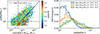 |
Fig. 1. Left: cosmoDC2 halo M200c masses (from the simulation) versus the redMaPPer cluster richnesses. The points are colored with the redMaPPer cluster redshift. The solid line is the best-fitted mean richness-mass relation in Eq. (16) at z = 0.4. The dashed lines represent the low mass and low richness cut used on the cosmoDC2-redMaPPer matched catalog for the fit of the fiducial scaling relation. Right: Histogram of richnesses in bins of mass, and best-fit probability distributions P(lnλ|M, z) from Eq. (15) (solid lines) for the different mass bins. |
3.4.1. The fiducial mass-richness relation
From the cosmoDC2-redMaPPer matched catalog, we can infer a “fiducial” scaling relation. We consider the fiducial set to be the set of clusters with λ > 10 (horizontal dashed line in Figure 1, left panel), as well as M > 4 × 10¹³ M⊙ (vertical dashed line) and with 0.2 < z < 1. The fiducial likelihood is given by
 (18)
(18)
where P(lnλk|Mk, zk) is the mass-richness relation given in Eq. (15) for the k-th cluster-halo match (we consider the pivot redshift z0 = 0.5 and pivot mass m0 = 1014.3 M⊙), and the subscript denotes truncated Gaussians with λk > λmin = 10. We use the emcee package Foreman-Mackey et al. 2013, with flat priors inspired by Murata et al. 2019, as listed in Table 1 (second column). The best-fitted fiducial relation is shown in the third column of Table 1. These values can serve as a reference against which we we compare the results obtained using cluster weak lensing and abundance.
Fiducial values of the parameters of the redMaPPer cluster mass-richness relation.
The low-mass richness cuts applied to the matched catalog are deliberately conservative. These cuts are chosen to ensure that the completeness of the redMaPPer cluster catalog (see Sect. 3.4.2) does not influence the inference of the fiducial cluster scaling relation. In Appendix A we examine the impact of alternative cuts, motivated by the modeling of the mass-richness relation used in this work. While this topic warrants further investigation, for this study, we adopt the fiducial values listed in Table 1.
We show, over-plotted in black in the left panel of Figure 1, the mean scaling relation for the best-fit parameters at z = 0.4. The right panel of Figure 1 presents the normalized histograms of redMaPPer richness in three different mass bins (within the redshift range z ∈ [0.2, 1]). Over-plotted on these histograms is the best-fit probability density function, P(λ|mcenter, zcenter), where zcenter and mcenter represent the center values of each redshift-mass bin. We observe that the predicted distribution matches the observed one quite well.
3.4.2. The redMaPPer selection function in DC2
To properly model cluster number counts, we must account for the selection function Φ of the redMaPPer algorithm (see, e.g., Euclid Collaboration 2019; Lesci et al. 2022). Defined in Eq. (3), the selection function reflects the fact that the cluster-finding algorithm may miss a fraction of true galaxy clusters (completeness) as well as detect “false” clusters that are not associated with underlying collapsed dark matter structures (purity).
From the matched catalog, we can disentangle the effects of purity and completeness within narrow mass-redshift-richness bins. The measured completeness  in the mass and redshift bins [mi, mi + 1] and [zj, zj + 1], and the measured purity
  in the richness and observed redshift bins [λk, λk + 1] and [zobs, l, zobs, l + 1], are given by
 (19)
(19)
where  is the total number of halos in the ij mass-redshift bin, and
  is the number of redMaPPer clusters in the kl richness-redshift bin. The quantity
  (respectively
  ) is the number of halos that have been matched to redMaPPer clusters in the ij mass-redshift bin (respectively in the kl richness-redshift bin). We model the observed completeness
  and purity
  , allowing them to be included in the count/lensing formalism as detailed in Sect. 2. The performance of the DC2 redMaPPer cluster catalog is analyzed in detail in Ricci et al. (in prep.). We note that the redMaPPer cluster catalog is complete at the 80% level for M200c > 1014 M⊙, with a small redshift dependence, and is pure at the > 90% level for λ > 12.
4. Methodology to constrain the mass-richness relation
As shown in Sect. 2, the modeling of cluster number counts and/or cluster lensing (with stacked excess surface density profiles or mean cluster masses) in bins of redshift and richness depends on the mass-richness relation. To constrain the parameters of the latter using this observables requires building the corresponding data vectors (Sect. 4.1) and defining the likelihood functions that link the data vectors, the covariances, and the models for each of these observables, as described in (Sect. 4.2). These likelihoods may then be used individually or in combination to constrain the parameters of the mass-richness relation. To implement the methodology described in this section, we rely on a variety of software tools that are briefly listed in Sect. 4.3.
4.1. Data vectors
We turn to the construction of the data vectors that will be used for the inference of the redMaPPer cluster mass-richness relation. For the stacking strategy we employ, we considered the redshift bin edges zi = 0.2, 0.3, 0.4, 0.5, 0.6, 0.7, 0.8, 1 and the richness bin edges λi = 20, 35, 70, 100, 200. We use λ > 20 and z > 0.2, inspired by other redMaPPer-based cluster analyses (see, e.g., McClintock et al. 2019; DES Collaboration 2020). The λ > 20 cut ensures a high-purity cluster sample Costanzi et al. 2019, close to 100% pure in our case, and restricting to z > 0.2 mimics the conservative cut used in DES cluster-based analyses DES Collaboration 2020, 2025. This cut was implemented to prevent the degradation of redMaPPer performance at low redshifts20, where the red-sequence galaxy population becomes harder to isolate due to the lack of u-band data in DES (which used g, r, i, and z bands). We note that robust detection of low-redshift clusters below z = 0.2 will be feasible with LSST, since u-band imaging will be available.
4.1.1. Cluster number counts
We show in Figure 2 the measured count of redMaPPer clusters as a function of richness for different redshift bins. As expected, there are fewer clusters at higher richness than at lower richness.
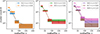 |
Fig. 2. Measured count of redMaPPer cluster as a function of richness, for different richness bins. For each richness-redshift bin, the width of the shaded area represent the width of the richness bin, and the height correspond to the Poisson noise |

4.1.2. Stacked excess surface density profiles
Considering an ensemble of Nl clusters (or “lenses”), where each cluster has Nls background source galaxies in the radial bin [R − ΔR/2, R + ΔR/2], the maximum likelihood estimator of the stacked ΔΣ(R) profile is given by Shirasaki & Takada 2018; Sheldon et al. 2004
 (20)
(20)
where the sum runs over all lens-source pairs and only for sources located within the physical projected radius interval, [R − ΔR/2, R + ΔR/2], from the lens l. Here, ϵ+l, s is the tangential ellipticity of the source galaxy, s, relative to the position of lens l, as given by Eq. (6). The quantity  is the effective critical surface mass density of the lens-source system, averaged over the photometric redshift probability density function p(zs) of the galaxy with index s, such that
 (21)
(21)
The weights wls maximize the S/N for this estimator Sheldon et al. 2004 and can be written as the product  , such that
 (22)
(22)
 (23)
(23)
The quantity σrms(ϵs+) = σSN is the intrinsic galaxy shape noise of the ellipticity’s tangential component, arising from the fact that unlensed galaxies have an intrinsic distribution of ellipticities and position angles (see, e.g., Pranjal et al. 2023; Chang et al. 2013). In cosmoDC2, the intrinsic shape noise for each galaxy’s ellipticity component is σSN = 0.2521, which is comparable to what has been found in the literature Chang et al. 2013. In contrast, σmeas(ϵs+) represents the uncertainty originating from galaxy ellipticity estimation on images (see, e.g., Hirata & Seljak 2003; Mandelbaum et al. 2005; Sheldon & Huff 2017). In the ideal case of cosmoDC2, where galaxy redshifts and shapes are perfectly measured, these weights reduce to  and
and  , where only the intrinsic variation of galaxy shapes remains.
The evaluation of the  data vector relies on a selection of background sources. The source selection is initially based on an r-band magnitude cut of r < 28 and an i-band magnitude cut of i < 24.25, aiming to reach a number density of galaxies ngal ≈ 25 arcmin−2, comparable to the number density expected in the context of LSST after 10 years of data Chang et al. 2013. For each cluster in the redMaPPer catalog, we then extract the galaxy source catalog in a circular aperture of R = 10 Mpc, applying the source selection zs > zl + 0.222, where zs is the true cosmoDC2 galaxy redshift and zl is the redMaPPer cluster redshift23.
We constructed each source galaxy lensed ellipticity ϵobs from Eq. (5) using (i) its intrinsic shape ϵint and (ii) the shear and convergence values at the galaxy’s location that are provided in the cosmoDC2 catalog. For each stack of Nl clusters, we consider 10 log-spaced radial bins from 0.5 Mpc to 10 Mpc and estimate the stacked lensing profile using Eq. (20).
The corresponding excess surface density profiles are displayed in Figure 3 as a function of the distance to the cluster center, for different richness bins and different redshift bins. At fixed richness, we do not observe a particular trend with redshift at scales larger than 1 Mpc, as denoted by the vertical dashed lines.
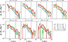 |
Fig. 3. Stacked excess surface density profile as a function of the distance to the cluster center, for different richness bins (colors) and different redshift bins (from top left to bottom right). The error bars are the diagonal elements of the bootstrap covariance matrices. The dashed black vertical line (resp. black filled vertical line) represents the R > 1 Mpc cut (resp. R < 3.5 Mpc cut). |
However, for R < 1 Mpc, we observe that the stacked lensing profiles are progressively attenuated in the innermost regions with redshift. This attenuation has already been observed in DC2 galaxy-galaxy lensing Korytov et al. 2019 and cluster-galaxy lensing Kovacs et al. 2022 and is associated with the limited resolution of ray tracing used to compute the lensing shear and convergence at each galaxy position in the simulation. As a consequence, we chose to use only the R > 1 Mpc region for each stack in the analysis. This choice is valid across the full richness and redshift range. However, it also means that we cannot use the innermost regions with the largest S/N values. This intrinsic limitation will constrain the cluster-related forecasts of what could be achieved with the LSST data. We show in Figure 4 the S/N of some excess surface density profiles for a low (left panel) and a high (right panel) redshift bins. In the considered redshift range, the S/N oscillates between 2 and 13 for the low-redshift bin, and between 0.5 and 8 for the high redshift bin. The profiles in the last richness bin have the lowest S/N, due to the low statistics in these bins (with ∼10 times fewer clusters than in the first richness bin). Let us note that the stacking strategy allows us to significantly increase the S/N, as the S/N of individual cluster excess surface density profiles (not shown here) ranges from 0.1 to 324.
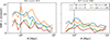 |
Fig. 4. S/Ns of the stacked excess surface density profiles, for two different richness bins (left and right panel) and different richness bins (colors). |
4.1.3. Mean cluster masses
As mentioned earlier in this paper, instead of directly using the stacked profiles for weak-lensing information to constrain the mass-richness relation, we can use the corresponding mean cluster lensing masses as an alternative data vector. To do so, for each ij-th redshift-richness bin, we first need to infer the mean cluster mass  and its corresponding error
  from the corresponding stacked lensing profile
  .
.
This is done by fitting, for each bin, a dark matter density profile25 to the corresponding stacked lensing profile obtained in Sect. 4.1.2 using the Minuit26 minimizer James & Roos 1975, which is much faster than an MCMC. We ensured that the recovered mass and error from Minuit coincide at the < 0.1σ level with the mean mass and errors inferred from an MCMC procedure.
We used a NFW profile Navarro et al. 1997 with the concentration-mass relation of Duffy et al. 200827. We show in the left panel of Figure 5 the inferred mean cluster masses as a function of richness for the different redshift bins after fitting the stacked profiles within the radial range28R ∈ [1, 3.5] Mpc. The error bars on the y-axis correspond to the statistical error obtained from our fitting procedure of the cluster mass, while the x-axis error represents the dispersion of richness values in each bin.
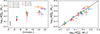 |
Fig. 5. Left: Mean cluster lensing mass as a function of mean richness within the stack, the different colors correspond to the different redshift bins. Right: Mean cluster lensing masses as a function of the DC2 matched masses from the cosmoDC2 dark matter halo catalog. The different colors correspond to the different redshift bins. The dashed line corresponds to y = x. |
For validation, we compared the recovered mean lensing mass to the true mean mass in each redshift-richness bin in the right panel of Figure 5, where the true masses are obtained by (i) matching the redMaPPer cluster catalog to dark matter halos (ii) computing the corresponding cosmoDC2 mass in each redshift-richness bin. We see a clear correlation between weak lensing mean masses and cosmoDC2 masses (we added the one-to-one line x = y to allow for a visual comparison).
4.2. Likelihoods and priors
After building the data vectors, we turned our attention to inferring the parameters of the mass-richness relation defined in Sect. 2.3, namely θ = (lnλ0, μz, μm, σlnλ0, σz, σm). We adopted the pivot redshift z0 = 0.5 and pivot mass m0 = 1014.3 M⊙ in the mass-richness relation in Eq. (16).
4.2.1. Cluster count likelihood
We considered the cluster count likelihood Hu & Kravtsov 2003 given by
![Mathematical equation: $$ \begin{aligned} \mathcal{L} _{\rm N} \propto |\Sigma _{\rm N}|^{-1/2}\exp -\frac{1}{2}\sum _{ijkl}(N-\widehat{N})_{ij}\,[\Sigma _{\rm N}]^{-1}[ij,kl]\,(N-\widehat{N})_{kl} . \end{aligned} $$](/articles/aa/full_html/2025/08/aa54107-25/aa54107-25-eq41.gif) (24)
(24)
In the above equation, the index ij (resp. kl) refers to the i-th redshift bin and the j-th richness bin (respectively the k-th redshift bin and the l-th richness bin).  (resp. Nij) denotes the measured (resp. predicted) cluster count in the ij-th redshift-richness bin. For the count prediction, we adopted mmin = 1012 M⊙ and mmax = 1015.5 M⊙ as the minimum and maximum halo masses for the integration of the halo mass function of Despali et al. 2015 in Eq. (1). The best-fit selection function, Φ, as described in Sect. 3.3, is used in Eq. (1). The quantity ΣN is the cluster count covariance matrix, which accounts for two contributions: the Poisson shot noise and the super-sample covariance (SSC). First, the Poisson noise affects the counting of clusters in uncorrelated bins Poisson 1837. Second, the SSC denotes the contribution from the intrinsic fluctuations of the matter overdensity field, within and beyond the survey volume Hu & Kravtsov 2003. As a result, SSC introduces a covariance between the counts in different bins and increases their variance. SSC is particularly important in cluster abundance-based likelihoods, as it impacts the precision of the recovered cosmological parameters by approximately 20% for surveys such as the Vera C. Rubin Observatory’s LSST or the Euclid mission Fumagalli et al. 2021; Payerne et al. 2023, 2024, which are each expected to detect hundreds of thousands of clusters. The shot-noise and SSC contributions to the total covariance can, in principle, be estimated through resampling techniques directly on the data, such as jackknife resampling Escoffier et al. 2016. However, due to the relatively small number of clusters detected in the DC2 galaxy catalog, jackknife estimates of the cluster count covariance matrix suffer from high noise. We therefore opt to use a theoretical prediction for the covariance instead, given by
![Mathematical equation: $$ \begin{aligned} \Sigma _{\mathrm{N} }[ij,kl] = N_{ij}\, \delta ^K_{ik}\,\delta ^K_{jl}+ N_{ij}\,N_{kl}\,\langle b\rangle _{ij}\,\langle b\rangle _{kl}\, S_{ik}. \end{aligned} $$](/articles/aa/full_html/2025/08/aa54107-25/aa54107-25-eq43.gif) (25)
(25)
The first term in Eq. (25) represents the Poisson shot noise, with δikK denoting the Kronecker delta function. The second term corresponds to SSC, where Sik = ⟨δm, iδm, k⟩ is the covariance of the smoothed matter overdensities δm in the i-th and k-th redshift bins, respectively Lacasa et al. 2018. The coupling between the matter overdensity field and the halo number density field is encoded by the halo bias b(m, z) Tinker et al. 2010, which depends on mass and redshift and is averaged over the ij-th (resp. kl-th) redshift-richness bin to yield ⟨b⟩ij (resp. ⟨b⟩kl). Finally, Nij is the model prediction for the number of clusters in the ij-th redshift-richness bin, as defined in Eq. (4). This likelihood model, which incorporates both Poisson noise and SSC, has been adopted in previous cluster analyses, for instance, by DES Collaboration 2020; Costanzi et al. 2019; Sunayama et al. 2024.
4.2.2. Stacked lensing profile likelihood
We can constrain the mass-richness relation by using the stacked excess surface density profiles directly Murata et al. 2019; Park et al. 2023; Sunayama et al. 2024. The likelihood for stacked excess surface density profiles, denoted ℒWLp, is given by
![Mathematical equation: $$ \begin{aligned} \mathcal{L} _{\Delta \Sigma }\propto \exp -\frac{1}{2}\sum _{ij}(\Delta \Sigma -\widehat{\Delta \Sigma })_{ij}\,\Sigma ^{-1}_{\Delta \Sigma }[ij]\, (\Delta \Sigma -\widehat{\Delta \Sigma })_{ij}. \end{aligned} $$](/articles/aa/full_html/2025/08/aa54107-25/aa54107-25-eq44.gif) (26)
(26)
Here,  corresponds to the stacked excess surface density profile estimated in Eq. (20) for the ij-th redshift-richness bin, ΔΣij is the corresponding theoretical prediction from Eq. (13), and ΣΔΣ[ij] denotes the associated covariance matrix. This covariance originates from a variety of phenomena, as discussed in Hoekstra 2003; Wu et al. 2019; Gruen et al. 2015; McClintock et al. 2019. A primary contribution is the intrinsic scatter in the shapes of background galaxies, combined with the limited number of clusters and source galaxies within each bin. This term, often referred to as shape noise, dominates the small-scale regime but can be reduced by increasing the sample size. Another significant contribution comes from uncorrelated large-scale structures along the line of sight, which introduce stochastic fluctuations in the lensing signal unrelated to the lensing cluster. In addition, correlated structures around the cluster – such as nearby halos and filaments – affect the lensing profile through variations in the two-halo term, thereby contributing an additive component to the covariance. At smaller scales, intrinsic variations in the properties of halos within each stack, including the scatter in concentration at fixed mass, halo ellipticity, and orientation, also contribute to the overall uncertainty. Finally, the spread in true halo masses among richness-selected clusters within a given bin introduces further variance in the measured lensing profiles.
As for cluster counts, the covariance of the cluster lensing profiles can be predicted analytically (see, e.g., Wu et al. 2019)29 or using semi-analytical approaches (see, e.g., McClintock et al. 2019). These methods require modeling a wide range of data properties, including the redshift distributions of the source and lens samples, the dispersion of intrinsic galaxy shapes, the dark matter halo density profile, and the level of scatter in concentration, miscentering, and morphology of clusters in the redMaPPer catalog. In our case, we choose a simpler, data-driven approach that estimates all these contributions simultaneously without relying on model assumptions, while also keeping computational costs relatively low. Specifically, we use bootstrap resampling (see, e.g., Simet et al. 2017; Parroni et al. 2017) with Nboot = 400 resampled cluster ensembles. We retain only the diagonal terms of the covariance matrices, as the off-diagonal elements are too noisy due to the limited cluster count statistics in each richness-redshift bin within the DC2 footprint. Wu et al. 2019 point out that neglecting off-diagonal terms at large scales (R ≳ 5–6 Mpc) can lead to an underestimation of parameter uncertainties inferred from weak-lensing profiles – such as cluster mass and concentration – especially when shape noise (i.e., uncorrelated sources of noise) is subdominant. However, since our analysis focuses exclusively on the R < 3.5 Mpc regime, this impact is expected to be minimal. Therefore, we assume diagonal covariance matrices throughout, as the off-diagonal terms remain extremely noisy Phriksee et al. 2020.
4.2.3. Mean cluster mass likelihood
The cluster mass-richness relation can also be inferred using the information from mean mass estimates McClintock et al. 2019; DES Collaboration 2020; Lesci et al. 2022. Then, the mean mass likelihood is given by
 (27)
(27)
where log10Mij is the mass prediction that is given in Eq. (14) in the ij-th redshift-richness bin, and  is the measured mean mass.
It is important to highlight the differences between the one-step approach (described in Sect. 4.2.2) and the two-step approach (discussed in this section). The one-step approach offers greater flexibility. Specifically, it allows for more comprehensive modeling of various systematic effects that influence the lensing signal, including cluster miscentering, projection effects from both correlated and uncorrelated large-scale structures, contamination by cluster member galaxies, and deviations from spherical symmetry in the cluster mass distribution compared to the two-step approach. However, the one-step approach presents a significant computational challenge, as it necessitates marginalizing over numerous theoretical and observational effects Aguena et al. 2023, compared to the two-step approach.
4.2.4. Total likelihood and priors
To infer the parameters of the mass-richness relation, the total likelihood ℒtot is given by considering either counts, cluster lensing profiles, or cluster lensing masses, or the combination between counts and cluster lensing, namely,
 (28)
(28)
It is important to note that the way the lensing and count likelihoods are combined assumes no covariance between the two. As shown by Costanzi et al. 2019, the cross-correlation between the abundance and weak lensing inferred quantities is consistent with zero.
We drew samples from the parameter posterior distribution given by
 (29)
(29)
where θ = (lnλ0, μz, μm, σlnλ0, σz, σm), ℒtot(data|θ) is the total likelihood in Eq. (28) (ℒtot(data) is the likelihood evidence) where “data’ refers to either the stacked lensing profiles, the inferred mean lensing masses, the cluster counts, or combinations of abundance and lensing information.
To compute the prior π(θ), we consider the choices made for the fiducial mass-richness relation and summarized in the second column of Table 1. All fits are performed at a fixed cosmology, chosen to be the fiducial cosmology of the DC2 simulation, which is close to the seven-year Wilkinson Microwave Anisotropy Probe (WMAP) best-fit Λcold dark matter values Komatsu et al. 2011 given by h = H0/100 = 0.71 (the reduced Hubble constant H0), Ωcdmh2 = 0.1109 (Ωcdm is the current fractional energy density associated with cold dark matter), Ωbh2 = 0.02258 (Ωb is the current fractional energy density associated with baryons), ns = 0.963 (spectral index of the primordial power spectrum), σ8 = 0.8 (dispersion of matter density fluctuations smoothed over 8 h−1 Mpc), and w = −1 (dark energy equation of state).
4.3. Software
This work allows us to demonstrate the use of some of the software tools developed in DESC (in combination with others) for concrete cluster analysis. For this work, we use several DESC software tools that are currently in development as part of the DESC pipeline for analyzing the upcoming LSST data. To extract the cluster, halo, and background galaxy catalogs from the DC2 dataset, we used the DESC package GCRCatalogs30, along with Qserv31, an open-source SQL database system (Massively Parallel Processing) originally designed to host LSST data. For the estimation of the stacked lensing profiles, we used the DESC Cluster Lensing Mass Modeling (CLMM; Aguena et al. 2021b) package32, which provides various tools for estimating cluster lensing profiles as well as for halo modeling. The Core Cosmology Library33 (CCL; Chisari et al. 2019) was used to predict the halo mass function, halo bias, and concentration-mass relations. A combination of these codes was produced within the LSSTDESC/CLCosmo_Sim repository34. To compute the binned Sij terms for the cluster count covariance in Eq. (25), we use the PySSC35 package Lacasa et al. 2018; Gouyou Beauchamps et al. 2022. Cluster scaling relation parameters were inferred using the Markov chain Monte Carlo (MCMC) implementation in the emcee package Foreman-Mackey et al. 2013, with visualization performed via getdist Lewis 2019. Finally, we also use the Minuit36 minimizer James & Roos 1975 to fit the mean cluster mass per redshift-richness bin in the two-step procedure.
5. Results
All the ingredients are now in place to perform the analysis of the scaling relation of redMaPPer clusters. In Sect. 5.1, we begin by presenting the setup that serves as our baseline analysis. Subsequent sections present variations of this baseline, changing one ingredient at a time. Sect. 5.2 explores how the modeling choices for the halo density and mass-concentration relation impact the results, while Sect. 5.3 focuses on observational systematic effects, specifically the impact of source photometric redshifts and the shear-richness covariance. Table 2 summarizes the tables and figures associated with the different study cases.
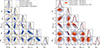 |
Fig. 6. Left: Posterior distribution of the scaling relation parameters using abundance alone (blue), lensing profiles alone (dashed red), or masses alone (solid green lines). The joint abundance and lensing profiles posterior is displayed in black. Right: Posterior distribution of scaling relation parameters when combining abundance and lensing profiles (solid blue lines) and combining abundance and cluster masses (orange-filled contours). The dashed contours are obtained by removing the last redshift bin for both abundance and lensing. |
5.1. Defining the count and weak lensing baseline analyses: N + MWL versus N + ΔΣ
We model the per-cluster excess surface density, ΔΣ(R|m, z), using a three-dimensional dark matter density profile given by
 (30)
(30)
For n = 2, the Eq. (30) corresponds to the NFW profile Navarro et al. 1997. Then, rs = r200c/c200c is the scale radius, and ρs is the scale density37. We use the concentration mass-relation of Duffy et al. 2008 (see 5.2.1 hereafter).
We restricted the fitting to 1 < R < 3.5 Mpc. The typical value of Rmax = 3.5 Mpc is inspired by Lee et al. 2018, Giocoli et al. 2021, Cromer et al. 2022, Murray et al. 2022, and Bocquet et al. 2024 and is typically the distance beyond which the two-halo term increasingly dominates the cluster lensing signal and cannot be neglected (this choice is discussed further in Appendix B and later in the text).
We show in the left panel of Figure 6 the 68% and 95% credible intervals on the cluster scaling relation when using (separately) the cluster abundance likelihood, stacked lensing profiles, or mean cluster masses. The vertical and horizontal lines represent the fiducial values of the redMaPPer cluster scaling relation inferred in Sect. 3.4.1. We observe that the abundance provides tighter constraints on the mean parameters, but has different degeneracies compared to lensing (either stacked profiles or mean masses). The contours exhibit characteristic degeneracies and significant overlap, which suggests they can be combined. Additionally, we note that the posteriors are fairly compatible with the fiducial constraints at the 1–2σ level.
The different degeneracy directions between the abundance and lensing contours provide tight final constraints on the scaling parameters when combined38. By combining abundance with lensing, we obtain the posteriors shown in the right panel of Figure 6, either with stacked profiles or mean masses39. We observe that using either mean masses or stacked profiles provides roughly the same constraints with comparable precision. The errors on the mean scaling parameters (lnλ0, μz, and μm) are reduced by a factor of ∼7, while the errors on the scatter terms (σlnλ0, σz, and σm) are reduced by a factor of ∼3 − 4. The one-dimensional posteriors obtained from our joint lensing and abundance likelihood fairly recover the fiducial values at the < 2σ level; however, we observe a > 2σ tension with the projected posterior on μz − σz.
We checked whether the stacked lensing profiles in the last redshift bin are still impacted by the ray-tracing shear resolution beyond R = 1 Mpc, despite our conservative radial cut, since the attenuation increases with redshift and is therefore maximal in the last bin. To assess this, we removed the last redshift bin from the estimation of the posterior (from both abundance and lensing profiles). This yields results compatible with our baseline analysis, albeit with wider error bars (the last redshift bin contains 30% of the full cluster catalog). This provides a sanity check for our lensing and count pipeline, which offers a reasonable comparison to the “fiducial” constraints of the redMaPPer mass-richness relation. Residual systematics inherent to our analysis – such as the calibration of the halo mass function and uncertainties in the selection function – may still induce some bias in the recovered parameters.
We also examine in Appendix B the impact of alternative Rmax cuts on the scaling relation parameters. We find that using the fully available radial range (up to Rmax = 10 Mpc) without modeling the two-halo term yields results comparable to those obtained with the baseline Rmax = 3.5 Mpc cut, showing only small biases (< 1σ) and similar error bars. This is attributed to the noisy lensing measurements at larger scales, which diminish the impact of the two-halo term and do not provide additional constraining power. We adopt the Rmax = 3.5 Mpc cut throughout this work. However, the two-halo term cannot be neglected for larger datasets, which will provide a larger S/N in the two-halo regime. In the following, we consistently use the combination of lensing (either mean masses or stacked profiles) and cluster counts to probe the underlying cluster scaling relation, leveraging their complementarity in parameter space.
5.2. Impact of modeling choices (in the N + MWL framework)
The inference of the cluster scaling relation is impacted by several systematic effects, stemming from the many degrees of freedom in the modeling of cluster observables. The choice of a particular mass distribution model can significantly affect the inferred cluster lensing mass and, consequently, have a non-negligible impact on the mass-richness relation. We restricted our analysis to the one-halo regime, namely at scales below R = 3.5 Mpc, which is more sensitive to the internal halo properties (such as cluster mass and concentration) than the two-halo regime, which is primarily influenced by cosmological quantities through the power spectrum and halo bias Oguri & Takada 2011.
5.2.1. Concentration–mass relation
As mentioned in Sect. 2, the cluster density profile depends on the concentration parameter c200c. Cosmological simulations indicate that cluster concentration and mass are statistically correlated. This correlation is typically quantified by a fitting formula known as the concentration-mass relation, labeled c(M). The concentration c of an individual cluster with mass M is then scattered around c(M), with a dispersion denoted σc|M. Several c(M) relations exist in the literature (see, e.g., Diemer & Kravtsov 2014; Duffy et al. 2008; Prada et al. 2012; Bhattacharya et al. 2013; Diemer & Joyce 2019). For example, our baseline choice in Sect. 5.1 adopts the c(M) relation of Duffy et al. 2008, calibrated using N-body simulations based on the five-year WMAP cosmology Komatsu et al. 2009, which differs by at most 5% from the seven-year WMAP cosmology Komatsu et al. 2011 used in cosmoDC2. The alternative relations examined in this section Prada et al. 2012; Bhattacharya et al. 2013; Diemer & Kravtsov 2014 have been shown to accurately describe the relationship between halo mass and concentration across a variety of Λ cold dark matter cosmologies. These relations, despite some intrinsic scatter, capture the general trend observed in simulations. Employing such a relation can reduce the number of free parameters in cluster-based analyses and thus improves constraints on other relevant parameters.
To test the impact of the c(M) relation on the scaling relation parameters, we (i) fit the mean cluster masses using various c(M) relations from the literature (where M denotes the mean mass, considered as a free parameter), (ii) use these mean mass estimates in Eq. (27), and (iii) combine them with the cluster count likelihood from Eq. (24) to infer the scaling relation parameters. Alternatively, the concentration can be treated as a free parameter in each redshift-richness bin. In this case, we jointly fit the concentrations and mean masses in each bin and use the resulting mass estimates in the mass likelihood.
In the left panel of Figure 7 the concentration-free case shows reasonable agreement with the fiducial constraints. The posteriors obtained using different concentration-mass relations are fully consistent with the free-concentration case. When adopting a fixed c(M) relation, the inferred posteriors exhibit the same level of parameter correlation, with slightly reduced error bars due to the smaller number of free parameters in the fitting procedure. We note that the choice of concentration model is expected to have a larger impact in the inner regions (R < 1 Mpc), which are not probed here due to the limitations imposed by ray-tracing resolution.
5.2.2. Modeling of the matter density profile
Besides the NFW parameterization, Einasto 1965 suggested an empirical profile that has been shown to provide a slightly better fit to N-body simulations of galaxy clusters compared to the NFW profile – particularly at small scales and over a broad range of halo masses and redshifts Klypin et al. 2016; Sereno et al. 2016; Wang et al. 2020. The corresponding three-dimensional density profile is given by
![Mathematical equation: $$ \begin{aligned} \rho ^\mathrm{ein}(r) = \rho _{-2}\exp \left(-\frac{2}{\alpha }\left[\left(\frac{r}{r_{-2}}\right)^\alpha - 1\right]\right), \end{aligned} $$](/articles/aa/full_html/2025/08/aa54107-25/aa54107-25-eq51.gif) (32)
(32)
where r−2 = r200c/c200c and the ρ−2 is given in the footnote40. In the above equation, α is the shape parameter. We adopt a typical constant value of α = 0.25, though it is worth noting that more sophisticated models incorporate mass, redshift, and cosmology dependence in α, as observed in simulations Gao et al. 2008. In such models, α typically ranges from 0.15 to 0.3 as a function of mass. Less commonly, the Hernquist density model (corresponding to n = 1 in Eq. (30)) has been used, for example, in Buote & Lewis 2004; Sanderson & Ponman 2009 to model the mass density of X-ray-detected galaxy clusters, though it has not been extensively used in the lensing literature.
Concentration-mass relations for the Einasto and Hernquist models have not been extensively studied in the literature. Therefore, we consider the fit without assuming a specific c(M) relation, prioritizing the count/mass cluster likelihood instead. In the right panel of Figure 7, we show the posterior distribution of the scaling relation parameters when considering the count/mass likelihood, using the NFW, Einasto, and Hernquist profiles. The results are in good agreement with each other, likely due to the radial range used in the fit, where the profiles are similar and only start to diverge at smaller scales. By fitting the mean cluster mass from 1 Mpc to 3.5 Mpc, where the one-halo regime is dominant, and using either the NFW, Einasto, or Hernquist profile, we found that the inferred scaling relation remains fairly stable.
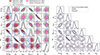 |
Fig. 7. Left: Posterior distribution of the scaling relation parameters using count/mass likelihood. The concentration-free case is shown with the dashed lines, the other contours are obtained using various concentration-mass relations from the literature. Right: Posterior distribution of the scaling relation parameters using count/mass likelihood, without using a concentration-mass relation, and using different modeling of the cluster density profile, namely NFW (red filled contours), Einasto (solid lines), and Hernquist (dashed lines). |
5.3. Observational systematic effects (in the N + ΔΣ framework)
We addressed several potential sources of bias arising from uncertainties in the modeling of the cluster lensing observable. Another major source of bias in cluster lensing analyses comes from the data itself, including the calibration of galaxy shapes Hernández-Martín et al. 2020, the redshift distribution of the background galaxy sample Wright et al. 2020, contamination of the source galaxy sample by foreground galaxies Varga et al. 2019, and miscentering in the cluster catalog Sommer et al. 2022.
Using the cosmoDC2 catalog, we rely on the true shapes of galaxies (i.e., accounting only for the intrinsic shape and local shear), and thus cannot investigate the effects of shape measurement errors with this dataset. In the following, we focus instead on the impact of the calibration of the background galaxy photometric redshift distribution on the cluster scaling relation (Sect. 5.3.1), as well as on the impact of shear-richness covariance (Sect. 5.3.2). With this simulated dataset and the analysis choices we made, the effects of miscentering and contamination of the source sample by cluster members, which generally need to be accounted for, are not significant; they are discussed in Appendices C.1 and C.2, respectively.
5.3.1. Source galaxy photometric redshifts
In Sects. 5.1 and 5.2, we use the true galaxy redshifts to compute the geometrical lensing weights  . In contrast, with imaging data, each source galaxy behind clusters is assigned a photometric redshift distribution, derived from galaxy magnitudes measured in several optical bands. The uncertainty in the measured redshift can be incorporated into the lens-source geometrical weights through Eq. (21).
In this section, we test the impact of using the BPZ Benítez 2011 and FlexZBoost Izbicki & Lee 2017 output photometric redshifts on the inference of the cluster scaling relation. To do this, we modify the source selection, which is now based on photometric-related quantities. Figure 8 shows the mean photometric redshift and its dispersion as a function of the true cosmoDC2 redshift (no quality cut is applied to the photometric-derived quantities). As FlexZBoost provides robust estimates up to z = 3, BPZ yields more dispersed and biased results, making the use of BPZ redshifts without quality cuts problematic above z ∼ 2, and potentially biasing the constraint of the mass-richness relation. The increased dispersion and bias of BPZ estimates at higher redshifts is not unexpected, as the model photometry in the simulation included a nonphysical dust feature in some SEDs at high redshift that was not present in the SED templates used to compute theoretical fluxes by BPZ, leading to a bias and increased dispersion.
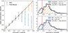 |
Fig. 8. Left: Mean photometric redshift against true cosmoDC2 redshift for BPZ and FlexZBoost methods. Right: Distribution of true cosmoDC2 redshifts after our magnitude cuts (black). Upper panel: The blue distribution represents the same distribution after a cut on the probability P(zs > zl) using FlexZBoost photometric redshift, for a cluster at z = 0.38. The orange distribution is obtained after combining the P(zs > zl) cut and the mean redshift cut. Lower panel: Same as upper panel but for BPZ redshifts. On both panels, the vertical red line indicates the position of the cluster redshift. |
As discussed in Sect. 3, none of these estimations are realistic due to (i) the deep selection of the training sample up to i < 25 for FlexZBoost, which makes the results optimistic, and (ii) the “discreteness” in the color-redshift space of the modeled galaxies Korytov et al. 2019, which negatively impacts the performance of BPZ. Updated redshifts are currently being produced by DESC. These updated redshifts were not available at the time of this work, so we proceeded with the first version of the photometric redshift catalogs. The actual LSST data will likely fall between the pessimistic BPZ and optimistic FlexZBoost runs we use. By considering both approaches, we can bracket the impact of photometric redshifts on the results.
For the source sample selection, we apply two cuts simultaneously: (i) based on the mean photometric redshift, namely, ⟨zs⟩> zl + 0.2, and (ii) based on the probability density function, with P(zs > zl) > 0.8, where
 (34)
(34)
is the probability for a galaxy to be located behind the cluster. In the above equation, p(zs) is the galaxy photometric redshift distribution (obtained either from BPZ or FlexZBoost). Moreover, we do not apply any quality cut on the photometric redshifts, allowing us to test the robustness of the cluster scaling relation with respect to photometric redshifts in the “worst-case” scenario; namely, with no mitigation of the impact of outliers on the final results. We show in Figure 8 (right, upper panel) the distribution of true galaxy redshifts in cosmoDC2 after our magnitude cuts. We also show the background source sample after applying the P(zs > zl) cut alone and after combining the P(zs > zl) and mean redshift cuts on FlexZBoost redshifts, for a redMaPPer cluster at redshift z = 0.38. We see that our photometric source selection efficiently removes foreground and member galaxies. The same distributions are shown in Figure 8 (right, lower panel) for BPZ redshifts.
We show in Figure 9 the constraints on the scaling relation when considering photometric redshifts from either BPZ (left panel) or FlexZBoost (right panel). Using BPZ introduces a small negative bias of ∼1σ in the normalization of the scaling relation, as well as in the mass dependence, compared to the true redshift case.
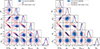 |
Fig. 9. Impact of photometric redshifts of source galaxies on scaling relation parameter estimation. Left: The filled contours show the constraints when using true redshifts of source galaxies. Dashed contours are obtained when considering the BPZ photometric redshifts. Empty contours are obtained using BPZ photometric redshifts, after marginalizing over the (1 + b) correcting factor, considered as a free parameter, used to correct from photometric redshift calibration issues. Right: same as left panel, but for FlexZBoost. |
We incorporate a simple model to account for a possible bias in photometric redshift calibration at the level of the stacked lensing profile model, as proposed by Simet et al. 2017. We correct the modeling of the stacked excess surface density profile in Eq. (13) in each redshift-richness bin by a unique multiplicative factor (1 + b), common to all redshift-richness bins. This factor (1 + b) is fitted jointly with the scaling relation parameters, using a flat prior of [ − 0.5, 0.5] for b. The results are shown in Figure 9. For BPZ, we see that adding a free parameter to the fit increases the size of the posteriors as expected and helps decrease the tension between the photometric redshift case and the true redshift case. We recover a negative bias b = −0.02 ± 0.03, which is compatible with 0 at the 1σ level. For FlexZBoost (right panel), we first observe that without correction, the constraints are fully compatible with the true redshift case. Adding (1 + b), we recover b = 0.02 ± 0.03, and although the error bars increase, the posteriors do not shift significantly.
5.3.2. Impact of shear-richness covariance
In this section, we discuss a systematic bias arising from selection biases in cluster finder algorithms. For optically selected clusters, one relatively unexplored category of cluster systematics is the covariance between the two cluster observables, first, the shear estimated from background galaxies and second the richness, as an outcome of cluster finders. This covariance was left unconstrained in previous cluster cosmology analyses McClintock et al. 2019; DES Collaboration 2020. This property covariance can induce additive biases that cannot be mitigated with increased sample size and reduced shape noise Nord et al. 2008; Evrard et al. 2014; Farahi et al. 2018; Wu et al. 2019. To achieve percent-level mass calibration of clusters, this new category of systematics must be accurately and precisely quantified Rozo et al. 2014; Zhou et al. 2024. In this work, we follow the prescription of Zhang et al. 2024 in modeling and quantifying the systematic uncertainty induced by the property covariance of optically selected clusters on the cluster scaling relation.
We make a note of the difference between intrinsic and extrinsic covariance. In Zhang et al. 2024 the authors measured the intrinsic covariance of cluster weak lensing observables by encircling galaxies within a three-dimensional physical radius around the halo to measure the “true” richness and second, measured the integrated dark matter density around the halo. This intrinsic contribution to the covariance originates from the galaxy assembly bias, the degree of which can be quantified by secondary halo properties (e.g., concentration, mass accretion rate, kinetic-to-potential energy ratio) that relate to the formation history of the cluster-sized halo. On the other side, the extrinsic covariance arises from systematic biases introduced by the cluster-finding algorithm, such as projection effects (see, e.g., Myles et al. 2021, 2025). In this work, we measure the total covariance (intrinsic + extrinsic) using the redMaPPer cluster finder to determine the observed richness and the galaxy shear as a proxy for the surface density. This realistic mock catalog introduces observational systematics such as photometric redshift uncertainty Graham et al. 2017 and shape noise Wu et al. 2019 for the galaxy shear signal and projection and percolation effects Costanzi et al. 2018, triaxiality bias Zhang et al. 2023 and a set of other observational and modeling systematics McClintock et al. 2019 related to a realistic cluster finder as redMaPPer.
Our goal is to model and correct for the systematic uncertainty in the estimated stacked lensing profiles in Eq. (20). From Evrard et al. 2014; Aihara et al. 2018; Wu et al. 2019; Zhang et al. 2024, the corrected stacked excess surface density profile is given by
![Mathematical equation: $$ \begin{aligned} \Delta \Sigma _{ij}^\mathrm{corr}&= \Delta \Sigma _{ij} + \ln (10)\frac{[\beta _1]_{ij}}{\mu _m} \times \langle \mathrm{Cov} (\Delta \Sigma , \ln \lambda |m,z)\rangle _{ij}, \end{aligned} $$](/articles/aa/full_html/2025/08/aa54107-25/aa54107-25-eq54.gif) (35)
(35)
where ΔΣij is given in Eq. (13), and [β1]ij is the average logarithmic slope of the Despali et al. 2015 halo mass function in the ij-th redshift-richness bin. For the latter, we compute [β1]ij once before running MCMC, using the fiducial cluster scaling relation, and we consider the denominator μm to be free. ⟨Cov(γ, lnλ|m, z)⟩ij is the averaged shear-richness covariance (see calculation details in Appendix D and also in Zhou et al. 2024), associated with potential selection bias in the cluster finder algorithms. The factor ln(10) is used to match the definition in Evrard et al. 2014. In the latter, we present the estimation of ⟨Cov(ΔΣ, lnλ|m, z)⟩ij, to be used in the estimation of the cluster scaling relation parameters.
While Zhang et al. 2024 observed a radially dependent covariance at small scales R < R200c due to cluster formation physics, because of the attenuation of the cluster lensing signal at small scales due to the ray tracing resolution, we focus, instead, on the R > 1 Mpc scales. From mock-cluster studies analyzing selection effects such as Sunayama et al. 2020; Wu et al. 2022; Zhou et al. 2024, the total bias (intrinsic+extrinsic) is close to null at small scales and increases at larger scales for R > R200c. For this reason, the covariance after applying the scale cut due to lensing attenuation may be sufficient for describing to impact of the total covariance.
We apply a kernel local linear regression Farahi et al. 2022 to find the best fit local mean with mass as the independent variable and ΔΣ(R) and lnλ as the dependent variables. Specifically, the residuals of ΔΣ and lnλ are taken around their local mean quantities ⟨ΔΣ ∣ m, z, R⟩ and ⟨lnλ ∣ m, z⟩ such as
 (36)
(36)
 (37)
(37)
and the covariance is measured around the local residuals, namely,
 (38)
(38)
It is important to note that as we remove the residual dependence of the mean mass on the covariance, the size of the covariance itself can still nonetheless be a function of (m, z), namely, the scatter and correlation are modeled as σlnλ|M, z(M, z) and σΔΣ|m, z(m, z) and rlnλ − ΔΣ|m, z(m, z). For this reason, we test the covariance on small enough (m, z) bins that the scatter can be considered homoskedastic, or in other words, approximated as a constant. In our benchmark tests, we choose to bin the covariance either in mass or redshift but not by both to retain enough statistical constraint, especially for high mass, low redshift bins with a low cluster count.
We plot the covariance merged by mass and binned in redshift in Figure 10. Visually, we observe a slight positive covariance in most bins. A similar trend (not shown) is found in a benchmark test for covariances binned by richness and merged over z ∈ [0.2, 0.7] (it can be shown that the covariances in z ∈ [0.7, 1.0] are negligible). To explicitly show the mass and redshift dependence, we model the covariance as a constant bias across radius, which we denote as bCov(M, z). The covariance trends with respect to richness (left panel) and redshift (right panel) are plotted in Figure 11. From the figure, we see that the amplitude of the effect is smaller by a factor of 10 compared to the amplitude of the stacked lensing profile (i.e., 1012 versus 1013).
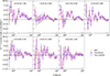 |
Fig. 10. Binned excess surface density-richness covariance in Eq. (38), as a function of the radius from the cluster center. We stack all clusters between λ ∈ [20, 70) and subdivide by different redshift bins from the top left panel to the bottom right panel. The true redshift case is displayed in pink, the BPZ and FlexZBoost cases are represented in orange and blue, respectively. |
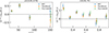 |
Fig. 11. Covariance in Eq. (38) modeled as a constant bias term bCov(M, z) across radius when binned by richness (left panel) or redshift (right panel). The positive covariance at large scales at lower redshift and richness bins is consistent with expectations from projection effects. |
To constrain the mass-richness relation while accounting for this effect, we modeled the stacked excess surface density profile using Eq. (35). We propagated the error of the shear-richness covariance (represented by the error bars in Figure 10) by adding the associated variance to the diagonal element of the total excess surface density profile covariance matrices, scaled by [log(10)β1/μm]2. We used the stacked profiles estimated with true background source redshifts and employed the inference setup defined in our baseline analysis, which involves a joint likelihood between counts and the stacked lensing profile. In Figure 12 (left panel), the filled (resp. dashed) contours show the posterior of the scaling relation parameters when accounting for (resp. not accounting for) the shear-richness covariance correction as calculated in Eq. (35). We observe that the “corrected” posterior is shifted by approximately 0.5σ compared to the baseline analysis. From this test, we find that the impact of property covariance significantly influences the scaling parameter inference. The size of this bias is larger than the one obtained using only FlexZBoost redshifts (see Sect. 5.3.1), but smaller than that from using only BPZ redshifts. Posterior shifts of roughly the same amplitude as the FlexZBoost-only (resp. BPZ-only) are obtained when using FlexZBoost (resp. BPZ) photometric source redshifts in addition to shear-richness covariance, as shown in the left panel of Figure 12. Finally, we show in the right panel of Figure 12 all sources of observational systematic effects that we tested in this work, namely the combination of (i) source photometric redshifts (either FlexZBoost or BPZ) (ii) the inclusion of the shear-richness covariance, and (iii) the addition of a free correcting photometric factor (1 + b) in the fit, to be compared with the baseline case (blue filled contours: true source redshift, and no shear-richness covariance).
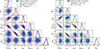 |
Fig. 12. Impact of shear-richness covariance on scaling relation parameter estimation. Left: Posterior distribution of the scaling relation parameters with (dashed blue) and without (filled blue) the shear-richness covariance correction in Eq. (35), considering true source galaxy redshifts. The red (resp. black) unfilled contours are obtained considering the shear-richness covariance and using FlexZBoost (resp. BPZ) photometric redshifts for source galaxies. Right: The blue filled contours are the same as in the left panel. The purple (resp. dashed green) unfilled contours are obtained considering the shear-richness covariance and using FlexZBoost (resp. BPZ) photometric redshifts, and letting the bias (1 + b) as a free parameter. These two effects explain somewhat the low amplitude (about 1 to 10%) of the shear-richness covariance (let us note that the ln(10)β1/μm factor in Eq. (35) is the order of unity; it does not change our conclusions). |
As mentioned above, the amplitude of the shear-richness covariance term is primarily influenced by the galaxy formation history within clusters and, secondarily, by the method used to populate halos in the simulation. As mentioned in Korytov et al. 2019, after defining the number of galaxies per halo, galaxy positions are drawn randomly in the halo environment (according to a generic NFW profile), thus not following the halo complex shape. As a result, the simulated shear-richness correlation is likely suppressed relative to what would be expected in real data. SkySim5000 Abolfathi et al. 2021, the extended version of cosmoDC2 covering 5000 deg2, features improved ray-tracing resolution and a more realistic model for galaxy population in halos. In particular, galaxies are distributed based on the triaxial configuration of halo dark matter particles, better capturing the underlying mass distribution. Leveraging SkySim5000 in future work will allow for a more realistic characterization of shear-richness covariance, especially at smaller scales and over a larger cluster sample.
Second, the shear-richness covariance also depends on the performance of the cluster finder. In our analysis, we used the redMaPPer cluster catalog derived from mock datasets, where the detection process is rather idealized compared to what would be expected from real observational data.
6. Summary and conclusions
We conducted several analyses based on the lensing profiles and abundance of redMaPPer-detected clusters in the DC2 simulation to constrain their mass-richness relation. We defined a baseline analysis, with state-of-the-art modeling choices and estimators. On this basis, we were able to test the impact of other modeling choices and observational systematics on the inferred mass-richness relation, also comparing it to a “fiducial” scaling relation. To do that, we used either stacked cluster lensing profiles or mean cluster lensing masses in combination with cluster count to explore several analysis setups: fixing or varying the cluster concentration, changing the dark matter density profile, adding shear-richness covariance.
6.1. Summary
For the various study cases explored in this paper, the best-fit values of the six-parameter redMaPPer mass-richness relation are summarized in Table E.1, with the corresponding study cases and their associated paper sections listed in Table 2.
In Figure 13, we illustrate the constraints on the three key parameters of the mean mass-richness relation defined in Eq. (16): lnλ0, μz, and μm. The vertical bands correspond to the fiducial constraints reported in Table 1, indicating the 1σ and 2σ confidence intervals. We first performed the analysis under ideal conditions, using the true shapes of background galaxies (i.e., their intrinsic ellipticities sheared by the local shear field) and their true redshifts. While the limited ray-tracing resolution of the DC2 simulation affects the innermost cluster regions (R < 1 Mpc), we found that combining cluster counts and lensing observables (whether via mean mass measurements or stacked profiles) yields tighter constraints on the scaling relation than using each probe independently. This improvement arises from the complementary degeneracy directions of the two observables. Using a NFW (Navarro et al. 1997) profile with the concentration-mass relation of Duffy et al. 2008, and restricting the radial fit to the one-halo regime (1 < R < 3.5 Mpc), we obtain constraints that are consistent at the 1σ level with the fiducial values derived from the match between redMaPPer clusters and dark matter halos. This consistency validates our joint count-and-lensing approach as a reliable method for constraining the mass-richness relation. We further tested the robustness of our results by varying the modeling assumptions of the stacked weak lensing profiles. In particular, we showed that the inferred posteriors are stable when adopting different concentration-mass relations, and remain consistent within 1σ with the results of the free-concentration case. Similarly, using alternative dark matter density profiles instead of NFW(e.g., Einasto or Hernquist) also offers robust and consistent constraints on the scaling relation parameters.
 |
Fig. 13. Constraints on the scaling relation parameters (only lnλ0, μz, and μm) obtained in Sect. 5. The vertical shaded region in each subplot represents the fiducial constraints presented in Sect. 3.4.1. For clarity, each color used for the plot corresponds to a subsection in Sect. 5. |
On the data side, we tested the impact of photometric redshift uncertainties on the inference of the mass-richness scaling relation by using outputs from two photometric redshift algorithms applied to cosmoDC2 galaxy magnitudes: BPZ Benítez 2011 and FlexZBoost Izbicki & Lee 2017. To accommodate the performance of each algorithm, we adapted the source galaxy selection accordingly. We found that FlexZBoost yields results that are fully consistent with the true-redshift case, indicating no significant bias. In contrast, the use of BPZ introduces a bias greater than 1σ in the normalization of the scaling relation. However, this bias can be mitigated by introducing a multiplicative correction factor, fitted jointly with the standard scaling relation parameters. In addition, we investigated the effect of shear-richness covariance, which arises from selection biases in the cluster-finding process. We found that within the radial range considered for fitting the cluster lensing profiles, the impact of covariance alone can shift μm by 0.5σ. This is comparable to the shift from the different c(M) models or using BPZ redshifts.
We complemented the summary plot by quantifying the level of tension between the results of various analyses and the fiducial constraints, as well as with respect to the baseline analysis. To this end, we employed the Gaussian tension metric Raveri & Doux 2021; Leizerovich et al. 2024, which expresses the tension between a Gaussian posterior, 𝒫, and a reference posterior, 𝒫fid, for a parameter θ in units of standard deviations. The tension is defined as
 (39)
(39)
where ⟨θ⟩𝒫 (resp. ⟨θ⟩𝒫fid) is the mean of the parameter posterior 𝒫(θ) (resp. 𝒫fid(θ)), and σ2(θ)𝒫 (resp. σ2(θ)𝒫fid) is the associated variance. For the different study cases, the level of tension with respect to the fiducial constraints (resp. the baseline case: weak lensing profiles combined with counts) is shown as circular dots (resp. star symbols) in Figure E.1. This approach allows us to quantitatively assess the Bayesian distance between the outcomes of various analysis setups and the fiducial model.
We find that combining probes (counts and lensing) does not significantly increase the level of tension, while it does enhance the statistical precision of the constraints. This demonstrates that our counts+lensing pipeline yields a consistent and reliable description of the observables. Furthermore, across all tested analysis configurations, the tension remains below the 2σ threshold. This highlights the robustness of our baseline analysis: variations in modeling assumptions or data choices result in posterior shifts that consistently stay within 2σ, underscoring the stability of the inferred scaling relation parameters.
6.2. Discussions and conclusions
To fully harness the cosmological constraining power of galaxy clusters, achieving a high level of precision on the cluster scaling relation is essential. This can be accomplished by jointly analyzing cluster counts and cluster weak gravitational lensing, enabling the inference of the mass-richness relation and its intrinsic scatter. For such analyses to be reliable, constraints from both lensing and counts must be robust against systematic effects. In this paper, we focus specifically on systematics related to cluster weak lensing.
In light of the first LSST data, we investigate the mass-richness relation of redMaPPer-detected galaxy clusters within the redshift range of 0.2 < z < 1 and richness range of 20 < λ < 200, using the DESC DC2 simulated dataset. We inferred a six-parameter log-normal cluster scaling relation, accounting for mass and redshift dependence in both the mean and scatter, via a joint analysis of stacked redMaPPer weak lensing profiles and cluster counts, thereby enhancing the overall constraining power. A series of robustness tests were performed, exploring the impact of cluster lensing profile modeling choices, photometric redshift uncertainties, and shear-richness covariance effects. We find that our constraints remain stable when lensing profiles are fitted in the one-halo regime (1 < R < 3.5 Mpc), assuming either true or photometric redshifts, and perfectly known source shapes. Furthermore, our results yield unbiased estimates of the fiducial redMaPPer mass-richness relation. While the constraining power in this analysis is limited compared to LSST expectations-to be  times larger – this work provides a solid foundation for scaling relation inference with future LSST cluster samples.
Moreover, the code work allows us to demonstrate the use of some of the software tools developed within DESC in concrete cluster analysis, representing a significant step in the calibration, validation, and methodological development. This paper thoroughly addresses all major systematics, except for shape measurement, which is discussed in detail below. The framework employed in this analysis is well integrated into the CLMM and CCL pipelines, paving the way for the development of cluster-based analyses in other official DESC pipeline codes such as TJPCov41 (official DESC covariance calculator interface), Firecrown42 (providing the DESC framework for implementing likelihoods and sampling parameters), and TXPipe43 (DESC library for summary statistics measurement, see Prat et al. 2023).
Due to the lack of ray-tracing resolution that motivated our conservative cut, we excluded the innermost regions, where the cluster lensing signal is the strongest. These scales are, however, crucial to enhancing the precision of weak lensing cluster masses. Analyzing such radial ranges requires a particular attention to modeling the dilution of the cluster lensing signal by member galaxies (contamination; see, e.g., Varga et al. 2019) and miscentering due to uncertainties in cluster finding methods Zhang et al. 2019; Köhlinger et al. 2015, which can be significant when referring to stacks of galaxy clusters.
Our analysis could benefit from further improvement to infer the redMaPPer cluster mass-richness relation. First, we considered the fiducial halo mass function of Despali et al. 2015, but propagating calibration uncertainties of this relation in our pipeline could have a non-negligible impact Artis et al. 2021; Kugel et al. 2025. Due to the noise level, we neglected the off-diagonal terms in the covariances of the stacked lensing profiles. However, rather close radial bins are known to be somewhat correlated due to the intrinsic variation of the halo density profile and large-scale structures Wu et al. 2019, which could degrade the precision of our results, even though they are much smaller than the galaxy shot and shape noise contribution.
Moreover, for the mean mass (two-step) approach, the link between the “true” mean mass of a stack and the inferred mean weak lensing mass may not be trivial Becker & Kravtsov 2011, contrary to what we used in Eq. (14), namely, a standard average mass over the redshift-richness cluster distribution. In reality, the excess surface density profile does not simply scale with the underlying cluster mass. For instance, Melchior et al. 2017 proposed a simple model where the excess surface density follows ΔΣ(R|M)∝MΓ(R|M) where Γ is the logarithmic slope of the excess surface density44; as a result, the mean weak lensing mass  has to be modeled by ∼⟨mΓ⟩1/Γ. Such non-linear dependence can be accounted for in the mean mass modeling in Eq. (14). Beyond this rather simple correction to link the mean lensing mass to the true average mass of the stack, McClintock et al. 2019 used simulations to reconstruct the stack lensing signal around clusters with masses drawn from the known P(M|λ) relation (as well as for concentrations and miscentering offsets drawn from specific distributions). They found that the bias between the true average mass and mean weak lensing mass may reach 10% (see their Figure 9) and has a strong richness and redshift dependence, indicating there a strong impact coming from the intrinsic scatter (in richness, concentration, miscentering, etc.).
Even though it is not sensitive to miscentering in our analysis (due to our restrictive low radial cut), we considered a fixed concentration-mass relation. However, it is known that cluster concentrations are scattered around a mean c(M) relation (see, e.g., Bullock et al. 2001; Darragh-Ford et al. 2023). This effect is particularly important in stacked analysis, especially at small radii. Accounting for this effect should degrade the precision of our obtained constraints by lowering the sensitivity of our model.
Finally, noise in galaxy shapes is one of the current main sources of scatter in weak lensing cluster mass estimation. First, as already mentioned earlier in this work, it originates from the intrinsic scatter of galaxy shapes, which is more and more mitigated by the increasing statistics of ongoing and future optical surveys. Second, it originates from the galaxy shape measurement algorithms, returning dispersed and biased estimations of intrinsic galaxy ellipticities. Shape reconstruction methods generally need to be calibrated from simulation or internally. Dispersed measured shapes as well as calibration uncertainties in these algorithms inevitably propagate to the cluster mass estimates, downgrading their precision. For that purpose, the DC2 object catalog Abolfathi et al. 2021 was built using the Rubin LSST science pipeline by identifying galaxies on cosmoDC2-based realistic images of the sky, including several realistic observational effects, such as atmospheric turbulence, telescope optics, and some detector effects. Several codes are used to measure shapes of detected galaxies, such as HSM Hirata & Seljak 2003; Mandelbaum et al. 2005 used on the HSC data Mandelbaum et al. 2018, and METACALIBRATION Sheldon & Huff 2017, used in the DES-Y3 cosmic shear analysis in Abbott et al. 2022. Ongoing efforts in DESC are aimed at studying the impact of galaxy detection and shape measurement in cluster fields on the accuracy and precision of cluster mass estimates (Ramel et al. in prep). These results will be essential to handling the full error budget on the mass-richness relation, in preparation for LSST cluster cosmology.
Especially on the total amount of matter in the Universe Ωm and the amplitude of matter fluctuations σ8.
Short for Röntgensatellit (in German X-rays are called Röntgenstrahlen).
Short for extended ROentgen Survey with an Imaging Telescope Array.
Here, we assume the survey depth is uniform across the sky.
Purity is generally defined as p(λ, zobs) instead of p(λ, z), where zobs is the cluster finder-inferred redshift. For simplicity, we consider here that observed and true redshifts (i.e., the redshift of the underlying dark matter halo) are equal.
The cluster center is typically identified from observational counterparts, such as the position of the brightest central galaxy. However, there may be an offset, called the miscentering radius, between the identified cluster center and the center of its gravitational potential.
The NFW profile, as well as other profiles used in the literature, are fitting functions calibrated on N-body simulations.
Such as low-mass galaxy halos, misidentified structures along the line of sight.
In the latter, we measure the cluster lensing profile for λ > 20, such as the redMaPPer purity is ∼99%.
Specifically, a very low-resolution internal dust model was used, which introduced artificial “breaks” in some galaxy spectra, especially at high redshift.
Template-fitting techniques are typically less affected by incomplete calibration data, but are more agnostic than empirical techniques, relying more on accurate SED modeling rather than the specificity of the calibration dataset.
This is not a fundamental limitation of template-fitting methods, but stems from the strong prior assumptions imposed by empirical techniques when generalizing p(z|m) from the calibration set to the LSST data.
In addition to redMaPPer, other cluster detection methods have been applied to the cosmoDC2 data, including WaZP Aguena et al. 2021a, AMICO Bellagamba et al. 2018, and YOLO-CL Grishin et al. 2023. The corresponding catalogs are currently available within DESC or are expected to be released soon.
Specifically, we use the redMaPPer member galaxies for each cluster (i.e., the output of redMaPPer), and the cosmoDC2 galaxies flagged as “members” for each cosmoDC2 dark matter halo in the simulation.
For z < 0.2 galaxies, the distinctive Balmer Break at 4000 Å falls in the u band.
To infer the intrinsic cosmoDC2 galaxy shape noise, we compute σSN = [stddev(ϵ1int)+stddev(ϵ2int)]/2, where  are the two components of the intrinsic galaxy ellipticities, identified as ellipticity_{1,2}_true in the cosmoDC2 catalog.
We adopted a redshift separation of Δz = 0.2 to mimic the common mitigation techniques of projection effects due to, e.g., contamination from foregrounds or cluster member galaxies. Additionally, since the lensing strength increases with the separation between the lens and the source, this threshold ensures that selected sources are more strongly lensed, thereby enhancing the S/N of the measurement. We do not explore less conservative cuts (e.g., Δz = 0.1 as in McClintock et al. 2019) in this work, as we expect them to have minimal impact on the results aside from increasing the per-cluster source galaxy number density, thereby enhancing the precision of the lensing measurement.
In Sect. 5, we give other methodologies considered for source selection when using photometric redshifts.
To go from stacked profile SNR to individual profile S/N, a good approximation is to rescale them by  .
.
Many parameterizations exist in the literature, such as the NFW profile Navarro et al. 1997, as well as those by Einasto 1965 and Hernquist 1990.
We use minuit.migrad() and minuit.minos() sequentially to (i) determine the best-fit mean cluster mass log10M and (ii) compute the asymmetric error bars log10M−σ−+σ+. In Eq. (27), we adopt a Gaussian likelihood with symmetric errors, for which we use the mean error (σ+ + σ−)/2. However, asymmetric errors can be more accurately modeled using, for example, a split normal distribution.
These modeling choices are referred to as the “baseline” analysis in the latter Section 5.1.
We discuss the upper radial cut R = 3.5 Mpc in Sect. 4.2.2, which is set to use only the 1-halo term lensing signal.
Wu et al. 2019 developed the cluster-lensing-cov package (https://github.com/hywu/cluster-lensing-cov), which provides analytical predictions for the excess surface density profile covariance.
The scale density is given by
 (31)
(31)
Again, we recall that the cosmological parameters are fixed to the DC2 values in the MCMC.
To compare joint constraints with abundance-alone or lensing-alone contours, we show in black in the left panel of Figure 6 the joint abundance and lensing profiles posterior.
The density ρ−2 is given by
![Mathematical equation: $$ \begin{aligned} \rho _{-2} = 200\rho _{c}(z)\frac{2}{3}\gamma ^{-1}\left[\frac{3}{\alpha }, \frac{2}{\alpha }c_{\rm 200c}^\alpha \right] \frac{c_{\rm 200c}^3}{e^{2/\alpha }} \left(\frac{2}{\alpha }\right)^{\frac{3-\alpha }{\alpha }}, \end{aligned} $$](/articles/aa/full_html/2025/08/aa54107-25/aa54107-25-eq64.gif) (33)
(33)
where γ is the lower incomplete gamma function.
Melchior et al. 2017 found a typical value of Γ = 0.74 for an NFW profile.
Acknowledgments
The authors thank the anonymous reviewer for their insightful comments and suggestions. This paper has undergone internal review by the LSST Dark Energy Science Collaboration. The authors thank the internal reviewers Tomomi Sunayama and Shenming Fu for their valuable comments. The authors thank Fabien Lacasa for useful discussions and for their help in using the PySSC code. The authors thank Dominique Boutigny for his help in using Qserv to access the cosmoDC2 simulated datasets at CC-IN2P3. CP conceptualized the project, developed the code, led the analysis, contributed to the paper’s structure and text, and oversaw the overall writing process. ZZ contributed to the shear-richness covariance analysis, the early development of the analysis framework and code, and the paper’s structure and text. MA developed the DESC matching library ClEvaR and contributed to the paper’s structure and text. CC assisted with project conceptualization and advising, participated in the early development and review of the analysis framework and code, and contributed to the paper’s structure and text. TG provided the parametrization of the redMaPPer selection function. MR prepared the matched cosmoDC2-redMaPPer catalog, reviewed various aspects of the analysis, and contributed to the paper’s structure and text. The remaining authors generated the data used in this work, contributed to the project’s infrastructure, and participated in discussions interpreting the results. The DESC acknowledges ongoing support from the Institut National de Physique Nucléaire et de Physique des Particules in France; the Science & Technology Facilities Council in the United Kingdom; and the Department of Energy and the LSST Discovery Alliance in the United States. DESC uses the resources of the IN2P3 Computing Center (CC-IN2P3–Lyon/Villeurbanne – France) funded by the Centre National de la Recherche Scientifique; the National Energy Research Scientific Computing Center, a DOE Office of Science User Facility supported by the Office of Science of the U.S. Department of Energy under Contract No. DE-AC02-05CH11231; STFC DiRAC HPC Facilities, funded by UK BEIS National E-infrastructure capital grants; and the UK particle physics grid, supported by the GridPP Collaboration. This work was performed in part under DOE Contract DE-AC02-76SF00515. MA is supported by the PRIN 2022 project EMC2 – Euclid Mission Cluster Cosmology: unlock the full cosmological utility of the Euclid photometric cluster catalog (code no. J53D23001620006). CA acknowledges support from DOE grant DE-SC0019193 and the Leinweber Center for Theoretical Physics. AF acknowledges support from the National Science Foundation under Cooperative Agreement 2421782 and the Simons Foundation award MPS-AI-00010515. We thank the developers and maintainers of the following software tools used in this work: NumPy van der Walt et al. 2011, SciPy Jones et al. 2001, Matplotlib Hunter 2007, GetDist Lewis 2019, emcee Foreman-Mackey et al. 2013, Astropy Astropy Collaboration 2013, Jupyter Kluyver et al. 2016.
References
- Abbott, T., Aguena, M., Alarcon, A., et al. 2022, Phys. Rev. D, 105, 023520 [NASA ADS] [CrossRef] [Google Scholar]
- Abdullah, M. H., Klypin, A., & Wilson, G. 2020, ApJ, 901, 90 [NASA ADS] [CrossRef] [Google Scholar]
- Abell, P. A., Allison, J., Anderson, S. F., et al. 2009, ArXiv e-prints [arXiv:0912.0201] [Google Scholar]
- Abolfathi, B., Alonso, D., Armstrong, R., et al. 2021, ApJS, 253, 31 [CrossRef] [Google Scholar]
- Aguena, M., & Lima, M. 2018, Phys. Rev. D, 98, 123529 [NASA ADS] [CrossRef] [Google Scholar]
- Aguena, M., Benoist, C., da Costa, L. N., et al. 2021a, MNRAS, 502, 4435 [NASA ADS] [CrossRef] [Google Scholar]
- Aguena, M., Avestruz, C., Combet, C., et al. 2021b, MNRAS, 508, 6092 [NASA ADS] [CrossRef] [Google Scholar]
- Aguena, M., Alves, O., Annis, J., et al. 2023, ArXiv e-prints [arXiv:2309.06593] [Google Scholar]
- Aihara, H., Armstrong, R., Bickerton, S., et al. 2018, PASJ, 70, S8 [NASA ADS] [Google Scholar]
- Allen, S. W., Evrard, A. E., & Mantz, A. B. 2011, ARA&A, 49, 409 [Google Scholar]
- Anbajagane, D., Evrard, A. E., Farahi, A., et al. 2020, MNRAS, 495, 686 [NASA ADS] [CrossRef] [Google Scholar]
- Artis, E., Melin, J.-B., Bartlett, J. G., & Murray, C. 2021, A&A, 649, A47 [NASA ADS] [CrossRef] [EDP Sciences] [Google Scholar]
- Astropy Collaboration 2013, A&A, 558, A33 [NASA ADS] [CrossRef] [EDP Sciences] [Google Scholar]
- Bartlett, J. G. 1997, ASP Conf. Ser., 126, 365 [Google Scholar]
- Baxter, E. J., Rozo, E., Jain, B., Rykoff, E., & Wechsler, R. H. 2016, MNRAS, 463, 205 [NASA ADS] [CrossRef] [Google Scholar]
- Becker, M. R., & Kravtsov, A. V. 2011, ApJ, 740, 25 [NASA ADS] [CrossRef] [Google Scholar]
- Bellagamba, F., Roncarelli, M., Maturi, M., & Moscardini, L. 2018, MNRAS, 473, 5221 [NASA ADS] [CrossRef] [Google Scholar]
- Benítez, N. 2011, Astrophysics Source Code Library [record ascl:1108.011] [Google Scholar]
- Benson, A. J. 2012, New Astron., 17, 175 [NASA ADS] [CrossRef] [Google Scholar]
- Bernstein, G. M., & Nakajima, R. 2009, ApJ, 693, 1508 [CrossRef] [Google Scholar]
- Bhattacharya, S., Habib, S., Heitmann, K., & Vikhlinin, A. 2013, ApJ, 766, 32 [Google Scholar]
- Binggeli, B. 1982, A&A, 107, 338 [NASA ADS] [Google Scholar]
- Bocquet, S., Grandis, S., Bleem, L. E., et al. 2024, Phys. Rev. D, 110, 083510 [NASA ADS] [CrossRef] [Google Scholar]
- Bulbul, E., Liu, A., Kluge, M., et al. 2024, A&A, 685, A106 [NASA ADS] [CrossRef] [EDP Sciences] [Google Scholar]
- Bullock, J. S., Kolatt, T. S., Sigad, Y., et al. 2001, MNRAS, 321, 559 [Google Scholar]
- Buote, D. A., & Lewis, A. D. 2004, ApJ, 604, 116 [Google Scholar]
- Chang, C., Jarvis, M., Jain, B., et al. 2013, MNRAS, 434, 2121 [NASA ADS] [CrossRef] [Google Scholar]
- Chen, K. F., Chiu, I. N., Oguri, M., et al. 2025, Open J. Astrophys., 8, 2 [Google Scholar]
- Chisari, N. E., Alonso, D., Krause, E., et al. 2019, ApJS, 242, 2 [Google Scholar]
- Chiu, I. N., Chen, K. F., Oguri, M., et al. 2024, Open J. Astrophys., 7, 90 [Google Scholar]
- Corless, V. L., & King, L. J. 2009, MNRAS, 396, 315 [Google Scholar]
- Costanzi, M., Rozo, E., Rykoff, E. S., et al. 2018, MNRAS, 482, 490 [Google Scholar]
- Costanzi, M., Rozo, E., Simet, M., et al. 2019, MNRAS, 488, 4779 [NASA ADS] [CrossRef] [Google Scholar]
- Cromer, D., Battaglia, N., Miyatake, H., & Simet, M. 2022, JCAP, 2022, 034 [CrossRef] [Google Scholar]
- Darragh-Ford, E., Mantz, A. B., Rasia, E., et al. 2023, MNRAS, 521, 790 [NASA ADS] [CrossRef] [Google Scholar]
- DES Collaboration 2020, Phys. Rev. D, 102, 023509 [NASA ADS] [CrossRef] [Google Scholar]
- DES Collaboration 2025, ArXiv e-prints [arXiv:2503.13632] [Google Scholar]
- Despali, G., Giocoli, C., & Tormen, G. 2014, MNRAS, 443, 3208 [Google Scholar]
- Despali, G., Giocoli, C., Angulo, R. E., et al. 2015, MNRAS, 456, 2486 [Google Scholar]
- Diemer, B., & Joyce, M. 2019, ApJ, 871, 168 [NASA ADS] [CrossRef] [Google Scholar]
- Diemer, B., & Kravtsov, A. V. 2014, ApJ, 789, 1 [NASA ADS] [CrossRef] [Google Scholar]
- Duffy, A. R., Schaye, J., Kay, S. T., & Dalla Vecchia, C. 2008, MNRAS, 390, L64 [Google Scholar]
- Einasto, J. 1965, Trudy Astrofizicheskogo Instituta Alma-Ata, 5, 87 [NASA ADS] [Google Scholar]
- Escoffier, S., Cousinou, M. C., Tilquin, A., et al. 2016, ArXiv e-prints [arXiv:1606.00233] [Google Scholar]
- Euclid Collaboration 2019, A&A, 627, A23 [NASA ADS] [CrossRef] [EDP Sciences] [Google Scholar]
- Evrard, A. E., Arnault, P., Huterer, D., & Farahi, A. 2014, MNRAS, 441, 3562 [CrossRef] [Google Scholar]
- Farahi, A., Evrard, A. E., Rozo, E., Rykoff, E. S., & Wechsler, R. H. 2016, MNRAS, 460, 3900 [NASA ADS] [CrossRef] [Google Scholar]
- Farahi, A., Evrard, A. E., McCarthy, I., Barnes, D. J., & Kay, S. T. 2018, MNRAS, 478, 2618 [NASA ADS] [CrossRef] [Google Scholar]
- Farahi, A., Anbajagane, D., & Evrard, A. E. 2022, ApJ, 931, 166 [Google Scholar]
- Foreman-Mackey, D., Hogg, D. W., Lang, D., & Goodman, J. 2013, PASP, 125, 306 [Google Scholar]
- Fumagalli, A., Saro, A., Borgani, S., et al. 2021, A&A, 652, A21 [NASA ADS] [CrossRef] [EDP Sciences] [Google Scholar]
- Fumagalli, A., Costanzi, M., Saro, A., Castro, T., & Borgani, S. 2024, A&A, 682, A148 [NASA ADS] [CrossRef] [EDP Sciences] [Google Scholar]
- Gao, L., Navarro, J. F., Cole, S., et al. 2008, MNRAS, 387, 536 [Google Scholar]
- Ghirardini, V., Bulbul, E., Artis, E., et al. 2024, A&A, 689, A298 [NASA ADS] [CrossRef] [EDP Sciences] [Google Scholar]
- Giocoli, C., Marulli, F., Moscardini, L., et al. 2021, A&A, 653, A19 [NASA ADS] [CrossRef] [EDP Sciences] [Google Scholar]
- Gouyou Beauchamps, S., Lacasa, F., Tutusaus, I., et al. 2022, A&A, 659, A128 [NASA ADS] [CrossRef] [EDP Sciences] [Google Scholar]
- Graham, M. L., Connolly, A. J., Ivezić, Z., et al. 2017, AJ, 155, 1 [Google Scholar]
- Grandis, S., Bocquet, S., Mohr, J. J., Klein, M., & Dolag, K. 2021, MNRAS, 507, 5671 [NASA ADS] [CrossRef] [Google Scholar]
- Grandis, S., Ghirardini, V., Bocquet, S., et al. 2024, A&A, 687, A178 [NASA ADS] [CrossRef] [EDP Sciences] [Google Scholar]
- Grishin, K., Mei, S., & Ilić, S. 2023, A&A, 677, A101 [NASA ADS] [CrossRef] [EDP Sciences] [Google Scholar]
- Gruen, D., Seitz, S., Becker, M. R., Friedrich, O., & Mana, A. 2015, MNRAS, 449, 4264 [NASA ADS] [CrossRef] [Google Scholar]
- Hasselfield, M., Hilton, M., Marriage, T. A., et al. 2013, JCAP, 2013, 008 [Google Scholar]
- Hearin, A., Korytov, D., Kovacs, E., et al. 2020, MNRAS, 495, 5040 [Google Scholar]
- Heitmann, K., Finkel, H., Pope, A., et al. 2019, ApJS, 245, 16 [NASA ADS] [CrossRef] [Google Scholar]
- Hernández-Martín, B., Schrabback, T., Hoekstra, H., et al. 2020, A&A, 640, A117 [EDP Sciences] [Google Scholar]
- Hernquist, L. 1990, ApJ, 356, 359 [Google Scholar]
- Hetterscheidt, M., Erben, T., Schneider, P., et al. 2005, A&A, 442, 43 [NASA ADS] [CrossRef] [EDP Sciences] [Google Scholar]
- Hirata, C., & Seljak, U. 2003, MNRAS, 343, 459 [Google Scholar]
- Hoekstra, H. 2003, MNRAS, 339, 1155 [NASA ADS] [CrossRef] [Google Scholar]
- Hogg, D. W. 1999, ArXiv e-prints [arXiv:astro-ph/9905116] [Google Scholar]
- Hu, W., & Kravtsov, A. V. 2003, ApJ, 584, 702 [Google Scholar]
- Hunter, J. D. 2007, Comput. Sci. Eng., 9, 90 [NASA ADS] [CrossRef] [Google Scholar]
- Izbicki, R., & Lee, A. B. 2017, ArXiv e-prints [arXiv:1704.08095] [Google Scholar]
- James, F., & Roos, M. 1975, Comput. Phys. Commun., 10, 343 [Google Scholar]
- Jimeno, P., Diego, J. M., Broadhurst, T., De Martino, I., & Lazkoz, R. 2018, MNRAS, 478, 638 [NASA ADS] [CrossRef] [Google Scholar]
- Jing, Y. P., & Suto, Y. 2002, ApJ, 574, 538 [Google Scholar]
- Jones, E., Oliphant, T., & Peterson, P. 2001, SciPy: Open Source Scientific Tools for Python [Google Scholar]
- Kaiser, N. 1984, ApJ, 284, L9 [NASA ADS] [CrossRef] [Google Scholar]
- Kluyver, T., Ragan-Kelley, B., Pérez, F., et al. 2016, Jupyter Notebooks-a publishing format for reproducible computational workflows (IOS Press), 87 [Google Scholar]
- Klypin, A., Yepes, G., Gottlöber, S., Prada, F., & Heß, S. 2016, MNRAS, 457, 4340 [Google Scholar]
- Köhlinger, F., Hoekstra, H., & Eriksen, M. 2015, MNRAS, 453, 3107 [NASA ADS] [Google Scholar]
- Komatsu, E., Dunkley, J., Nolta, M. R., et al. 2009, ApJS, 180, 330 [NASA ADS] [CrossRef] [Google Scholar]
- Komatsu, E., Smith, K. M., Dunkley, J., et al. 2011, ApJS, 192, 18 [Google Scholar]
- Korytov, D., Hearin, A., Kovacs, E., et al. 2019, ApJS, 245, 26 [NASA ADS] [CrossRef] [Google Scholar]
- Kovacs, E., Mao, Y.-Y., Aguena, M., et al. 2022, OJAp, 5, 1 [Google Scholar]
- Kravtsov, A. V., & Borgani, S. 2012, ARA&A, 50, 353 [Google Scholar]
- Kugel, R., Schaye, J., Schaller, M., Forouhar Moreno, V. J., & McGibbon, R. J. 2025, MNRAS, 537, 2179 [Google Scholar]
- Lacasa, F., Lima, M., & Aguena, M. 2018, A&A, 611, A83 [NASA ADS] [CrossRef] [EDP Sciences] [Google Scholar]
- Laureijs, R., Amiaux, J., Arduini, S., et al. 2011, ArXiv e-prints [arXiv:1110.3193] [Google Scholar]
- Lee, B. E., Le Brun, A. M. C., Haq, M. E., et al. 2018, MNRAS, 479, 890 [Google Scholar]
- Lee, A., Wu, H. Y., Salcedo, A. N., et al. 2024, Phys. Rev. D, 111, 063502 [Google Scholar]
- Leizerovich, M., Landau, S. J., & Scóccola, C. G. 2024, Phys. Lett. B, 855, 138844 [Google Scholar]
- Lesci, G. F., Marulli, F., Moscardini, L., et al. 2022, A&A, 659, A88 [NASA ADS] [CrossRef] [EDP Sciences] [Google Scholar]
- Lewis, A. 2019, ArXiv e-prints [arXiv:1910.13970] [Google Scholar]
- LSST Dark Energy Science Collaboration 2012, ArXiv e-prints [arXiv:1211.0310] [Google Scholar]
- Mandelbaum, R., Hirata, C. M., Seljak, U., et al. 2005, MNRAS, 361, 1287 [Google Scholar]
- Mandelbaum, R., Lanusse, F., Leauthaud, A., et al. 2018, MNRAS, 481, 3170 [NASA ADS] [CrossRef] [Google Scholar]
- Mantz, A. B. 2019, MNRAS, 485, 4863 [NASA ADS] [CrossRef] [Google Scholar]
- Mantz, A., Allen, S. W., Ebeling, H., & Rapetti, D. 2008, MNRAS, 387, 1179 [CrossRef] [Google Scholar]
- Mantz, A. B., von der Linden, A., Allen, S. W., et al. 2015, MNRAS, 446, 2205 [Google Scholar]
- McClintock, T., Varga, T. N., Gruen, D., et al. 2019, MNRAS, 482, 1352 [Google Scholar]
- Melchior, P., Gruen, D., McClintock, T., et al. 2017, MNRAS, 469, 4899 [CrossRef] [Google Scholar]
- Mistele, T., & Durakovic, A. 2024, Open J. Astrophys., 7, 120 [Google Scholar]
- Mulroy, S. L., Farahi, A., Evrard, A. E., et al. 2019, MNRAS, 484, 60 [NASA ADS] [CrossRef] [Google Scholar]
- Murata, R., Oguri, M., Nishimichi, T., et al. 2019, PASJ, 71, 107 [CrossRef] [Google Scholar]
- Murray, C., Bartlett, J. G., Artis, E., & Melin, J.-B. 2022, MNRAS, 512, 4785 [NASA ADS] [CrossRef] [Google Scholar]
- Myles, J., Gruen, D., Mantz, A. B., et al. 2021, MNRAS, 505, 33 [NASA ADS] [CrossRef] [Google Scholar]
- Myles, J., Gruen, D., Jeltema, T., et al. 2025, ArXiv e-prints [arXiv:2506.06249] [Google Scholar]
- Navarro, J. F., Frenk, C. S., & White, S. D. M. 1997, ApJ, 490, 493 [Google Scholar]
- Nord, B., Stanek, R., Rasia, E., & Evrard, A. E. 2008, MNRAS, 383, L10 [Google Scholar]
- Oguri, M., & Takada, M. 2011, Phys. Rev., D, 83 [Google Scholar]
- Oguri, M., Lee, J., & Suto, Y. 2003, ApJ, 599, 7 [NASA ADS] [CrossRef] [Google Scholar]
- Oguri, M., Takada, M., Okabe, N., & Smith, G. P. 2010, MNRAS, 402, 307 [NASA ADS] [CrossRef] [Google Scholar]
- Pacaud, F., Pierre, M., Melin, J.-B., et al. 2018, A&A, 620, A10 [NASA ADS] [CrossRef] [EDP Sciences] [Google Scholar]
- Park, Y., Sunayama, T., Takada, M., et al. 2023, MNRAS, 518, 5171 [Google Scholar]
- Parroni, C., Mei, S., Erben, T., et al. 2017, ApJ, 848, 114 [Google Scholar]
- Payerne, C., Murray, C., Combet, C., et al. 2023, MNRAS, 520, 6223 [NASA ADS] [CrossRef] [Google Scholar]
- Payerne, C., Murray, C., Combet, C., & Penna-Lima, M. 2024, MNRAS, 532, 381 [Google Scholar]
- Phriksee, A., Jullo, E., Limousin, M., et al. 2020, MNRAS, 491, 1643 [NASA ADS] [CrossRef] [Google Scholar]
- Planck Collaboration XX. 2014, A&A, 571, A20 [NASA ADS] [CrossRef] [EDP Sciences] [Google Scholar]
- Planck Collaboration XXIV. 2016, A&A, 594, A24 [NASA ADS] [CrossRef] [EDP Sciences] [Google Scholar]
- Planck Collaboration XXVII. 2016, A&A, 594, A27 [NASA ADS] [CrossRef] [EDP Sciences] [Google Scholar]
- Poisson, S. D. 1837, Bachelier, Imprimeur-Librairie [Google Scholar]
- Prada, F., Klypin, A. A., Cuesta, A. J., Betancort-Rijo, J. E., & Primack, J. 2012, MNRAS, 423, 3018 [NASA ADS] [CrossRef] [Google Scholar]
- Pranjal, R. S., Krause, E., Huang, H.-J., et al. 2023, MNRAS, 524, 3324 [Google Scholar]
- Prat, J., Zuntz, J., Chang, C., et al. 2023, Open J. Astrophys., 6, 13 [Google Scholar]
- Pratt, G. W., Arnaud, M., Biviano, A., et al. 2019, Space Sci. Rev., 215, 25 [Google Scholar]
- Raveri, M., & Doux, C. 2021, Phys. Rev. D, 104, 043504 [NASA ADS] [CrossRef] [Google Scholar]
- Rozo, E., Evrard, A. E., Rykoff, E. S., & Bartlett, J. G. 2014, MNRAS, 438, 62 [Google Scholar]
- Rykoff, E. S., Rozo, E., Busha, M. T., et al. 2014, ApJ, 785, 104 [Google Scholar]
- Rykoff, E. S., Rozo, E., Hollowood, D., et al. 2016, ApJS, 224, 1 [NASA ADS] [CrossRef] [Google Scholar]
- Sadibekova, T., Pierre, M., Clerc, N., et al. 2014, A&A, 571, A87 [NASA ADS] [CrossRef] [EDP Sciences] [Google Scholar]
- Sanderson, A. J. R., & Ponman, T. J. 2009, MNRAS, 402, 65 [Google Scholar]
- Saro, A., Bocquet, S., Rozo, E., et al. 2015, MNRAS, 454, 2305 [Google Scholar]
- Schmidt, S. J., Malz, A. I., Soo, J. Y. H., et al. 2020, MNRAS, 499, 1587 [Google Scholar]
- Schneider, P., Ehlers, J., & Falco, E. E. 1992, Gravitational Lenses [Google Scholar]
- Schneider, M. D., Frenk, C. S., & Cole, S. 2012, JCAP, 2012, 030 [CrossRef] [Google Scholar]
- Sereno, M., Fedeli, C., & Moscardini, L. 2016, JCAP, 2016, 042 [NASA ADS] [CrossRef] [Google Scholar]
- Sheldon, E. S., & Huff, E. M. 2017, ApJ, 841, 24 [NASA ADS] [CrossRef] [Google Scholar]
- Sheldon, E. S., Johnston, D. E., Frieman, J. A., et al. 2004, AJ, 127, 2544 [Google Scholar]
- Sheth, R. K., Mo, H. J., & Tormen, G. 2001, MNRAS, 323, 1 [NASA ADS] [CrossRef] [Google Scholar]
- Shirasaki, M., & Takada, M. 2018, MNRAS, 478, 4277 [Google Scholar]
- Simet, M., McClintock, T., Mandelbaum, R., et al. 2017, MNRAS, 466, 3103 [NASA ADS] [CrossRef] [Google Scholar]
- Sommer, M. W., Schrabback, T., Applegate, D. E., et al. 2022, MNRAS, 509, 1127 [Google Scholar]
- Spergel, D., Gehrels, N., Baltay, C., et al. 2015, ArXiv e-prints [arXiv:1503.03757] [Google Scholar]
- Sunayama, T., Park, Y., Takada, M., et al. 2020, MNRAS, 496, 4468 [CrossRef] [Google Scholar]
- Sunayama, T., Miyatake, H., Sugiyama, S., et al. 2024, Phys. Rev. D, 110, 083511 [NASA ADS] [Google Scholar]
- Tinker, J. L., Robertson, B. E., Kravtsov, A. V., et al. 2010, ApJ, 724, 878 [NASA ADS] [CrossRef] [Google Scholar]
- Umetsu, K. 2020, A&ARv, 28 [Google Scholar]
- van der Walt, S., Colbert, S. C., & Varoquaux, G. 2011, Comput. Sci. Eng., 13, 22 [Google Scholar]
- Varga, T. N., DeRose, J., Gruen, D., et al. 2019, MNRAS, 489, 2511 [NASA ADS] [CrossRef] [Google Scholar]
- Vogt, S. M. L., Bocquet, S., Davies, C. T., et al. 2024, Phys. Rev. D, 111, 043519 [Google Scholar]
- Wang, J., Bose, S., Frenk, C. S., et al. 2020, Nature, 585, 39 [Google Scholar]
- Wright, A. H., Hildebrandt, H., van den Busch, J. L., & Heymans, C. 2020, A&A, 637, A100 [NASA ADS] [CrossRef] [EDP Sciences] [Google Scholar]
- Wu, H.-Y., Weinberg, D. H., Salcedo, A. N., Wibking, B. D., & Zu, Y. 2019, MNRAS, 490, 2606 [Google Scholar]
- Wu, H.-Y., Costanzi, M., To, C.-H., et al. 2022, MNRAS, 515, 4471 [CrossRef] [Google Scholar]
- Zhang, Y., Jeltema, T., Hollowood, D. L., et al. 2019, MNRAS, 487, 2578 [NASA ADS] [CrossRef] [Google Scholar]
- Zhang, Z., Wu, H.-Y., Zhang, Y., et al. 2023, MNRAS, 523, 1994 [Google Scholar]
- Zhang, Z., Farahi, A., Nagai, D., et al. 2024, MNRAS, [arXiv:2310.18266] [Google Scholar]
- Zhou, C., Wu, H.-Y., Salcedo, A. N., et al. 2024, Phys. Rev. D, 110, 103508 [Google Scholar]
- Zwicky, F. 1937, ApJ, 86, 217 [NASA ADS] [CrossRef] [Google Scholar]
Appendix A: Stability of the fiducial cluster scaling relation
The fiducial scaling relation used throughout this paper was derived from the matched catalog between redMaPPer clusters and cosmoDC2 halos, restricted to λ > 5 and M200c > 1013 M⊙. In this appendix, we detail the various selection cuts applied to the matched catalog before inferring the fiducial relation using the likelihood defined in Eq. (18). For illustration, the posterior distributions of the mean scaling relation parameters, obtained using the matched catalog before applying any richness or mass cuts, are shown as green unfilled contours in Figure A.1.
Initially, we assume that the matched catalog is unaffected by the purity of the redMaPPer cluster finder, as false detections have been excluded after matching. However, the completeness of redMaPPer still impacts the catalog, particularly at the low-mass end where some halos are not detected. Ideally, the likelihood in Eq. (18) should account for such missing halos. To partially mitigate this effect, we apply a lower mass cut of M200c > 4 × 10¹³ M⊙, a regime where redMaPPer’s completeness exceeds 50%. The resulting posterior, reflecting this correction, is shown as magenta unfilled contours in Figure A.1.
Additionally, our cluster scaling relation model in Eq. (15) does not account for Poisson noise in redMaPPer richness determination. This noise can be incorporated by revising Eq. (15):
 (A.1)
(A.1)
where 𝒫(λ|λint) is the Poisson distribution, and P(λint|m, z) represents the probability density function for the intrinsic richness, which can be expressed with the same equation as in Eq. (15), but with intrinsic variance only. This updated P(λ|m, z) can be approximated by using the same P(λint|m, z) while updating the variance by
![Mathematical equation: $$ \begin{aligned} \sigma _{\ln \lambda |m,z}^2 \approx [\sigma _{\ln \lambda |m,z}]_{\rm int}^2 + \frac{\exp (\langle \ln \lambda |m,z\rangle )-1}{\exp (2\langle \ln \lambda |m,z\rangle )}, \end{aligned} $$](/articles/aa/full_html/2025/08/aa54107-25/aa54107-25-eq66.gif) (A.2)
(A.2)
where [σlnλ|m, z]int2 is provided in Eq. (17), now only describing the intrinsic variance of richness. The impact of the Poisson noise, represented by the second term (see, e.g., Zhang et al. 2023), diminishes for large richness. Consequently, we apply a low richness cut λ > 10 to align with the Poisson-free distribution in Eq. (15).
Combining this with the mass cut M200c > 4 × 10¹³ M⊙, the constraints are identified as our fiducial choice. We observe that the three fiducial constraints agree within < 2σ of the baseline count+weak lensing posteriors. We also explore a stricter cut, λ > 20, combined with M200c > 4 × 10¹³ M⊙. This λ > 20 scenario results in larger error bars (still compatible with count+weak lensing constraints) but biases the mass slope μm lower than other choices. In fact, from the left panel in Figure 1, the λ > 20 cut over-weights high-richness clusters in the fiducial fit, even after correcting the distribution P(λ|m, z) using a truncated Gaussian to account for the minimum richness. While we adopted the black dashed contours as our fiducial constraints, further investigations are warranted.
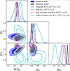 |
Fig. A.1. Posterior distribution of the mean scaling relation parameters from our count+lensing baselines (filled contours) and the matched redMaPPer-cosmoDC2 cluster-halo match catalog, for different richness and mass cuts. |
Appendix B: Impact of the radial fitting range on the scaling relation parameters
In this appendix we test the impact of the fitting radial range [1, Rmax] of the stacked excess surface density profiles on the scaling relation parameters. Our baseline adopts a conservative choice of Rmax = 3.5 Mpc for fitting the stacked excess surface density profiles, ensuring sensitivity to the one-halo regime only. At larger radii, the influence of the two-halo term is expected to become more significant, and modeling the stacked profiles using only the one-halo regime may be insufficient. From Oguri & Takada 2011, the two-halo excess surface density is given by
 (B.1)
(B.1)
where kl = l/[DA(z)(1 + z)], J2 is the second order Bessel function of the first kind, θ = R/DA(z) is the separation angle, ρm(z) is the matter density at redshift z, bh(M, z) is the halo bias at mass M and redshift z and Pm(k, z) is the matter power spectrum at the halo redshift z. Finally, the total excess surface density profile is given by
 (B.2)
(B.2)
We repeated the scaling relation parameter fit using Rmax = 5.5 and Rmax = 10 Mpc, respectively. The mean scaling relation parameters for these different fitting radial ranges are shown in Figure B.1. Both new cuts yield conclusions consistent with the baseline, with shifts of less than < 1σ compared to the baseline constraints.
Interestingly, the results for Rmax = 10 Mpc are close to the baseline constraints, despite the absence of modeling for the two-halo term in the stacked lensing profile. We attribute this to the lower S/N of measurements at large scales, which reduces the impact of the two-halo term. However, with larger datasets, the two-halo term must be accurately modeled beyond R = 4 Mpc Murata et al. 2019; McClintock et al. 2019; Melchior et al. 2017.
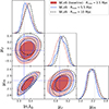 |
Fig. B.1. Posterior distribution of the mean scaling relation parameters from the combination of count and lensing profiles, for three different values of Rmax, used in the stacked lensing profile fitting range [1, Rmax]. |
Appendix C: Some other observational systematics
C.1. Miscentering
When the inferred cluster center differs from the one of its underlying halo’s gravitational potential – which happens when deriving the cluster center from the intra-cluster galaxy distribution – the lensing profile modeling must account for a miscentering term. For a single miscentered cluster with offset radius Rmis, its radially averaged projected mass density is given by
 (C.1)
(C.1)
For a stack of clusters, the above equation can be averaged over the distribution of miscentering P(Rmis), such as
 (C.2)
(C.2)
From this equation, we can obtain ΔΣmis by injecting it into Eq. (10). The total one-halo term depends on the fraction fmis of miscentered clusters, as shown in, for example, Giocoli et al. 2021, and is given by
 (C.3)
(C.3)
where ΔΣ1h, cen(R) denotes the lensing profile of a perfectly centered stack of clusters. To test the impact of miscentering of redMaPPer clusters, we use the matched catalog between redMaPPer clusters and cosmoDC2 dark matter halos obtained in Sect. 3.4. In each cluster-halo pair, we consider the halo-member galaxy flagged as is_central==True in the cosmoDC2 extragalactic catalog to trace the center of the halo’s gravitational potential, from which we compute the corresponding projected offset radius Rmis of the matched redMaPPer cluster. We found that the fraction of perfectly centered clusters (for which Rmis = 0) is 85% so fmis = 0.15. For pairs with Rmis ≠ 0, the distribution of offsets between cosmoDC2 halo and redMaPPer cluster centers is well described by a Gamma distribution McClintock et al. 2019 given by
 (C.4)
(C.4)
with σmis = 0.12 Mpc. We use the cluster_toolkit package45 to compute the miscentered profile evoked in Sect. 2 over a wide range of mass and redshift, and we found that the bias compared to a perfectly centered profile is at most 1% at R = 1 Mpc, and 0.25% at R = 2 Mpc. For simplicity, since the computation of the miscentering term is computationally demanding, we chose to neglect this contribution.
C.2. Contamination
The background source selection may cause contamination of the source sample by cluster member galaxies Varga et al. 2019, which dilutes the signal in the innermost region. The observed contaminated lensing profile accounting for this dilution is given by
![Mathematical equation: $$ \begin{aligned} \Delta \Sigma _{ij}^\mathrm{cont}(R) = [1-f_{\rm cl}(R)]\Delta \Sigma _{ij}(R), \end{aligned} $$](/articles/aa/full_html/2025/08/aa54107-25/aa54107-25-eq73.gif) (C.5)
(C.5)
where ΔΣij(R) is given in Eq. (13), fcl(R) is the fraction of "source-selected" member galaxies at a distance R from the cluster center, and is a decreasing function of R. At fixed R, the fraction fcl increases with mass, since massive clusters have more member galaxies, and thus are more subject to this effect Varga et al. 2019.
For each redMaPPer cluster, we consider the corresponding matched dark matter halo in the matched catalog presented in Sect. 3. We applied the photo-z source selection and then identified the remaining halo "member galaxies," as labeled in the simulation (which are randomly drawn at the HOD level in the DC2 workflow to populate halos, see Korytov et al. 2019). This procedure enables us to recover fcl(R) for a variety of masses and redshifts, and we found that the correcting factor [1 − fcl(R = 1 Mpc)] ∼ 1 after combining the two cuts, and for both BPZ and FlexZBoost algorithms. We find that our source selection enables us to discriminate efficiently between true sources and member galaxies (the effect is less than 0.1%).
Appendix D: Derivation of the selection bias
In this appendix we use the notation
 (D.1)
(D.1)
We can consider that the measured shear and richness are correlated, such that they can be modeled as correlated random variables via P(ΔΣ, λ|m). Then, the average excess surface density profile within the i-th redshift bin and the j-th richness bin is given by
 (D.2)
(D.2)
From Wu et al. 2022, we consider P(ΔΣ, λ|m) as a multivariate Gaussian distribution, with means ⟨ΔΣ|m, z⟩ and ⟨lnλ|m, z⟩, and with covariance matrix
 (D.3)
(D.3)
From Wu et al. 2019 (see their Eq. 8), the conditional mean of ΔΣ is given by
![Mathematical equation: $$ \begin{aligned} \langle \Delta \Sigma |m, \lambda , z \rangle = \langle \Delta \Sigma |m, z \rangle + r\frac{\sigma _{\Delta \Sigma }}{\sigma _{\ln \lambda }}[\ln \lambda - \langle \ln \lambda |m, z\rangle ]. \end{aligned} $$](/articles/aa/full_html/2025/08/aa54107-25/aa54107-25-eq77.gif) (D.4)
(D.4)
From Farahi et al. 2022, we can approximate the halo mass function to the form
![Mathematical equation: $$ \begin{aligned} N(m,z) \approx A(z) \exp \left[- \beta _1 \ln m \right]. \end{aligned} $$](/articles/aa/full_html/2025/08/aa54107-25/aa54107-25-eq78.gif) (D.5)
(D.5)
By using the simplified mean mass-richness relation,
 (D.6)
(D.6)
where  is linked to the μm in Eq. (16) by
  , and the results in Evrard et al. 2014 (see their Eq. 3 and 4), we have
 (D.7)
(D.7)
Using that  Evrard et al. 2014, we have
 (D.8)
(D.8)
So, by combining Eq. (D.4) and Eq. (D.8), we get
 (D.9)
(D.9)
 (D.10)
From above, we find that the stacked shear decomposes as ⟨ΔΣ⟩=⟨ΔΣ⟩1 + ⟨ΔΣ⟩2 + ⟨ΔΣ⟩3. The first term is given by
 (D.11)
The second term is given by
 (D.12)
 (D.13)
 (D.14)
where the second equation is obtained by considering that Cov(ΔΣ, lnλ|m, z) evolves linearly with mass m. The term ⟨ΔΣ⟩3 is negligible and not considered in this analysis (see, e.g., Wu et al. 2022; Zhang et al. 2024). Then, from the above equation, we see that a possible shear-richness correlation (e.g., r ≠ 0, or equivalently Cov(ΔΣ, lnλ|m, z)≠0), arising from selection bias in cluster finder algorithms, may lead to a misinterpretation of the stacked cluster profile as a naive average as given in Eq. (D.11).
Appendix E: Constraints of the scaling relation: Summary table
We list in
Table E.1 the values of the scaling relation parameters obtained from cluster count and/or cluster lensing in Sect. 5.1 (baseline analysis), Sect. 5.2.1 (impact of c(M) relation), Sect. 5.2.2 (impact of density profile), Sect. 5.3.1 (impact of source galaxy photometric redshifts), and Sect. 5.3.2 (impact of shear-richness covariance). The Figure E.1 displays the tension metric for the different study cases with respect to (i) the fiducial constraints and (ii) the count+weak lensing profiles analysis, labeled as the "baseline" in Sect. 5.1.
Best-fit parameters of the cluster scaling relation in Eq. (15).
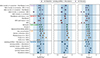 |
Fig. E.1. Tension in numbers of σ between the different count and/or lensing analyses and the fiducial constraints (circle dots) for the parameters listed in Figure 13, and between the different analyses and the baseline weak lensing and count analysis (star dots). |
All Tables
Fiducial values of the parameters of the redMaPPer cluster mass-richness relation.
All Figures
|
Fig. 1. Left: cosmoDC2 halo M200c masses (from the simulation) versus the redMaPPer cluster richnesses. The points are colored with the redMaPPer cluster redshift. The solid line is the best-fitted mean richness-mass relation in Eq. (16) at z = 0.4. The dashed lines represent the low mass and low richness cut used on the cosmoDC2-redMaPPer matched catalog for the fit of the fiducial scaling relation. Right: Histogram of richnesses in bins of mass, and best-fit probability distributions P(lnλ|M, z) from Eq. (15) (solid lines) for the different mass bins. |
| In the text | |
|
Fig. 2. Measured count of redMaPPer cluster as a function of richness, for different richness bins. For each richness-redshift bin, the width of the shaded area represent the width of the richness bin, and the height correspond to the Poisson noise |
| In the text | |
|
Fig. 3. Stacked excess surface density profile as a function of the distance to the cluster center, for different richness bins (colors) and different redshift bins (from top left to bottom right). The error bars are the diagonal elements of the bootstrap covariance matrices. The dashed black vertical line (resp. black filled vertical line) represents the R > 1 Mpc cut (resp. R < 3.5 Mpc cut). |
| In the text | |
|
Fig. 4. S/Ns of the stacked excess surface density profiles, for two different richness bins (left and right panel) and different richness bins (colors). |
| In the text | |
|
Fig. 5. Left: Mean cluster lensing mass as a function of mean richness within the stack, the different colors correspond to the different redshift bins. Right: Mean cluster lensing masses as a function of the DC2 matched masses from the cosmoDC2 dark matter halo catalog. The different colors correspond to the different redshift bins. The dashed line corresponds to y = x. |
| In the text | |
|
Fig. 6. Left: Posterior distribution of the scaling relation parameters using abundance alone (blue), lensing profiles alone (dashed red), or masses alone (solid green lines). The joint abundance and lensing profiles posterior is displayed in black. Right: Posterior distribution of scaling relation parameters when combining abundance and lensing profiles (solid blue lines) and combining abundance and cluster masses (orange-filled contours). The dashed contours are obtained by removing the last redshift bin for both abundance and lensing. |
| In the text | |
|
Fig. 7. Left: Posterior distribution of the scaling relation parameters using count/mass likelihood. The concentration-free case is shown with the dashed lines, the other contours are obtained using various concentration-mass relations from the literature. Right: Posterior distribution of the scaling relation parameters using count/mass likelihood, without using a concentration-mass relation, and using different modeling of the cluster density profile, namely NFW (red filled contours), Einasto (solid lines), and Hernquist (dashed lines). |
| In the text | |
|
Fig. 8. Left: Mean photometric redshift against true cosmoDC2 redshift for BPZ and FlexZBoost methods. Right: Distribution of true cosmoDC2 redshifts after our magnitude cuts (black). Upper panel: The blue distribution represents the same distribution after a cut on the probability P(zs > zl) using FlexZBoost photometric redshift, for a cluster at z = 0.38. The orange distribution is obtained after combining the P(zs > zl) cut and the mean redshift cut. Lower panel: Same as upper panel but for BPZ redshifts. On both panels, the vertical red line indicates the position of the cluster redshift. |
| In the text | |
|
Fig. 9. Impact of photometric redshifts of source galaxies on scaling relation parameter estimation. Left: The filled contours show the constraints when using true redshifts of source galaxies. Dashed contours are obtained when considering the BPZ photometric redshifts. Empty contours are obtained using BPZ photometric redshifts, after marginalizing over the (1 + b) correcting factor, considered as a free parameter, used to correct from photometric redshift calibration issues. Right: same as left panel, but for FlexZBoost. |
| In the text | |
|
Fig. 10. Binned excess surface density-richness covariance in Eq. (38), as a function of the radius from the cluster center. We stack all clusters between λ ∈ [20, 70) and subdivide by different redshift bins from the top left panel to the bottom right panel. The true redshift case is displayed in pink, the BPZ and FlexZBoost cases are represented in orange and blue, respectively. |
| In the text | |
|
Fig. 11. Covariance in Eq. (38) modeled as a constant bias term bCov(M, z) across radius when binned by richness (left panel) or redshift (right panel). The positive covariance at large scales at lower redshift and richness bins is consistent with expectations from projection effects. |
| In the text | |
|
Fig. 12. Impact of shear-richness covariance on scaling relation parameter estimation. Left: Posterior distribution of the scaling relation parameters with (dashed blue) and without (filled blue) the shear-richness covariance correction in Eq. (35), considering true source galaxy redshifts. The red (resp. black) unfilled contours are obtained considering the shear-richness covariance and using FlexZBoost (resp. BPZ) photometric redshifts for source galaxies. Right: The blue filled contours are the same as in the left panel. The purple (resp. dashed green) unfilled contours are obtained considering the shear-richness covariance and using FlexZBoost (resp. BPZ) photometric redshifts, and letting the bias (1 + b) as a free parameter. These two effects explain somewhat the low amplitude (about 1 to 10%) of the shear-richness covariance (let us note that the ln(10)β1/μm factor in Eq. (35) is the order of unity; it does not change our conclusions). |
| In the text | |
|
Fig. 13. Constraints on the scaling relation parameters (only lnλ0, μz, and μm) obtained in Sect. 5. The vertical shaded region in each subplot represents the fiducial constraints presented in Sect. 3.4.1. For clarity, each color used for the plot corresponds to a subsection in Sect. 5. |
| In the text | |
|
Fig. A.1. Posterior distribution of the mean scaling relation parameters from our count+lensing baselines (filled contours) and the matched redMaPPer-cosmoDC2 cluster-halo match catalog, for different richness and mass cuts. |
| In the text | |
|
Fig. B.1. Posterior distribution of the mean scaling relation parameters from the combination of count and lensing profiles, for three different values of Rmax, used in the stacked lensing profile fitting range [1, Rmax]. |
| In the text | |
|
Fig. E.1. Tension in numbers of σ between the different count and/or lensing analyses and the fiducial constraints (circle dots) for the parameters listed in Figure 13, and between the different analyses and the baseline weak lensing and count analysis (star dots). |
| In the text | |
Current usage metrics show cumulative count of Article Views (full-text article views including HTML views, PDF and ePub downloads, according to the available data) and Abstracts Views on Vision4Press platform.
Data correspond to usage on the plateform after 2015. The current usage metrics is available 48-96 hours after online publication and is updated daily on week days.
Initial download of the metrics may take a while.