| Issue |
A&A
Volume 700, August 2025
|
|
|---|---|---|
| Article Number | A262 | |
| Number of page(s) | 11 | |
| Section | Interstellar and circumstellar matter | |
| DOI | https://doi.org/10.1051/0004-6361/202554135 | |
| Published online | 26 August 2025 | |
The Snake filament: A study of polarization and kinematics
1
Centre for Astrochemical Studies, Max-Planck-Institut für extraterrestrische Physik,
Gießenbachstraße1,
85748
Garching bei München,
Germany
2
European Southern Observatory,
Karl-Schwarzschild-Straße 2,
85748
Garching bei München,
Germany
3
Departamento de Física–ICEx–UFMG,
Caixa Postal 702,
30.123-970
Belo Horizonte,
Brazil
★ Corresponding author.
Received:
14
February
2025
Accepted:
10
July
2025
Abstract
Context. Understanding the role of magnetic fields in the formation of dense filamentary structures in molecular clouds is critical for understanding the star formation process. The Snake filament, which is in or close to the Pipe Nebula’s neighborhood, is a prominent example of such structures and offers an ideal environment to study the interplay between magnetic fields and gas dynamics in the early stages of star formation.
Aims. We investigated how magnetic fields influence the structure and dynamics of the Snake filament using both polarization data and molecular line observations. Our goal is to understand the role of magnetic fields in shaping the filamentary structure and explore the kinematics within the filament.
Methods. We conducted polarization observations in the optical and near-infrared bands using the 1.6 m and 60 cm telescopes at the Observatório do Pico dos Dias/Laboratório Nacional de Astrofísica (OPD/LNA). Molecular line observations of the 13CO (1-0) and C18O (1-0) lines were obtained using the IRAM 30 m telescope. We analyzed the data to characterize polarization and gas properties within the filament, with a focus on understanding the magnetic field orientation and its relationship with the filament’s structure.
Results. Our findings reveal that the polarization vectors align with the filament’s spine, indicating a magnetic field structure that is predominantly parallel to the filament in lower-density regions. A velocity gradient along the filament is observed in both 13CO (1-0) and C18O (1-0) lines, with C18O (1-0) tracing the denser regions of the gas. The polarization efficiency decreases with increasing visual extinction, which is consistent with reduced grain alignment in higher-density regions. The filament’s mass-to-length ratio is below the critical value required for gravitational collapse, indicating stability.
Key words: astrochemistry / stars: formation / stars: magnetic field / ISM: kinematics and dynamics
© The Authors 2025
 Open Access article, published by EDP Sciences, under the terms of the Creative Commons Attribution License (https://creativecommons.org/licenses/by/4.0), which permits unrestricted use, distribution, and reproduction in any medium, provided the original work is properly cited.
This article is published in open access under the Subscribe to Open model.
Open Access funding provided by Max Planck Society.
1 Introduction
The study of the formation and evolution of dense filamentary structures in the interstellar medium is critical for understanding star formation (André et al. 2014). All molecular clouds contain filamentary structures, as demonstrated in the Herschel Gould Belt Survey (André et al. 2010). Furthermore, the majority of gravitationally unstable cores, known as pre-stellar cores (Ward-Thompson et al. 2007), which are on the brink of star formation, are located within these filaments (André et al. 2010, Könyves et al. 2015). This suggests that dense cores form within the filamentary structures of molecular clouds. Magnetic fields are widely recognized as playing a key role in the formation of these filaments, the cores within those filaments, and the eventual stars within them (Pattle et al. 2023). The relative contributions of magnetic fields, turbulence, and gravity to filamentary structure formation remain poorly understood (Li et al. 2014, Crutcher 2012). Gravity and turbulence influence both the structure and strength of the magnetic field (Hennebelle & Inutsuka 2019), which in turn shapes the gas dynamics within filaments. Magnetic fields are thought to help organize material into filamentary structures, but their precise role in this process remains unclear; this is especially true for quiescent filaments, which may not always channel material toward denser regions.
Dust polarization observations, notably from the Planck satellite, have revealed ordered magnetic field structures in molecular clouds, particularly in the Gould Belt clouds of the solar neighborhood (Planck Collaboration Int. XXXV 2016). These observations show that in regions of low column density, the gas structure tends to align parallel to the magnetic field, and vice versa This alignment transition, observed at visual extinctions of AV ~2.7–3.5 mag, underscores the role of magnetic fields in shaping filamentary structures in star-forming regions (Planck Collaboration Int. XXXV 2016, Soler et al. 2017). Recent High-resolution Airborne Wideband Camera-Plus (HAWC+) observations of the Serpens South cloud reveal a second transition in the alignment of gas structures with magnetic fields at AV ~ 21 mag, where the alignment shifts back to being parallel (Pillai et al. 2020).
In this study, we focused on the Snake filament, also known as Barnard 72, employing both polarization data and molecular line observations to investigate the role of magnetic fields in shaping its filamentary structure. This cloud has received limited attention in the literature; to our knowledge, the only reference to it is found in Nielbock et al. (2012), where it is mentioned but not studied in detail. Molecular line observations were performed using the 30 m IRAM (Institut de Radioastronomie Millimétrique) telescope; we observed the J = 1 → 0 transitions of C18O and 13CO. Additionally, we obtained polarimetric observations from the 1.6 m and 60 cm telescopes at the Observatório do Pico dos Dias (OPD) that span optical and near-infrared (NIR) wavelengths. Through the analysis of polarization properties and gas behavior within the Snake filament, we aim to understand how magnetic fields influence its structure and dynamics, thereby advancing our knowledge of star formation in filamentary regions.
This paper is structured as follows: In Sect. 2 we detail the observational data obtained from multiple telescopes, including submillimeter polarimetry from Planck, molecular line observations from the IRAM 30m telescope, and optical and NIR polarimetric data from the OPD Laboratório Nacional de Astrofísica (LNA) telescopes. The methods for data reduction and calibration are also described. In Sect. 3, we present the analysis and results of data processing, focusing on the filament’s polarimetric and kinematic properties, and examining the relationship between the magnetic field geometry and the filament’s structure. Section 4 investigates the stability of the filament and the polarization efficiency. Finally, in Sect. 5 we summarize the key findings of this work.
2 Data
2.1 Molecular line data
The Snake filament was observed using the 30 m telescope at Pico Veleta (Spain) from IRAM, under project 038-11, in August of 2011. The ground-state transition of C18O (1-0) and 13CO (1-0) at a rest-frame frequency of 110.201354 MHz and 109.782173 MHz was observed, respectively. The observations were made using EMIR E090 receiver, the VErsatile SPectrometer Assembly (VESPA), with a resolution of 20 kHz. The data were calibrated and reduced using CLASS software, GILDAS1 software. The mean rms noise level in Tmb scale is 0.3 K with 0.05 km s−1 channels.
2.2 Starlight polarization data
The polarimetric observations were carried out using the 1.6 m and the IAG 60 cm telescopes at the OPD2 (Brazil) during several missions, 2007, 2008, and 2024 (IAG 60 cm), for the optical data, conducted in the R band (6474 Å) and, 2018 and 2019, for the NIR data, conducted in the H band. The data were obtained using IAGPOL, an imaging polarimeter specifically adapted for polarimetric measurements, consisting of a rotating retarder λ/2-waveplate, a calcite Savart prism, and a filter wheel. For further details on the setup of the polarimeter, refer to Magalhaes et al. (1996). The optical polarimetry was obtained for 20 fields, with a field of view of about 10′ × 10′ each, covering the entire region of the Snake filament. The NIR data were obtained for 11 fields, with a field of view of about 4′ × 4′ each. For each optical field, a set of eight positions of the λ/2-waveplate, positioned at intervals of ![Mathematical equation: $\[22^{\circ}_\cdot5\]$](/articles/aa/full_html/2025/08/aa54135-25/aa54135-25-eq1.png) , was obtained with exposure of 100 to 120 s at each position. In 2024 we used the IAG 60 cm telescope to obtain additional optical data. For the NIR, 60 images of 10 s each were acquired for each position of the λ/2-waveplate, while the telescope was dithering to remove the thermal background signal, adding up to a total exposure of 600 s per λ/2-waveplate position. The same procedure was repeated for each of the 11 fields of view.
, was obtained with exposure of 100 to 120 s at each position. In 2024 we used the IAG 60 cm telescope to obtain additional optical data. For the NIR, 60 images of 10 s each were acquired for each position of the λ/2-waveplate, while the telescope was dithering to remove the thermal background signal, adding up to a total exposure of 600 s per λ/2-waveplate position. The same procedure was repeated for each of the 11 fields of view.
Image processing was performed using the reduction pipeline SOLVEPOL (Ramírez et al. 2017). After standard procedures of image reduction, the pipeline calculates the differential aperture photometry of the two components generated by the calcite prism, at each position of the wave plate. Observations of standard stars of known polarization angle were used to determine the correction of the polarization angle to the equatorial coordinate system, according to which the position angle is measured east from the celestial north pole. Unpolarized standard stars were also observed in order to determine the instrumental polarization, which turned out to be smaller than 0.1%. The transformation of pixel to sky coordinates was performed by matching the pixel of one of the two components of each star found in the reduced images with celestial coordinates of their counterparts in the Gaia DR3 catalog (Gaia Collaboration 2023). The final rms of the transformation solutions was about ![Mathematical equation: $\[0^{\prime\prime}_\cdot1\]$](/articles/aa/full_html/2025/08/aa54135-25/aa54135-25-eq2.png) . In this study, we assumed that the angle of optical and NIR starlight polarization, denoted as ϕstar, is identical to the orientation of the magnetic field, ψ.
. In this study, we assumed that the angle of optical and NIR starlight polarization, denoted as ϕstar, is identical to the orientation of the magnetic field, ψ.
2.3 Polarized dust emission from Planck
We used the 353 GHz Planck3 polarization data at a resolution of 4′.8. From the Stokes Q and U, we studied the polarization angles of dust emission in the sky region containing the Snake filament. To improve the signal-to-noise ratio (S/N) of the extended emission, we applied a Gaussian convolution to the Planck beam, achieving 10′ resolution maps. We derived the polarization angle of dust emission4, ϕ = 0.5 tan−1(U/Q). The polarized intensity is computed as
![Mathematical equation: $\[P=\sqrt{Q^2+U^2}.\]$](/articles/aa/full_html/2025/08/aa54135-25/aa54135-25-eq3.png) (1)
(1)
The Stokes parameters obtained from the Planck database are measured eastward from the north Galactic pole. These measurements were then converted to the equatorial coordinate system, with angles measured eastward from the north celestial pole. We applied the method suggested by Corradi et al. (1998). Using the equation
![Mathematical equation: $\[\text { offset angle }=\arctan \left(\frac{\cos \left(l-32.9^{\circ}\right)}{\cos~ b \cot 62.9^{\circ}-\sin~ b ~\sin \left(l-32.9^{\circ}\right)}\right),\]$](/articles/aa/full_html/2025/08/aa54135-25/aa54135-25-eq4.png) (2)
(2)
and considering the Snake filament has galactic coordinate l ~ 1.8° and b ~ 6.9°, we calculated the offset of 56°. Since the area covered by the Snake filament is relatively small. The error introduced by a common offset is smaller than 0.25° in the borders of the studied area. We applied the same offset all over the field, and 56° was subtracted from ϕ.
The submillimeter polarization is assumed to be perpendicular to the magnetic field orientation, ψ. We rotated the angles by 90° to obtain the corresponding plane-of-sky magnetic field orientations, ψsubmm. Therefore, throughout this work, the polarization data from optical, NIR, and submillimeter wavelengths consistently show that the polarization vectors align with the magnetic field direction in their respective regions.
2.4 Data handling and cross-match with the StarHorse catalog
For our analysis throughout this paper, we utilized data that correspond to entries in the StarHorse catalog (Anders et al. 2022). The StarHorse catalog provides stellar parameters, for example distances and extinctions, for 362 million stars, by combining Gaia Early Data Release 3 data (Gaia Collaboration 2016, 2021) with photometric surveys such as Pan-STARRS1 (Chambers et al. 2016), SkyMapper (Onken et al. 2019), 2MASS (Two Micron All Sky Survey; Cutri et al. 2003), and AllWISE (All-Sky Infrared Survey Explorer; Cutri et al. 2013). Its improved precision and broad wavelength coverage enable distance accuracies of approximately 3% for stars with a magnitude of 14 and 15% for magnitudes of 17 (Anders et al. 2022). As discussed in Sect. 3, the Snake Nebula appears to be the dominant structure toward the studied line of sight, up to a distance of 1.2 kpc; in addition, at that distance, the line of sight is at a height of ~150 pc above the Galactic plane, avoiding the densest regions of the Galactic disk, as indicated by the lack of significant cloud material beyond 1 kpc in Vergely et al. (2022). Because of that, we restricted our analysis to stars located within 2 kpc. This selection minimizes uncertainties associated with both distance estimates and polarization measurements, which tend to increase for more distant and fainter stars. Consequently, all analyses and visualizations presented herein focus solely on stars within a distance of 2 kpc. In the NIR dataset, we identified 1244 stars, with 491 of these entries corresponding to the StarHorse catalog. Notably, 57 stars are situated within 2 kpc of the Sun. Conversely, the optical dataset includes 19627 stars, of which 13252 match entries in the StarHorse catalog. Among these, 2037 stars are located within 2 kpc of the Sun.
2.5 Archive data
We employed archival data from the Gould Belt Survey, collected with the Herschel Space Observatory, to derive the dust temperature map (André et al. 2010; Roy et al. 2014). A visual extinction map was constructed from a deep NIR imaging survey, combining data from the New Technology Telescope (NTT), the Very Large Telescope (VLT), the 3.5 meter telescope at the Centro Astronómico Hispano Alemán (CAHA), and the 2MASS survey (for more details see Román-Zúñiga et al. 2010).
3 Analysis and results
3.1 Distance of the cloud and trends with stellar distance
We used the 3D dust extinction map provided by Edenhofer et al. (2024) to obtain the dust distribution within the Snake filament region. This map, which extends up to 1.25 kpc from the Sun with a 14′ angular resolution, is based on data from 54 million stars as analyzed by Zhang et al. (2023). They derived the stars’ atmospheric parameters, distances, and extinctions by forward-modeling the low-resolution Gaia BP/RP spectra (Carrasco et al. 2021). We employed the publicly accessible version of the map5. Figure 1 shows the dust extinction distribution as a function of distance along the line of sight toward the Snake filament. To obtain a representative profile, we computed the average extinction over a grid of Galactic coordinates covering the main body of the filament (l = 1.60–2.09, b = 6.58–7.60). We scaled the map values by 2.8 to convert them to AV in magnitudes based on the recommendation of Edenhofer et al. (2024). This averaging reveals a well-defined extinction peak at a distance of 154 pc, which we interpret as the dominant contribution from the Snake filament (Fig. 1). This distance agrees with the estimated distance of the entire Pipe Nebula (145 ± 16 pc, Alves & Franco 2007; 163 ± 5 pc, Dzib et al. 2018).
Figure 2 (upper panel) illustrates the trend of increasing visual extinction as a function of distance, characterized by a gradual slope for stars with distances up to 2 kpc. The plot also includes the mean visual extinction (AV) calculated in bins of 100 pc. This line offers a smoothed representation of the overall trend of increasing extinction with distance, helping to highlight the general pattern across the dataset. We also show the ±1σ variation from the mean, providing an uncertainty in the extinction measurements over distance. The optical and NIR datasets show similar trends, while fewer data points are in the NIR dataset. The bottom panel of Fig. 2 presents the polarization percentage as a function of distance using the same dataset. The mean polarization percentage, calculated in 100 pc bins, reveals an initial increase in polarization, followed by a relatively steady trend extending up to 2 kpc. This steady trend indicates the absence of any dense clouds located beyond the Snake filament, up to the 2 kpc threshold. For Fig. 2, we used S/N > 1 for the optical data to include low-polarization stars, which are likely located in the foreground of the Snake filament. For NIR data, we applied S/N > 3, as the observing process for NIR is inherently noisier, resulting in lower S/N values. For the remaining analysis, we used a more stringent criterion of S/N ≥ 5 for the optical data and S/N ≥ 3 for the NIR data, to ensure data reliability while retaining sufficient sources.
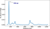 |
Fig. 1 2D dust extinction map illustrating the dust distribution as a function of distance up to 1.25 kpc from the Sun (Edenhofer et al. 2024). The peak at 154 pc indicates a distance corresponding to the Snake region. |
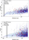 |
Fig. 2 Top panel: visual extinction (AV) as a function of the distance of stars within 2 kpc of the Sun. The extinction and distance values are derived from the StarHorse catalog. Lower panel: polarization percentage as a function of the distance. A vertical dashed line at 154 ± 15 pc marks the distance of the Snake filament. The error bars represent the uncertainties in the extinction and polarization measurements, scaled by 50%. The purple line represents the mean value in bins of 100 pc, with the light blue shaded area indicating the ±1σ uncertainty. |
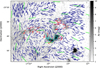 |
Fig. 3 Dust extinction map of the Snake region in color scale at a spatial resolution of 20″ from Román-Zúñiga et al. (2010). All segments represent the B-field orientation. Blue and red segments are inferred from the optical and NIR data, respectively, with S/N≥3. The green segments show the magnetic field orientation from Planck data at the resolution of 10′. The vectors are scaled to the same size to enhance visualization clarity. The cyan contours represent the C18O (1-0) integrated intensity at levels of 0.8 K km/s and 1.6 K km/s. |
3.2 Spatial distribution of the magnetic field
Figure 3 shows the dust extinction map of the Snake filament region at a spatial resolution of 20″ (Román-Zúñiga et al. 2010). Polarization vectors in optical, NIR, and submillimeter are plotted over the extinction map.
The submillimeter vectors are rotated by 90° to show the B-field orientation. The NIR data probe the denser part of the Snake filament, whereas the optical data trace the lower visual extinction of the observed field.
Figure 4 reveals two prominent peaks in the field lines orientation angles. These two peaks are visible in the optical, NIR, and submillimeter data. Specifically, the optical and NIR data exhibit their first peaks within the range of approximately 85° to 102. The optical data also show a second prominent peak at around 180°. In contrast, the submillimeter data reveal two distinct peaks at 66° and 169°, with the second peak of the NIR data aligning closely with the second peak observed in the submillimeter data.
In contrast, the infrared data have a random distribution in Fig. 4. The overall polarization distribution across the entire region does not appear to follow any specific pattern. However, it is important to note that the number of reliable NIR polarization detections is limited compared to the optical data, which reduces the statistical significance of any observed trends in the angle distribution. Despite this limitation, a peak in the distribution can be observed around 80° to 100°.
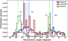 |
Fig. 4 Histogram of the distribution of magnetic polarization angles for the three datasets (optical, NIR, and submillimeter). Optical data peaks are highlighted by dashed blue lines and the submillimeter dataset distribution peaks by dashed green lines. |
3.3 The relative orientation of the filament with the magnetic field
To further characterize the Snake’s filamentary structure and its relationship with polarization data, we used the Python package radfill (Zucker & Chen 2018). The spine of the filament is defined by radfil using the fil_finder package (Koch & Rosolowsky 2015) based on the Av map and mask map provided. We extracted evenly spaced cuts perpendicular to the spine at intervals corresponding to every 7 pixels along its length. Consequently, the center of the resulting profiles aligns with the peak value of Av. Using this spine, we determined a filament length of 2.3 pc. Figure 5 illustrates the spine and the perpendicular cuts. We selected a 0.04 degree distance from the spine to make sure we covered the whole snake cloud in our sample (see Fig. 5). The plot also includes polarization data from optical and infrared wavelengths. The projections of the polarization vectors onto the spine was done by finding each polarization vector’s closest point on the spine and shifting it accordingly.
Our goal was to analyze how the polarization angles change as we move along the filament’s spine. The behavior of polarization vectors along the spine provides critical insights into the magnetic field geometry. Specifically, analyzing the relationship between the polarization vectors and the filament’s curvature allows us to evaluate whether the vectors are predominantly aligned with the filament (parallel) or if there are regions where they deviate significantly (perpendicular).
To quantify the alignment between the magnetic field vectors and the filament orientation, we calculated the projected Rayleigh statistic (PRS; Jow et al. 2018). This method provides a statistical measure of whether the polarization angles are preferentially aligned parallel or perpendicular to the filament’s local orientation (tangent to the spine). The filament spine is divided into 44 positions along its length. For each of these positions, we computed the PRS value using all polarization vectors projected onto that spine location (cyan vectors in Fig. 5), determined based on the closest spatial distance. Following Jow et al. (2018), the PRS was defined as
![Mathematical equation: $\[P R S=\frac{\sum_i^n ~\cos~ \theta_i}{\sqrt{n / 2}},\]$](/articles/aa/full_html/2025/08/aa54135-25/aa54135-25-eq5.png) (3)
(3)
where θ is twice the difference between the filament spine angle and the polarization angle. PRS >> 0 indicates strong parallel alignment, and PRS << 0 indicates strong perpendicular alignment. The uncertainty associated with the PRS value is from Jow et al. (2018):
![Mathematical equation: $\[\sigma^2=\frac{2 \sum_i^n\left(\cos~ \theta_i\right)^2-\mathrm{PRS}^2}{n}.\]$](/articles/aa/full_html/2025/08/aa54135-25/aa54135-25-eq6.png) (4)
(4)
Figure 6 shows the PRS values as a function of right ascension (RA), with error bars representing the uncertainties at each position along the spine. At both ends of the Snake filament, the polarization vectors are predominantly aligned with the spine, as indicated by PRS values greater than zero, above the dotted line. In contrast, near the central, denser region of the filament, the polarization vectors tend to become more perpendicular to the spine, reflected in the negative PRS values. The choice of maximum radius from the filament spine affects the PRS values, as it determines which polarization vectors are included in the analysis. To assess this effect, we performed the PRS calculation using a smaller radius of 0.02° (compared to a distance of 0.04° from the spine). The comparison reveals that approximately 9% of data show a change in the sign of their PRS value (from positive to negative or vice versa). This suggests that while the exact numerical values of PRS may vary slightly with radius, the overall conclusion regarding the alignment of the magnetic field with the filament spine remains robust within this tested range. We are committed to using a radius of 0.04° in our analysis, as this selection ensures that the entire Snake filament is encompassed, as defined by the boundaries of the dust extinction map.
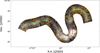 |
Fig. 5 Dust extinction map illustrating the masked filamentary structure. The spine of the filament is outlined by a prominent red curve, and the thin red lines indicate the locations of perpendicular cuts. Blue circles represent the peak pixel intensity along each cut. The orange vectors represent optical (S/N≥5) and infrared (S/N≥3) polarization segments. The cyan vectors are projections of all the orange polarization vectors onto the spine. Each polarization vector was projected by finding its closest point on the spine and shifting it accordingly. |
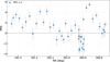 |
Fig. 6 PRS values as a function of RA. The PRS is calculated at each position along the filament spine using the group of polarization angles projected onto that location. Each point represents the PRS for a given spine position. The dotted line indicates PRS = 0, while the error bars represent the uncertainties. |
3.4 Spectral line fitting
CO isotopologues are widely utilized to probe gas in molecular clouds at varying densities. The 13CO (1-0) isotopologue is typically associated with tracing the diffuse outer regions of molecular clouds. In contrast, the rarer C18O (1-0) line, with a critical density of ~103 cm−3, serves as an excellent tracer for regions with higher column and volume densities (relative to 13CO (1-0)), effectively avoiding saturation. In this section we compare the polarization data with the gas kinematics using the complete set of NIR observations rather than limiting the analysis to data cross-matched with the StarHorse catalog (see Sect. 2.4). We established that no significant structures exist behind the Snake filament; therefore, all observed NIR data points are considered valid for this analysis.
Figure 7 displays the 13CO (1-0) and C18O (1-0) channel maps in 0.13 and 0.07 km s−1 steps, respectively. For both lines, the data presented have an S/N>3. Polarization vectors for optical (white) and NIR (cyan) wavelengths are overplotted on each panel. The 13CO (1-0) emission at velocities lower than 4.4 km s−1 is confined to the east region of the filament, while higher velocities show more concentrated emission at the center of the filamentary structure. At the filament’s center, velocities range from 4.53 km s−1 to 5.18 km s−1, transitioning from west to east (see the second row). While the C18O (1-0) emission is only concentrated at the center of the filament, it appears at lower velocities on the western side of the map and shifts to higher velocities toward the east side.
The kinematic properties of the observed C18O (1-0) molecular line were derived by fitting Gaussian profiles to each spectrum in the dataset using the Python package pyspeckit (Ginsburg & Mirocha 2011). A threshold of S/N > 5 was applied, ensuring the fits were constrained to regions with sufficient signal. A single-Gaussian fit was performed across the unmasked pixels with initial parameter guesses refined iteratively using neighboring pixel values. Fits with residuals exceeding twice the RMS or velocity dispersions (σv) broader than 0.35 km s−1 were masked and excluded. The resulting C18O (1-0) model cube showed only 0.1% of the pixels had a bad fit, demonstrating the robustness of the one-Gaussian fitting approach. The top panel of Fig. 8 displays the centroid velocity map of the C18O (1-0) line. The C18O (1-0) line exhibits a narrow linewidth, ranging from ~0.1 to 0.2 km s−1, indicative of quiescent C18O (1-0) gas dynamics in this region. Given that the sound speed in the region is cc = 0.2 km s−1 (for T = 15 K, from the Herschel map), these velocity dispersions suggest that the motions are transonic (see Appendix A for dispersion velocity map and sound speed calculation).
In contrast, the 13CO (1-0) line exhibits a more complex kinematics, particularly in the central regions of the Snake filament, where two velocity components are observed. Similar to C18O (1-0), a single-Gaussian fit was first applied to pixels with S/N > 4, followed by a dual-Gaussian fit for regions with significant residuals or broad line widths. Through visual inspection, we find that lines broader than 0.7 km s−1 exhibit profiles consistent with two velocity components. Based on this observation, we established a masking criterion that excludes pixels where the residuals exceed twice the RMS and velocity dispersions broader than 0.7 km s−1 in the single-Gaussian fit. Accurately fitting the 13CO (1-0) line with two Gaussian components in the central region of the Snake filament is challenging due to the line’s high opacity, which exceeds a value of 1 (see Sect. 3.5). The middle panel of Fig. 8 presents the centroid velocity map of the 13CO (1-0) line, derived using a single-Gaussian fitting. The central velocities (VLSR) of the 13CO (1-0) line range approximately from ~4.7km s−1 to ~5.2 km s−1, increasing from west to east.
A similar velocity gradient is observed in the C18O (1-0) line, with velocities increasing from lower to higher values from the west to the east side. The bottom panel of Fig. 8 presents six spectral profiles at different random positions along the Snake filament for both 13CO (1-0) and C18O (1-0) lines. These profiles highlight the saturation of the 13CO (1-0) line, which prevents an accurate Gaussian fit. For positions 1 to 3 (first row of the plot), the C18O (1-0) line shows no detectable signal, whereas the 13CO (1-0) line exhibits a strong signal with two distinct velocity components. In positions 4 to 6 (second row of the plot), both lines show clear signals, each with a single velocity component. The peak velocities of the 13CO (1-0) and C18O (1-0) lines are in good agreement.
Figure 9 presents a 3D position-position-velocity diagram of the C18O (1-0) line and the two velocity components of the 13CO (1-0) line. The higher velocity component of the 13CO (1-0) line overlaps significantly with the velocity of the C18O (1-0) line. From Figs. 8 and 9, we conclude that the two gas tracers follow the same cloud and with similar velocities. The gas shows lower velocities at both ends of the Snake filament, with velocities increasing toward the central region of the filamentary structure, which corresponds to the denser part of this region. This pattern suggests that gas is accreting toward the central region, a behavior also observed in other filaments (e.g., Feng et al. 2024). As discussed in Sect. 3.3, the magnetic field lines are aligned with the filament’s spine at both ends. We infer from this that the magnetic field plays a role in guiding material toward the central region of the filament, where the gas density increases. In this denser region, the magnetic field morphology becomes more complex, leading to the observed orientation of magnetic field lines that appear perpendicular to the filament’s spine.
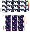 |
Fig. 7 (a) Channel maps between 4.01 and 5.44 km s−1 for the 13CO (1-0) spectral cube, in 0.13 km s−1 steps. White and cyan segments illustrate the B-field orientation in the optical (S/N≥5) and infrared (S/N≥3) bands, respectively. The velocity of each channel is shown on the top left of the panels. (b) Same as (a) but for the C18O (1-0) line. Channels are between 4.60 and 5.18 km s−1, in 0.07 km s−1 steps. |
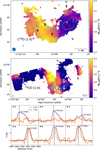 |
Fig. 8 Top panel: centroid velocity map of the C18O (1-0) line. Middle panel: Centroid velocity map of the 13CO (1-0) line. In both maps, we highlight six selected profiles at specific positions along the Snake, marked by white stars. The cyan contours represent the C18O (1-0) integrated intensity at levels of 0.8 K and 1.6 K. The beam size is shown in the bottom-left corner, and the scale bar in the bottom-right. Bottom panel: comparison of the six spectral profiles corresponding to the positions marked by white stars in both maps. The dashed orange profiles represent the C18O (1-0) line multiplied by 5, and the solid purple profiles correspond to the 13CO (1-0) line. The dashed black lines indicate the peak velocity of the 13CO (1-0) line, with the velocity values labeled next to them. |
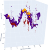 |
Fig. 9 Position-position-velocity plot illustrating the kinematics of the 13CO (1-0) and C18O (1-0) lines. Each data point represents the spatial location and centroid velocity of a Gaussian component, with colors distinguishing different Gaussian fits. The centroid velocity of the C18O (1-0) line is shown in orange, while the purple and red points correspond to the brighter and fainter intensity components of the 13CO (1-0) line, respectively. |
3.5 Line opacity
We estimated the opacity of 13CO (1-0) and C18O (1-0) using the following expression:
![Mathematical equation: $\[\tau=-~\ln~ \left[1-\frac{T_{\mathrm{mb}}}{J_\nu(T_{\mathrm{ex}})-J_\nu(T_{\mathrm{bg}})}\right],\]$](/articles/aa/full_html/2025/08/aa54135-25/aa54135-25-eq7.png) (5)
(5)
where Tex = 16 K is the excitation temperature derived from the Herschel dust temperature map, Tmb is the peak main beam temperature of the line, Jν represents the equivalent Rayleigh-Jeans temperature, and Tbg = 2.73 K is the temperature of the cosmic microwave background. To estimate uncertainties, we varied Tex within a physically meaningful range, ensuring that the lower limit does not exceed the minimum excitation temperature, Tex = 15 K. The optical depth of C18O (1-0) is determined to be ![Mathematical equation: $\[\tau=0.6_{-0.1}^{+0.1}\]$](/articles/aa/full_html/2025/08/aa54135-25/aa54135-25-eq8.png) , calculated using Tmb = 5.5 K. The uncertainties were estimated by considering a ±1 K variation in Tex. Similarly, for the 13CO (1-0) line, we obtain
, calculated using Tmb = 5.5 K. The uncertainties were estimated by considering a ±1 K variation in Tex. Similarly, for the 13CO (1-0) line, we obtain ![Mathematical equation: $\[\tau=2.1_{-0.9}^{+0.4}\]$](/articles/aa/full_html/2025/08/aa54135-25/aa54135-25-eq9.png) using Tmb = 11 K. These results confirm that the C18O (1-0) gas is optically thin, whereas the 13CO (1-0) gas is optically thick. The C18O (1-0) line has a relatively low critical density (nc ~ 103 cm−3), making it reasonable to consider that the excitation temperature (Tex) is approximately equal to the kinetic temperature (Tk), considering dust-gas coupling. Although the Herschel dust temperature is typically higher than the excitation temperature, as mentioned earlier, we also calculated the line opacity for a variation in Tex as an uncertainty.
using Tmb = 11 K. These results confirm that the C18O (1-0) gas is optically thin, whereas the 13CO (1-0) gas is optically thick. The C18O (1-0) line has a relatively low critical density (nc ~ 103 cm−3), making it reasonable to consider that the excitation temperature (Tex) is approximately equal to the kinetic temperature (Tk), considering dust-gas coupling. Although the Herschel dust temperature is typically higher than the excitation temperature, as mentioned earlier, we also calculated the line opacity for a variation in Tex as an uncertainty.
4 Discussion
4.1 Filament stability and absence of star formation
Filament stability can be assessed by comparing their mass-to-length ratio to a critical value (Ostriker 1964; Fiege & Pudritz 2000). To incorporate the effect of nonthermal motions, we followed the formulation introduced by Hacar et al. (2023):
![Mathematical equation: $\[\left(\frac{M}{L}\right)_{\mathrm{cr}}=m_{\mathrm{vir}}(\sigma_{\mathrm{tot}})=\frac{2 \sigma_{\mathrm{tot}}^2}{G} \sim 465\left(\frac{\sigma_{\mathrm{tot}}}{1 \mathrm{~km} \mathrm{~s}^{-1}}\right)^2 ~\mathrm{M}_{\odot} ~\mathrm{pc}^{-1},\]$](/articles/aa/full_html/2025/08/aa54135-25/aa54135-25-eq10.png) (6)
(6)
where G is the gravitational constant and M⊙ is the solar mass. σtot is the total gas velocity dispersion, ![Mathematical equation: $\[\sigma_{\text {tot }}^{2}=\sigma_{\text {nt }}^{2}+c_{\mathrm{s}}^{2}\]$](/articles/aa/full_html/2025/08/aa54135-25/aa54135-25-eq11.png) . For the detail calculation of the σtot, see Appendix A.
. For the detail calculation of the σtot, see Appendix A.
If the actual mass-to-length ratio of the filament, ![Mathematical equation: $\[\left(\frac{M}{L}\right)_{\text {fil }}\]$](/articles/aa/full_html/2025/08/aa54135-25/aa54135-25-eq12.png) , exceeds the critical value, the filament will collapse radially. To estimate the mass of the filament, we used the following equation:
, exceeds the critical value, the filament will collapse radially. To estimate the mass of the filament, we used the following equation:
![Mathematical equation: $\[M_{\mathrm{fil}}=1.13 \times 10^{-7} \times \sum_{i=1}^n\left(\frac{N\left(\mathrm{H}_2\right)}{\mathrm{cm}^{-2}}\right)_i\left(\frac{\theta}{\prime \prime}\right)^2\left(\frac{d_{\mathrm{cloud}}}{\mathrm{pc}}\right)^2 \mu_{\mathrm{H}_2} ~m_{\mathrm{H}} ~M_{\odot},\]$](/articles/aa/full_html/2025/08/aa54135-25/aa54135-25-eq13.png) (7)
(7)
where the summation ![Mathematical equation: $\[{\sum}_{i=1}^{n}\left(N\left(\mathrm{H}_{2}\right)_{i}\right)\]$](/articles/aa/full_html/2025/08/aa54135-25/aa54135-25-eq14.png) includes contributions from n pixels within the filament area as introduced in Sect. 3.3, mH = 1.67 × 10⁻²⁴ g is the mass of a hydrogen atom, μH2 = 2.8 (from Kauffmann et al. 2008) is the mean molecular weight per hydrogen molecule, and dcloud = 154 pc is the distance to the cloud, θ = 10″ is the pixel size. We calculated the gas column density of the filament, N(H2), from the visual extinction, AV (Fig. 3). Using the relation provided by Bohlin et al. (1978), N(H2) = 9.4 × 10²⁰ × AV cm−2 mag−1, we converted AV into the molecular hydrogen column density. The filament length is estimated to be L = 2.4 pc, with a detailed description of the measurement method provided in Sect. 3.3. The mass per unit length of the filament is determined to be 14.4 M⊙ pc−1, which is below the critical mass per unit length,
includes contributions from n pixels within the filament area as introduced in Sect. 3.3, mH = 1.67 × 10⁻²⁴ g is the mass of a hydrogen atom, μH2 = 2.8 (from Kauffmann et al. 2008) is the mean molecular weight per hydrogen molecule, and dcloud = 154 pc is the distance to the cloud, θ = 10″ is the pixel size. We calculated the gas column density of the filament, N(H2), from the visual extinction, AV (Fig. 3). Using the relation provided by Bohlin et al. (1978), N(H2) = 9.4 × 10²⁰ × AV cm−2 mag−1, we converted AV into the molecular hydrogen column density. The filament length is estimated to be L = 2.4 pc, with a detailed description of the measurement method provided in Sect. 3.3. The mass per unit length of the filament is determined to be 14.4 M⊙ pc−1, which is below the critical mass per unit length, ![Mathematical equation: $\[\left(\frac{M}{L}\right)_{\text {cr }}=31.3 ~M_{\odot} ~\mathrm{pc}^{-1}\]$](/articles/aa/full_html/2025/08/aa54135-25/aa54135-25-eq15.png) . This indicates that the Snake filament is stable against gravitational collapse. This finding is valid assuming negligible external pressure onto the filament. The magnetic field would only increase the support against collapse. Consequently, this is likely the primary reason for the absence of star formation in this region.
. This indicates that the Snake filament is stable against gravitational collapse. This finding is valid assuming negligible external pressure onto the filament. The magnetic field would only increase the support against collapse. Consequently, this is likely the primary reason for the absence of star formation in this region.
We checked for the presence of recent star formation activity using version 7.1 of the SPHEREx Target List of ICE Sources (SPLICES), which is part of the SPHEREx all-sky survey mission (Ashby et al. 2023). The catalog contains 8.6 × 10⁶ objects that are brighter than approximately 12 Vega magnitudes in the W2 band. To identify young stellar objects (YSOs), we used the W1[3.6 mag]–W2[4.5 mag] versus W2[4.5 mag]–W3[5.8 mag] color-color diagram of asymptotic giant branch candidates from SPLICES (see Ashby et al. 2023). The regions defined by Koenig & Leisawitz (2014) for the selection of Class I and Class II YSOs. No YSOs have been detected in the area using the Spitzer GLIMPSE color-color diagram. We utilized the mid-infrared colors [3.6–4.5] versus [4.5–5.8] to identify YSOs in the region. We considered a region of size 2 pc that encompasses the filamentary features associated with the Snake region, shown in Fig. 3, and find 822 objects that are detected in the region (black dots in Fig. 10). We applied a distance constraint, selecting objects that are 1 kpc away, and we only find 19 objects within 1 kpc. Among these, we identify only one object as Class II, which is situated far from the Snake region.
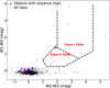 |
Fig. 10 W1–W2 versus W2–W3 color–color diagram of asymptotic giant branch candidates from the SPLICES survey. The areas within the dashed lines are those used by Koenig & Leisawitz (2014) to identify Class I and Class II YSOs. Black dots represent all the data from SPLICES, and purple diamonds indicate objects within a distance of 1 kpc. |
4.2 Polarization efficiency
Figure 11 presents the scatter plots of polarization efficiency (ppol/AV) as a function of visual extinction (AV) in log-log space. The optical and NIR datasets are organized into 30 bins. The error bars on each data point are calculated as the standard deviation of the polarization measurements within each bin, reflecting the measurement uncertainties in the analysis. The optical and NIR data show a peak density within the visual extinction range of 1–3 magnitudes.
The plot includes two fitted lines corresponding to two datasets. The optical fit is represented by the equation: ppol/AV = −(0.73 ± 0.09) log AV + 0.04. Conversely, the NIR fit is described by ppol/AV = −(0.75 ± 0.27) log AV + 0.02, which shows a slightly steeper decline in polarization efficiency with increasing visual extinction; however, the two follow the same overall trend, as they span very similar ranges of extinction values. The optical polarization is primarily associated with the diffuse cloud surrounding the Snake filament, while the infrared data predominantly trace slightly denser regions. However, both datasets in our analysis correspond to relatively low-density regions within the Snake filament, spanning a visual extinction range of 0.5 to 4.5 magnitudes (see Fig. 3). The polarization efficiency exhibits a decrease at both optical and infrared wavelengths. The slopes observed for both datasets indicate depolarization in this region, consistent with the radiative alignment theory (Lazarian & Hoang 2007). As visual extinction increases, reduced radiation penetration within the cloud diminishes the effectiveness of radiative torques in aligning dust grains. As reported by Alves et al. (2014), NIR polarization measurements of the starless core Pipe-109 in the Pipe Nebula yield α (which is the slope of the fit) values of 1.0 for AV < 9.5 mag and 0.34 for AV > 9.5 mag. Redaelli et al. (2019) determined a steep slope of α = 1.21 for the FIR polarization data associated with the protostellar core IRAS 15398-3359. Similarly, Tabatabaei et al. (2024) derived a slope of 0.75 from NIR data of a filamentary structure in Barnard 59. However, other mechanisms may also contribute to this depolarization trend. Seifried et al. (2019) conducted radiative transfer modeling using the POLARIS code and show that dust grains remain well aligned even at high densities (n > 103 cm−3) and extinctions (AV > 1), provided the radiative alignment theory alignment is active. They found that the frequently observed decrease in polarization degree is primarily caused by large variations in the magnetic field orientation along the line of sight, rather than a breakdown of grain alignment. Wang et al. (2019) reported a power-law slope of α = 0.56 from 850 μm polarization observations of the IC 5146 filament, which implies that dust grains in this AV ~ 20–300 mag range can still be aligned with magnetic fields.
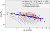 |
Fig. 11 Scatter plots of the polarization efficiency (ppol/AV) as a function of the visual extinction (AV) in magnitudes in logarithmic scale. Measurement uncertainties are displayed as an error bar for each data point. Solid lines are the best fit for the datasets, as explained in the main text. Contours represent levels of constant probability density estimated using a 2D kernel density estimation of the data (using the seaborn Python library; Waskom 2021). These contours indicate where the data points are most densely concentrated. Both sets of contours span density levels from 0 to 0.8, with steps of 0.1, effectively highlighting regions of high and low data concentration. The best-fit parameters are shown in the top-right corner. |
5 Summary
In this work, we investigated the magnetic field geometry and kinematic properties of the Snake filament by combining archival submillimeter polarimetry from Planck and molecular line data from IRAM with new optical and NIR polarization measurements. Our analysis confirms that the Snake is the dominant dust structure along the line of sight within 2 kpc of the Sun, with no significant molecular structures located beyond this distance. As a result, the observed polarization angles of background stars trace the magnetic field associated with the Snake filament. Additionally, we determined the distance of the source to be 154 pc using Gaia data (see Sect. 3.1). This distance puts the Snake filament at the same distance as the Pipe Nebula.
The Snake filament is gravitationally stable. The estimated mass-to-length ratio is below the critical threshold, explaining the lack of star formation in the region. The polarization efficiency (ppol/AV) decreases with increasing visual extinction, with fitted slopes of 0.73 for optical data and 0.75 for NIR data. This behavior suggests depolarization in denser regions, where reduced radiation penetration weakens the dust–grain alignment.
Kinematic analysis reveals a velocity gradient along the filament in both 13CO (1-0) and C18O (1-0) data. The C18O (1-0) line, tracing denser regions, exhibits well-constrained single-Gaussian fits, while the 13CO (1-0) line shows more complex kinematics, including multiple velocity components in the denser central region. Furthermore, the polarization vectors along the filament’s spine exhibit a strong alignment with the filament’s spine tangent at both ends. Consequently, it appears that the field may help channel material toward the central region, where the gas density increases. In this denser central area, the magnetic field morphology appears more complex, resulting in field lines that are oriented perpendicular to the filament’s spine.
These results demonstrate that the Snake filament is immersed in a well-ordered magnetic field, which plays a critical role in maintaining its structural coherence and stability. The observed polarization and kinematics suggest that magnetic fields significantly influence the dynamics of the filament, shaping its evolution. This study contributes to our understanding of the role of magnetic fields in filamentary structures and their connection to star formation processes.
Acknowledgements
Elena Redaelli acknowledges the support from the Minerva Fast Track Program of the Max Planck Society. G. Franco acknowledges the partial support from the Brazilian agencies CNPq and FAPEMIG. We thank the staff of OPD/LNA (Brazil) for their hospitality and invaluable help during our observing runs. This research has used data from the Herschel Gould Belt survey (HGBS) project (http://gouldbelt-herschel.cea.fr). The HGBS is a Herschel Key Programme jointly carried out by SPIRE Specialist Astronomy Group 3 (SAG 3), scientists of several institutes in the PACS Consortium (CEA Saclay, INAF-IFSI Rome, and INAF-Arcetri, KU Leuven, MPIA Heidelberg), and scientists of the Herschel Science Center (HSC). This work has made use of data from the European Space Agency (ESA) mission Gaia (https://www.cosmos.esa.int/gaia), processed by the Gaia Data Processing and Analysis Consortium (DPAC, https://www.cosmos.esa.int/web/gaia/dpac/consortium). Funding for the DPAC has been provided by national institutions, in particular the institutions participating in the Gaia Multilateral Agreement. The authors express their gratitude to Jaime Pineda for his valuable support with the data reduction process of the IRAM data.
Appendix A Velocity dispersions
The linewidth of the observed C18O (1-0) molecular line was determined by fitting Gaussian profiles to each spectrum in the data cube. Figure A.1 illustrates the derived velocity dispersion map, σv, highlighting the narrow linewidths of the C18O (1-0) emission, with values typically around 0.1 km s−1 to 0.2 km s−1. The isothermal sound speed was obtained from
![Mathematical equation: $\[c_{\mathrm{s}}=\sqrt{\frac{k_{\mathrm{B}} T}{\mu m_{\mathrm{H}}}}=0.2 ~\mathrm{kms}^{-1},\]$](/articles/aa/full_html/2025/08/aa54135-25/aa54135-25-eq16.png) (A.1)
(A.1)
where μ = 2.37 (Kauffmann et al. 2008) is the mean molecular weight per free particle and mH is the mass of hydrogen atom. We used the dust temperature, Td = 15 K from Herschel map as a proxy for the gas kinetic temperature.
The nonthermal velocity dispersion of the gas can be derived from
![Mathematical equation: $\[\sigma_{\mathrm{nt}}=\sqrt{\sigma_{\mathrm{v}}^2-\sigma_{\mathrm{th}}^2}=0.14 ~\mathrm{kms}^{-1},\]$](/articles/aa/full_html/2025/08/aa54135-25/aa54135-25-eq17.png) (A.2)
(A.2)
with ![Mathematical equation: $\[\sigma_{\text {th }}=\sqrt{k_{\mathrm{B}} T / m_{\text {obs }}}=0.06\]$](/articles/aa/full_html/2025/08/aa54135-25/aa54135-25-eq18.png) km s−1 and σv = 0.15 km s−1, where mobs is the mass of observed molecule line, C18O (1-0). As mentioned in the main text, the total gas velocity dispersion is calculated using
km s−1 and σv = 0.15 km s−1, where mobs is the mass of observed molecule line, C18O (1-0). As mentioned in the main text, the total gas velocity dispersion is calculated using
![Mathematical equation: $\[\sigma_{\mathrm{tot}}=\sqrt{\sigma_{\mathrm{nt}}^2+c_{\mathrm{s}}^2}=0.24 ~\mathrm{kms}^{-1}.\]$](/articles/aa/full_html/2025/08/aa54135-25/aa54135-25-eq19.png) (A.3)
(A.3)
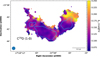 |
Fig. A.1 Velocity dispersion (σV) map of the C18O (1-0) line. The cyan contours represent the C18O (1-0) integrated intensity at levels 0.8 and 1.6 K. The beam size is indicated in the bottom-left corner, and the scale bar in the bottom-right. |
References
- Alves, F. O., & Franco, G. A. P. 2007, A&A, 470, 597 [NASA ADS] [CrossRef] [EDP Sciences] [Google Scholar]
- Alves, F. O., Frau, P., Girart, J. M., et al. 2014, A&A, 569, L1 [NASA ADS] [CrossRef] [EDP Sciences] [Google Scholar]
- Anders, F., Khalatyan, A., Queiroz, A. B. A., et al. 2022, A&A, 658, A91 [NASA ADS] [CrossRef] [EDP Sciences] [Google Scholar]
- André, P., Men’shchikov, A., Bontemps, S., et al. 2010, A&A, 518, L102 [NASA ADS] [CrossRef] [EDP Sciences] [Google Scholar]
- André, P., Di Francesco, J., Ward-Thompson, D., et al. 2014, in Protostars and Planets VI, eds. H. Beuther, R. S. Klessen, C. P. Dullemond, & T. Henning, 27 [Google Scholar]
- Ashby, M. L. N., Hora, J. L., Lakshmipathaiah, K., et al. 2023, ApJ, 949, 105 [Google Scholar]
- Bohlin, R. C., Savage, B. D., & Drake, J. F. 1978, ApJ, 224, 132 [Google Scholar]
- Carrasco, J. M., Weiler, M., Jordi, C., et al. 2021, A&A, 652, A86 [NASA ADS] [CrossRef] [EDP Sciences] [Google Scholar]
- Chambers, K. C., Magnier, E. A., Metcalfe, N., et al. 2016, arXiv e-prints [arXiv:1612.05560] [Google Scholar]
- Corradi, R. L. M., Aznar, R., & Mampaso, A. 1998, MNRAS, 297, 617 [CrossRef] [Google Scholar]
- Crutcher, R. M. 2012, ARA&A, 50, 29 [Google Scholar]
- Cutri, R. M., Skrutskie, M. F., van Dyk, S., et al. 2003, 2MASS All Sky Catalog of point sources [Google Scholar]
- Cutri, R. M., Wright, E. L., Conrow, T., et al. 2013, Explanatory Supplement to the AllWISE Data Release Products [Google Scholar]
- Dzib, S. A., Loinard, L., Ortiz-León, G. N., Rodríguez, L. F., & Galli, P. A. B. 2018, ApJ, 867, 151 [Google Scholar]
- Edenhofer, G., Zucker, C., Frank, P., et al. 2024, A&A, 685, A82 [NASA ADS] [CrossRef] [EDP Sciences] [Google Scholar]
- Feng, J., Smith, R. J., Hacar, A., Clark, S. E., & Seifried, D. 2024, MNRAS, 528, 6370 [NASA ADS] [CrossRef] [Google Scholar]
- Fiege, J. D., & Pudritz, R. E. 2000, MNRAS, 311, 85 [Google Scholar]
- Gaia Collaboration (Prusti, T., et al.) 2016, A&A, 595, A1 [NASA ADS] [CrossRef] [EDP Sciences] [Google Scholar]
- Gaia Collaboration (Brown, A. G. A., et al.) 2021, A&A, 649, A1 [NASA ADS] [CrossRef] [EDP Sciences] [Google Scholar]
- Gaia Collaboration (Vallenari, A., et al.) 2023, A&A, 674, A1 [NASA ADS] [CrossRef] [EDP Sciences] [Google Scholar]
- Ginsburg, A., & Mirocha, J. 2011, PySpecKit: Python Spectroscopic Toolkit, Astrophysics Source Code Library [record ascl:1109.001] [Google Scholar]
- Hacar, A., Clark, S. E., Heitsch, F., et al. 2023, in Astronomical Society of the Pacific Conference Series, 534, Protostars and Planets VII, eds. S. Inutsuka, Y. Aikawa, T. Muto, K. Tomida, & M. Tamura, 153 [Google Scholar]
- Hennebelle, P., & Inutsuka, S.-i. 2019, Front. Astron. Space Sci., 6, 5 [Google Scholar]
- Jow, D. L., Hill, R., Scott, D., et al. 2018, MNRAS, 474, 1018 [NASA ADS] [CrossRef] [Google Scholar]
- Kauffmann, J., Bertoldi, F., Bourke, T. L., Evans, N. J., I., & Lee, C. W. 2008, A&A, 487, 993 [NASA ADS] [CrossRef] [EDP Sciences] [Google Scholar]
- Koch, E. W., & Rosolowsky, E. W. 2015, MNRAS, 452, 3435 [Google Scholar]
- Koenig, X. P., & Leisawitz, D. T. 2014, ApJ, 791, 131 [Google Scholar]
- Könyves, V., André, P., Men’shchikov, A., et al. 2015, A&A, 584, A91 [Google Scholar]
- Lazarian, A., & Hoang, T. 2007, MNRAS, 378, 910 [Google Scholar]
- Li, H. B., Goodman, A., Sridharan, T. K., et al. 2014, in Protostars and Planets VI, eds. H. Beuther, R. S. Klessen, C. P. Dullemond, & T. Henning, 101 [Google Scholar]
- Magalhaes, A. M., Rodrigues, C. V., Margoniner, V. E., Pereyra, A., & Heathcote, S. 1996, in Astronomical Society of the Pacific Conference Series, 97, Polarimetry of the Interstellar Medium, eds. W. G. Roberge & D. C. B. Whittet, 118 [Google Scholar]
- Nielbock, M., Launhardt, R., Steinacker, J., et al. 2012, A&A, 547, A11 [NASA ADS] [CrossRef] [EDP Sciences] [Google Scholar]
- Onken, C. A., Wolf, C., Bessell, M. S., et al. 2019, PASA, 36, e033 [Google Scholar]
- Ostriker, J. 1964, ApJ, 140, 1056 [Google Scholar]
- Pattle, K., Fissel, L., Tahani, M., Liu, T., & Ntormousi, E. 2023, in Astronomical Society of the Pacific Conference Series, 534, Protostars and Planets VII, eds. S. Inutsuka, Y. Aikawa, T. Muto, K. Tomida, & M. Tamura, 193 [Google Scholar]
- Pillai, T. G. S., Clemens, D. P., Reissl, S., et al. 2020, Nat. Astron., 4, 1195 [Google Scholar]
- Planck Collaboration Int. XXXV. 2016, A&A, 586, A138 [NASA ADS] [CrossRef] [EDP Sciences] [Google Scholar]
- Ramírez, E. A., Magalhães, A. M., Davidson, Jr., J. W., Pereyra, A., & Rubinho, M. 2017, PASP, 129, 055001 [Google Scholar]
- Redaelli, E., Alves, F. O., Santos, F. P., & Caselli, P. 2019, A&A, 631, A154 [NASA ADS] [CrossRef] [EDP Sciences] [Google Scholar]
- Román-Zúñiga, C. G., Alves, J. F., Lada, C. J., & Lombardi, M. 2010, ApJ, 725, 2232 [Google Scholar]
- Roy, A., André, P., Palmeirim, P., et al. 2014, A&A, 562, A138 [NASA ADS] [CrossRef] [EDP Sciences] [Google Scholar]
- Seifried, D., Walch, S., Reissl, S., & Ibáñez-Mejía, J. C. 2019, MNRAS, 482, 2697 [NASA ADS] [CrossRef] [Google Scholar]
- Soler, J. D., Ade, P. A. R., Angilè, F. E., et al. 2017, A&A, 603, A64 [CrossRef] [EDP Sciences] [Google Scholar]
- Tabatabaei, F. S., Redaelli, E., Galli, D., et al. 2024, A&A, 688, A98 [NASA ADS] [CrossRef] [EDP Sciences] [Google Scholar]
- Vergely, J. L., Lallement, R., & Cox, N. L. J. 2022, A&A, 664, A174 [NASA ADS] [CrossRef] [EDP Sciences] [Google Scholar]
- Wang, J.-W., Lai, S.-P., Eswaraiah, C., et al. 2019, ApJ, 876, 42 [Google Scholar]
- Ward-Thompson, D., André, P., Crutcher, R., et al. 2007, in Protostars and Planets V, eds. B. Reipurth, D. Jewitt, & K. Keil, 33 [Google Scholar]
- Waskom, M. L. 2021, J. Open Source Softw., 6, 3021 [CrossRef] [Google Scholar]
- Zhang, X., Green, G. M., & Rix, H.-W. 2023, MNRAS, 524, 1855 [NASA ADS] [CrossRef] [Google Scholar]
- Zucker, C., & Chen, H. H.-H. 2018, ApJ, 864, 152 [NASA ADS] [CrossRef] [Google Scholar]
The OPD is operated by the Brazilian LNA, a research institute of the Ministry of Science, Technology and Innovation (MCTI).
We downloaded the data from https://pla.esac.esa.int/, which uses the IAU convention. If the data are downloaded from https://irsa.ipac.caltech.edu/applications/planck/, the derived polarization position angle should be ϕ = 0.5 tan−1(−U/Q).
All Figures
|
Fig. 1 2D dust extinction map illustrating the dust distribution as a function of distance up to 1.25 kpc from the Sun (Edenhofer et al. 2024). The peak at 154 pc indicates a distance corresponding to the Snake region. |
| In the text | |
|
Fig. 2 Top panel: visual extinction (AV) as a function of the distance of stars within 2 kpc of the Sun. The extinction and distance values are derived from the StarHorse catalog. Lower panel: polarization percentage as a function of the distance. A vertical dashed line at 154 ± 15 pc marks the distance of the Snake filament. The error bars represent the uncertainties in the extinction and polarization measurements, scaled by 50%. The purple line represents the mean value in bins of 100 pc, with the light blue shaded area indicating the ±1σ uncertainty. |
| In the text | |
|
Fig. 3 Dust extinction map of the Snake region in color scale at a spatial resolution of 20″ from Román-Zúñiga et al. (2010). All segments represent the B-field orientation. Blue and red segments are inferred from the optical and NIR data, respectively, with S/N≥3. The green segments show the magnetic field orientation from Planck data at the resolution of 10′. The vectors are scaled to the same size to enhance visualization clarity. The cyan contours represent the C18O (1-0) integrated intensity at levels of 0.8 K km/s and 1.6 K km/s. |
| In the text | |
|
Fig. 4 Histogram of the distribution of magnetic polarization angles for the three datasets (optical, NIR, and submillimeter). Optical data peaks are highlighted by dashed blue lines and the submillimeter dataset distribution peaks by dashed green lines. |
| In the text | |
|
Fig. 5 Dust extinction map illustrating the masked filamentary structure. The spine of the filament is outlined by a prominent red curve, and the thin red lines indicate the locations of perpendicular cuts. Blue circles represent the peak pixel intensity along each cut. The orange vectors represent optical (S/N≥5) and infrared (S/N≥3) polarization segments. The cyan vectors are projections of all the orange polarization vectors onto the spine. Each polarization vector was projected by finding its closest point on the spine and shifting it accordingly. |
| In the text | |
|
Fig. 6 PRS values as a function of RA. The PRS is calculated at each position along the filament spine using the group of polarization angles projected onto that location. Each point represents the PRS for a given spine position. The dotted line indicates PRS = 0, while the error bars represent the uncertainties. |
| In the text | |
|
Fig. 7 (a) Channel maps between 4.01 and 5.44 km s−1 for the 13CO (1-0) spectral cube, in 0.13 km s−1 steps. White and cyan segments illustrate the B-field orientation in the optical (S/N≥5) and infrared (S/N≥3) bands, respectively. The velocity of each channel is shown on the top left of the panels. (b) Same as (a) but for the C18O (1-0) line. Channels are between 4.60 and 5.18 km s−1, in 0.07 km s−1 steps. |
| In the text | |
|
Fig. 8 Top panel: centroid velocity map of the C18O (1-0) line. Middle panel: Centroid velocity map of the 13CO (1-0) line. In both maps, we highlight six selected profiles at specific positions along the Snake, marked by white stars. The cyan contours represent the C18O (1-0) integrated intensity at levels of 0.8 K and 1.6 K. The beam size is shown in the bottom-left corner, and the scale bar in the bottom-right. Bottom panel: comparison of the six spectral profiles corresponding to the positions marked by white stars in both maps. The dashed orange profiles represent the C18O (1-0) line multiplied by 5, and the solid purple profiles correspond to the 13CO (1-0) line. The dashed black lines indicate the peak velocity of the 13CO (1-0) line, with the velocity values labeled next to them. |
| In the text | |
|
Fig. 9 Position-position-velocity plot illustrating the kinematics of the 13CO (1-0) and C18O (1-0) lines. Each data point represents the spatial location and centroid velocity of a Gaussian component, with colors distinguishing different Gaussian fits. The centroid velocity of the C18O (1-0) line is shown in orange, while the purple and red points correspond to the brighter and fainter intensity components of the 13CO (1-0) line, respectively. |
| In the text | |
|
Fig. 10 W1–W2 versus W2–W3 color–color diagram of asymptotic giant branch candidates from the SPLICES survey. The areas within the dashed lines are those used by Koenig & Leisawitz (2014) to identify Class I and Class II YSOs. Black dots represent all the data from SPLICES, and purple diamonds indicate objects within a distance of 1 kpc. |
| In the text | |
|
Fig. 11 Scatter plots of the polarization efficiency (ppol/AV) as a function of the visual extinction (AV) in magnitudes in logarithmic scale. Measurement uncertainties are displayed as an error bar for each data point. Solid lines are the best fit for the datasets, as explained in the main text. Contours represent levels of constant probability density estimated using a 2D kernel density estimation of the data (using the seaborn Python library; Waskom 2021). These contours indicate where the data points are most densely concentrated. Both sets of contours span density levels from 0 to 0.8, with steps of 0.1, effectively highlighting regions of high and low data concentration. The best-fit parameters are shown in the top-right corner. |
| In the text | |
|
Fig. A.1 Velocity dispersion (σV) map of the C18O (1-0) line. The cyan contours represent the C18O (1-0) integrated intensity at levels 0.8 and 1.6 K. The beam size is indicated in the bottom-left corner, and the scale bar in the bottom-right. |
| In the text | |
Current usage metrics show cumulative count of Article Views (full-text article views including HTML views, PDF and ePub downloads, according to the available data) and Abstracts Views on Vision4Press platform.
Data correspond to usage on the plateform after 2015. The current usage metrics is available 48-96 hours after online publication and is updated daily on week days.
Initial download of the metrics may take a while.