| Issue |
A&A
Volume 700, August 2025
|
|
|---|---|---|
| Article Number | A225 | |
| Number of page(s) | 23 | |
| Section | Planets, planetary systems, and small bodies | |
| DOI | https://doi.org/10.1051/0004-6361/202554431 | |
| Published online | 20 August 2025 | |
Interaction of Trappist-1 exoplanets with coronal mass ejections: Joule heating, Poynting fluxes, and the role of magnetic fields
1
Institute for Geophysics and Meteorology, University of Cologne,
Pohligstr. 3,
50969
Cologne,
Germany
2
Leiden Observatory, Leiden University,
Einsteinweg 55,
2333 CC
Leiden,
The Netherlands
★ Corresponding authors: This email address is being protected from spambots. You need JavaScript enabled to view it.
; This email address is being protected from spambots. You need JavaScript enabled to view it.
Received:
8
March
2025
Accepted:
17
June
2025
Abstract
Context. Flares and associated coronal mass ejections (CMEs) are energetic stellar phenomena that drastically shape the space weather around planets. Close-in exoplanets orbiting active cool stars are likely exposed to particularly extreme space weather, and the effects on the planets are not understood well enough. The terrestrial Trappist-1 exoplanets are excellent subjects to study the impact of CMEs on close-in planetary bodies, their atmospheres and ultimately their habitability.
Aims. Our aim is to better understand the role of planetary magnetic fields in shielding the planet energetically from external forcing. We expand on recent studies of CME-induced Joule heating of planetary interiors and atmospheres by including a magnetohydrodynamic (MHD) model of the interaction.
Methods. We studied the interaction of CMEs with Trappist-1b and e using time-dependent MHD simulations. We considered magnetic flux rope and non-magnetized DP CMEs. We calculated induction heating in the planetary interior and ionospheric Joule heating for various intrinsic magnetic field strengths and CME energies.
Results. Magnetospheric compression is the main driver of magnetic variability. Planetary magnetic fields enhance induction heating in the interior, although the effect is weaker with flux rope CMEs. Single event dissipation rates with 1-hour CMEs amount to 20 TW and 1 TW for Trappist-1b and e, respectively. Taking into account CME occurrence rates, the annual average heating rates are ≈10 TW (b) and 1 TW (e), which are placed near the lower end of previously estimated dissipation rates. Within the range of the studied planetary magnetic field strengths, Bp, magnetospheric inward Poynting fluxes scale with B3p. Thus, stronger magnetic fields increase the absorption of CME energy. Ionospheric Joule heating rates amount to 103-4 TW and decrease for stronger magnetic fields, Bp. These heating rates exceed the average stellar XUV input by one to two orders of magnitude and might severely impact atmospheric erosion. In a steady state, stellar wind ionospheric Joule heating amounts to ≈102 TW.
Key words: magnetohydrodynamics (MHD) / planets and satellites: atmospheres / planets and satellites: magnetic fields / planets and satellites: terrestrial planets / planet–star interactions / planets and satellites: individual: Trappist-1
© The Authors 2025
 Open Access article, published by EDP Sciences, under the terms of the Creative Commons Attribution License (https://creativecommons.org/licenses/by/4.0), which permits unrestricted use, distribution, and reproduction in any medium, provided the original work is properly cited.
This article is published in open access under the Subscribe to Open model. This email address is being protected from spambots. You need JavaScript enabled to view it. to support open access publication.
1 Introduction
In the Solar System, flares and associated coronal mass ejections (CMEs) are the most energetic solar events, and they drastically affect the space weather around the planets. Flares and CMEs both originate from the energy release caused by a magnetic reconnection in the stellar atmosphere (Compagnino et al. 2017; Chen 2011; Shibata & Magara 2011; Chen et al. 2006), and thus, CME mass and velocity are generally correlated with the flare energy. So far there have been no fully conclusive observations of extrasolar CMEs, but it can be assumed that such eruptive events are particularly common around cool stars and are much more extreme than the case in the Solar System (Moschou et al. 2019).
Low mass M-dwarfs are magnetically very active and show strong flaring activity with high X-ray luminosities exceeding Solar extreme events (Paudel et al. 2018; Moschou et al. 2019; Seli et al. 2021; Yang et al. 2023). From observations of the Sun, it is known that high flare X-ray energies typically correspond to strong CMEs (Youssef 2012; Moschou et al. 2019). M-dwarfs are the most common stars in the Universe, and many exoplanets have been found in the systems they comprise. This raises the question of what space weather is like in such systems and how it affects the planet’s space environment, atmosphere, and interior. Another important factor is the role of planetary magnetic fields in shielding the planets and their atmospheres from space weather and whether intrinsic magnetic fields support or hinder habitability (Airapetian et al. 2018; Tilley et al. 2019; Airapetian et al. 2020). We address the question about the role of intrinsic magnetic fields in regard to electromagnetic shielding by investigating how they influence the absorption and dissipation of energy in the space environment and interior.
A promising target for studies investigating environmental effects on exoplanets is the Trappist-1 system, which hosts seven terrestrial exoplanets. Trappist-1 is a flaring star (Vida et al. 2017; Paudel et al. 2018; Glazier et al. 2020; Howard et al. 2023) with three planets residing in the habitable zone (Gillon et al. 2017; Payne & Kaltenegger 2024).
Trappist-1b has no atmosphere (Greene et al. 2023), and there are indications of at most a thin atmosphere around Trappist-1c (Zieba et al. 2023; Lincowski et al. 2023). The existence of atmospheres on the other planets has not been conclusively clarified, and several modeling studies have made different predictions on the existence of atmospheres, atmospheric retention, and secondary atmosphere production (e.g., Van Looveren et al. 2024; Krissansen-Totton et al. 2024; Krissansen-Totton 2023; Krishnamurthy et al. 2021; Dong et al. 2018; de Wit et al. 2018; Bourrier et al. 2017). The models used by these studies rely heavily on our knowledge of planetary energy budgets, and therefore a detailed understanding of possible energy sources for the planetary system is crucial. Especially for cool exoplanet host stars in their pre-main sequence phase, stellar wind energy input may provide an important energy supply in addition to high stellar irradiation. Strong interior heat sources may drive geodynamic processes that have been shown to play a key role for habitability by supporting the carbon cycle caused by tectonic subduction (Airapetian et al. 2020; Höning & Spohn 2023), by determining the equilibrium state land-ocean fraction (Höning et al. 2019), or by affecting secondary atmosphere compositions through outgassing and volcanism (Tosi et al. 2017; Godolt et al. 2019; Airapetian et al. 2020; Unterborn et al. 2022). In general, star-planet interactions provide many mechanisms for energy exchange between stars, stellar winds, and planets. Tidal interactions, for example, can contribute significantly to the interior energy budget (e.g., for Io; Peale et al. 1979; Tyler et al. 2015; Davies et al. 2024). Modeling studies have suggested that Trappist-1 planets might be subject to a strong tidal heating, with Trappist-1b exhibiting a heat production rate similar to Io (≈100 TW and up to 1000 TW in extreme scenarios). Trappist-1c – e may experience a tidally induced heat production rate similar to that of the Earth (Luger et al. 2017; Barr et al. 2018; Dobos et al. 2019) (a few terawatts). Bolmont et al. (2020) calculated the tidal dissipation of Trappist-1e as being on the order of 1-10 TW for a multi-layered planet and several hundred terawatts for a homogeneous planet. High-energy radiation from exoplanet host stars significantly influences the temperature on planetary surfaces and photochemical processes in the atmospheres, if present (Tilley et al. 2019; García Muñoz 2023), or facilitates atmospheric escape (Roettenbacher & Kane 2017; Airapetian et al. 2017; Bourrier et al. 2017). It has also been suggested that the planet’s motion through a variable stellar magnetic field may impact the interior of exoplanets by Ohmic dissipation (Kislyakova & Noack 2020). Varying stellar winds and magnetic fields may also lead to significant Ohmic dissipation (i.e., Joule heating) within the upper atmospheres (Strugarek et al. 2025), which has also been shown for Trappist-1e (Cohen et al. 2024).
In this paper, we address the question of whether space weather, more precisely magnetic variability imposed by planetintersecting CMEs, dissipate energy within close-in rocky exoplanets and their atmospheres. We study the energy dissipation as a function of the associated flare energy and planetary magnetic field strength. We address how the planets’ magnetic fields influence the intake of CME energy into the magnetosphere and whether magnetic fields in general shield the planet energetically from its space environment.
Interior heating of terrestrial planets due to electromagnetic induction has been investigated in previous studies. A planet’s motion through a time variable stellar magnetic field has been considered (Kislyakova et al. 2017, 2018; Kislyakova & Noack 2020). However, these studies assumed favorably inclined stellar magnetic fields and outdated stellar rotation rates that were too fast (e.g., Trappist-1; Kislyakova et al. 2017). These studies suggest a high probability of molten or partially molten exoplanets or local magma oceans, which might cause a volcanically driven atmosphere. However, recent observations have shown that Trappist-1b may have no atmosphere (e.g., Greene et al. 2023). A more recent study used a Trappist-1 flare frequency distribution to estimate the occurrence rate of CMEs intersecting the planets (Grayver et al. 2022). The geomagnetic response of the terrestrial magnetic field environment was scaled to CME events associated with flare energies from the observed flare frequency distribution (Paudel et al. 2018). The study showed that CME-induced Ohmic dissipation in planetary interiors represents a permanent heating mechanism that influences interior heat budgets. Grayver et al. (2022) considered Earth-like magnetized and non-magnetized planets and found that planetary magnetic fields amplify the interior heating significantly.
In this work, we aim to extend the modeling of CME-induced interior heating of Grayver et al. (2022) by considering the full plasma interaction between interplanetary CMEs and planets, taking into account a parameter range to describe intrinsic magnetic fields, and better understand the role of planetary magnetic fields in such star-planet magnetic interactions. We consider flare frequency distributions for Trappist-1 obtained from dedicated observing campaigns (Paudel et al. 2018; Howard et al. 2023) to estimate the rate of CME events. We study the CME-planet magnetic interaction as a function of CME energy and CME energy partition by assessing the electromagnetic energy transfer toward the planetary surface, surface magnetic variability, and the resulting Ohmic dissipation in the planet’s interior. We model CMEs dominated by mechanical and magnetic energy to assess differences in energy dissipation and conversion. We also consider an O2 dominated atmosphere for Trappist-1e and assess the energy dissipated within its upper atmosphere in terms of ionospheric Joule heating.
2 Numerical simulation
In this section we introduce our physical and numerical models to describe the interaction of Trappist-1b and 1e with a surrounding steady-state stellar wind and with time-dependent CMEs. In Sect. 2.5, we discuss uncertainties of our model.
2.1 Method
We carried out single-fluid ideal MHD simulations. To this end, we solved the following MHD equations:
![Mathematical equation: \frac{\partial \rho}{\partial t} + \nabla \cdot\left[\rho \vec{v}\right] &=& Pm_n - L m_p](/articles/aa/full_html/2025/08/aa54431-25/aa54431-25-eq1.png) (1)
(1)
![Mathematical equation: \frac{\partial \rho \vec{v}}{\partial t} + \nabla \cdot \left[ \rho \vec{v} \vec{v} + p- \vec{B} \vec{B} + \frac{1}{2} B^{2} \right] &=& -(L m_p + \nu_n \rho)\vec{v}](/articles/aa/full_html/2025/08/aa54431-25/aa54431-25-eq2.png) (2)
(2)
![Mathematical equation: \frac{\partial E_t}{\partial t} + \nabla \cdot \left[(E_t + p_t)\vec{v} - \vec{B}(\vec{v}\cdot\vec{B}) \right] &=& -\frac{1}{2} (L m_p + \nu_n \rho)v^{2} \nonumber \\ & & -\frac{3}{2} (L m_p + \nu_n \rho) \frac{p}{\rho} \nonumber \\ & & +\frac{3}{2} (P m_n + \nu_n \rho) \frac{k_B T_n}{m_n}](/articles/aa/full_html/2025/08/aa54431-25/aa54431-25-eq3.png) (3)
(3)
![Mathematical equation: \frac{\partial \vec{B}}{\partial t}- \nabla \times \left[\vec{v} \times \vec{B}\right] &=&0 .](/articles/aa/full_html/2025/08/aa54431-25/aa54431-25-eq4.png) (4)
(4)
Here, ρ is the mass density, u is the velocity, and ρu is the momentum density. The term Et is the total energy density, Et = ρe + ρv2/2 + B2∕2μ0, e is the specific internal energy, pt is the total pressure (e.g., magnetic and thermal), and p is the thermal pressure. The term B is the magnetic flux density, while P and L are production- and loss-related source terms introduced by the presence of a neutral atmosphere. The collision frequency between plasma and neutral particles is νn. The atmosphere model as well as production and loss terms are introduced in Sect. 2.3. The mass of plasma ions and neutrals are denoted by mp and mn, respectively. The temperature of the neutral species is denoted by Tn. The system is closed by an equation of state in the form p = ρe(γ - 1), where γ is the ratio of specific heats for the adiabatic case.
In this work, we use spherical and Cartesian coordinates defined as follows. The positive x-axis is parallel to the starplanet line. The z-axis is perpendicular to the orbital plane and parallel to the planetary dipole and rotational axis in our model. The y-axis completes the right-handed coordinate system and points in the direction of orbital motion. The co-latitude θ is measured from the positive z-axis, longitudes Φ are measured from the positive y-axis within the xy-plane. The origin is located at the planetary center. We note that the star is not part of the simulation domain.
Physical simulation parameters.
2.2 Stellar wind model
We applied time-independent stellar wind boundary conditions to the in-flow boundary at the upstream hemisphere (Φ = 0 to 180°). Stellar wind plasma parameters were taken from Dong et al. (2018) and are summarized in Table 1. For all simulations, we chose the stellar wind model with maximum total pressure and obtained the plasma parameters from Dong et al. (2018) as the planets are exposed to this wind regime for most of the time according to the model. The stellar wind predictions of Dong et al. (2018) have large uncertainties due to the unknown magnetic field of Trappist-1 and uncertain free parameters of the wind model. Other stellar wind predictions exist that suggest, for example, sub-Alfvénic conditions near most of the Trappist-1 planets and stellar wind velocities on the order of 1000 km/s (Garraffo et al. 2017). The choice of the stellar wind model is expected to have strong effects on the simulated magnetospheres of the Trappist-1 planets. However, the focus of this work is on the effects of CMEs, whose energy densities considered in this study significantly exceed those of the steady state stellar wind. The orbital motion of the planets is included in the relative velocity u0. The stellar wind plasma consists purely of hydrogen ions.
2.3 Trappist-1b and e model
We chose the Trappist-1b and e planets as targets for our study. At Trappist-1b the CME-planet interaction is most energetic due to the proximity to the star and Trappist-1e is of particular interest for atmosphere and habitability studies and is the target of numerous ongoing and future JWST campaigns. In our basic model, we assumed the planets to not possess any atmospheres.
This assumption is most likely true for Trappist-1b, corroborated by newest JWST secondary eclipse observations (Greene et al. 2023). The existence of an atmosphere on Trappist-1e is neither proven nor refuted.
Therefore, we also studied the effect of thin atmospheres on magnetic variability and CME energy dissipation within and around Trappist-1e. For this purpose, we implemented a radially symmetric upper atmosphere composed of molecular oxygen O2. The proposed low density of Trappist-1e may indeed indicate a substantial amount of H2O present within its mantle and crust (Barr et al. 2018) serving as a source of atmospheric O2. Hydrogen and oxygen are the primarily lost neutral species due to XUV induced atmospheric loss and photo-dissociation of surface H2O (Krissansen-Totton & Fortney 2022; Bourrier et al. 2017). Therefore, we included plasma production by photo-ionization of atomic oxygen.
We applied a radially symmetric barometric law for the neutral density. With the radial distance from the planet’s center, r, and an assumed scale height of H = 0.06 Rp (in order to sufficiently resolve the atmosphere in our grid), the neutral particle density can be calculated as
 (5)
(5)
where the base density of nO2,0 = 8 × 10⁶ O2 cm−3 was assumed. With this base density a shell with an increased plasma density is created above the planetary surface and incoming plasma is nearly brought to a halt through the collisions of the plasma with the neutrals and the slow, newly produced ions by photoionization. Thus, larger base densities would not enhance the interaction strength, i.e. not further slow the flow near the planet (see Saur et al. (2013) for a discussion on the interaction strength as used here).
We applied a photo-ionization rate of βph = 6.43 × 10⁻⁵ s−1 that results, based on analytical considerations, in the atomic oxygen mass loss rate estimated by Bourrier et al. (2017), ṀO = 5.7 × 10⁷ g s−1, supplied by the O2 atmosphere. In Appendix A, we elaborate on our approach to obtain the photo-ionization rate. The photo-ionization production term in Eqs. (1)–(3) is defined by
 (6)
(6)
The neutral atmosphere interacts with the plasma through ion-neutral collisions with collisional cross section σc = 2 × 10⁻¹⁹ m2 (e.g., Johnstone et al. 2018; Duling et al. 2014). The frequency of collision between ions and neutrals, νn, is on the order of νn ≈ 1 s−1 so that
 (7)
(7)
where  is a characteristic velocity. Photo-ionization is absent in the planet’s shadow. In the full shadow (i.e., umbra) ionization is set to a minimum value of 0.1 · βph to mimic electron impact ionization on the night side. Since the electron temperature and density on the night side are unknown, this minimum value is a guess. A similar ratio is sometimes assumed in Solar System research for photo-ionization dominated atmospheres (e.g., Strack & Saur 2024). From the umbra terminator toward the half shadow (i.e., penumbra) terminator βph increases linearly toward the basic value. The sub-stellar point is approximately equal to the upstream side (i.e., near the x-axis). We note that the neutral species is not simulated and not altered by the interaction, it only affects the production, loss and deceleration of plasma. The dissociative recombination of oxygen ions with free electrons was calculated using
 (8)
(8)
where αr is the recombination rate. Recombination is switched off when the plasma density falls below the background stellar wind density. The recombination rate of O+ is assumed to be αr = 5 × 10⁻¹⁴ m3 s−1 for an ionospheric electron temperature of 2500 K (Christensen et al. 2012; Walls & Dunn 1974). We note that in the range 1500–3000 K, the variation of the rate coefficient is minor. Thus, the value is applicable as a first approximation, although the electron temperature near Trappist-1e is not known. For simulations without an atmosphere, the production and loss terms (P and L) as well as the collision frequency, νn, in Eqs. (1)–(3) were set to zero.
Although only tentative observations of exoplanetary magnetic fields exist (Turner et al. 2021), three of four terrestrial planets in our Solar System have or had intrinsic magnetic fields. Therefore, our study also includes an investigation of the roles of exoplanetary magnetic fields on the CME-planet interaction and CME energy dissipation within the planets. We assumed purely dipolar planetary magnetic fields with magnetic moments parallel to the planetary rotation axis, and perpendicular to the orbital plane. To reduce the computing time, equatorial strengths between Bp = 0 G and Bp = 0.21 G were used (for reference, Earth’s equatorial magnetic field strength is ≈0.4-0.5 G).
The planetary magnetic fields were implemented using the insulating-boundary method by Duling et al. (2014) which ensures that magnetospheric currents do not close within the planetary surface.
2.4 Interplanetary CME models
We considered two types of CMEs. Density pulse (DP) CMEs solely contain mechanical energy due to velocity and density enhancements. Flux rope (FR) CMEs contain magnetic FRs and have enhanced velocity. With this choice, we can study in detail the transfer and conversion of CME mechanical and magnetic energy to magnetic variability and which role planetary magnetic fields play during the conversion. Consequently, we did not restrict our study to a single CME type as the nature of extrasolar CMEs is currently unknown. The description of the models can be found in the subsequent Sections 2.4.1 and 2.4.2.
Due to computational cost of time-dependent simulations we constrained the CME event duration to 1 hour. The external and internal timescales, i.e. background plasma convection time and Alfvén time within the magnetosphere, include the magnetosphere’s full response to the changes in the upstream plasma conditions.
We constrained the CME total energy density by assuming an associated flare bolometric energy of Ebol = 1031 erg for the basic model and by using appropriate scaling laws for CME parameters obtained from Solar System-based flare-CME association studies (Aarnio et al. 2012; Patsourakos & Georgoulis 2017; Kay et al. 2019). According to the flare frequency distribution of Trappist-1 flares with bolometric energies of 1031 erg occur roughly once per day (Howard et al. 2023). For our basic model we used this energy to estimate the CME mass using the scaling law of Aarnio et al. (2012)
 (9)
(9)
where Ebol (erg) is divided by 100 to give the approximate X-ray energy contained in the bolometric energy following Günther et al. (2020). The estimated mass was then used to calculate the CME velocity according to the scaling law (Kay et al. 2019)
 (10)
(10)
In Table 2, we summarize the CME parameters used in this study. Density pulse CMEs are solely characterized by enhanced stellar wind density and velocity, whereas FR CMEs include an intrinsic twisted magnetic structure together with a bulk velocity enhancement. Observational evidence from the Solar System suggests that all interplanetary CMEs should have a FR structure, but depending on the location of the observer, they may miss the FR structure completely (Song et al. 2020; Jian et al. 2006) since a FR does not necessarily fill the entire CME structure. In this case the planet may only experience the nonmagnetized part of the CME which is resembled by our DP model.
The CME parameters described above correspond to a CME shortly after ejection from the stellar corona. We propagated the CMEs to the planetary orbits by using CME evolution parameters summarized in Scolini et al. (2021). In general, CME parameters are functions of distance traveled by the CME. The heliocentric distance from which we evolve the CME parameters is D0, which is typically closely above the corona. From D0, the CME plasma parameters follow a scaling law of the form q(D) = q0 (D/D0)α, where q is the velocity, v; density, ρ; or magnetic field, B, while D is the distance from D0. We assumed D0 to be at D0 = 10 Rstar. From there the velocity decays according to v(D) ∝ D0.05 and the magnetic field according to B(D) ∝ D−1.6 (Scolini et al. 2021). For a better comparison, we chose the FR and DP CME to have the same total energy density. Therefore, the DP CME mass density ρDP was calculated by equating the DP kinetic energy density,  , with the combined FR CME kinetic and magnetic energy density,
  , where the densities of both CMEs are offset by the background stellar wind mass density, ρSW.
Physical CME parameters.
2.4.1 Density pulse CME model
We modeled the DP CME by enhancing the background stellar wind plasma parameters according to a Gaussian profile constrained by the CME front, xfront, and rear, xrear, position along the x-axis. The length between these two positions is defined by the maximum CME velocity (Eq. (10)) and the event duration of 1 hour. The DP model profile reads as
 (11)
(11)
where q is either the plasma density, ρ, or the velocity magnitude, |v|. Here, q0 is the steady state stellar wind value, qmax is the maximum enhancement of the given quantity, and D̂ is the characteristic decay parameter defining the shape of the Gaussian curve. Outside the CME (i.e., x > xfront and x < xrear), q(x) is set to q(x) = q0. Thus, outside the CME, the steady state stellar wind conditions are assumed as described in Table 1. The value of D was determined by finding a CME profile that fills the space between CME rear and front position. In the front and rear Eq. (11) amounts to approximately q0 + qmax 10−3. The term xc is simply the midpoint between the rear and front.
2.4.2 Flux rope CME model
We used the non-linear, force-free uniform twist Gold and Hoyle FR CME model (Gold & Hoyle 1960) to describe the interplanetary magnetic FR. The magnetic field components in FR-centered cylindrical coordinates are
 (12)
(12)
 (13)
(13)
 (14)
(14)
where T is the twist parameter, r is the distance from the FR axis, and B0 is the maximum magnetic flux density along the axis. The twist, T = 2πn/l, depends on the axis length l and on the number of turns n along the axis (Wang et al. 2016). The axial length is measured between the two foot points on the star and ranges from l = 2 L (axis parallel to CME-star line) to l = π L (FR axis connects via a full circle to the star), where L is the heliocentric distance of the CME’s leading part from the star. In our simulations we set L to the semi-major axis of the respective planetary orbit (Table 1). At 1 AU l is approximately 2.6 AU (Démoulin et al. 2016). We assumed l = 2.6 L in our simulations. Due to the lack of knowledge about l in extrasolar environments we assumed the average between the minimum and maximum l. However, the choice of l has a very insignificant effect on the structure of the modeled FRs in the planet’s vicinity. The number of turns n = 10 is chosen so that a clear helical magnetic field structure can be seen on the cross-sectional width of the modeled CMEs. This value lies within the range of observed solar FR CMEs (e.g., Wang et al. 2016).
We obtained the axial magnetic flux density, B0, by estimating the FR’s magnetic helicity using a scaling law (Patsourakos & Georgoulis 2017; Tziotziou et al. 2012):
 (15)
(15)
From the estimated magnetic helicity, Hm, we calculated the axial magnetic flux density, B0, using the solution of the magnetic helicity integral given by the following equation from Dasso et al. (2006):
![Mathematical equation: \frac{H_m}{L} = \frac{\pi B_0^2}{2 T^3}\left[\ln\left(1+T^2R^2\right)\right]^2 \;,](/articles/aa/full_html/2025/08/aa54431-25/aa54431-25-eq19.png) (16)
(16)
where R is the radius of the FR. We chose R in such a way that the CME event experienced by the planet has a duration of 1 hour; therefore R is determined by the CME velocity (Eq. (10)) and event duration. In Table 2, we show the estimated FR magnetic field strength for different flare energies.
We assumed a southward-oriented FR axis, resulting in a configuration aligned with the planetary magnetic field. Therefore, reconnection and thus the transfer of magnetic energy toward the planet in the FR scenario are maximum efficient, resulting in upper limit FR contributions to energy dissipation within the magnetosphere. However, we later show that the mechanical interaction is the main driver of magnetic variability near the planet, and therefore we do not expect the FR axis orientation to substantially change the results presented in this work.
2.4.3 Simulation procedure and CME injection
We initiated the interplanetary CMEs through time-dependent boundary conditions exerted on the inflow boundary at the upstream hemisphere (Φ = 0 to 180°). First we ran the simulation with constant stellar wind boundary conditions until a quasi-steady state was reached. Then we initialized the CME by superimposing its plasma parameters onto the background stellar wind and upstream boundary conditions. This superposition is confined to x-positions between -40 Rp and -420 Rp at the upstream boundary. The CME then propagates toward the planet as the simulation progresses. The rest of the CME was injected through boundary conditions whose fixed parameters follow the CME front position starting at -40 Rp with the local CME velocity directed parallel to the x-axis. The CME rear, xrear, is given by the CME duration (1 hour) and maximum velocity. Boundary conditions at boundary cells with x < xrear (behind the rear of the CME) were set to the steady state stellar wind parameters. When the rear of the CME reaches the planet, i.e. xrear ≥ 0, all inflow boundary cells inject the steady state stellar wind (Table 1). With this setup, the CME propagates as a structure with length |xfront – xrear| along the x-axis across the simulation domain while its lateral extend along y and z reach beyond the simulation boundary. The CME plasma flow is super-fast magnetosonic. Therefore, a shock front builds up as the CME propagates. This results in CME durations slightly shorter than 1 hour due to plasma compression. Our models produce CME shocks and profiles similar to previous modeling studies (Hosteaux et al. 2019; Chané et al. 2006) as well as combined observational and theoretical studies (Desai et al. 2020; Scolini et al. 2021). We note that in our simulations the pre-CME magnetosphere was not recovered due to lengthy simulation times needed. We found that significant magnetic variability occurs during the CME peak and thus neglect the slow magnetic topology changes following the magnetosphere’s slow and lengthy recovery phase.
2.5 On the uncertainties imposed on our CME model
The empirical relationships between flare energy and CME properties obtained from solar CME observations show a large spread (e.g., Yashiro & Gopalswamy 2009). Furthermore, it is not known how these relationships compare to extrasolar CMEs due to the lack of observations. Consequently, the CME parameters derived using the solar flare-CME relations (Eqs. (9), (10), (15) and (16)) are merely rough estimates.
Numerical studies of CMEs launched from magnetically active stars suggest that strong large-scale magnetic fields are capable of efficiently suppressing or slowing down CMEs if the CME energies do not exceed a certain threshold (Alvarado-Gómez et al. 2018). CMEs launched from polar active regions at high stellar latitudes are significantly more likely to escape the stellar magnetic field due to the open magnetic field structure (Strickert et al. 2024). Polar CMEs have been observed at the Sun, albeit in lower numbers compared to CMEs from lower latitudes (Lin et al. 2022; Gopalswamy et al. 2015). CMEs launched from high latitudes are shown to have a tendency to be deflected toward the magnetic equatorial plane (Kay et al. 2019), increasing the likelihood for such CMEs to intersect planets. Furthermore, statistical studies have shown that flares of M-dwarfs indeed more frequently occur at high latitudes (Ilin et al. 2021).
Recent observations of coronal dimmings during and after flaring activity suggest that cool stars, albeit possessing strong large-scale magnetic fields in the kG range such as AB Dor, can successfully launch CMEs. However, it has not been shown conclusively that the observed dimmings correspond to CME material (Veronig et al. 2021).
Thus overall, M-dwarfs might have fewer and less energetic CMEs as indicated by their flare energies, but the true distribution remains uncertain. Therefore, since CME suppression due to large-scale stellar magnetic fields may take energy from escaping CMEs, we note that dissipation rates derived in this work are likely upper limits.
2.6 Numerical model
We utilized the open-source code PLUTO (v. 4.4) in spherical coordinates (Mignone et al. 2007) to solve the MHD equations. The Eqs. (1)–(4) were integrated using a approximate hll-Riemann solver (Harten, Lax, Van Leer) with the min-mod limiter function. The ∇ · B = 0 condition was ensured by the extended mixed hyperbolic-parabolic divergence cleaning technique (Dedner et al. 2002; Mignone et al. 2010).
The spherical grid consists of 380 non-equidistant radial, 96 angular non-equidistant and 72 equally spaced angular grid cells in ϕ and θ dimension respectively. The radial grid is divided into three regions. From 1 to 1.2 planetary radii (Rp) the grid contains 10 uniform cells. After that from 1.2 to 12 Rp the next 150 cells increase in size with a factor of ≈1.01 per cell. The last 96 cells from 12 Rp toward the outer boundary at 420 Rp increase gradually with a factor of ≈1.02. We reduced the angular resolution in ϕ dimension gradually from the highest resolution near the planetary equator to the poles with a factor of 1.02 in order to lower the time step constraint on grid cells near the polar axis. We chose a simulation regime that large to avoid any interaction of the altered planetary environment and interplanetary CME magnetic structure with the outer boundary.
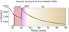 |
Fig. 1 Basic structure of the modeled CMEs. The values are extracted from a fixed location in front of the bow shock. |
3 Results
3.1 Magnetospheric structure
Here we describe the plasma environment and magnetospheric structure during the CME event. In Fig. 1 we show for reference a CME velocity profile at a fixed location in front of the bow shock, letting time evolve, to illustrate the different regions and their names discussed throughout this paper. We additionally show profiles of all plasma quantities in the Appendix B, Fig. B.1.
Cross sections through the xz-plane for DP and FR model runs are displayed in Figs. 2 and 3 respectively. Planetary magnetic fields weaker than Bp = 0.05 G do not withstand the CME’s forcing and the magnetopause is compressed to the planet’s surface. From Bp = 0.05 G to Bp = 0.21 G the pre-CME magnetosphere has larger sizes, from about Rmp = 1.4 Rp (Bp = 0.05) to nearly Rmp = 2.6 Rp (Bp = 0.21). There are no significant differences in the magnetosphere compression between DP and FR CMEs due to the high kinetic energy flux contained in both CME models. However, a major difference is the magnetic field structure of the FR CME, where an axial component (i.e., z-component) is added to the CME. The stellar wind magnetic field is nearly radial (i.e., parallel to the flow). The CME front compresses the stellar wind field and tends to align it with the shock front, visible in Fig. 2. This gives the otherwise radial stellar wind field a dominant z-component (i.e., roughly parallel to the planet’s magnetic moment), which facilitates reconnection between stellar wind and planetary magnetic field. Flux rope CMEs have a purely axial magnetic field in the center with magnetic field components becoming toroidal (i.e., within the x–y plane) toward the FR boundary. In Fig. 3 it is visible how the magnetic field’s z-component increases as the FR center approaches the planet. This enhances the reconnection efficiency between ambient and planetary magnetic field. Magnetic energy released due to reconnection at the downstream magnetopause accelerates plasma toward and away from the planet. This can be seen in Figs. 2 and 3 indicated by high velocities in the planet’s plasma shadow at roughly x > 2 Rp where stream lines diverge. This is best visible for strong magnetic fields like in the Bp = 0.21 G case, as those store more magnetic energy when the field is strongly perturbed (e.g., right panels of Fig. 3).
We tracked the upstream magnetopause position during the CME event to examine the mechanical and magnetic forcing on the planetary magnetosphere. First we extracted magnetic field profiles along the x-axis for all times. In our simulations, the magnetic field of the CME that piles up within the CME shock is mostly anti-parallel to the z-axis. From the magnetic field profiles we extracted the position of the magnetopause by determining the position of the reversal of the magnetic field and jump in its magnitude. This method yields sufficiently precise results. Magnetopause location time series for DP and FR model runs are displayed in top and bottom panels of Fig. 4, respectively. We note that the small jumps in Fig. 4 are due to the grid resolution. For all planetary magnetic field strengths considered the CMEs compress the magnetopause to Rmp = 1-1.3 Rp. For magnetic fields below Bp = 0.05 G the magnetopause is pushed to the planetary surface (see also Figs. 2 and 3). Even in the strong magnetic field case (Bp = 0.21 G) the magnetopause location drops from approximately 2.5 Rp to about 1.25 Rp. The CME sheath region (i.e., the region between the shock and the CME peak, Fig. 1) exerts the strongest forcing on the magnetosphere due to maximum total pressure. It starts after the shock crossing at 32 minutes and lasts for about 10 minutes.
In all simulations, the magnetosphere undergoes a structural change that remains as long as the CME decays. After the CME main phase a new temporary equilibrium between magnetospheric and CME pressure is reached. During the CME decay phase a tail of diluted low plasma density follows the CME and accordingly decreases the CME kinetic energy while the velocity and magnetic flux density mostly decayed to the steady state values. Consequently the magnetosphere inflates during the CME decay phase.
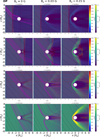 |
Fig. 2 Density pulse model results. The xz-plane cross sections are centered at Trappist-1e (see Sect. 2). Positions are given in planetary radii. Arrows depict velocity vectors and their colors velocity magnitudes (left color bar). Contours indicate plasma density (right color bar). Black and magenta lines indicate interplanetary and planetary magnetic field lines projected onto the xz-plane, respectively. We display the cross sections before the CME shock (top), during the shock crossing (upper middle), during the shath (bottom middle) and during the CME peak (bottom). Each column is for a specified intrinsic magnetic field strength, Bp. |
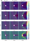 |
Fig. 3 Same as Fig. 2 but for the for the FR model. Because of a slightly enhanced CME size due to the FR magnetic pressure the CME shock crossing occurs approximately 30 s later compared to the DP case. |
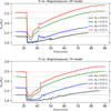 |
Fig. 4 Upstream magnetopause locations (in planetary radii Rp) of Trappist-1e for a planetary field with surface strength Bp = 0.03, 0.05, 0.15, and 0.21 G as a function of time. The upper and bottom panels display the DP and FR model runs, respectively. |
3.2 Magnetic variability and interior Joule heating
Alongside the structural change of the magnetosphere due to the CME impact, temporal magnetic field variability near the planet is generated by the plasma interaction. Varying magnetic fields B˙ induce eddy electric fields in the planetary subsurface by virtue of electromagnetic induction. The resulting electric fields drive electric currents j within electrically conductive layers. These induced currents within the planetary subsurface give rise to energy dissipation through Joule heating when electric conductivity is finite. We followed the modeling approach of Grayver et al. (2022) and defined the total Joule heating rate within the planetary body as
 (17)
(17)
where T is the duration of the CME event, V is the planetary volume, t0 and t1 are the start and end times of the integration, and E is the electric field.
To solve Eq. (17), we first need to describe the magnetic field variability at the planetary surface. In order to do so we extracted vectorial magnetic field maps directly above the planet’s surface during the CME event and decomposed the external field (e.g., the magnetic field without the constant dynamo magnetic field) for each step up to the quadrupolar degree (l = 2) using spherical harmonics multipole expansion. We also considered higher degree spherical harmonics which, however, have negligible amplitudes and thus also negligibly contribute to interior heating. This decomposition is valid for potential fields within the upper non-conducting subsurface but we only have access to magnetic field components above the surface. We validated that the magnetic field directly above the surface can be approximated well as potential field by directly comparing the magnetic field at the inner boundary and the unperturbed magnetic field transmitted into the domain by the boundary conditions. The coefficients of the multipole expansion of the field give us information about which magnetic field mode (e.g., dipolar or quadrupolar) that is generated by the interaction is dominating the magnetic field variations at the surface of the planet. We calculated the external Gauss coefficients,
 (18)
(18)
where  is the Schmidt semi-normalization factor,
  are the associated Legendre polynomials of degree l and order m. The radial magnetic field components Br as a function of colatitude θ and longitude λ were extracted from the simulations. We note that this process was done in post-processing and thus induction in the interior did not couple back to the space environment. The calculations and steps done to obtain interior Joule heating rates are summarized in Fig. 5.
External Gauss coefficient time series are shown in Fig. 6 for Trappist-1e with magnetic fields of Bp = 0, 0.03, 0.07 and 0.21 G and CME-associated flare energy of 1031 erg. For simplicity we omit Trappist-1b in this discussion due to the similarity of the magnetic fields’ dynamical behavior (i.e., the physical behavior is the same but differs only in magnitude).
Flux ropes have spatially inhomogeneous magnetic fields (see, e.g., Fig. B.1), and when convected on the planet, they cause time-variable fields near the surface. Density pulse CMEs on the contrary have approximately constant magnetic fields but carry more mechanical energy than FR CMEs due to plasma density enhancement. This incident mechanical energy, i.e., kinetic energy, compresses the planetary upstream magnetic field, which is the main source of magnetic flux variability observed in the DP model results.
In DP CME simulations, magnetic variability is dominated by the  (vertical dipole mode) and
  (equatorial quadrupo-lar mode) coefficients. The decrease of
  corresponds to an increase in north-south magnetic flux density due to magnetosphere compression. The increase of
  is associated with equatorial magnetic field components with minima at the flanks, sub- and anti-sub stellar point. As we increase the planetary magnetic field strength, these coefficients enhance accordingly until reaching the maximum near 0.04 G for Bp ≥ 0.07 G. This behavior is indicative of increasingly more efficient induction in the magnetosphere due to the stronger field. In the Bp = 0 G case there is only a slight increase of the
  coefficient that is due to stellar magnetic field draped around the planet. There are small fluctuations in the
  component most pronounced in the Bp = 0 G case relating to flow instabilities at the flanks of the planet. Variability in
  and
and  scales with Bp due to the enhanced inductive response of the plasma in the planet’s space environment (Eq. (4)).
In FR CME simulations with a non-magnetized planet, the dominant Gauss coefficients are  and
and  . The increase and decay of
  around 40 minutes directly correlates with the magnetic flux density profile along the FR with its maximum north-south component at the FR axis (Fig. B.1). Similarly, the change of the twisted FR horizontal field components (within the xy-plane) is reflected in the sinusoidal variation of equatorial
  coefficient. The equatorial field component of the FR in the xy-plane (
 ) translated to the planet decreases in strength as the compression of the magnetosphere gains in effectiveness (
 ,
,  ). Therefore, with strong planetary magnetic fields, the FR magnetic field is more efficiently shielded off by the planet’s field, and both types of CMEs nearly produce the same Gauss coefficients dominated by magnetosphere compression.
The time series of the external Gauss coefficients were used as input for the interior induction heating model of Grayver et al. (2022) where electromagnetic induction and resulting Ohmic heating was calculated for each Gauss coefficient separately. For the whole CME duration we calculated the Joule heating rate within the whole planetary volume V, QJ, for all modes according to Eq. (17) (Grayver et al. 2022). The integration was performed from start t0 to end t1 of the CME event and the result was divided by the CME duration T = 1 h. With Eq. (17), we then obtained the heating rate during a 1-hour CME event. We refer the reader to Grayver et al. (2022) for a detailed description of the induction heating model. We used a simple homogeneous interior model with a constant electrical conductivity of σ = 0.01 S/m which corresponds to the typical conductivity in the Earth’s asthenosphere and lower lithosphere (Naif et al. 2021). This choice was motivated by the proposed interior composition of the Trappist-1 planets similar to that of Earth (Agol et al. 2021). The likely enhanced electrical conductivity at larger depths does not have a strong effect on our assumption of constant conductivity σ = 0.01 S/m because currents attenuate with depth due to the skin effect. Most heating occurs in the uppermost layers of the planets in depths up to a few hundred kilometers where electrical conductivity may be approximated to first order as spatially constant.
The dissipation rates QJ in the interior of Trappist 1b and e for one CME with Eflare = 1031 erg are shown in Fig. 7. In the Bp = 0 G scenario, we find a heating rate averaged within 1 hour of approximately 0.01 TW (Tr-1e) and 0.1 TW (Tr-1b) in the DP case. CMEs expand during their propagation through the heliosphere, and therefore the energy density decreases accordingly. Because of that Trappist-1b experiences stronger CMEs, resulting in higher QJ as magnetic perturbations enhance with incident energy. For both CME models, heating rates reach up to 1–2 TW at Bp = 0.09 G for Trappist-1e. The maximum heating lies outside our parameter space for Trappist-1b but QJ flattens toward the maximum BP = 0.21 G of this study toward around 20 TW.
Our calculations show that for the FR CMEs the dissipation QJ is only very mildly dependent on the strength of the internal field Bp (see Fig. 7). It typically increases as long as Bp is small until 0.1 G and then maximizes or goes into saturation. This is very different for the DP CMEs. The electromagnetic dissipation strongly increases with the strength of the planetary field up to 0.1 G. The reason is that a stronger Bp enables a stronger generator mechanism to convert the mechanical energy of the CME into electromagnetic energy dissipated within the planet. Above Bp = 0.05 G (Tr-1e) and ≈0.15 G (Tr-1b) heating rates in both CME models have the same functional dependence on Bp as magnetic variations intrinsic to FR CMEs are increasingly shielded off by the planetary magnetic field (see also Fig. 6).
Interior heating rates for Trappist-1e with the atmosphere considered here are similar to those without such an atmosphere. However, for weak magnetic fields Bp < 0.1 G heating rates are slightly enhanced in the FR CME case. An atmosphere weakens the plasma flow near the planet. Therefore, mechanically generated perturbations are damped accordingly, resulting in a slightly lower inductive response in the planetary interior. The increase in heating rates in the FR case (Bp < 0.1 G) comes from enhanced tension on the reconnected field lines, since the motional response of magnetospheric plasma to external forcing is counteracted by the atmosphere that acts as energy sink.
The majority of dissipated energy presented here is dissipated only within the uppermost layers of the planets. This is due to the exponential attenuation of magnetic fields with depth caused by the skin effect.
To further study the effect of the interior electric conductivity on Ohmic dissipation, we additionally calculated heating rates with conductivities between 10−9 to σ = 0.1 S/m (Fig. 7). As the maximum heating rate in the Tr-1e model is achieved at Bp = 0.11 G we only show the maximum heating rates as a function of the electrical conductivity in Fig. 8. In Fig. 8, we see that dissipation maximizes at intermediate conductivities around 10−4 S/m. Therefore, a lithosphere conductivity comparable to that of Earth already produces maximum heating rates in our model. More insulating as well as more conducting lithospheres lead to a lower Ohmic dissipation.
Lastly, we note that we also examined the effect of CME duration on heating rates. For durations T >> 1 h heating rates approach a lower limit approximately a factor of < 2 smaller than those presented here for T = 1 h. The effect of CME duration on interior heating is thus, according to our model, insignificant. (See Appendix C for a discussion on this conclusion.)
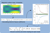 |
Fig. 5 Schematic of the post-processing pipeline to calculate the CME-induced Joule heating in the interior of a planet. |
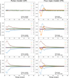 |
Fig. 6 Evolution of the external Gauss coefficients (Eq. (18)) during one CME as a function of time (minutes) for planetary magnetic field strength: Bp = 0 (top), 0.03 (upper middle), 0.07 (lower middle), and 0.21 G (bottom). The left column shows DP; the right column shows FR model results. Displayed are all considered external Gauss coefficients ( |


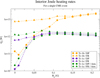 |
Fig. 7 Joule heating averaged within 1-hour CME events in the interior of the planets, QJ (Eq. (17)), given in Watts as a function of planetary magnetic field strength, Bp. Triangles denote FR, circles DP CME cases. Yellow data points correspond to Trappist-1e, purple to Trappist-1e. Green data points denote the results with an atmosphere around Trappist-1e. |
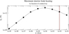 |
Fig. 8 Heating rates at Bp = 0.11 G for Trappist-1e as a function of the electric conductivity, σ, in S/m. The brown vertical line indicates the homogeneous model conductivity adopted in this study. |
3.3 Ionospheric Joule heating
In addition to interior Joule heating, energy is also dissipated in the ionosphere through ionospheric Joule heating. The presence of a neutral species introduces collisions between plasma and neutral particles due to their relative motion. These collisions cause the ions to dissipate energy in form of frictional heating (Vasyliu¯ nas & Song 2005). Ionospheric Joule heating can be calculated using the convective electric field E = -v × B and the plasma conductivity perpendicular to the magnetic field, i.e. the Pedersen conductivity σP. We calculated the ion term of the Pedersen conductivity for each grid cell, which is a function of the ion-neutral collision frequency, νc; ion gyro frequency, ωg; and ion number density, ni (Baumjohann & Treumann 2012):
 (19)
(19)
Here, e is the elementary charge, me is the electron mass, and mi the ion mass. The collision frequency is defined as in Eq. (7), and the ion gyro frequency can be calculated with ωg = eB/mi. The ionospheric Joule heating per unit volume can then be calculated with qJ,ion = σPE2. We integrated this expression over the magnetosphere volume, V, to get the total ionospheric Joule heating rate and integrated the resulting heating rates over the CME event duration. By dividing the result by the CME duration, T, we obtained the average ionospheric Joule heating rate for one CME event:
 (20)
(20)
where t0 and t1 are the start and end times of the CME event. We integrated Eq. (20) from the surface at 1 Rp to 1.5 Rp to avoid including the shock and unshocked CME plasma. We only consider magnetic fields ≥0.05 G due to the magnetopause being pushed to the planetary surface for weaker fields. Resulting heating rates are shown in Fig. 9. For DP model runs we obtain heating rates from 3 × 10⁴ TW (Bp = 0.0 G) down to 12 × 103 TW (Bp = 0.21 G) while heating rates in the FR case are approximately a factor of 2 higher. Contrary to interior Joule heating, ionospheric Joule heating rates decrease with increasing magnetic field strength, because the ionospheric Pedersen conductivity is inversely proportional to the magnetic field strength. In contrast to the interior Joule heating, the effect of Joule heating on ionospheric plasma is nearly instantaneous and about four orders of magnitude stronger. Therefore, CME-induced ionospheric Joule heating directly heats up the space plasma, which may lead to comparably severe effects on the upper atmosphere, such as atmospheric inflation and significant escape rates during CME events. In Fig. 9, we additionally show ionospheric Joule heating rates due to the steady-state stellar wind before the CME event, Q0,ion. In the non-magnetized case the dissipation rates reach up to 8 × 10³ TW and then quickly decay toward 10 TW as we increase the planetary magnetic field strength. Thus, a CME enhances ionospheric dissipation rates by one to two orders of magnitude on average.
To put these dissipation rates into context, we estimate the amount of stellar XUV power received by the dayside of Trappist-1e. XUV flux is the main driver of photo-evaporation and thus has a severe impact on the survivability of planetary atmospheres. Modeling studies based on observations from Wheatley et al. (2017) suggest that the XUV luminosity LXUV of Trappist-1 has saturated at a value of about LXUV/Lbol ≈ 10−3 during a large part of the star’s lifetime (Birky et al. 2021; Fleming et al. 2020). We took this value as the upper limit XUV luminosity and the bolometric luminosity of Trappist-1, Lbol = 5.5 3 × 10⁴ L⊙ (Ducrot et al. 2020). We then calculated the total XUV power received by the dayside of Trappist-1e of QXUV = 9.5 × 101 TW. Additionally, we used the XUV flux from the MEGA-MUSCLES spectrum (Wilson et al. 2021) to also estimate the XUV power on the dayside of Trappist-1e similar to Strugarek et al. (2025). The resulting XUV power is QXUV = 1.64 × 10² TW. We display the upper limit XUV power estimate in Fig. 9 for comparison with the ionospheric Joule heating rates.
According to our estimates and model results, the planet approximately receives the same amount of XUV power and steady-state ionospheric Joule heating power, QXUV ≈ Q0,ion, for Bp > 0.1 G. During a CME event; however, dissipation rates in the ionosphere quickly increase by one to two orders of magnitude, depending on the planetary magnetic field. The fast response of ionospheric plasma to heating rates on the order of 100–1000 TW possibly results in severe atmospheric escape during CME events which makes close-in planets around active stars less likely to retain their atmospheres as they receive this energy in addition to flare XUV fluxes and stellar quiet XUV radiation. We note that our calculated dissipation rates are time-averaged over the duration of the CME and that peak heating during the CME main phase exceeds the presented values considerably.
Lastly, we note that the ionosphere may shield the planetary surface from external magnetic variations due to the skin effect (e.g., Strugarek et al. 2025). However, for this shielding to be effective, large ionospheric conductances and a high frequency of magnetic variability are needed to decrease the skin depth to lower values compared to the extent of the ionosphere. By height-integrating the Pedersen conductivity (Eq. (19)) in our simulated ionospheres we find the Pedersen conductance to be approximately 5–20 S in more strongly magnetized cases (from about 0.05 G) and up to 600 S in the weakest magnetic field case. With the frequency of magnetic variability on the order of one minute we find the skin depth for moderately to strong magnetized planets to be on the order of hundred kilometers. This poses lower limits since the period of magnetic variability in our simulations is considerably longer (see Fig. 6). In the weakest magnetic field cases the skin depth decreases toward tens of kilometers. Therefore, in the case of efficient magnetic screening, the energy dissipated in the ionosphere would increase significantly. However, most importantly our study shows in case of a conductive ionosphere, that the overall dissipation rate in the ionosphere can be orders of magnitude larger compared to the dissipation due to induced fields in the interior. Thus, additional shielding in the ionosphere only further increases the dominance of the ionospheric heating.
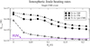 |
Fig. 9 Ionospheric Joule heating rates (Eq. (20)) averaged within 1 hour CME events for Trappist-1e as a function of planetary magnetic field Bp. The DP and FR model results are denoted by circles and triangles, respectively. The dayside XUV power received from the star is also indicated. |
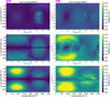 |
Fig. 10 Maps of time-averaged magnetic variability, dB/dt (nT/s), of the radial magnetic field component obtained directly above the planetary surface. Co-latitude and longitude are shown on the Y and X axes, respectively. Upstream direction is at longitude below 180 degrees. Model results are shown in the left column for the DP and in the right column for the FR case. We show maps for Bp = 0 (top), 0.05 (middle) and 0.15 G (bottom). |
3.4 Localization constraints on interior heating
Induction driven interior Joule heating is proportional to the temporal change of magnetic flux, i.e. Q ∞ dB/dt whereas only the radial component of the magnetic field is required to assess Q (see Eq. (18)). The plasma interaction between planet and space environment is fundamentally asymmetric since the orientation of the magnetic field and the ambient plasma velocity field are key variables that deform and align the magnetosphere with the flow and ambient magnetic field. In Fig. 10, we show maps of time-averaged radial component of |dB/dt| over the surface of Trappist-1e with several planetary magnetic field strengths. The trends we describe in the following are also observed in Trappist-1b simulations. We therefore omit these results for simplicity.
If the planet is non-magnetized most dB/dt is found downstream near the equator due to the high tension on the stellar wind and CME magnetic field lines within the wake of the planet. In the FR scenario dB/dt is generally more homogeneously distributed. As we switch on the planetary magnetic field we observe the average dB/dt to increasingly focus at the upstream hemisphere near the polar cusps due to the planetary magnetic field lines being mostly radial there. For planetary magnetic fields Bp ≤ 0.07 G, the average dB/dt in the FR scenario are more widely distributed and washed out over the upstream hemisphere. For stronger planetary magnetic fields the distributions of dB/dt in both CME models become increasingly similar. The average dB/dt peak in both CME scenarios at planetary magnetic fields of Bp ≈ 0.11-0.15 G. Afterward, the dB/dt decay slightly but remain focused in the upstream polar regions.
These results suggest that the degree of local focusing of the heating correlates strongly with the planetary magnetic field strength. Stronger magnetic fields favor CME-induced interior heating to peak on the upstream hemisphere at high latitudes.
4 Discussion
In this section we aim to better understand the electromagnetic energy fluxes around the planets and how they relate to CME-induced interior heating. We first discuss the energetics of the CME-magnetosphere interaction in Sect. 4.1. We discuss the time variability of near-surface Poynting fluxes during the CME event and assess the energy transfer from CME to the magnetosphere (Sect. 4.1.1). In Sect. 4.1.2, we consider time averaged Poynting fluxes, compare them to interior Joule heating and study the scaling of input power near the surface as a function of planetary magnetic field strength. In Sect. 4.2, we briefly discuss the dependence of interior heating on CME-associated flare energy.
4.1 Energetics of the CME-magnetosphere interaction
Magnetic variability is mostly controlled by electromagnetic energy propagated by Poynting fluxes. In our model these Poynt-ing fluxes are generated by the CME-planet plasma interaction and ultimately deliver the electromagnetic energy to the planet’s surface where it is, to some extent, dissipated by Joule heating. We distinguish between two regimes of electromagnetic energy transfer. The closed field line region (i.e., the magnetosphere) is defined by all planetary magnetic field lines that intersect the planet’s surface twice. Here magnetic energy is propagated mostly along field lines. The open field line region is defined by highly mobile magnetic field lines that originate in the planet and connect to the stellar magnetic field. Energy and mass of the stellar wind and CME are injected into the magnetosphere across the open magnetic field. Magnetic energy transport in this regime is dominated by convection.
Figure 11 shows a schematic illustrating magnetic variability and associated Poynting fluxes. Before the CME the planetary magnetic field B0 is in equilibrium with its surroundings. This perturbed dipole is compressed on the upstream side and elongated on the downstream side (e.g., top panels of Figs. 2 and 3). A CME or any variation in the interplanetary medium perturbs the steady-state field toward a new, temporary equilibrium magnetic fields B1. The perturbation magnetic field δB (i.e., the residual field B1 - B0) drives Alfvén waves perpendicular to δB which propagate the magnetic variability, dB/dt, parallel to B1 with Alfvén velocity vA toward the planet as well as away from it. These Alfvén waves carry electromagnetic energy that is associated with Poynting fluxes S|| parallel to B1. The parallel Poynting flux can be calculated using the residual magnetic and associated electric field,
 (21)
(21)
where the velocity  is the Alfvén velocity (Saur et al. 2021, 2018; Park et al. 2017; Saur et al. 2013; Keiling 2009). The maximum dB/dt can be expected where B1 is perpendicular to the surface of the planet, |B1| ≈ Br (i.e., the field lines are purely radial) so that S|| ≈ Sr.
In Fig. 12, we show a map of Sr directly above the surface of Tr-1e. Only Poynting fluxes toward the planet are shown, resulting in the negative signs. The red line denotes the open-closed field line boundary (OCFB). For latitudes below the OCFB the field lines are closed. The OCFB shown here is similar in all magnetic field as well as CME models and changes only minimally during the CME event. Figure 12 shows that almost all Poynting fluxes Sr lie within the closed field line region, indicating that the electromagnetic energy parallel to the magnetic field is generated almost exclusively within the closed magnetosphere due to magnetosphere compression. The field lines near the OCFB are most mobile in the sense that they are convected downstream by the external plasma flow. Given the magnetic variability maps in Fig. 10 we expect the magnetic variability to be mostly transported along magnetic field lines, and the distribution of Sr within the OCFB supports this. We also show Sr maps for Bp = 0.05, Bp = 0.15 and Bp = 0.21 models during the CME main and decay phase in Fig. D.1 to illustrate the general dominance of Sr in regions where most magnetic variability (i.e., dB/dt, Fig. 10) is found independent of the CME model. Furthermore, the Poynting flux distribution near the CME peak (middle column) correlates best with the magnetic variability maps, indicating that most heating might be generated during the CME sheath and not during the shock crossing (see also Fig. 1).
Due to these considerations, we focus our analysis in the following sections on the electromagnetic energy that is delivered inward by radial Poynting flux components, Sr. We formulated the integrated Poynting flux as integral over radial Poynting fluxes directed toward the planet,
 (22)
(22)
where Aplanet is the surface area of the planet and Sr− are the radial components of the Poynting flux directed toward the planet. Due to the spherical coordinate system, the inward flux is negative. Therefore, we omitted the sign and indicate the inward components with the minus superscript. In the following sections we use Sin− to study the temporal evolution of interaction-generated magnetic variability as a function of the CME model and time and how planetary magnetic fields affect the transfer of magnetic energy toward the planet surface.
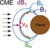 |
Fig. 11 Sketch illustrating the generation of the background magnetic field aligned Poynting fluxes associated with Alfvén waves. We do not show fast mode waves due to the negligible effect on the radial components of near-surface magnetic variability, dB/dt, found with our model. |
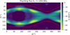 |
Fig. 12 Open-closed field line boundary (red lines) plotted on top of an inward Poynting flux, Sin, map for Trappist-1e, Bp = 0.21 G, DP model. As an example, the map is shown during the CME sheath crossing, but the boundary remains almost constant over the entire simulation period for DP as well as FR simulations. |
4.1.1 Magnetospheric Poynting fluxes during the CME
The upper panels of Fig. 13 show integrated Poynting fluxes as defined in Eq. (22) for Trappist-1e during the CME event. We show results for planetary magnetic field strengths of Bp = 0.03, 0.05, 0.09, 0.11 and 0.21 G.
The CME shock hits the magnetosphere at about 32 minutes and is followed by a sheath region where plasma density, pressure, and magnetic flux density are strongly enhanced (see also Fig. 1 for a description of the general CME structure). The sheath crossing ends at approximately 42 minutes with DP CMEs and slightly delayed (1–2 minutes) with FR CMEs. Inward Poynting fluxes rapidly increase by 1 to 2 orders of magnitude with the shock hitting the magnetosphere. For planetary magnetic fields from Bp = 0.05 G and stronger  reach powers of 1015−16 W.
  increase with increasing Bp, the differences, however, become small for Bp > 0.05 G. We note that above Bp = 0.05 G the magnetospheres always have magnetopause radii greater than Rp, and thus magnetosheath dynamics do not contribute directly to the calculated Poynting fluxes. In DP and FR simulations we observe an oscillatory evolution of
  during the first 4 minutes after the shock intercepts the magnetosphere. During this time, the CME-induced compression and strong magnetic pressure of the compressed planetary magnetic field counteract each other periodically.
In both models, the total CME energy flux decays following the exponential decrease of the initial CME profile that is stretched and therefore diluted along the flow direction due to the fast CME front. The magnetopause radius increases due to the decreasing CME ram pressure of the diluted CME tail plasma (Fig. 4). The stronger Bp, the slower is the decay of  due to the larger area to intercept CME energy.
For all models, strongest Poynting fluxes are generated during the CME sheath and peak crossing with  amounting to 1015-16 W in a time span of about 10–15 minutes. The convected Poynting flux clearly depends on Bp, whereas the dependence becomes stronger when Bp ≥ 0.09 G. From the beginning of the CME event up to the decay phase (50–90 minutes)
  drops by approximately one order of magnitude.
Transfer of energy fluxes We calculated the CME kinetic energy flux, Pkin; thermal energy flux, Pth; and the Poynting flux, SCME, of the plasma incident on the magnetospheric cross section,  :
:
 (23)
(23)
 (24)
(24)
 (25)
(25)
where v denotes the CME plasma velocity, v⊥ the velocity perpendicular to the magnetic field, n the plasma number density, T the temperature and B the magnetic flux density. All these parameters were obtained directly in front of the magnetosphere where the CME plasma is not yet perturbed.
We compared the incident CME Poynting flux with  by calculating the Poynting flux ratio,
 (26)
(26)
We note that ϵS is not an efficiency factor (that must be ≤ 1) but a fraction that allows us to get an idea of the amount of  that is generated within the magnetosphere due to magnetic field perturbation (i.e., if ϵS > 1). Additionally, following Elekes & Saur (2023), we calculated the transfer function between total incident energy flux (Eqs. (23)–(25)) and
  ,
,
 (27)
(27)
The transfer function measures the conversion efficiency of incident energy to magnetospheric inward Poynting fluxes. As ϵT relates the total available energy to magnetospheric Poynting fluxes it must be smaller than unity. Together, both quantities may be used to assess the interaction strength and to identify energy transfer that occurs due to mechanical interaction or via reconnection and convection. In the middle and bottom panels of Fig. 13 we show the time series of ϵS and ϵT, respectively.
In DP model runs,  exceeds the incident Poynting flux by several orders of magnitude. During the CME shock crossing, ϵS increases for all Bp by two orders of magnitude up to 103. These high ϵS indicate a high amount of
  generated by conversion from CME mechanical to magnetic energy (i.e., by magnetosphere perturbation). The transfer function ϵT reaches a maximum value of 0.4 during the shock crossing in the Bp = 0.21 G case and about 0.2–0.3 for Bp ≈ 0.05 G. Afterward, ϵT is reduced to 0.1 and 0.2, indicating a slightly lower efficiency of CME energy injection. We thus identify magnetosphere compression to be the dominant mechanism for DP CMEs which is supported by most dB/dt occurring near the polar cusps (Fig. 10, left).
In FR model runs, we observe a different behavior of the energy transfer. ϵS is significantly lower, between 1 and 60, since magnetosphere compression also occurs in this scenario due to the high velocity of the CME. ϵT is generally higher compared to the DP scenario and lies between 0.1 and 0.7. This is due to the strong intrinsic magnetic variability and thus the Poynting flux already contained within the FR that dominates the total energy flux. Smaller ϵS during the FR passing indicate that less magnetic energy is released due to a mechanical interaction. This becomes clearer when focusing on the CME sheath and peak passing, where, nearly for all Bp, ϵS falls to values between 0.5 and 3 while ϵS is smaller for weaker Bp, which is supported by the QJ scaling with weak Bp in Sect. 3.2. This is indicative for dominant Poynting flux and thus magnetic variability transfer along open field lines due to reconnection. This transfer of magnetic variability is the root cause for the persistent heating efficiency seen in Fig. 7. If no or a weaker planetary magnetic field is present, the magnetic generator mechanism (Eq. (4)) that converts motional energy into magnetic energy (i.e., dB/dt) is not existent or weaker, respectively. For stronger Bp ≥ 0.05 G magnetic energy released due to compressional perturbation increases, raising ϵS to 2–3.
After the CME peak at about 43 minutes, ϵS drops off slowly in the DP CME case as the mechanical energy of CME slowly decays in the CME tail. In the FR scenario ϵS shows slight variations due to the FR’s twisted magnetic field structure slowly breaking down to eventually approach the steady-state magnetic field configuration of the stellar wind. For the weaker planetary magnetic field regime (Bp ≤ 0.11 G), ϵT remains fairly constant at 0.1. In the CME tail region, density and velocity drop to minimum values, and at the same time, Rmp rises (Fig. 4). The magnetosphere reacts increasingly sensitive to variations in the ambient plasma like density, velocity and magnetic field gradients across the CME tail when the magnetosphere’s effective size increases.
In summary, we found evidence for a strongly enhanced CME Poynting flux-to-magnetospheric Poynting flux transfer if the CME possesses a FR. Mechanically dominated CMEs convert only a small fraction, ϵT ≤ 0.2 (0.4 peak during shock crossing), of the total energy flux to inward Poynting fluxes above the planet’s surface. Flux rope CMEs already contain large Poynting fluxes, but get them also well into the magnetosphere. With the total energy flux dominated by magnetic energy, the fraction of total energy transferred to magnetospheric Ponyting fluxes increases considerably with Bp and reaches up to 0.7. To put this value into context, in a steady state stellar wind scenario we found the transfer efficiency to be approximately 0.15–0.2 for the magnetosphere of τ Boötis b (Elekes & Saur 2023).
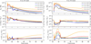 |
Fig. 13 Time series of |

4.1.2 Scaling behavior of magnetospheric Poynting fluxes and the role of planetary magnetic field strength
We are interested in understanding the functional dependence of  on Bp and thus how planetary magnetic fields affect the Poynting flux above the planet’s surface. We averaged
  over the CME duration and display it as a function of Bp for Trappist-1b and e (Fig. 14). Despite the Poynting fluxes varying over orders of magnitudes during the CME event, the average Poynt-ing flux nevertheless quantifies the average energy injected into the magnetosphere during the event. Contrary to the heating rates in Fig. 7 the averaged Poynting fluxes do not have a maximum within our parameter range.
In general, we find that the Poynting flux  always increases with the planetary magnetic field strength Bp. In the Trappist-1b case
  increase from about 1013 W to 5 × 10¹⁵ W (DP) with the magnetic field Bp while in the FR case the Poynting fluxes exhibit a lower limit of 5 × 10¹⁵ W. For Trappist-1e the Poynt-ing fluxes are significantly reduced by approximately an order of magnitude, while the behavior of
  as function of Bp is similar to Trappist-1b. As the external forcing (i.e., the CME) is kept constant, this scaling of Poynting fluxes with the intrinsic magnetic field illustrates that stronger fields are capable of absorbing and converting more electromagnetic energy so that the electromagnetic shielding capability of intrinsic magnetic fields is reduced when they become stronger.
We then fitted  with respect to Bp (Fig. 14). The results in Fig. 14 suggest that inward Poynting fluxes above the planet’s surface scale mainly with Bp following a cubic power law. Effectively
  scales with B3p indicating that stronger intrinsic magnetic fields enhance the magnetosphere’s intake of external electromagnetic energy.
In Fig. 14, we also display the ratio of Qj to  as green, dashed line to assess how the radial Poynting fluxes translate to interior heating as they supply the planetary surface with the majority of magnetic variations. The Poynting flux-to-interior heating efficiency for magnetic fields above 0.05 G is largest for Trappist-1b, approximately 2-3 × 10⁻³, and is slightly reduced for Trappist-1e with approximately 10−3. The efficiency slightly decreases toward an Earth-like magnetic field strength. Peak Poynting flux-to-interior heating efficiencies are found at magnetic field strengths between 0.5 and 0.11 G.
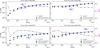 |
Fig. 14 Time-averaged inward Poynting fluxes |


4.2 Interior heating as a function of CME-associated flare energy
For our basic model, we considered a flare bolometric energy of 1031 erg. Flares of this energy occur on average once per day according to the recent flare frequency distribution of Howard et al. (2023). Here we address the question of how interior heating relates to flare energy. For this purpose we additionally considered flare energies of 1029, 1030, 1032 and 1033 erg which all reside in a reasonable energy range for Trappist-1 (Howard et al. 2023). We ran our MHD model with CMEs based on these flare energies (see Sect. 2.4 for our CME models and Eqs. (9), (10) and (15) for flare-CME scaling laws). Unfortunately, we were not able to run the same MHD model for more energetic CMEs (Eflare ≥ 1034 erg) due to limitations of the numerical method. The CME duration is kept at 1 hour. In Fig. 15, we show resulting heating rates as a function of flare energy in erg. For simplicity we only consider Trappist-1e with magnetic fields of Bp = 0.01, 0.05, 0.11 and 0.17 G. We also show the CME total energy density as a function of flare energy.
For CMEs dominated by mechanical energy (DP), QJ depends relatively weak on flare energy. Heating rates increase by less than an order of magnitude within our flare energy range in the DP case (Fig. 15a). In the non-magnetized planet case, QJ can be considered nearly independent of flare energy since no considerable magnetosphere exists that could act as generator to convert the CME mechanical energy to magnetic energy. With increasing magnetic field strength the magnetospheric generator action enhances and so does the converted magnetic energy that ultimately drives induction in the interior. For CMEs dominated by magnetic energy (FR) the dependence of interior heating rates on flare energy is fairly equal for all considered planetary magnetic fields, as magnetic energy is already contained within the CME and no efficient generator mechanism is needed (Fig. 15b). In general, QJ(Eflare) follows the increase in incident energy density of FR CMEs with flare energy more closely than in the DP case.
In comparison to the results of Grayver et al. (2022), our interior heating rates show a weaker functional dependence on flare energy due to the plasma interaction added to the model. When a planet is magnetized, CME energy is never directly transferred toward the planet. A large portion of dB/dt above the planetary surface is produced by induction in the magnetospheric plasma with a certain efficiency, which increases with planetary magnetic field strength (see Sect. 4.1.1). The magnetospheric generator is driven by the CME’s mechanical energy and the resulting perturbation of the planetary magnetic field.
In the weakly magnetized planet case with Bp = 0.01 G, however, our FR scenario results (Fig. 15b) fit well within the distribution of heating rates obtained by Grayver et al. (2022) since the magnetic energy of the FR is nearly directly supplied to the planet’s interior due to the lack of a significant magnetospheric generator. In the Bp = 0.01 G case, above Eflare = 1031 erg, QJ(Eflare) assumes the functional dependence of the stronger magnetized scenarios (Fig. 15b). We account this to the energy partition of the CME kinetic and magnetic energies. The CME velocity grows slower with flare energy compared to the FR magnetic field strength (see Eqs. (9)–(10) and (15)–(16)). From Eflare = 1030 erg to 1033 erg the CME velocity enhances by a factor of 1.5 while the FR magnetic field strength by 18. Therefore, by decreasing Eflare toward 1029 erg, we quickly reach a kinetic energy dominated regime in which the generation of dB/dt mostly depends on the magnetospheric generator action, and thus QJ (1029erg) is nearly the same in the DP and FR scenario.
In summary, in the DP case, QJ depends less strongly on Eflare when the CME is dominated by mechanical energy. The increase of QJ with flare energy enhances with stronger planetary magnetic fields. For CMEs with a magnetic FR structure. However, we find a moderately strong dependence that is constant for all intrinsic magnetic fields above approximately 0.03 G.
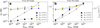 |
Fig. 15 Time-averaged interior heating rates as a function of CME-associated flare energy Eflare (erg) for DP (a) and FR (b) CMEs. We only show heating rates for Bp = 0 G (black circles), Bp = 0.05 G (blue upward triangles), Bp = 0.11 G (green downward triangles), and Bp = 0.17 G (yellow diamonds). Gray triangles denote the incident total energy flux of the CME (right y-axis). |
4.3 Long-term interior Joule heating rates
Using the flare frequency distributions of Trappist-1 and analogue stars (Howard et al. 2023; Seli et al. 2021) together with single-event Joule heating rates for different CME-associated flare energies (Sect. 4.2, Fig. 15) we estimated the time-averaged heating rate over one year with several different CME events. Given the average number of flare events per day nE(Ei) for a given flare energy Ei taken from Howard et al. (2023) we can estimate the average number NE of flares per year for each flare energy, NE = nE · 365 (see Table 3). We divided the flare energy range into logarithmically spaced energy bins, Ei ∈ [1029,1030,1031,1032,1033] erg, with i ∈ [0,4]. Single event heating rates derived with our CME model are shown in Fig. 15. The fraction of all flare events that are associated with a CME which intersects a planet is f ≈ 0.08 according to the estimate of Grayver et al. (2022). We multiplied the heating rates QE (Ei) due to CMEs with energy Ei (Fig. 15) with their corresponding number of annual events and then divided them by N = 365 days to obtain an estimate for the average annual heating rate, QCME,
 (28)
(28)
Resulting annual average heating rates are displayed in the lower box in Table 4. We also estimated the annual heating rates for Tr-1b by assuming QJ (E) having the same form as for Tr-1e (15). We scaled the fit function in Fig. 15 to match the heating rate QJ(E = 1031 erg) obtained from our basic model for Tr-1b (Sect. 3.2, Fig. 7). With QJ(E) obtained, we applied the same calculations as for Tr-1e presented in this section. We omitted the data for Bp = 0.01 G due to the substantially different functional dependence of QJ on E in this case (Fig. 15).
Large-scale stellar magnetic fields are capable of suppressing or slowing down CMEs, leading to lower energies contained in CMEs intersecting planets (see Sect. 2.5). We therefore note that the dissipation rates presented here are presumably upper limits. Annual interior heating due to CMEs is on the order of 1-10 TW for Trappist-1b and 0.1-1 TW for Trappist-1e. Comparing these results with the heating rates of Grayver et al. (2022) obtained from a homogeneous interior model, we find our heating rates to lie within the lower range of their results. We find the best agreement between our results and those of Grayver et al. (2022) for very weakly magnetized planets. Therefore, by considering a CME model incorporating time-dependent MHD simulations of the CME-planet interaction, CME-induced interior Joule heating has a tendency toward lower dissipation rates. Our heating rates for Trappist-1e are insignificant compared to the tidal heating rates estimated by Bolmont et al. (2020) which are, on average, 1–2 orders of magnitude higher. Compared to the interior heating rates due to the planet’s motion through the stellar dipole field (Kislyakova et al. 2017, corrected by Grayver et al. (2022) using a more recent stellar rotation rate), our results are roughly one order of magnitude lower. However, the results of Kislyakova et al. (2017) depend on the unconstrained tilt of its magnetic moment with respect to the planet’s orbital plane, and thus with low inclination, the resulting heating rates are lower.
Statistical flare and CME parameters.
Time-averaged annual Joule heating rates (TW) in the interior of Trappist-1b and e due to CMEs.
5 Summary
In this study, we have investigated the interaction between CMEs and exoplanets using MHD simulations. We chose Trappist-1b and e as exemplary cases and studied the resulting magnetic variability on the surface of the planets. The CME-generated magnetic variations at the surface of the planets induce electric currents in the planetary interior, which dissipate energy in the form of heat. We have developed an MHD model to simulate the interaction of DP and FR CMEs with magnetized and non-magnetized planets. With the choice of magnetically (FR) and mechanically (DP) dominated CMEs, we were able to study in detail the transfer of CME energy toward the planet’s surface separately. In this way, we were able to better understand the role of planetary magnetic fields in the conversion of energy and in governing dissipation of external energy fluxes within the planet and its atmosphere. We considered a range of intrinsic dipolar magnetic fields from Bp = 0 G to a nearly Earth-like field with Bp = 0.21 G. We derived CME parameters from flare-CME scaling laws obtained from Solar System observations and applied them to CMEs with associated flare energies from Ef lare = 1029 to 1033 erg. Our CMEs have a duration of 1 hour. We used a planetary interior model with constant electric conductivity and calculated induction heating using the model of Grayver et al. (2022). For Trappist-1e we also considered an O2 atmosphere and calculated ionospheric Joule heating during the CME event. In the following, we summarize the main results of this study:
- (1)
Taking into account the MHD processes around the planets, we find that CME induction heating in the interior is smaller and within the lower end of the heating rates previously derived Grayver et al. (2022). Within the parameter space studied here, an intrinsic magnetic field generally acts as an “enhancer” of stellar wind magnetic variability on the surface of the planets, which confirms the results of Grayver et al. (2022). Stresses on the magnetosphere are argued to be the main driver of magnetic variability at the planetary surface. For FR CMEs and with weak planetary Bp, the intrinsic magnetic variability of the CME can be directly transported to the planet’s surface. With increasing Bp, however, the magnetic energy that can be released by mechanical perturbation exceeds the magnetic energy of the FR. Interior heating due to FR CMEs is enhanced when an atmosphere is present due to additional tension imposed on the reconnected magnetic field lines;
- (2)
Ionospheric Joule heating rates range from 1-4 × 10⁴ TW for weakly magnetized planets down to 1-3 × 10³ TW toward stronger magnetic fields. Joule heating of the upper atmosphere does not rely on electromagnetic induction but directly results from the increase of magnetospheric electric fields. With this nearly instantaneous heating during CMEs atmospheric inflation and possible erosion might be drastically enhanced. CME-induced Joule heating rates in the upper atmosphere exceed the XUV radiation by one to two orders of magnitude. These large dissipation rates suggest that a single CME might have severe effects on the atmosphere of Trappist-1e and possibly similar close-in terrestrial exoplanets. Ionospheric Joule heating rates due to the steady-state stellar wind amount to ≈2 × 10² TW if the planet is strongly magnetized and up to 8 × 10³ TW without the presence of a planetary magnetic field;
- (3)
Regions on the planetary surface with strong radial dB/dt are increasingly confined to areas near the upstream polar cusps within the closed field line region for stronger planetary magnetic fields. Inward oriented radial Poynting fluxes,
 , at the planetary surface spatially coincide well with the dB/dt maxima;
 - (4)
Our results suggest that, in an electromagnetic sense, planetary magnetic fields enhance the capability of planets to receive and convert the energy injected through CMEs. The generation and transfer of field-aligned Poynting fluxes toward the planet as well as inductive coupling between magnetospheric variations and the planet’s interior correlates well with increasing intrinsic magnetic field strength. This behavior is only moderately sensitive to changes in CME energy density if the planet is at least weakly magnetized. Planetary magnetic fields do not shield the planet’s surface from electromagnetic energy received from CMEs and other bursty stellar wind variations as long as the planet does not possess a highly conductive ionosphere;
- (5)
We find a generally weak functional dependence of interior heating rates, QJ, on CME-associated flare energy within our parameter space. For DP CMEs, the dependence is almost non-existent for weak planetary magnetic fields Bp ≲ 0.01 G). For stronger magnetic fields, heating rates increase by less than an order of magnitude within our considered flare energy range. For Bp ≳ 0.1 G, the scaling seems to saturate. For FR CMEs, heating rates increase by almost one order of magnitude within the flare energy range considered. The dependence of heating rates on flare energy is approximately constant for all considered planetary magnetic fields Bp > 0.01 G. Heating rates scale strongly with Eflare for very weakly magnetized planets with Bp ≤ 0.01 G;
- (6)
From the flare frequency distribution of the Trappist-1 star, we estimated the average number of annual CME events. Together with our simulated interior heating rates due to CMEs with different flare energies, we calculated the annual average interior heating rates to be on the order of 1–10 TW (Tr-1b) and 0.1-1 TW (Tr-1e). These heating rates are approximately two orders of magnitude lower compared to the results of Grayver et al. (2022). Thus, considering an MHD model of the CME-planet interaction, we find CME-induced interior Joule heating to be less significant compared to dissipation rates obtained from purely electromagnetic models due to the highly non-linear coupling between external forcing and interior dissipation. Our estimated average dissipation rates are about two orders of magnitude lower than estimates for tidal heating in Trappist-1b (Bolmont et al. 2020).
Acknowledgements
This project has received funding from the European Research Council (ERC) under the European Union’s Horizon 2020 research and innovation programme (grant agreement No. 884711). The authors gratefully acknowledge the Gauss Centre for Supercomputing e.V. (https://www.gauss-centre.eu) for funding this project by providing computing time through the John von Neumann Institute for Computing (NIC) on the GCS Supercomputer JUWELS at Jülich Supercomputing Centre (JSC). This work used resources of the Deutsches Klimarechenzentrum (DKRZ) granted by its Scientific Steering Committee (WLA) under project ID 1350. We furthermore thank the Regional Computing Center of the University of Cologne (RRZK) for providing computing time on the DFG-funded (Funding number: INST 216/512/1FUGG) High Performance Computing (HPC) system CHEOPS as well as support. This work was partially funded from the Dutch Research Council (NWO), with project number VI.C.232.041 of the Talent Programme Vici.
Appendix A Photo-ionization rate and atmospheric mass loss
In order to estimate the photo-ionization rate βph which results in a given atmospheric mass loss rate M˙ of a certain particle species, we considered the following equation that relates mass loss to the ionization rate,
 (A.1)
(A.1)
where mO2 is the mass of the species (here molecular oxygen), nO2 (r) the atmospheric O2 number density as a function of radial distance r from the planet and V the volume of the atmosphere. The O2 number density of the neutral atmosphere, nO2 (r), is given by our model (Eq. (5)). Only a thin atmosphere is considered in our MHD model with a maximum neutral number density of 8 × 10¹² m−3. Thus, for the sake of simplicity, we neglected the optical depth so that all particles within the atmosphere are photo-ionized at the same rate. We integrated Eq. (A.1) analytically from the planetary surface at Rp to a height of z (i.e., top of the atmosphere) so that
 (A.2)
(A.2)
 (A.3)
(A.3)
where H is the atmosphere scale height. Equation A.2 can be rearranged to yield the desired photo-ionization rate βion.
Appendix B CME profiles
In order to illustrate the temporal variation of the MHD variables, i.e. magnetic field, velocity, ion mass density and thermal pressure, we show corresponding profiles in Fig. B.1 for Trappist-1e during the CME event. The profiles are obtained from a fixed point in front of the planetary bow shock letting time evolve.
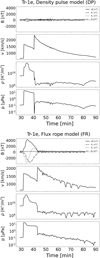 |
Fig. B.1 Profiles of all plasma quantities during the CME event (DP left, FR right) of our basic model (1031 erg) for Trappist-1e. The profiles are obtained in front of the planetary bow shock letting time evolve. |
Appendix C Influence of CME event duration on interior Joule heating
In the Solar System CME events typically last for several hours up to a few days. In order to assess the effect of event duration on the results of this work, we additionally performed simulations with CME event durations up to 3 hours.
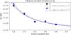 |
Fig. C.1 Interior heating rates as a function of CME event duration (hours). Circles depict DP and triangles FR results. Dashed lines show the fitted curves with the fitting parameters shown in the legend. |
We restricted the additional simulations to the DP CME scenario (1031 erg) with Bp = 0.05 G and event duration of 1 h, 1.5 h, 2 h, 2.5 h and 3 h. We extended the CME peak (DP model) in form of a plateau with maximum amplitude from the CME center toward the front in such a way so that the front of the curve (i.e., the nose of the Gaussian) has the same shape as in our basic model. With this setup the shape of the shock and sheath region of the CME remain the same. The tail of the CME is, however, stretched out accordingly to match the desired event duration. We find in our results that the heating rates for a single event decrease toward longer event durations (Fig. C). This is caused by the slower decay of the CME parameters in the tail and by the longer averaging period for dB/dt. The magnetosphere weakly pulsates during the sustain phase in which we extend the CME peak. This is caused by compression and repulsive expansion of the dayside magnetosphere, and thus the extended peak still leads to magnetic variability near the planet, although of small amplitude. We fit the heating rates as a function of event duration (dashed lines in Fig. C). Extrapolating QJ toward longer CME durations we find a saturation of interior heating at about half the value of our basic 1-hour CME model. We note that this result is likely a consequence of our CME model choices and we do not derive a general trend for CMEs from it but point out that, in our CME model, the event duration only weakly influences the results presented in this work.
Appendix D Poynting flux maps
Here we present maps of inward Poynting flux components  obtained at the planet’s surface (Fig. D.1) complementary to the discussion in Sect. 4.1, Fig. 12. The maps demonstrate the well spatial alignment of the Poynting fluxes with the time-averaged magnetic variability of the radial field component dB/dt (Fig. 10). The distribution of radial Poynting fluxes support our conclusion that magnetic variability is dominantly generated by magnetospheric compression due to the increased occurrence of
  within the closed magnetosphere (i.e., at low latitudes).
 |
Fig. D.1 Maps of inward, radial Poynting flux components, Sr, above the surface of Trappist-1e in the DP (top) and FR (bottom) scenario. Maps are shown during the CME sheath (left), peak (middle) and tail crossing (right) (see also Fig. 1). |
References
- Aarnio, A. N., Matt, S. P., & Stassun, K. G. 2012, ApJ, 760, 9 [NASA ADS] [CrossRef] [Google Scholar]
- Agol, E., Dorn, C., Grimm, S. L., et al. 2021, PSJ, 2, 1 [NASA ADS] [Google Scholar]
- Airapetian, V. S., Glocer, A., Khazanov, G. V., et al. 2017, ApJ, 836, L3 [NASA ADS] [CrossRef] [Google Scholar]
- Airapetian, V. S., Danchi, W. C., Dong, C. F., et al. 2018, arXiv e-prints, [arXiv:1801.07333] [Google Scholar]
- Airapetian, V. S., Barnes, R., Cohen, O., et al. 2020, Int. J. Astrobiol., 19, 136 [NASA ADS] [CrossRef] [Google Scholar]
- Alvarado-Gómez, J. D., Drake, J. J., Cohen, O., Moschou, S. P., & Garraffo, C. 2018, ApJ, 862, 93 [Google Scholar]
- Barr, A. C., Dobos, V., & Kiss, L. L. 2018, A&A, 613, A37 [NASA ADS] [CrossRef] [EDP Sciences] [Google Scholar]
- Baumjohann, W., & Treumann, R. A. 2012, Basic Space Plasma Physics (Imperial College Press) [Google Scholar]
- Birky, J., Barnes, R., & Fleming, D. P. 2021, RNAAS, 5, 122 [NASA ADS] [Google Scholar]
- Bolmont, E., Breton, S. N., Tobie, G., et al. 2020, A&A, 644, A165 [NASA ADS] [CrossRef] [EDP Sciences] [Google Scholar]
- Bourrier, V., de Wit, J., Bolmont, E., et al. 2017, AJ, 154, 121 [NASA ADS] [CrossRef] [Google Scholar]
- Chané, E., van der Holst, B., Jacobs, C., Poedts, S., & Kimpe, D. 2006, A&A, 447, 727 [NASA ADS] [CrossRef] [EDP Sciences] [Google Scholar]
- Chen, P. F. 2011, Living Rev. Sol. Phys., 8, 1 [Google Scholar]
- Chen, A. Q., Chen, P. F., & Fang, C. 2006, A&A, 456, 1153 [NASA ADS] [CrossRef] [EDP Sciences] [Google Scholar]
- Christensen, A. B., Yee, J.-H., Bishop, R. L., et al. 2012, JGR Space Phys., 117, A04315 [Google Scholar]
- Cohen, O., Glocer, A., Garraffo, C., et al. 2024, ApJ, 962, 157 [NASA ADS] [CrossRef] [Google Scholar]
- Compagnino, A., Romano, P., & Zuccarello, F. 2017, Sol. Phys., 292, 5 [Google Scholar]
- Dasso, S., Mandrini, C. H., Démoulin, P., & Luoni, M. L. 2006, A&A, 455, 349 [NASA ADS] [CrossRef] [EDP Sciences] [Google Scholar]
- Davies, A. G., Perry, J. E., Williams, D. A., & Nelson, D. M. 2024, Nat. Astron., 8, 94 [Google Scholar]
- de Wit, J., Wakeford, H. R., Lewis, N. K., et al. 2018, Nat. Astron., 2, 214 [NASA ADS] [CrossRef] [Google Scholar]
- Dedner, A., Kemm, F., Kröner, D., et al. 2002, JCP, 175, 645 [NASA ADS] [Google Scholar]
- Démoulin, P., Janvier, M., & Dasso, S. 2016, Sol. Phys., 291, 531 [Google Scholar]
- Desai, R. T., Zhang, H., Davies, E. E., et al. 2020, Sol. Phys., 295, 130 [NASA ADS] [CrossRef] [Google Scholar]
- Dobos, V., Barr, A. C., & Kiss, L. L. 2019, A&A, 624, A2 [NASA ADS] [CrossRef] [EDP Sciences] [Google Scholar]
- Dong, C., Jin, M., Lingam, M., et al. 2018, PNAS, 115, 260 [NASA ADS] [CrossRef] [Google Scholar]
- Ducrot, E., Gillon, M., Delrez, L., et al. 2020, A&A, 640, A112 [NASA ADS] [CrossRef] [EDP Sciences] [Google Scholar]
- Duling, S., Saur, J., & Wicht, J. 2014, JGR Space Phys., 119, 4412 [Google Scholar]
- Elekes, F., & Saur, J. 2023, A&A, 671, A133 [NASA ADS] [CrossRef] [EDP Sciences] [Google Scholar]
- Fleming, D. P., Barnes, R., Luger, R., & VanderPlas, J. T. 2020, ApJ, 891, 155 [NASA ADS] [CrossRef] [Google Scholar]
- García Muñoz, A. 2023, A&A, 672, A77 [NASA ADS] [CrossRef] [EDP Sciences] [Google Scholar]
- Garraffo, C., Drake, J. J., Cohen, O., Alvarado-Gómez, J. D., & Moschou, S. P. 2017, ApJ, 843, L33 [Google Scholar]
- Gillon, M., Triaud, A. H. M. J., Demory, B.-O., et al. 2017, Nature, 542, 456 [NASA ADS] [CrossRef] [Google Scholar]
- Glazier, A. L., Howard, W. S., Corbett, H., et al. 2020, ApJ, 900, 27 [Google Scholar]
- Godolt, M., Tosi, N., Stracke, B., et al. 2019, A&A, 625, A12 [NASA ADS] [CrossRef] [EDP Sciences] [Google Scholar]
- Gold, T., & Hoyle, F. 1960, MNRAS, 120, 89 [NASA ADS] [Google Scholar]
- Gopalswamy, N., Yashiro, S., & Akiyama, S. 2015, ApJ, 809, 106 [Google Scholar]
- Grayver, A., Bower, D. J., Saur, J., Dorn, C., & Morris, B. M. 2022, ApJ, 941, L7 [NASA ADS] [CrossRef] [Google Scholar]
- Greene, T. P., Bell, T. J., Ducrot, E., et al. 2023, Nature, 618, 39 [NASA ADS] [CrossRef] [Google Scholar]
- Günther, M. N., Zhan, Z., Seager, S., et al. 2020, AJ, 159, 60 [Google Scholar]
- Höning, D., & Spohn, T. 2023, Astrobiology, 23, 372 [Google Scholar]
- Höning, D., Tosi, N., & Spohn, T. 2019, A&A, 627, A48 [NASA ADS] [CrossRef] [EDP Sciences] [Google Scholar]
- Hosteaux, S., Chané, E., & Poedts, S. 2019, A&A, 632, A89 [NASA ADS] [CrossRef] [EDP Sciences] [Google Scholar]
- Howard, W. S., Kowalski, A. F., Flagg, L., et al. 2023, ApJ, 959, 64 [NASA ADS] [CrossRef] [Google Scholar]
- Ilin, E., Poppenhaeger, K., Schmidt, S. J., et al. 2021, MNRAS, 507, 1723 [CrossRef] [Google Scholar]
- Jian, L., Russell, C. T., Luhmann, J. G., & Skoug, R. M. 2006, Sol. Phys., 239, 393 [NASA ADS] [CrossRef] [Google Scholar]
- Johnstone, C. P., Güdel, M., Lammer, H., & Kislyakova, K. G. 2018, A&A, 617, A107 [NASA ADS] [CrossRef] [EDP Sciences] [Google Scholar]
- Kay, C., Airapetian, V. S., Lüftinger, T., & Kochukhov, O. 2019, ApJ, 886, L37 [NASA ADS] [CrossRef] [Google Scholar]
- Keiling, A. 2009, Space Sci. Rev., 142, 73 [Google Scholar]
- Kislyakova, K., & Noack, L. 2020, A&A, 636, L10 [NASA ADS] [CrossRef] [EDP Sciences] [Google Scholar]
- Kislyakova, K. G., Noack, L., Johnstone, C. P., et al. 2017, Nat. Astron., 1, 878 [NASA ADS] [CrossRef] [Google Scholar]
- Kislyakova, K. G., Fossati, L., Johnstone, C. P., et al. 2018, ApJ, 858, 105 [NASA ADS] [CrossRef] [Google Scholar]
- Krishnamurthy, V., Hirano, T., Stefánsson, G., et al. 2021, AJ, 162, 82 [CrossRef] [Google Scholar]
- Krissansen-Totton, J. 2023, ApJ, 951, L39 [NASA ADS] [CrossRef] [Google Scholar]
- Krissansen-Totton, J., & Fortney, J. J. 2022, ApJ, 933, 115 [NASA ADS] [CrossRef] [Google Scholar]
- Krissansen-Totton, J., Wogan, N., Thompson, M., & Fortney, J. J. 2024, Nat. Commun., 15, 8374 [Google Scholar]
- Lin, J., Wang, F., Deng, L., et al. 2022, ApJ, 932, 62 [Google Scholar]
- Lincowski, A. P., Meadows, V. S., Zieba, S., et al. 2023, ApJ, 955, L7 [NASA ADS] [CrossRef] [Google Scholar]
- Luger, R., Sestovic, M., Kruse, E., et al. 2017, Nat. Astron., 1, 0129 [Google Scholar]
- Mignone, A., Bodo, G., Massaglia, S., et al. 2007, in JENAM-2007, “Our Non Stable Universe”, 96 [Google Scholar]
- Mignone, A., Tzeferacos, P., & Bodo, G. 2010, JCP, 229, 5896 [Google Scholar]
- Moschou, S.-P., Drake, J. J., Cohen, O., et al. 2019, ApJ, 877, 105 [NASA ADS] [CrossRef] [Google Scholar]
- Naif, S., Selway, K., Murphy, B. S., Egbert, G., & Pommier, A. 2021, Phys. Earth Planet. Inter., 313, 106661 [Google Scholar]
- Park, J., Lühr, H., Knudsen, D. J., Burchill, J. K., & Kwak, Y.-S. 2017, JGR Space Phys., 122, 2345 [Google Scholar]
- Patsourakos, S., & Georgoulis, M. K. 2017, Sol. Phys., 292, 89 [NASA ADS] [CrossRef] [Google Scholar]
- Paudel, R. R., Gizis, J. E., Mullan, D. J., et al. 2018, ApJ, 858, 55 [Google Scholar]
- Payne, R. C., & Kaltenegger, L. 2024, MNRAS, 530, L13 [NASA ADS] [CrossRef] [Google Scholar]
- Peale, S. J., Cassen, P., & Reynolds, R. T. 1979, Science, 203, 892 [Google Scholar]
- Roettenbacher, R. M., & Kane, S. R. 2017, ApJ, 851, 77 [Google Scholar]
- Saur, J., Grambusch, T., Duling, S., Neubauer, F. M., & Simon, S. 2013, A&A, 552, A119 [NASA ADS] [CrossRef] [EDP Sciences] [Google Scholar]
- Saur, J., Janser, S., Schreiner, A., et al. 2018, JGR Space Phys., 123, 9560 [Google Scholar]
- Saur, J., Willmes, C., Fischer, C., et al. 2021, A&A, 655, A75 [NASA ADS] [CrossRef] [EDP Sciences] [Google Scholar]
- Scolini, C., Dasso, S., Rodriguez, L., Zhukov, A. N., & Poedts, S. 2021, A&A, 649, A69 [NASA ADS] [CrossRef] [EDP Sciences] [Google Scholar]
- Seli, B., Vida, K., Moór, A., Pál, A., & Oláh, K. 2021, A&A, 650, A138 [NASA ADS] [CrossRef] [EDP Sciences] [Google Scholar]
- Shibata, K., & Magara, T. 2011, Living Rev. Sol. Phys., 8, 6 [NASA ADS] [Google Scholar]
- Song, H. Q., Zhang, J., Cheng, X., et al. 2020, ApJ, 901, L21 [NASA ADS] [CrossRef] [Google Scholar]
- Strack, D., & Saur, J. 2024, JGR Space Phys., 129, 2024JA033235 [Google Scholar]
- Strickert, K. M., Evensberget, D., & Vidotto, A. A. 2024, MNRAS, 533, 1156 [Google Scholar]
- Strugarek, A., García Muñoz, A., Brun, A. S., & Paul, A. 2025, A&A, 693, A220 [NASA ADS] [CrossRef] [EDP Sciences] [Google Scholar]
- Tilley, M. A., Segura, A., Meadows, V., Hawley, S., & Davenport, J. 2019, Astrobiology, 19, 64 [Google Scholar]
- Tosi, N., Godolt, M., Stracke, B., et al. 2017, A&A, 605, A71 [NASA ADS] [CrossRef] [EDP Sciences] [Google Scholar]
- Turbet, M., Bolmont, E., Ehrenreich, D., et al. 2020, A&A, 638, A41 [NASA ADS] [CrossRef] [EDP Sciences] [Google Scholar]
- Turner, J. D., Zarka, P., Grießmeier, J.-M., et al. 2021, A&A, 645, A59 [NASA ADS] [CrossRef] [EDP Sciences] [Google Scholar]
- Tyler, R. H., Henning, W. G., & Hamilton, C. W. 2015, ApJS, 218, 22 [Google Scholar]
- Tziotziou, K., Georgoulis, M. K., & Raouafi, N.-E. 2012, ApJ, 759, L4 [NASA ADS] [CrossRef] [Google Scholar]
- Unterborn, C. T., Foley, B. J., Desch, S. J., et al. 2022, ApJ, 930, L6 [NASA ADS] [CrossRef] [Google Scholar]
- Van Looveren, G., Güdel, M., Boro Saikia, S., & Kislyakova, K. 2024, A&A, 683, A153 [Google Scholar]
- Vasyliu¯nas, V. M., & Song, P. 2005, JGR Space Phys., 110, A02301 [Google Scholar]
- Veronig, A. M., Odert, P., Leitzinger, M., et al. 2021, Nat. Astron., 5, 697 [NASA ADS] [CrossRef] [Google Scholar]
- Vida, K., Ko˝vári, Z., Pál, A., Oláh, K., & Kriskovics, L. 2017, ApJ, 841, 124 [NASA ADS] [CrossRef] [Google Scholar]
- Walls, F. L., & Dunn, G. H. 1974, J. Geophys. Res., 79, 1911 [Google Scholar]
- Wang, Y., Zhuang, B., Hu, Q., et al. 2016, JGR Space Phys., 121, 9316 [Google Scholar]
- Wheatley, P. J., Louden, T., Bourrier, V., Ehrenreich, D., & Gillon, M. 2017, MNRAS, 465, L74 [NASA ADS] [CrossRef] [Google Scholar]
- Wilson, D. J., Froning, C. S., Duvvuri, G. M., et al. 2021, ApJ, 911, 18 [NASA ADS] [CrossRef] [Google Scholar]
- Yang, Z., Zhang, L., Meng, G., et al. 2023, A&A, 669, A15 [NASA ADS] [CrossRef] [EDP Sciences] [Google Scholar]
- Yashiro, S., & Gopalswamy, N. 2009, in IAU Symposium, 257, Universal Heliophysical Processes, eds. N. Gopalswamy & D. F. Webb, 233 [Google Scholar]
- Youssef, M. 2012, NRJAG, 1, 172 [Google Scholar]
- Zieba, S., Kreidberg, L., Ducrot, E., et al. 2023, Nature, 620, 746 [NASA ADS] [CrossRef] [Google Scholar]
All Tables
Time-averaged annual Joule heating rates (TW) in the interior of Trappist-1b and e due to CMEs.
All Figures
|
Fig. 1 Basic structure of the modeled CMEs. The values are extracted from a fixed location in front of the bow shock. |
| In the text | |
|
Fig. 2 Density pulse model results. The xz-plane cross sections are centered at Trappist-1e (see Sect. 2). Positions are given in planetary radii. Arrows depict velocity vectors and their colors velocity magnitudes (left color bar). Contours indicate plasma density (right color bar). Black and magenta lines indicate interplanetary and planetary magnetic field lines projected onto the xz-plane, respectively. We display the cross sections before the CME shock (top), during the shock crossing (upper middle), during the shath (bottom middle) and during the CME peak (bottom). Each column is for a specified intrinsic magnetic field strength, Bp. |
| In the text | |
|
Fig. 3 Same as Fig. 2 but for the for the FR model. Because of a slightly enhanced CME size due to the FR magnetic pressure the CME shock crossing occurs approximately 30 s later compared to the DP case. |
| In the text | |
|
Fig. 4 Upstream magnetopause locations (in planetary radii Rp) of Trappist-1e for a planetary field with surface strength Bp = 0.03, 0.05, 0.15, and 0.21 G as a function of time. The upper and bottom panels display the DP and FR model runs, respectively. |
| In the text | |
|
Fig. 5 Schematic of the post-processing pipeline to calculate the CME-induced Joule heating in the interior of a planet. |
| In the text | |
|
Fig. 6 Evolution of the external Gauss coefficients (Eq. (18)) during one CME as a function of time (minutes) for planetary magnetic field strength: Bp = 0 (top), 0.03 (upper middle), 0.07 (lower middle), and 0.21 G (bottom). The left column shows DP; the right column shows FR model results. Displayed are all considered external Gauss coefficients ( |
| In the text | |
|
Fig. 7 Joule heating averaged within 1-hour CME events in the interior of the planets, QJ (Eq. (17)), given in Watts as a function of planetary magnetic field strength, Bp. Triangles denote FR, circles DP CME cases. Yellow data points correspond to Trappist-1e, purple to Trappist-1e. Green data points denote the results with an atmosphere around Trappist-1e. |
| In the text | |
|
Fig. 8 Heating rates at Bp = 0.11 G for Trappist-1e as a function of the electric conductivity, σ, in S/m. The brown vertical line indicates the homogeneous model conductivity adopted in this study. |
| In the text | |
|
Fig. 9 Ionospheric Joule heating rates (Eq. (20)) averaged within 1 hour CME events for Trappist-1e as a function of planetary magnetic field Bp. The DP and FR model results are denoted by circles and triangles, respectively. The dayside XUV power received from the star is also indicated. |
| In the text | |
|
Fig. 10 Maps of time-averaged magnetic variability, dB/dt (nT/s), of the radial magnetic field component obtained directly above the planetary surface. Co-latitude and longitude are shown on the Y and X axes, respectively. Upstream direction is at longitude below 180 degrees. Model results are shown in the left column for the DP and in the right column for the FR case. We show maps for Bp = 0 (top), 0.05 (middle) and 0.15 G (bottom). |
| In the text | |
|
Fig. 11 Sketch illustrating the generation of the background magnetic field aligned Poynting fluxes associated with Alfvén waves. We do not show fast mode waves due to the negligible effect on the radial components of near-surface magnetic variability, dB/dt, found with our model. |
| In the text | |
|
Fig. 12 Open-closed field line boundary (red lines) plotted on top of an inward Poynting flux, Sin, map for Trappist-1e, Bp = 0.21 G, DP model. As an example, the map is shown during the CME sheath crossing, but the boundary remains almost constant over the entire simulation period for DP as well as FR simulations. |
| In the text | |
|
Fig. 13 Time series of |
| In the text | |
|
Fig. 14 Time-averaged inward Poynting fluxes |
| In the text | |
|
Fig. 15 Time-averaged interior heating rates as a function of CME-associated flare energy Eflare (erg) for DP (a) and FR (b) CMEs. We only show heating rates for Bp = 0 G (black circles), Bp = 0.05 G (blue upward triangles), Bp = 0.11 G (green downward triangles), and Bp = 0.17 G (yellow diamonds). Gray triangles denote the incident total energy flux of the CME (right y-axis). |
| In the text | |
|
Fig. B.1 Profiles of all plasma quantities during the CME event (DP left, FR right) of our basic model (1031 erg) for Trappist-1e. The profiles are obtained in front of the planetary bow shock letting time evolve. |
| In the text | |
|
Fig. C.1 Interior heating rates as a function of CME event duration (hours). Circles depict DP and triangles FR results. Dashed lines show the fitted curves with the fitting parameters shown in the legend. |
| In the text | |
|
Fig. D.1 Maps of inward, radial Poynting flux components, Sr, above the surface of Trappist-1e in the DP (top) and FR (bottom) scenario. Maps are shown during the CME sheath (left), peak (middle) and tail crossing (right) (see also Fig. 1). |
| In the text | |
Current usage metrics show cumulative count of Article Views (full-text article views including HTML views, PDF and ePub downloads, according to the available data) and Abstracts Views on Vision4Press platform.
Data correspond to usage on the plateform after 2015. The current usage metrics is available 48-96 hours after online publication and is updated daily on week days.
Initial download of the metrics may take a while.