| Issue |
A&A
Volume 700, August 2025
|
|
|---|---|---|
| Article Number | A156 | |
| Number of page(s) | 37 | |
| Section | Stellar structure and evolution | |
| DOI | https://doi.org/10.1051/0004-6361/202554768 | |
| Published online | 22 August 2025 | |
Massive stars exploding in a He-rich circumstellar medium
XI. Diverse evolution of five Ibn SNe 2020nxt, 2020taz, 2021bbv, 2023utc, and 2024aej
1
School of Physics and Astronomy, Beijing Normal University, Beijing 100875, China
2
Department of Physics, Faculty of Arts and Sciences, Beijing Normal University, Zhuhai 519087, China
3
INAF – Osservatorio Astronomico di Padova, Vicolo dell’Osservatorio 5, 35122 Padova, Italy
4
Yunnan Observatories, Chinese Academy of Sciences, Kunming 650216, China
5
International Centre of Supernovae, Yunnan Key Laboratory, Kunming 650216, China
6
Key Laboratory for the Structure and Evolution of Celestial Objects, Chinese Academy of Sciences, Kunming 650216, China
7
School of Physics, O’Brien Centre for Science North, University College Dublin, Belfield, Dublin 4, Ireland
8
INAF – Osservatorio Astronomico di Brera, Via E. Bianchi 46, 23807 Merate (LC), Italy
9
Department of Astronomy, Xiamen University, Xiamen, Fujian 361005, China
10
Department of Physics, Tsinghua University, Beijing 100084, China
11
INAF – Osservatorio Astronomico d’Abruzzo, Via M. Maggini snc, 64100 Teramo, Italy
12
Las Cumbres Observatory, 6740 Cortona Drive, Suite 102, Goleta, CA 93117-5575, USA
13
Department of Physics, University of California, Santa Barbara, CA 93106-9530, USA
14
Institute of Space Sciences (ICE, CSIC), Campus UAB, Carrer de Can Magrans, s/n, E-08193 Barcelona, Spain
15
Institut für Theoretische Physik, Goethe Universität, Max-von-Laue-Str. 1, 60438 Frankfurt am Main, Germany
16
Center for Astrophysics | Harvard & Smithsonian, 60 Garden Street, Cambridge, MA 02138-1516, USA
17
The NSF AI Institute for Artificial Intelligence and Fundamental Interactions, USA
18
Tuorla Observatory, Department of Physics and Astronomy, University of Turku, FI-20014 Turku, Finland
19
Key Laboratory of Optical Astronomy, National Astronomical Observatories, Chinese Academy of Sciences, Beijing 100101, China
20
The Oskar Klein Centre, Department of Astronomy, Stockholm University, AlbaNova, SE-10691 Stockholm, Sweden
21
Astrophysics Research Institute, Liverpool John Moores University, IC2, Liverpool Science Park, 146 Brownlow Hill, Liverpool L3 5RF, UK
22
Max-Planck-Institut für Astrophysik, Karl-Schwarzschild Str. 1, D-85748 Garching, Germany
23
School of Physics and Astronomy, University of Leicester, University Road, Leicester LE1 7RH, UK
24
College of Science, Chongqing University of Posts and Telecommunications, Chongqing 400065, China
25
Astrophysics Research Centre, School of Mathematics and Physics, Queen’s University Belfast BT7 1NN, UK
26
Astrophysics sub-Department, Department of Physics, University of Oxford, Keble Road, Oxford OX1 3RH, UK
27
Department of Physics and Astronomy, Aarhus University, Ny Munkegade 120, DK-8000 Aarhus C, Denmark
28
Adler Planetarium, 1300 S. DuSable Lake Shore Drive, Chicago, IL 60605, USA
29
Department of Physics, Stellenbosch University, Matieland 7602, South Africa
30
National Institute for Theoretical and Computational Sciences (NITheCS), South Africa
31
Purple Mountain Observatory, Chinese Academy of Sciences, Nanjing 210023, China
32
Institute for Astronomy, University of Hawai’i, 2680 Woodlawn Drive, Honolulu HI, 96822, USA
33
Institut d’Estudis Espacials de Catalunya (IEEC), 08860 Castelldefels (Barcelona), Spain
34
Finnish Centre for Astronomy with ESO (FINCA), Quantum, Vesilinnantie 5, University of Turku, FI-20014 Turku, Finland
35
School of Physics and Electrical Engineering, Liupanshui Normal University, Liupanshui, Guizhou 553004, China
36
Cosmic Dawn Center (DAWN), Denmark
37
Niels Bohr Institute, University of Copenhagen, Jagtvej 128, 2200 København N, Denmark
38
School of Physics and Electronic Information, Jiangsu Second Normal University, Nanjing, Jiangsu 211200, China
39
Institute for Frontier in Astronomy and Astrophysics, Beijing Normal University, Beijing 102206, China
40
Advanced Institute of Natural Sciences, Beijing Normal University, Zhuhai 519087, China
⋆ Corresponding authors: This email address is being protected from spambots. You need JavaScript enabled to view it.
; This email address is being protected from spambots. You need JavaScript enabled to view it.
; This email address is being protected from spambots. You need JavaScript enabled to view it.
Received:
26
March
2025
Accepted:
16
June
2025
Abstract
We present the photometric and spectroscopic analysis of five Type Ibn supernovae (SNe): SN 2020nxt, SN 2020taz, SN 2021bbv, SN 2023utc, and SN 2024aej. These events share key observational features and belong to a family of objects similar to the prototypical Type Ibn SN 2006jc. The SNe exhibit rise times of approximately 10 days and peak absolute magnitudes ranging from −16.5 to −19 mag. Notably, SN 2023utc is the faintest Type Ibn SN discovered to date, with an exceptionally low r-band absolute magnitude of −16.4 mag. The pseudo-bolometric light curves peak at (1 − 10)×1042 erg s−1, with total radiated energies on the order of (1 − 10)×1048 erg. Spectroscopically, these SNe display a relatively slow spectral evolution. The early spectra are characterised by a hot blue continuum and prominent He I emission lines. The early spectra also show blackbody temperatures exceeding 10 000 K, with a subsequent decline in temperature during later phases. Narrow He I lines, which are indicative of unshocked circumstellar material (CSM), show velocities of approximately 1000 km s−1. The spectra suggest that the progenitors of these SNe underwent significant mass loss prior to the explosion, resulting in a He-rich CSM. Our light curve modelling yielded estimates for the ejecta mass (Mej) in the range 1 − 3 M⊙ with kinetic energies (EKin) of (0.1 − 1)×1050 erg. The inferred CSM mass ranges from 0.2 to 1 M⊙. These findings are consistent with expectations for core collapse events arising from relatively massive envelope-stripped progenitors.
Key words: circumstellar matter / supernovae: individual: SN 2020nxt / supernovae: individual: SN 2020taz / supernovae: individual: SN 2021bbv / supernovae: individual: SN 2023utc / supernovae: individual: SN 2024aej
© The Authors 2025
 Open Access article, published by EDP Sciences, under the terms of the Creative Commons Attribution License (https://creativecommons.org/licenses/by/4.0), which permits unrestricted use, distribution, and reproduction in any medium, provided the original work is properly cited.
This article is published in open access under the Subscribe to Open model. This email address is being protected from spambots. You need JavaScript enabled to view it. to support open access publication.
1. Introduction
Type Ibn supernovae (SNe Ibn) are a subclass of stellar explosions characterised by narrow (∼1000 km s−1) helium emission lines in their spectra, which indicate the presence of He-rich circumstellar material (CSM; Smith 2017; Gal-Yam 2017). The first discovered Type Ibn SN, SN 1999cq, was found by Matheson et al. (2000), but the formal designation of the new SN type was introduced later by Pastorello et al. (2008a) after publication of the first studies on SN 2006jc, the prototypical SN of this class (e.g. Foley et al. 2007; Pastorello et al. 2007; Anupama et al. 2009).
SNe Ibn are rare, with only 73 confirmed events to date1. Maeda & Moriya (2022) estimated their volumetric rate to be ∼1% of all core-collapse supernovae (CC SNe), while Perley et al. (2020) reported a detection rate of 0.66% within the Zwicky Transient Facility (ZTF) transient sample. Furthermore, Ma et al. (2025a,b) analysed a nearby SN sample within 40 Mpc – compiled primarily from wide-field surveys conducted between 2016 and 2023 – and found that SNe Ibn comprise around 1% of the total sample. Despite significant progress in the discovery and characterisation of SNe Ibn, their progenitor systems remain enigmatic due to the limited sample size and the diversity in their observed properties (Maund et al. 2016; Maeda & Moriya 2022; Dessart et al. 2022).
Hosseinzadeh et al. (2017) suggest that SNe Ibn exhibit an overall photometric homogeneity but show significant spectral diversity around the maximum light. From a spectroscopic point of view, SNe Ibn are characterised by narrow He I emission lines with full width at half maximum (FWHM) velocities ranging from a hundred to a few thousand km s−1 (Pastorello et al. 2016; Hosseinzadeh et al. 2017). In some cases, weak hydrogen lines have also been detected in the spectra, suggesting the presence of a residual amount of H in the CSM (Pastorello et al. 2008b, 2015a; Smith et al. 2012; Reguitti et al. 2022; Wang et al. 2024a). SNe Ibn light curves usually exhibit fast rise times (≤15 days), rapid post-peak declines (0.05–0.15 mag day−1), and a peak absolute magnitude of M ∼ −19 mag.
Despite the findings of photometric homogeneity (Hosseinzadeh et al. 2017), there are a few outliers, including the superluminous SN ASASSN-14ms (MV ∼ − 20.5 mag; Vallely et al. 2018; Wang et al. 2021a), long-lasting transients such as OGLE2012-SN-006 (Pastorello et al. 2015b), the double-peaked iPTF13beo (Gorbikov et al. 2014), and the slow-rising OGLE-2014-SN-131 (Karamehmetoglu et al. 2017). This diversity could be due to a variety of progenitor systems and explosion mechanisms for SNe Ibn, although in most cases they are considered stripped-envelope CC SNe interacting with He-rich environments (Chugai 2009)2.
The progenitor systems of SNe Ibn are an area of active investigation, with multiple channels proposed to explain their diverse observational characteristics. Initially, the progenitors were identified as massive (MZAMS ≥ 25 M⊙) hydrogen-poor Wolf-Rayet (WR) stars embedded in a He-rich CSM (Pastorello et al. 2007). These WR stars undergo substantial mass loss prior to core collapse that results in the formation of a dense CSM. When the fast-moving SN ejecta collide with the slow CSM, shocks are generated that heat and ionise the He-rich material in the CSM, leading to the formation of the narrow He emission lines characteristic of SNe Ibn. The frequent association of SNe Ibn with active star-forming regions supports this scenario (Taddia et al. 2015; Pastorello et al. 2015a). However, the Type Ibn SN PS1-12sk occurred in the outskirts of an elliptical galaxy with low star formation activity, challenging the massive star progenitor scenario as the sole channel producing SNe Ibn (Sanders et al. 2013).
An alternative progenitor scenario involves lower-mass (final masses ≲5 M⊙; Dessart et al. 2022) helium stars in binary systems, where binary interaction drives episodic mass losses gathering the CSM prior to the core collapse (Maund et al. 2016). Late-time Hubble Space Telescope (HST) images of SNe Ibn explosion sites indicate that at least some SNe Ibn were in relatively low-mass binary systems (Sun et al. 2020). Binary systems may account for SNe Ibn in older stellar populations, with Dessart et al. (2022) providing evidence for low-mass binary progenitors through spectral modelling. Furthermore, some Type IIb SNe, which explode within dense He-rich CSM and evolve into SNe Ibn features, suggest that multiple progenitor pathways might lead to Type Ibn SN (Prentice et al. 2020). Thus, while SNe Ibn are unified by their spectroscopic signatures, their progenitor systems likely encompass a range of evolutionary scenarios, reflecting both single and binary star channels. Metzger (2022) proposed a novel mechanism for SNe Ibn, suggesting that their emission could be powered by disc outflows resulting from hyper-accretion onto a compact object, such as a neutron star or black hole, located in the vicinity of a helium star, rather than being driven by stellar mass loss. This mechanism also predicts a relatively low yield of 56Ni.
X-ray observations, though only occasionally employed, provide a direct means of probing the mass-loss history of the SN progenitor. The X-ray emission is produced by forward and reverse shocks arising from the ejecta-CSM interaction (Chevalier & Fransson 1994), and it allows the density of the CSM and the mass distribution to be constrained, thus enabling estimates of progenitor mass-loss rates in the last years before the explosion (e.g. Immler et al. 2001; Tsuna et al. 2021; Margalit et al. 2022). To our knowledge, only two SNe Ibn, SN 2006jc (Immler et al. 2008) and SN 2022ablq (Pellegrino et al. 2024), have well-sampled X-ray light curves. In SN 2006jc, the X-ray flux peaked at ∼100 days after the explosion and was attributed to the shock encountering a dense shell ejected two years earlier, consistent with a previously observed optical outburst (Immler et al. 2008). The inferred CSM mass exceeded 0.01 M⊙. For SN 2022ablq, enhanced mass-loss rates ranging from 0.05 to 0.5 M⊙ yr−1 were noticed from 2 to 0.5 years before the explosion, suggesting an eruptive event from a lower-mass progenitor rather than steady winds from a WR star (Pellegrino et al. 2024). More recently, Inoue & Maeda (2025) developed broadband X-ray light-curve models for SNe Ibn/Icn that have provided theoretical predictions to guide future high-cadence X-ray observations of interacting transients.
In this paper, we present a detailed analysis of the photometric and spectroscopic observations of five SNe Ibn, SNe 2020nxt, 2020taz, 2021bbv, 2023utc, and 2024aej, in order to investigate their observational properties and compare them with previously studied events. The basic discovery details, including distance and extinction estimates, are outlined in Section 2. In Section 3, we examine their light curves and fit light curve models to derive key physical parameters. A comprehensive analysis of the spectral properties of these SNe Ibn is presented in Section 4. Finally, we discuss and summarise our findings in Section 5.
2. Basic sample information
2.1. Individual objects
2.1.1. SN 2020nxt
SN 2020nxt (also known with the survey designations ATLAS20rzv and PS20geh) was first detected by the Asteroid Terrestrial-impact Last Alert System (ATLAS, equipped with the ACAM1 camera mounted on the ATLAS Haleakala Telescope; Tonry et al. 2018; Smith et al. 2020; Shingles et al. 2021), on 03.54 July 2020 UT (MJD = 59033.54; UT dates are used throughout the article) at the orange filter magnitude of o = 17.19 mag (AB, Tonry et al. 2020). The last ATLAS non-detection was on 30.56 June 2020 (MJD = 59030.56) in the o band, with an estimated upper limit of 20.76 mag3. The spectrum of this transient showed a match with the Type Ibn SN 2006jc, about 10 days past explosion. This supported the classification of SN 2020nxt as a Type Ibn SN (Srivastav et al. 2020). SN 2020nxt, at RA =  , Dec =
  (all coordinates in this paper are given in J2000), is possibly associated with a galaxy named SDSS J223736.60+350007.4 (2MASXJ22373660+3500074), with the SN being 1
 15 north and 5
 76 west from the galaxy centre (see Fig. 1).
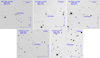 |
Fig. 1. SN 2020nxt in a NOT/ALFOSC image taken with a Sloan i-band filter on 19 July 2020; SN 2020taz in a NOT/ALFOSC image taken with a Sloan r-band filter on 1 October 2020; SN 2021bbv in a NOT/ALFOSC image taken with a Sloan i-band filter on 17 February 2021; SN 2023utc in a LCO TFN/fa20 image taken with a Sloan i-band filter on 27 October 2023; SN 2024aej in a LCO TFN/fa11 image taken with a Sloan r-band filter on 17 January 2024. |
We adopted the redshift of the host galaxy, z = 0.0218 ± 0.0003, from Wang et al. (2024b). Assuming a standard cosmology with H0 = 73 km s−1 Mpc−1, ΩM = 0.27, ΩΛ = 0.73 (used consistently throughout this paper; Spergel et al. 2007), we estimated a luminosity distance dL = 91.1 ± 1.2 Mpc (μ = 34.80 ± 0.03 mag)4 for SN 2020nxt. The Milky Way extinction in the SN direction is E(B − V)MW = 0.067 mag (Schlafly & Finkbeiner 2011).
2.1.2. SN 2020taz
The discovery of SN 2020taz (also known as ATLAS20baee, PS20hil, and ZTF20abyznqs) was announced by the Panoramic Survey Telescope and Rapid Response System (Pan-STARRS; Wainscoat et al. 2016) on 11.32 September 2020 (MJD = 59103.32) with a PanSTARRS-w filter brightness of 19.02 mag (AB, Chambers et al. 2020). A prediscovery detection was obtained by the ATLAS survey on 08.44 September 2020 (MJD = 59100.44), with the object having an o-band magnitude of o = 20.54 ± 0.24 mag5. The last non-detection, by the ZTF survey (Bellm et al. 2019), was on 07.33 September 2020 (MJD = 59099.33) in the r band, with an estimated limit of 20.13 mag6. Soon after the discovery, SN 2020taz was classified as a Type Ibn SN (Graham et al. 2020). Its coordinates are RA =  , Dec =
  .
.
SN 2020taz is located 3 60 west and 7
 74 south of the centre of its predicted host galaxy, WISEA J222606.51+103337.3 (PGC 1381253). The location of SN 2020taz is shown in Fig. 1. Adopting the recessional velocity of v = 14796 ± 140 km s−1 (hence a redshift z = 0.0494 ± 0.0005; Mould et al. 2000), and adopting the same standard cosmological model, we obtained a luminosity distance of dL = 210.7 ± 2.3 Mpc and hence a distance modulus of μL = 36.62 ± 0.02 mag. The Milky Way extinction is E(B − V)MW= 0.091 mag in this direction (Schlafly & Finkbeiner 2011).
Given the total apparent magnitude of PGC 1381253, as provided by HyperLeda7 (B = 17.04 ± 0.50), we derived a total absolute B-band magnitude of −20.17, after correction for Galactic extinction. Using the luminosity-metallicity relation from Tremonti et al. (2004), we estimated the overall oxygen abundance of PGC 1381253 to be 12 + log(O/H)=8.99 dex. Based on the radial metallicity gradient model by Pilyugin et al. (2004), we estimated the oxygen abundance at the SN site to be 12 + log(O/H)SN = 8.67 dex. This value is slightly above the mean oxygen abundances reported at the SN location for SNe Ibn host galaxies, such as 8.63 ± 0.42 dex by Pastorello et al. (2015c) and 8.45 ± 0.10 dex by Taddia et al. (2015).
2.1.3. SN 2021bbv
The discovery of SN 2021bbv (Gaia21akw, ZTF21aagyidr, PS21afl), attributed to the Gaia Photometric Science Alerts8, is dated 24.00 January 2021 (MJD = 59238.00). The object was observed in a Gaia-G filter image, with a magnitude of 18.7 mag (Hodgkin et al. 2021). However, an earlier detection was reported by the ZTF on 20.45 January 2021 (MJD = 59234.45), at a magnitude of g = 20.45 ± 0.33 mag9. The last non-detection provided by ATLAS was on 18.52 January 2021 (MJD = 59232.52) in the cyan (c) band, to a limit of 20.53 mag10. Soon after its discovery, the SN was classified as a Type Ibn event (Gonzalez et al. 2021). The SN coordinates are RA =  , Dec =
  (see Fig. 1).
SN 2021bbv is located 0.55 west and 0.36
 south of the centre of its predicted host galaxy, SDSS J113020.86+085535.0. Due to the lack of distance information, we inferred the kinematic distance of the host galaxy from measuring the central wavelength of the most prominent narrow He I (λ0 = 5875.6 Å) line in the SN spectra, and we obtained a redshift of z = 0.068 ± 0.003. Then, we obtained a luminosity distance of dL = 294.1 ± 13.6 Mpc and hence a distance modulus of μL = 37.34 ± 0.10 mag. The Milky Way extinction towards SN 2021bbv is E(B − V)MW= 0.033 mag (Schlafly & Finkbeiner 2011).
2.1.4. SN 2023utc
SN 2023utc (KATS23T003, ATLAS23ukm, ZTF23abjjrwv, PS23lcq) was discovered by the Xingming Sky Survey11 project on 11.94 October 2023 (corresponding to MJD = 60228.94). The object was observed in an unfiltered image with magnitude of 18.15 ± 0.21 (Zhang et al. 2023). The last ZTF non-detection in the g band was on 07.45 October 2023 (MJD = 60224.45), to a limit of 19.84 mag. Soon after discovery, the SN was classified as a Type Ibn event by Taguchi et al. (2023). The SN coordinates are RA =  , Dec =
  (see Fig. 1).
SN 2023utc is possibly associated with the host galaxy SDSS J091159.16+534304.2. Missing alternative distance estimates, and due to the lack of host galaxy lines in the spectra (see Section 4), we measured the central wavelength of the narrow He I SN lines and obtained a redshift of z = 0.014 ± 0.003. Then, we inferred a Hubble flow distance of dH = 57.5 ± 12.3 Mpc and hence a distance modulus of μH = 33.80 ± 0.46 mag. The Milky Way extinction towards this direction is E(B − V)MW= 0.015 mag (Schlafly & Finkbeiner 2011).
Given the apparent magnitude of SDSS J091159.16+534304.2 (g = 20.86 ± 0.05) as reported by SDSS12, we derived an absolute g-band magnitude of −13.00, after correcting for Galactic extinction. This places it among the faintest host galaxies for CC SNe (Li et al. 2011). Using the luminosity-metallicity relation from Tremonti et al. (2004), we estimated the overall oxygen abundance of SDSS J091159.16+534304.2 to be 12 + log(O/H)=7.613 dex, which is subsolar (adopting a solar metallicity of 12 + log(O/H)=8.69 dex; see e.g. von Steiger & Zurbuchen 2016; Vagnozzi 2019; Asplund et al. 2021), and lower than most SNe Ibn host galaxies (Taddia et al. 2015; Pastorello et al. 2015c). Due to the lack of detailed information on the host galaxy, we are unable to accurately estimate the oxygen abundance at the SN location.
2.1.5. SN 2024aej
The ATLAS discovery of SN 2024aej (ATLAS24awb, ZTF24aabwvws) is dated 14.32 January 2024 (MJD =60323.32), at an o-band brightness of 19.10 ± 0.14 mag (Tonry et al. 2024). However, an earlier detection was reported by ZTF on 14.22 January 2024 (MJD = 60323.22), at a magnitude of g = 18.85 ± 0.13 mag13. The last ATLAS non-detection in the o band is dated 11.32 January 2024 (MJD = 60320.32), to a limiting magnitude of 20.81 mag. Soon after its discovery, the SN was classified as a Type Ibn event by the Global Supernova Project (Terreran et al. 2024). The SN coordinates are RA =  , Dec =
  (see Fig. 1).
SN 2024aej is associated with a galaxy named WISEA J014427.03+390545.2. Due to the lack of alternative distance estimates, as for SN 2023utc, we measured the central wavelength of the narrow He I SN lines, and obtained a redshift of z = 0.063 ± 0.003. Then, we inferred a luminosity distance of dL = 271.5 ± 13.5 Mpc and hence a distance modulus of μL = 37.17 ± 0.11 mag. The Milky Way extinction in the SN direction is E(B − V)MW= 0.055 mag (Schlafly & Finkbeiner 2011).
2.2. Interstellar reddening
The information for the host galaxies of the five SNe Ibn in our sample is summarised in Table 1. Usually, dust extinction within the SN host galaxies can be inferred through empirical relations between the equivalent width (EW) of the narrow Na I doublet (Na I D) absorption line at the galaxy redshift, as observed in the early-time SN spectra, and the colour excess (see e.g. Turatto et al. 2003; Poznanski et al. 2012). Unfortunately, for our SN sample, the host galaxy extinction cannot be firmly constrained as a consequence of the modest S/N and limited spectral resolution of our spectra (see Sect. 4).
Basic information for the five Ibn SN host galaxies.
We closely examined the Na I D region in all available spectra (see Fig. A.1 in Appendix A), but the S/N of the spectra is insufficient to identify or place meaningful limits on the presence of host-galaxy Na I D absorption. In many cases, this spectral region is blended with He I λ5876 emission, and any potential Na I D absorption is indistinguishable from noise patterns. Consequently, we can only report conservative 3σ upper limits on EW, from which we estimate corresponding upper limits on the extinction values within the host galaxies (see Appendix A).
Moreover, we caution that even a marginal detection of Na I D would not necessarily provide a reliable estimate of the host-galaxy extinction in the context of interacting transients such as SNe Ibn. As discussed by Byrne et al. (2023) and Kochanek et al. (2012), Na I D EWs can be significantly affected by photoionisation in the circumstellar environment as well as by geometric and radiative transfer effects, making them a poor proxy of extinction under such conditions. For all the above reasons, we adopted a conservative approach and assumed that the total line-of-sight reddening is solely due to the Galactic contribution. We acknowledge that this introduces a source of systematic uncertainty in our analysis.
3. Photometry
3.1. Observations and data reductions
We conducted comprehensive multiband follow-up campaigns for SNe 2020nxt, 2020taz, 2021bbv, 2023utc, and 2024aej in the Johnson-Cousins UBV and Sloan ugriz filters, with monitoring started shortly after the SN discoveries. Details on instrumental configurations are provided in Table B.1 (Appendix B).
All raw images are pre-processed using standard reduction procedures in IRAF14 (Tody 1986, 1993), which includ bias, overscan, and flat-field corrections (see e.g. Cai et al. 2018). For faint objects, multiple exposures were taken and subsequently combined to enhance the S/N ratio. Photometry is performed using the dedicated pipeline ecsnoopy15, which incorporates several photometric packages, including SEXTRACTOR16 (Bertin & Arnouts 1996) for source extraction, DAOPHOT17 (Stetson 1987) for magnitude measurements by PSF fitting, and HOTPANTS18 (Becker 2015) for PSF-matched image subtraction. The SN instrumental magnitudes were measured using the PSF-fitting method, with the sky background first subtracted by fitting a low-order polynomial to the surrounding region. The PSF was modelled by fitting isolated and non-saturated field star profiles in the SN field. The PSF model was then subtracted from the original images to re-estimate the local background, and residuals were inspected to assess the fit quality. In the case of SN 2020taz, a straightforward PSF-fitting approach was adopted because of its location on the outskirts of its host galaxy. For SNe 2020nxt, 2021bbv, 2023utc, and 2024aej, template subtraction was employed to mitigate the backgroundcontamination19.
Once the SN instrumental magnitudes were obtained, we used zero points (ZPs) and colour terms (CTs) of each instrument for the photometric calibration to a standard system. ZPs and CTs were determined through observations of standard stars in the photometric nights among the SN observations. Johnson-Bessel magnitudes were calibrated using the Landolt (1992) catalogue, while Sloan ones were directly derived from the SDSS DR 18 catalogue (Almeida et al. 2023). As the field of SN 2024aej was not sampled by SDSS, the Sloan-filter photometry of this SN was calibrated using reference stars taken from the Pan-STARRS catalogue. A local sequence of standard stars in the vicinity of the SN was used to correct the ZPs obtained in non-photometric nights and improve the SN calibrationaccuracy.
Photometric uncertainties were estimated through an artificial star experiment. Multiple artificial stars of known magnitudes were evenly distributed near the position of the SN in the PSF-fit residual image and subsequently processed through PSF fitting. The total photometric uncertainties were then determined by combining (in quadrature) the errors from the artificial star experiment, the PSF fit, and the zero-point correction. When template subtraction was employed, no artificial star experiment was performed. Instead, the background uncertainty was determined from the root mean square (RMS) of the residuals in the background after subtracting the PSF-fittedsource.
Additionally, we gathered archival data from public sources, including ATLAS, ZTF, Pan-STARRS, and the All-Sky Automated Survey for Supernovae (ASAS-SN). The ATLAS o- and c-band light curves were generated using the ATLAS Forced Photometry service20 (Shingles et al. 2021). A script provided by Young (2020) was used to stack ATLAS photometric data, using a rolling-window technique to identify and exclude spurious data points and by binning the data in 1-day intervals. ZTF g- and r-band light curves were obtained through the ALeRCE (Förster et al. 2021) and Lasair (Smith et al. 2019) brokers. Pan-STARRS1 (PS1) images were processed with the PS1 Image Processing Pipeline (IPP; Waters et al. 2020; Magnier et al. 2020a, 2020b, 2020c) and calibrated using the Pan-STARRS DR1 catalogue (Flewelling et al. 2020). Finally, some g-band data were collected from the ASAS-SN Sky Patrol21 (Shappee et al. 2014; Kochanek et al. 2017; Hart et al. 2023). These data are processed using aperture photometry on co-added image-subtracted frames for each epoch, excluding flux contributions from reference images in the final light curve.
In the case of SN 2020nxt, in addition to ground-based observations, we obtained ultraviolet (uvw2, uvm2, uvw1) and UBV images with the Neil Gehrels Swift Observatory using the UVOT instrument (Gehrels et al. 2004). Ultraviolet (UV) and optical photometry from Swift/UVOT were retrieved from the NASA Swift Data Archive22 and processed using the standard UVOT data analysis software, HEASoft23 (version 6.19; Blackburn et al. 1999), alongside standard calibration data. For photometry, a 5′′ aperture was used to measure the source flux, with the sky background estimated within a manually selected uniform 25′′ region without bright stars. The host galaxy flux24 was subtracted from the source flux. The apparent magnitudes for the five SNe Ibn are given at the CDS, and the light curves are shown in Fig. 2.
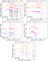 |
Fig. 2. Ultraviolet and optical light curves of SNe 2020nxt, 2020taz, 2021bbv, 2023utc, and 2024aej. The dashed vertical line marks the o/r-band maximum light as the reference epoch. The epochs of our spectra are marked with vertical solid red lines on the top. The upper limits are marked by empty symbols with arrows. For clarity, the light curves for the different bands are shifted with arbitrary constants as reported in the legend. Usually, magnitude errors are smaller than the symbols. |
No k-correction was applied to our photometric data, as all SNe in our sample are located in the local Universe (z < 0.1). To perform an accurate k-correction, comprehensive knowledge of the spectral evolution across all relevant phases is required, including the effects of reddening, to enable reliable interpolation between photometric bands. However, for our sample, the spectroscopic coverage is sparse and does not adequately span the full photometric wavelength range or temporal evolution. To avoid introducing additional systematic uncertainties due to these limitations, we refrained from applyingk-corrections.
3.2. Light curves and the comparison with other SNe Ibn
3.2.1. Apparent light curves
Our follow-up observations for each of the five SNe commenced shortly after their discovery and continued for several months. Figure 2 presents the apparent light curves of these events.
When the survey monitoring cadence is low, the explosion epoch of a new SN is usually assumed to be the midpoint between the last non-detection and the first detection. In the case of SN 2020nxt, the explosion time was estimated from the last non-detection in the o band (MJD = 59030.56) and the first detection in the c band (MJD = 59031.58), hence MJD = 59031.1 ± 0.5 days. In the case of SN 2021bbv, the explosion time was derived as the midpoint between the last non-detection in the c band (MJD = 59232.52) and the first detection in the g band (MJD = 59234.45), yielding MJD = 59233.5 ± 1.0 days. Similarly, for SN 2023utc, the explosion time was estimated to be at MJD = 60226.9 ± 2.5 days, based on the last non-detection (MJD = 60224.4) and the first detection (MJD = 60229.4), both in the ZTF g band.
Artificial neural networks (ANNs) are a widely adopted machine-learning technique, particularly well-suited for tasks involving regression and estimation. ReFANN25 is an ANN-based code that utilises a supervised learning procedure andconsists of three primary layers: input, hidden, and output (for further details, see Wang et al. 2020a, 2020b, 2021b). In Fig. 3, we show the reconstruction of the early-time light curve (from approximately two weeks past explosion) in the flux space using the ReFANN tool. This method provides an explosion epoch of  for SN 2020taz, and
  for SN 2024aej.
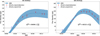 |
Fig. 3. Constraints on the explosion epochs of SNe 2020taz (left) and 2024aej (right). Early time ATLAS o-filter data are shown in the flux space. The zero flux level is marked by a horizontal dashed line. Red dots indicate real detections, while blue circles show the latest detection limit. |
To estimate the peak magnitude for SNe 2020nxt, 2020taz, 2023utc, and 2024aej, we used the ReFANN tool on the r-band or o-band light curve data, focusing on a period of approximately one week around the peak (see Fig. C.1 in Appendix C). In the case of SN 2020nxt, we obtained a peak magnitude of  on MJD = 59038.4
 . Similarly, for SN 2020taz, we derived a peak magnitude of
  on MJD = 59110.9
 . In the case of SN 2023utc, the peak magnitude is found to be
  on MJD = 60233.3
 , and for SN 2024aej, the peak magnitude is
  on MJD = 60328.1
 . Due to the lack of pre-peak data for SN 2021bbv, the peak time can only be estimated to be earlier than MJD = 59242.2, with a peak brightness of r ≤ 18.6 mag, which is likely close to the actual peak magnitude given the flat light curve observed at discovery in the r and i bands.
Additionally, we estimated the post-maximum decline rates of the five SNe across both UV and optical bands by performing linear regression fits on the post-peak data. These results, which offer a comparison of the fading behaviour in different wavelengths, are presented in Table D.1 (Appendix D). Given the observed changes in the slope of the light curves of SN 2020nxt at approximately +25 days and +45 days, we calculated the decline rates over three distinct time intervals. A minor scatter in the decline rates among the different filters can be noticed. The UV light curves exhibit a faster decline than the optical ones. During the first phase (e.g. γ0 − 25(g)=11.70 ± 0.34 mag per hundred days), the decline is steeper than in the second phase (e.g. γ25 − 45(g)=5.92 ± 0.59 mag per hundred days). In the last phase (e.g. γ45 − 60(g)=32.82 ± 2.15 mag per hundred days), the decline rate becomes significantly faster than in the first phase. An accelerated decline in optical luminosity during the late phases is a frequently observed in SNe Ibn (e.g. Mattila et al. 2008; Pastorello et al. 2015d; Wang et al. 2024a).
Following the rise to the o-band maximum, the light curves of SN 2020taz exhibit a plateau during the first 10 days followed by a magnitude decline with a rate of γ10 − 20(g)=9.75 ± 1.44 mag per hundred days. At later stages, the decline rate increases to γ20 − 30(g)=27.78 ± 3.25 mag per hundred days. We also note a difference in the decline rates across the different filters. Specifically, the redder light curves decline more slowly compared to the bluer ones. This trend is particularly pronounced during the early decline phase, as shown by the decline rate values reported in Table D.1 (Appendix D).
SN 2021bbv exhibits a linear decline until +25 days, with a rate of γ0 − 25(B)=10.15 ± 0.42 mag per hundred days. This initial phase is followed by a slightly slower linear decline with a rate of γ25 − 50(B)=5.97 ± 0.91 mag per hundred days. SN 2023utc exhibits a similar two-phase decline pattern as SN 2021bbv. In the case of SN 2024aej, observations are limited to the first 20 days past maximum, during which it shows a decline rate similar to the initial phase of SN 2021bbv and SN 2023utc, with γ0 − 20(B)=17.23 ± 0.80 mag per hundred days.
3.2.2. Colour curves
The colour evolution of the five SNe of our sample is compared in Fig. 4 with other Type Ibn events from the literature26. This comparison reveals a diversity in the colour evolution of SNe Ibn. In the case of SN 2020nxt, the B − V colour remains nearly constant, fluctuating around 0 mag throughout the observed period. Similarly, for SNe 2020taz and 2021bbv, the B − V colours remain close to 0.2 mag, resembling the early-stage behaviour of SN 2006jc. In contrast, SN 2023utc shows a more pronounced evolution in its B − V colour, increasing from approximately 0.3 mag at +10 days to around 0.7 mag by +20 days. At maximum light, SN 2024aej exhibits an initial B − V colour close to −0.1 mag, but it transitions towards redder colours, reaching B − V ∼ 0.7 mag by +20 days. The colour evolution of both SN 2023utc and SN 2024aej closely follows the early-stage evolution observed in ASASSN-15ed, SN 2010al,and SN 2014av.
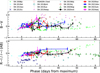 |
Fig. 4. Colour evolution of SNe 2020nxt, 2020nxt, 2021bbv, 2023utc, and 2024aej compared with a large sample of SNe Ibn from the literature. The colour curves have been corrected for Galactic extinction. |
In the case of SN 2020nxt, the r − i colour remains nearly constant around ≃0 mag between +5 and +40 days, resembling the behaviour of SN 2014av. However, at t ≳ +55 days, it shifts towards redder colours, reaching ∼0.3 mag. The r − i colour for SNe 2020taz, 2021bbv, and 2024aej slowly increases, suggesting a gradual temperature decrease over time. Specifically, for SN 2020taz, the r − i colour rises from −0.2 mag to 0.2 mag, while for SN 2021bbv it increases from −0.2 mag to 0.4 mag, and for SN 2024aej, it changes from −0.2 mag to 0.3 mag. The evolution of the R − I/r − i colour in these SNe is consistent with the trends observed in SNe 2010al, 2019kbj, and 2019uo, although the timescales can vary significantly among individual objects. In contrast with the other SNe Ibn and with its own B − V trend, the SN 2023utc r − i colour becomes bluer with time, from 0.1 mag to −0.3 mag.
3.2.3. Absolute magnitude light curves
After applying the corrections for distance and extinction as described in Section 2, we calculated the maximum absolute magnitude for SN 2020nxt to be Mo = −19.1 ± 0.1 mag. The peak absolute magnitudes of the other objects of the sample are: Mo = −17.8 ± 0.2 mag for SN 2020taz, Mr = −16.4 ± 0.5 mag for SN 2023utc, and Mr = −19.2 ± 0.1 mag for SN 2024aej. In the case of SN 2021bbv, only an upper limit of Mr < −18.8 mag can be inferred for the peak absolute magnitude in the r band (see Table 2).
Figure 5 shows a comparison of the absolute r-band light curves for a subset of SNe Ibn. When r-band observations are not available, light curves in adjacent bands are used for comparison. For instance, for OGLE-2012-SN-006 (hereafter OGLE12-006, Pastorello et al. 2015b), we used observations in the well-sampled I-band. SNe Ibn are usually quite luminous, with absolute r-band magnitudes between −18 and −20 mag. As shown in Fig. 5, the light-curve shapes of SNe Ibn are quite diverse. Comparing the r-band light curves of SNe 2020nxt, 2021bbv, and 2024aej with those of other SNe Ibn, we find that in most cases they follow the behaviour of the template presented by Hosseinzadeh et al. (2017) and Khakpash et al. (2024) at around the peak brightness. Following the initial rise, the light curve of SN 2020taz transitions into a plateau phase, similar to that observed in SN 2020bqj, which lasts approximately 10 days at an r-band absolute magnitude of −17.8 to −18.0 mag, placing it at the fainter end of the Type Ibn SN sample. SN 2023utc is an evident outlier, as it is the faintest Type Ibn SN discovered to date, with an extremely faint r-band absolute magnitude of only −16.4 mag. This is largely below the average absolute magnitude of SNe Ibn (Mr ∼ −19 mag; Pastorello et al. 2016), and also significantly fainter than the transitional Type IIn/Ibn SN 2005la (MR ∼ −17.2 mag; Pastorello et al. 2008b). The very faint absolute magnitude of SN 2023utc poses new questions regarding the possible progenitors stars and the explosion mechanisms of SNe Ibn.
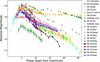 |
Fig. 5. Light curves of SNe 2020nxt, 2020taz, 2021bbv, 2023utc, and 2024aej in the R/r-band including the comparison SNe Ibn. The template r-band light curves for SNe Ibn are from Hosseinzadeh et al. (2017, yellow) and Khakpash et al. (2024, purple). |
3.2.4. Pseudo-bolometric light curves
A bolometric light curve can be derived by integrating the spectral energy distribution (SED) across the entire electromagnetic spectrum. However, in most cases, observations are not available for filters redder than the I/i band or bluer than the u band. Consequently, to facilitate reliable comparisons among SNe Ibn, we computed pseudo-bolometric light curves limited to the observed B through I/i bands. To obtain these, we first converted extinction-corrected magnitudes to flux densities and then integrated the SEDs at their effective wavelengths, under the assumption of negligible flux contributions outside this integration range. The resulting pseudo-bolometric light curves are shown in Fig. 6, and the peak luminosities are reported in Table 2. In most cases, the peak luminosities of our SN sample fall within the range of 3 × 1042 erg s−1 to 2 × 1043 erg s−1, with SN 2023utc being notably fainter at approximately 7 × 1041 erg s−1. The pseudo-bolometric light curve profiles of SNe 2020nxt, 2021bbv, 2023utc, and 2024aej show broad similarities to those of typical Type Ibn events (e.g. SN 2006jc and SN 2018jmt), as illustrated in Fig. 6. In contrast, the pseudo-bolometric light curve of SN 2020taz displays a distinctive plateau near the luminosity peak. A sudden drop at +40 days observed in the optical light curve of SN 2020nxt, accompanied by a redward colour shift, suggests a potential early dust formation in a cool dense shell, as observed in SN 2006jc (Mattila et al. 2008; Smith et al. 2008; Di Carlo et al. 2008).
Light-curve parameters for SNe Ibn.
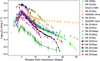 |
Fig. 6. Pseudo-bolometric light curves of SNe 2020nxt, 2020taz, 2021bbv, 2023utc, and 2024aej compared with those of a sample of SNe Ibn. |
To further analyse these light curves, we applied a non-parametric fit using the ReFANN code to reconstruct the pseudo-bolometric light curves and integrated them over the entirephotometric evolution, with integration limits defined by the time range of the available photometric data. The resulting radiated energies range from (1–32)×1048 erg, as listed in Table 2. These values should be interpreted as lower limits due to incomplete wavelength and temporal coverages.
To facilitate a meaningful comparison between SNe 2020nxt, 2020taz, 2021bbv, 2023utc, 2024aej, and the comparison star, we constructed their pseudo-bolometric light curves based on the observed wavelength range. To more accurately estimate the full bolometric light curves of these five SNe, we fitted the broad-band photometry with a blackbody model, extrapolating the luminosity contributions from the blackbody tails outside the observed range. Figure 7 shows, for each SN, representative blackbody fits to the SED at times near the peak luminosity. All five SEDs are well described by a single blackbody function. The evolution of the best-fitting blackbody temperatures and radii, along with the resulting bolometric luminosities, is presented in Figures 8 and 9 (for the latter, see discussion in Sect. 3.4). We note that we only focus primarily on the long-term evolution of the bolometric luminosity; short-duration fluctuations in the light curves are not captured in the final bolometric light curves.
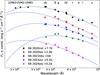 |
Fig. 7. Representative blackbody fits to the SEDs at epochs near the peak luminosity for each SN in our sample. The blue lines show the best-fitting blackbody functions. For visual clarity, the SEDs have been vertically offset by arbitrary constants. |
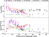 |
Fig. 8. Evolution of the blackbody temperature and radius for our SN sample. |
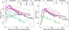 |
Fig. 9. Comparison between the bolometric light curves of the five SNe Ibn in our sample and representative interaction models from Dessart et al. (2022). The left panel displays simulations involving ejecta–wind interactions, while the right panel shows ejecta–ejecta interaction scenarios. |
Except for SN 2020nxt, our sample lacks UV observations, and this may significantly affect the robustness of our blackbody fits, particularly at early times. Arcavi (2022) explored the systematic uncertainties in constraining hot blackbody parameters using optical photometry alone and found that for blackbody temperatures exceeding ∼35 000 K, the inferred values may be overestimated by ∼10 000 K. Bolometric luminosities can be overestimated or underestimated by a factor ×3 − 5 at very high temperatures (above ∼60 000 K). However, as indicated by the relatively constant colours and the blackbodytemperatures derived from the spectra (see Section 4), the temperatures near and after the peak luminosity in our sample are typically below 20 000 K. These values are sufficiently low that the lack of UV data is unlikely to introduce significant systematic biases in the bolometric luminosity (Arcavi 2022). In practise, UV coverage is currently available for only a subset of SNe Ibn, mostly through Swift observations. For other SNe Ibn, including our sample, blackbody fitting to optical photometry remains a standard and widely accepted approach to estimate bolometric light curves (e.g. Shivvers et al. 2016; Karamehmetoglu et al. 2021; Gangopadhyay et al. 2022).
3.3. Modelling the multi-band light curves with the MOSFiT framework
The radioactive decay (RD) model of 56Ni, combined with circumstellar interaction (CSI), has been widely employed to interpret the light curves of SNe Ibn (e.g. Karamehmetoglu et al. 2017; Kool et al. 2021; Pellegrino et al. 2022; Ben-Ami et al. 2023). A robust and widely used tool to model light curve is the MOSFiT code (Guillochon et al. 2018), which has been successfully applied in recent studies of SNe Ibn (e.g. Kool et al. 2021; Farias et al. 2024). In this work, we utilised MOSFiT to fit the full multi-band light curves, making use of a Monte Carlo approach that yields statistically robust parameter uncertainties and self-consistent fits to all relevant variables. Crucially, MOSFiT accounts for the colour information by fitting each band independently.
The RD MOSFiT model describes any radioactive powering from the 56Ni decay through three key parameters: the nickel fraction (fNi), the γ-ray opacity of the ejecta (κγ), and the optical opacity (κ). In addition, the code allowed us to incorporate an ejecta–CSM interaction model with free parameters characterising both the ejecta and the surrounding medium (see Villar et al. 2017). These include the ejecta mass (Mej), the kinetic energy (Ekin), and the inner and outer density profiles of the ejecta (ρej, in ∝ r−δ and ρej, out ∝ r−n). The CSM is described by its inner radius (R0), the density (ρCSM), and the radial density profile (ρCSM ∝ r−s), where s = 0 corresponds to a constant-density shell and s = 2 represents a steady wind. MOSFiT also accounts for the explosion time (texp), defined as relative to the first photometric detection, and includes nuisance parameters such as the minimum allowed temperature of the photosphere (Tmin) and a white-noise term (σ) that is added in quadrature to the photometric uncertainties to assess the fit quality.
Although the model involves a high-dimensional parameter space, the key physical parameters of interest in this study are fNi, Mej, MCSM, Ekin, and R0. We fixed five model parameters to standard values: δ = 0, n = 12, s = 0, κ = 0.1 cm2 g−1 and κγ = 0.027 cm2 g−1. This resulted in a set of eight free parameters: fNi, Mej, MCSM, ρCSM, R0, Ekin, Tmin, and σ. To explore the parameter space efficiently, we employed the dynamic nested sampling algorithm implemented via the dynesty package (Speagle 2020), as recommended for complex models. We initialised the sampler with 120 live points (also referred to as ‘walkers’) and ran the algorithm until the default convergence criterion in dynesty was satisfied. This criterion ensures that the uncertainties in both the model evidence and the posterior distributions fall below predefined thresholds. The number of iterations required to reach convergence varies depending on the complexity of the light-curve data: approximately 760 000 iterations for SN 2020nxt, 210 000 for SN 2020taz, 180 000 for SN 2021bbv, 150 000 for SN 2023utc, and 110 000 for SN 2024aej.
Figure 10 presents the MOSFiT model light curves across the observed photometric bands, overplotted with the corresponding observational data. The best-fitting parameter values, which are most relevant to our analysis, are summarised in Table 3. All parameters are well constrained by the data, with uncertainties representing the 68% confidence intervals derived from the posterior distributions. Two parameters are omitted from the table: the noise term σ, which was consistently well constrained across the five samples (typically σ ∼ 0.2), and the final plateau temperature Tmin, to which the key physical parameters are relatively insensitive (Nicholl et al. 2017; Kool et al. 2021). The corner plots illustrating the posterior probability distributions and the correlations among parameters for the model fits are shown in Appendix E, Figs. E.1–E.5.
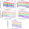 |
Fig. 10. Light curves from the RD+CSI model fitted to the multi-band photometry of five SNe Ibn using the Monte Carlo code MOSFiT. For each filter, a representative subset of model light curves randomly drawn from the posterior distributions is shown to illustrate the range of the model fits. The latest pre-discovery upper limits are indicated by triangles. |
Best-fit parameters for the RD+CSI model.
The inferred ejecta masses in our sample span a relatively narrow range, from a minimum of ∼0.85 M⊙ (SN 2023utc and SN 2024aej) to a maximum of ∼3.03 M⊙ (SN 2020taz). This upper edge is substantially lower than the average ejected mass of ∼16 M⊙ reported for some other SNe Ibn, including SN 2019uo (Gangopadhyay et al. 2020), PS15dpn (Wang & Li 2020), and SN 2020bqj (Kool et al. 2021). In contrast, the ejected masses derived for our events are broadly consistent with the theoretical maximum of ∼1.2 M⊙ predicted for typical SNe Ibn progenitor systems (single or binary) from radiative-transfer models (Dessart et al. 2022), and also fall within the ∼1–3 M⊙ grid explored in the analytical light-curve models by Pellegrino et al. (2022). The kinetic energies inferred for our sample span a wide range (EK ∼ (0.06–0.91)×1051 erg). These values are consistent with those estimated for other SNe Ibn, such as ∼0.35 ×1051 erg for SN 2023tsz (Warwick et al. 2025) and ∼1051 erg reported by Maeda & Moriya (2022), although SN 2023utc appears to represent a sort of lower limit for the kinetic energies observed in SNe Ibn. The estimated CSM masses lie in the range MCSM ∼ 0.17–0.95 M⊙, in agreement with prior estimates for similar events, including 0.2–1 M⊙ from Pellegrino et al. (2022), ∼0.73 M⊙ for SN 2019uo (Gangopadhyay et al. 2020), and ∼1.6 M⊙ for SN 2020bqj (Kool et al. 2021). The inner radii of the CSM shells are found to be RCSM ∼ 10–50 AU, with corresponding densities of ρCSM ∼ 10−10–10−7 g cm−3. The synthesised 56Ni masses, computed using MNi = Mej × fNi, are in the range 0.002–0.15 M⊙. These are consistent with ≤0.19 M⊙ reported by Pellegrino et al. (2022), as well as the ≤0.1 M⊙ reported by Maeda & Moriya (2022). Using the relation  , we estimate the ejecta velocities to lie in the range ∼2700–13 500 km s−1, consistent with the ∼3300 km s−1 measured for SN 2020bqj (Kool et al. 2021) and ∼11 300 km s−1 for SN 2019kbj (Ben-Ami et al. 2023).
3.4. Comparison with radiation-hydrodynamic interaction models
To investigate the interaction-powered scenarios relevant to SNe Ibn, Dessart et al. (2022) conducted one-dimensional multi-group radiation-hydrodynamics simulations using the HERACLES code. Their models comprise an inner shell representing the SN ejecta and an outer shell mimicking the CSM, formed either through explosive mass ejection or via a super-Eddington wind. By systematically varying the ejecta and CSM properties, they explored the resulting bolometric light curves focusing on the rise time, the peak luminosity, and the radiated energy during the high-luminosity phase. The fiducial inner ejecta model adopted Ekin = 7 × 1050 erg, Mej = 1.49 M⊙, and M(56Ni)=0.08 M⊙, with scaled-down variants to test lower-energy explosions. The outer shell configurations included both 1 M⊙ ejecta-like CSM with kinetic energies of 1047–1049 erg and wind-like CSM with a terminal velocity of v∞ = 1000 km s−1 and mass-loss rates spanning 10−3–10−1 M⊙ yr−1. These simulations yielded a broad range of light-curve morphologies and properties of the cold dense shell (CDS; see Table 1 of Dessart et al. 2022).
In Figure 9, we compare the bolometric light curves of the five SNe Ibn in our sample with representative interaction models from Dessart et al. (2022). The left panel shows simulations with ejecta–wind interaction, while the right panel presents ejecta–ejecta configurations, similar to those discussed in Woosley et al. (2021). It is important to note that the models from Dessart et al. (2022). are not tailored to reproduce individual events, but rather to explore the general behaviour of interacting transients across a wide parameter space. They highlight key observational features such as the rise time, the peak luminosity, and the time-integrated bolometric output during the high-luminosity phase, demonstrating how variations in ejecta and circumstellar medium properties produce diverse light-curve morphologies.
Their simulations show that standard-energy explosions of helium stars embedded in dense, wind-like CSM can reach peak luminosities of a few 1044 erg s−1 within a few days, similar to luminous events like AT 2018cow. Weaker winds, on the other hand, lead to Type Ibc-like transients with double-peaked light curves and more modest luminosities of ∼1042.2–1043 erg s−1. The observed rise time of ∼10 days in our Type Ibn SN sample suggests the need for relatively high mass-loss rates (Ṁ ≳ 0.1 M⊙ yr−1) to reproduce the light-curve shapes. For SN 2023utc, which showed a lower luminosity, models with reduced ejecta density or velocity may provide a more suitable match, as the shock power becomes less relevant and the luminosity accordingly diminishes. A viable configuration that accounts for both the radiative and kinematic properties of several objects in our sample (SNe 2020nxt, 2020taz, 2021bbv, and 2024aej) requires low-mass and low-energy ejecta colliding with a massive outer shell, as exemplified by models E1, E2, E5, or E6 in Dessart et al. (2022). This interaction scenario naturally explains the persistence of narrow spectral features and moderate luminosities. Such a setup may occur when a low-mass helium star in a binary system undergoes substantial envelope stripping via mass transfer, followed by a nuclear flash or enhanced wind phase shortly before the core collapse, and ultimately explodes with a relatively low kinetic energy. For SN 2023utc, an even lower-velocity or lower-density inner shell than those in current models is likely required to match the observed photometric evolution.
3.5. Correlations of the physical parameters
Comparing the properties of our five SNe with those of other SNe Ibn provides valuable insights for a more precise characterisation of this SN type. Wang et al. (2024a) presented a V-band phase-space diagram for SNe Ibn, suggesting the existence of correlations between peak magnitude, rise time, and decline rate. We extended this approach by examining both photometric observables and derived physical parameters for SNe Ibn. Specifically, we present in Fig. 11 the following phase-space diagrams: R/r-band peak magnitude versus rise time, R/r-band peak magnitude versus R/r-band decline rate, rise time versus R/r-band decline rate, peak bolometric luminosity (Lpeak) versus t0.5 (the time required for the luminosity to decline by half from peak), and ejecta kinetic energy (EK) versus synthesised 56Ni mass. Our new sample comprises SNe 2020nxt, 2020taz, 2021bbv, 2023utc, and 2024aej27. These comparisons allow us to place our events within the broader context of the Type Ibn SN population and to assess the extent to which the observed diversity is reflected in the explosion and physical parameters.
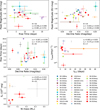 |
Fig. 11. Relationships between parameters inferred from the light curves of SNe Ibn. Top left: R/r-band peak magnitude versus rise time. Top right: R/r-band peak magnitude versus R/r-band decline rate. Centre left: Rise time versus R/r-band decline rate. Centre right: Peak luminosity (Lpeak) versus t0.5 (the time required for the luminosity to decline by half from its peak). Bottom left: Kinetic energy (EK) versus synthesised 56Ni mass. The weighted Pearson correlation coefficient (rP), the Spearman rank correlation coefficient (rS), and the associated p-values (probability of chance correlation) are provided for each parameter pair. Statistics exclude data points with rise time and peak magnitude limits. |
To quantify potential correlations among these parameters, we calculate the weighted Pearson correlation coefficient (rP), which accounts for the uncertainties under the assumption of Gaussian errors; the Spearman rank correlation coefficient (rS), which is non-parametric and equally weights all points; and the associated p-values (see Fig. 11). No statistically significant correlation is found between the peak magnitude and the rise time, or between the rise time and the decline rate. However, we observe a moderate negative correlation between the peak magnitude and the decline rate, indicating that more luminous events tend to evolve more rapidly after maximum light. No clear correlation is evident between Lpeak and t0.5, although most SNe Ibn exhibit t0.5 values in the range of 5–15 d and peak luminosities around 1043 erg s−1. A weak positive trend is apparent between the kinetic energy and the synthesised 56Ni mass, consistent with the finding of Pellegrino et al. (2024) that fainter, slower-evolving, interaction-powered transients generally exhibit lower explosion energies and produce less 56Ni.
As shown in Fig. 11, SN 2023utc displays a peak magnitude lower than those of most SNe Ibn, while the decline rate of SN 2020taz is comparable to those of SNe 2011hw and 2020bqj, both exhibiting slower rates. In contrast to the extreme phase-space locations of SNe 2023utc and 2020taz, SNe 2020nxt, 2021bbv, and 2024aej occupy central positions in the diagrams, suggesting that they represent more typical events within the Ibn sample.
4. Spectroscopy
Our spectral sequences for SNe 2020nxt, 2020taz, 2021bbv, 2023utc and 2024aej were obtained using multiple instrumental configurations, which are listed in Table B.1 (Appendix B). Basic parameters for the spectra are reported in Tables F.1–F.5 (Appendix F).
The spectral data were processed using standard procedures, combining IRAF tool and optimised pipelines like FLOYDS28, depending on the instrumental configuration and observatory setup. The preliminary reduction steps included corrections for bias, overscan, and flat-fielding of the two-dimensional frames to account for specific instrumental effects. Subsequently, the 1D spectra were optimally extracted, ensuring a robust S/N ratio for the target spectra. Wavelength calibration was performed using arc lamp spectra obtained during the same observing run and instrumental configuration as the science data. Night-sky emission lines were cross-checked to refine the wavelength solution. Flux calibration was achieved using spectrophotometric standard stars observed under similar conditions. A sensitivity function derived from the standard star spectra was applied to the transient’s spectra. To ensure consistency, the flux-calibrated spectra were compared against coeval broadband photometric data, and correction factors were applied in cases of significant discrepancies. Finally, the strongest telluric absorption bands, primarily from O2 and H2O, were removed using spectra of early-type standard stars, which exhibit a nearly featureless continuum in the telluric absorption regions. The fully processed spectra, presented in Fig. 12, provide a robust basis for analysing the properties of the five Type Ibn SN.
 |
Fig. 12. Spectral sequences of the five SNe Ibn. The dashed vertical lines indicate the main H and He I transitions, while the ⊕ symbol marks the strongest telluric absorption bands. All spectra have been corrected for redshift and extinction. Grey lines represent smoothed spectra (originally with a lower S/N) processed with a Savitzky-Golay filter. |
4.1. Spectroscopic evolution and line identification
4.1.1. SN 2020nxt
– Wang et al. (2024b) reported 19 spectra for this object; we supplemented the available dataset with ten additional spectra. Our spectral sequence is shown in Fig. 12. Over the entire observational period, the spectra exhibit a moderateevolution.
The first spectrum (phase +5.7 d), previously reported by Srivastav et al. (2020) and Wang et al. (2024b), is the classification spectrum. It shows a blue pseudo-continuum, and a blackbody fit to it yields a photospheric temperature of TBB = 11 800 ± 3300 K. In the second spectrum (phase +9.7 d), the blackbody temperature increases to TBB = 17 500 ± 6200 K. The third spectrum (phase +11.7 d) lacks sufficient blue-wavelength coverage, making the temperature fit unreliable. The fourth to tenth spectra (taken at phases +13.5, +15.7, +16.8, +22.7, +28.5, +28.7, and +38.8 d) show minimal evolution, with temperatures fluctuating between 11 000 and 14 000 K. The last spectrum (phase +43.7 d) still displays a blue continuum, with the temperature decreasing to TBB = 9700 ± 3500 K.
In Fig. 12, we mark the strongest He I lines and the lines of the Balmer series. The He I lines, particularly He I λ5876 and λ7065, are the most prominent features in the spectra of SN 2020nxt. Additionally, a weak and narrow Hα line with a P Cygni profile is observed in the first three spectra, with an absorption minimum blue-shifted by approximately 100 − 300 km s−1. However, other prominent Balmer lines typical of Type IIn SNe are not securely detected in SN 2020nxt.
We conducted a detailed line identification using the spectrum with the highest S/N ratio, obtained at phase +16.8 d (Fig. 13). This spectrum exhibits several broad bump features, including the following:
-
7600–8000 Å: a blend of O I λ7774 and Mg II λλ7877 − 7896;
-
8100–8300 Å: Mg II λλ8214 − 8235;
-
8300–8800 Å: a blend including O I λ8446 and the near-infrared Ca II triplet;
-
9000–9400 Å: a blend including C I λλ9095 − 9112, Mg II λλ9218 − 9244, and O I λλ9261 − 9266;
-
4450–4650 Å: likely a blend including He I λ4471, Mg I] λ4571, and Fe II λλ4303 − 4352;
-
5100–5400 Å: likely a blend including C II λ5145 and Fe II λλ5018, 5169, 5198, 5235.
We also tentatively identified features at λ5680 and λ6482 as N II and [Ca II] λλ7292, 7324. Whilst these features are usually expected in CC SNe, we do not securely detect lines typical of thermonuclear SNe, such as S II and Si II.
4.1.2. SN 2020taz
– The very rapid evolution and the modest apparent magnitude of SN 2020taz limited its spectroscopic monitoring to only five epochs. The first spectrum (phase +5.5 d) is the blue continuum-dominated classification spectrum, with a blackbody temperature of TBB = 15 000 ± 3500 K. Its main features include He I lines (λ5876, λ6678, λ7065) with P Cygni profiles and velocities of approximately 800 km s−1, as well as a weak P Cygni Hα line.
The second and third spectra (phases +8.1 d and +11.0 d, respectively) show a redder continuum with a decreasing blackbody temperature of approximately TBB ∼ 11 400 K, while the Hα feature becomes more prominent with time. The fourth spectrum (phase +24.0 d) has a low S/N ratio and shows a significantly cooler temperature of TBB = 6700 ± 1800 K. The final spectrum (phase +29.0 d) reveals an increase in the prominence of the Hα line, with a P Cygni absorption minimum blue-shifted by ∼800 km s−1. Weak Hβ and Hγ lines are also detected, while the blackbody temperature increases slightly to TBB = 7400 ± 2200 K.
Similar to the Type Ibn prototype SN 2006jc (Foley et al. 2007; Pastorello et al. 2007; Smith et al. 2008; Mattila et al. 2008), SN 2020taz exhibits a very weak (almost undetectable) Hα line during the early phases, which becomes more pronounced only at later epochs. In contrast, Type IIn SNe typically display a narrow Hα line (FWHM ≤ 1000 km s−1) that dominates in strength the He I lines at all phases.
4.1.3. SN 2021bbv
– The four spectra of SN 2021bbv exhibit predominantly a blue continuum, with the photospheric temperature gradually decreasing from TBB ∼ 14 000 K to 8600 K. The prominent features in the spectra include the He I lines (λλ5876, 6678, 7065), which become more pronounced over time. The evolution of the He I line velocities is modest; this is discussed in detail in Section 4.3. For a more detailed identification of the spectral lines, we used the third spectrum (phase +11.8 d; see Fig. 13). Broad features, similar to those observed in SN 2020nxt, are detected at 4450 − 4650 Å, 5100 − 5400 Å, and 7600 − 8000 Å. However, the NIR Ca II triplet was not securely identified. Furthermore, we were unable to confidently identify the Balmer series lines or spectral features typical of thermonuclear SNe, such as S II and Si II.
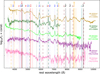 |
Fig. 13. Line identification in the highest-resolution late-time spectra of the five SNe presented in this paper. Spectra have been corrected for redshift and reddening, with indicated phases from the maximum light. |
4.1.4. SN 2023utc
– The four noisy spectra show a blue continuum, with the strongest feature being He Iλ5876. The photospheric temperature initially increases, and then decreases over time: TBB = 11 900 ± 5900 K in the first spectrum (phase +7.5 d), it peaks at TBB = 15 600 ± 2900 K in the second spectrum (phase +11.2 d), and declines to TBB = 4800 ± 1300 K in the last spectrum (phase +27.3 d). For the line identification, the third higher S/N spectrum (phase +16.3 d) was considered (see Fig. 13). We identify Hα, Hβ, Hγ, and He I λλ4471, 4921, 5016, 5876, 6678, 7065, 7281. However, alternative identifications for some features, such as C II λ6578, N II λ4803 and [Ca II] λλ7291, 7324, cannot be ruled out.
4.1.5. SN 2024aej
– Figure 12 shows that SN 2024aej exhibits spectral properties similar to those of SN 2023utc. Four spectra were obtained, all quite noisy ratios. They show a blue continuum dominated by prominent He I lines typical of SNe Ibn. Due to the low S/N, additional spectral lines cannot be securely identified (see Fig. 13). The photospheric temperature evolves from TBB = 15 600 ± 3000 K in the first spectrum (phase +1.2 d), to a peak of TBB = 17 800 ± 3600 K in the second spectrum (phase +3.2 d), before decreasing to TBB = 10 500 ± 2100 K in the final spectrum (phase +16.1 d).
4.2. Comparison of Type Ibn SN spectra
In Fig. 14, we compare the spectra of SNe 2020nxt, 2020taz, 2021bbv, 2023utc, and 2024aej obtained near the maximum light and at late phases with those of other SNe Ibn at similar phases. In the top part of Fig. 14, the spectra of these five SNe near peak brightness are compared to those of SNe 2006jc, 2010al, and 2019cj. The spectra of SNe Ibn exhibit remarkably similar blue continua with prominent He I lines in emission. However, subtle differences are also present. Specifically, Hα emission is weak but detectable in the spectra of SNe 2006jc, 2010al, 2020nxt, 2020taz, and 2023utc, while its presence is uncertain in SNe 2021bbv, 2024aej, and 2019cj. None of the objects exhibit clear flash-ionisation features. However, it should be emphasised that the earliest spectrum of our five events was obtained only after maximum light, later than the timing when flash-ionisation features were observed in other Ibn events. For instance, in SN 2010al (Pastorello et al. 2015a), flash-ionisation features appeared 8 days before the maximum light and disappeared 4 days later. Similarly, in SN 2019cj (Wang et al. 2024a), prominent flash features were observed 2.1 days before maximum. Therefore, given the timing of the earliest spectra for these five SNe, we cannot rule out the presence of flash-ionisation features at earlier stages.
In the lower part of Fig. 14, we compare the last spectra of SNe 2020nxt, 2020taz, 2021bbv, 2023utc, and 2024aej with those of SNe 2006jc, 2010al, and 2020bqj at similar phases. At late times, the emission lines become more prominent, allowing for a more reliable spectral identification. SNe 2020nxt, 2020taz, 2023utc, 2006jc, and 2020bqj show strikingly similar features, including prominent He I lines. A notable characteristic shared by these events is the absorption feature in the 4600–5200 Å region, which is likely due to Fe II line absorptions. A similar feature is also observed in stripped-envelope SNe. The blue pseudo-continuum and the decrease in flux beyond 5400 Å appear to be common features among most interaction-powered CC SNe, and is due to a blend of prominent emission lines of Fe (Smith et al. 2012; Stritzinger et al. 2012; Pastorello et al. 2015a). Although some heterogeneity exists within the Type Ibn SN population, their spectra generally exhibit consistent pseudo-continuum shapes, as well as line identification and profiles. This suggests that the physical conditions in the line-forming regions of the CSM are not significantly different among these SNe.
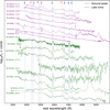 |
Fig. 14. Comparison of around-peak (purple) and late-time (green) spectra of SNe 2020nxt, 2020taz, 2021bbv, 2023utc, and 2024aej with other SNe Ibn at similar phases. All spectra have been corrected for redshift and extinction. Significant He I features are marked by blue dashed lines, while Balmer features by red dashed lines. |
4.3. Velocity evolution of the He I lines
To constrain the properties of the stellar wind and the nature of the line-emitting regions, we examine the velocity evolution of spectral lines. SNe powered by interaction typically exhibits lines with multiple-width components, originating from gas located in different regions (Chevalier & Fransson 1994; Chugai 1997; Pastorello et al. 2016). The narrow lines (with velocities ranging from a few hundred to ≤2000 km s−1) are likely produced in the unshocked CSM, constituted by material lost by the progenitor star prior to the SN explosion. Broader components, with typical velocities ranging from several thousand to ∼104 km s−1, are likely produced in shocked gas regions, distinct from the electron-scattering wings often observed in interacting SNe.
Following Pastorello et al. (2016), the velocity of the He-rich ejecta can be determined by measuring the wavelength of the blue-shifted absorption core of the P Cygni profile, when such a profile is clearly identified. If a P Cygni profile is not detected, the velocity is roughly estimated from the FWHM of the He I emission line. The FWHM is derived after the line profile has been deblended using a combination of Gaussian and Lorentzian fitting functions. The evolution of the narrow and the broader components of the He I lines for the SN sample is presented in Fig. 15. For SNe 2023utc and 2024aej, the noisy spectra prevent the measured velocities from accurately constraining the true physical properties of the gas.
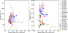 |
Fig. 15. Evolution of He I line velocities. Left panel: Temporal evolution of the velocities associated with the narrow He I line components, which trace the unshocked CSM. Right panel: Velocity evolution of the broader He I emission components, reflecting the dynamics of the shocked gas region. Data for comparison SNe Ibn are adopted from Pastorello et al. (2016) and Wang et al. (2024a). |
The velocity of the narrow He I components attributed to the unshocked CSM is a proxy for the stellar wind velocity prior to the SN explosion. Fig. 15 shows that the velocities of the narrow He I lines in the Type Ibn SN sample span a wide range of values, from a few hundred to approximately 2500 km s−1. However, while SNe 2005al, 2011hw, and PS1-12sk exhibit very low wind velocities (below 500 km s−1), more frequently the narrow He I components have velocities ranging from 500 to 1500 km s−1. In most cases, the narrow-line velocities exhibit a temporal growth: in SN 2020nxt the vFWHM increased from 900 km s−1 to 1300 km s−1, while in SN 2010al the P Cygni velocity rose from 1000 km s−1 to 1500 km s−1. Occasionally, the line velocities showed a negligible evolution with time, like in the cases of SNe 2020taz and 2021bbv, where the line velocities remained relatively stable at around 700 km s−1. These differences may suggest distinct progenitor, mass-loss and interaction scenarios.
The velocity evolution of the broader components of He I lines is also shown in Fig. 15. These broader components exhibited more pronounced temporal changes, reflecting heterogeneity in the ejecta velocities and in the density profiles of the interacting material. In some cases, the velocities of broader He I components increased over time. For instance, in SN 2005la the gas velocity rose from approximately 2000 km s−1 shortly after discovery to around 4200 km s−1 three weeks later. Similarly, in SN 2020taz vFWHM increased from 1700 km s−1 to 2500 km s−1. In contrast, some cases exhibited a narrowing trend over time. For example, in SN 2006jc the intermediate components of He I lines decreased from 3100 km s−1 to 1700 km s−1 in four months. This trend was also observed in other obejcts (SNe 2000er, 2002ao, 2014av; Pastorello et al. 2016). This was also observed in some SNe of our sample (SNe 2020nxt and 2021bbv), suggesting a decline in the velocity of the shocked gas region, likely caused by increasing density in the CSM gas distribution. A non-monotonic trend was seen in SN 2011hw, where the broader components velocity initially increased from 1900 km s−1 to 2500 km s−1, before declining to approximately 1600 km s−1 by ∼60 days post-maximum. Such peculiar evolution could be attributed to a complex density distribution in the shocked gas region.
4.4. Modelling the spectra
To constrain the progenitor and ejecta properties for our SNe Ibn sample, we compare observed spectral sequences with a set of non-local thermodynamic equilibrium (NLTE) radiative-transfer simulations computed using CMFGEN. These include models from Dessart et al. (2022), along with a few additional models with adjusted parameters (Dessart, priv. comm.). The simulations assume interaction between low-mass (≲1 M⊙), moderate-energy (∼1050 erg) ejecta and a slowly expanding, He-richcircumstellar shell of comparable mass. A dense, thin CDS forms as a result of this interaction and dominates the emission at late times.
In this quasi-steady configuration, hydrodynamical evolution is neglected, and the CDS is treated as a chemically mixed zone with a Gaussian density profile centred at 2000 km s−1 and rescaled to match the total ejected mass. The energy from the RD and the residual interaction is non-thermally deposited into the CDS, allowing an accurate treatment of the ionisation and excitation conditions. Although these simulations are not tailored to specific SNe, they allow us to explore of spectral diversity and parameter degeneracies. Notably, Dessart et al. (2022) demonstrated that similar spectral features can result from different combinations of CDS mass, radius, and input power.
The persistent presence of He I lines throughout the spectral evolution suggests a helium-rich progenitor. Following the approach of Wang et al. (2024b), we adopt helium-rich progenitor models for our analysis. Based on the helium-star evolutionary models of Woosley (2019), progenitors with the zero-age helium core masses between 3–4 M⊙ (e.g. models he3 and he4) are appropriate for reproducing the observational characteristics of SNe Ibn. For this study, we employ model he4, which is characterised by a total mass of 1.62 M⊙, comprising 0.92 M⊙ of helium, 0.31 M⊙ of oxygen, 0.03 M⊙ of magnesium, 0.0014 M⊙ of calcium, and assumes solar metallicity. Figure 16 presents a comparison between synthetic spectra from model he4p0 and observed spectra of five SNe Ibn at multiple epochs after the maximum light. To isolate the effect of the luminosity evolution, only the power varies with time, while the CDS radius (3 × 1015 cm) and velocity (2000 km s−1) are fixed. This simplification enables a broad comparison with observed spectralevolution, although we note that adopting a time-dependent composition would better capture specific line changes. These power values are broadly consistent with the bolometric light curve inferred from observations (see Fig. 9).
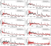 |
Fig. 16. Comparison between synthetic spectra from model he4p0 and observed spectra of five SNe Ibn at multiple epochs after bolometric maximum light. No smoothing has been applied to either the observed or modelled spectra. The synthetic spectra are based on simulations from Dessart et al. (2022) and Wang et al. (2024b) as well as newly computed models incorporating updated parameters. |
The radiative-transfer models presented by Dessart et al. (2022) are not designed to reproduce individual SNe Ibn, but instead aim to explore the general spectral diversity arising from ejecta-CSM interaction across a broad parameter space. As such, their applicability to specific events remains limited. A notable example of this limitation lies in the prediction of strong Fe II emission features blueward of 5500 Å in most models that do not assume nearly pure helium composition. However, such features were absent in several observed SNe Ibn, including the 11.0 d spectrum of SN 2020taz and the 16.3 d spectrum of SN 2023utc. The presence of a well-defined continuum and the absence of Fe II lines in these early spectra implied a dense and hot environment, inconsistent with the relatively cool, optically thin conditions required for Fe II emission. These discrepancies suggest that the underlying assumptions of a quasi-steady, dense shell configuration may not hold at early phases, when the ejecta and CSM have not yet formed a coherent, shocked shell. In such cases, models with a smaller shell radius and a higher power, implying higher density and temperature, are likely to provide a more accurate representation of the ionisation conditions (as shown in Appendix G, Fig. G.1, where a model with a reduced radius better reproduced the observed spectra of SN 2020taz). However, the modelling framework adopted by Dessart et al. (2022) does not accommodate this early-time hydrodynamical evolution. Therefore, caution must be adopted when interpreting early-time spectra using these models, and alternative approaches incorporating time-dependent hydrodynamics may be required to fully capture the physical conditions in the pre-shock or early interaction stages.
The models of Dessart et al. (2022) do not include hydrogen and therefore fail to reproduce Balmer lines such as the prominent Hα feature observed in the 29.0 d spectrum of SN 2020taz. The presence of hydrogen can significantly modify the ionisation balance and increase the optical depth, thereby affecting the emergent spectrum. Additionally, synthetic spectral lines in these models are sometimes broader than those observed. This mismatch may be attenuated by adopting lower velocities for the CDS in tailored models, which would yield narrower features while preserving the overall spectral morphology. Another recurring discrepancy is the presence of central absorption dips in several He I lines (e.g. He I λ5876) in the synthetic spectra. These features arise due to a marginal optical thickness in the shell and are not frequently present in the observed spectra of SNe Ibn. Their absence may reflect small-scale asymmetries or clumping in the real ejecta-CSM interaction region, which are not captured by the current spherically symmetric, one-dimensional modelling approach. Incorporating multidimensional effects or introducing shell inhomogeneities may help resolve this tension.
A detailed analysis of SN 2020nxt has already been presented by Wang et al. (2024b), and our results are broadly consistent with their findings. Here, we briefly summarise a few key aspects. Synthetic spectra computed at 13.5, 16.8, 28.7, and 38.8 d post-maximum, using power inputs from 4 × 1042 to 5 × 1041 erg s−1, do not reproduce the temporal strengthening of the Ca II near-infrared triplet due to decreasing ionisation and optical depth. This feature, absent in the models of Dessart et al. (2022), is explained here as an ionisation effect rather than a calcium overabundance. While Mg II lines are consistently overestimated, their declining strength with time is qualitatively captured. Additionally, models underestimated the strength of metal lines blueward of 5300 Å in SN 2020nxt at 13.5 d, while overestimated them in the 19.9 d spectrum of SN 2021bbv. Although some discrepancies remain in reproducing individual features, the overall spectral evolution is broadly consistent with observations, supporting the scenario of ejecta–CSM interaction in SNe Ibn.
5. Discussion and concluding remarks
5.1. Observables and physical parameters
In this paper, a detailed analysis of the photometric and spectroscopic properties of five SNe Ibn is presented. The main outcomes can be summarised as follows:
-
The rise times of the light curves to maximum brightness for the five SNe Ibn range from 6 to 12 days, which is typical within the Type Ibn SN population (see Fig. 11 and Table 2).
-
At maximum light, our sample exhibits a wide range of luminosities, with peak magnitudes spanning from Mr ∼ −16 mag for SN 2023utc to Mr ∼ −19 mag for SN 2024aej. These provide pseudo-bolometric luminosities in the range of (1–10)×1042 erg s−1 and radiated energies (1–10)×1048 erg, with light curve durations spanning25–170 days.
-
The post-peak light curve decline shows two distinct trends. In some cases, the decline is initially steep, with rates of γ(r)≈9–16 mag (100 days)−1, and followed by a slower decline with γ(r)≈4–7 mag (100 days)−1, such as for SN 2020nxt, SN 2021bbv, and SN 2023utc (see Section 3.2.1). In other cases, a shallow plateau phase is observed at early phases (resembling the one observed in SN 2020bqj; Kool et al. 2021) and followed by a faster decline (e.g. SN 2020bqj with γ(r)≈5.5 mag (100 days)−1 and SN 2020taz with γ(r)≈24 mag (100 days)−1).
-
The colour evolution of our sample is consistent with what has been observed in other SNe Ibn. The nearly constant colour observed in most SNe Ibn is indicative of the little temperature evolution across this SN type, although with some exceptions (see Fig. 4). The similar colour evolution may reflect a shared power source in the Type Ibn SN sample driven by a sustained interaction between the ejecta and the CSM.
-
We performed multi-band light-curve modelling using MOSFiT, adopting the RD+CSI framework to constrain the properties of both the ejecta and the CSM. The inferred ejecta masses (Mej) span a relatively broad range of ∼1–3 M⊙, with corresponding kinetic energies (EKin) on the order of (0.1–1)×1051 erg. For the CSM, the shock-swept mass (MCSM) is estimated to lie between ∼0.2 and 1 M⊙, with inner radii in the range of ∼10–50 AU. The upper limits on the synthesised 56Ni mass for all five SNe Ibn in our sample are ≲0.2 M⊙, which is consistent with values inferred for other SNe Ibn in the literature (e.g. Pellegrino et al. 2022; Kool et al. 2021; Farias et al. 2024). We note a general trend whereby fainter and more slowly evolving SNe Ibn tend to exhibit lower explosion energies–regulated primarily by the ejecta mass (Mej) and velocity (vej)–as well as reduced amounts of synthesised 56Ni.
-
Spectroscopically, the sample exhibits relatively slow spectral evolution characterised by a hot blue continuum with superimposed prominent He I emission lines. Most spectra exhibit blackbody temperatures exceeding 10 000 K during the early phases, with a decline at later stages. Narrow He I lines, indicative of unshocked CSM, exhibit velocities of ∼1000 km s−1. In some cases, such as SN 2020nxt, a weak and narrow Hα line with a P Cygni profile (v ∼ 100–300 km s−1) is detected. However, other Balmer lines as well as spectral features typical of thermonuclear SNe are absent or very weak. A common characteristic of the sample is the dominance of a blue pseudo-continuum in the mid- to late-time spectra, which is accompanied by a significant flux decline beyond 5400 Å.
5.2. Progenitor and explosion scenarios
Despite several plausible scenarios proposed to explain the origins of SNe Ibn, their exact nature remains debated (Pastorello et al. 2007; Sanders et al. 2013; Maund et al. 2016). Hypotheses include thermonuclear explosions of helium white dwarfs, core collapse events from moderate-mass helium stars in binary systems (Maund et al. 2016; Sun et al. 2020), and the explosions of massive WR stars (Pastorello et al. 2007; Maeda & Moriya 2022).
5.2.1. Thermonuclear explosions of helium white dwarfs
The He-shell detonation on a white dwarf (sometimes labelled as type .Ia SN explosions) would potentially explain some of the properties observed in our sample. Our events belong to the well-populated group of fast-evolving SNe Ibn, with most exhibiting rise times of less than 10 days. Candidate SNe .Ia, such as SN 2002bj (Poznanski et al. 2010), are also fast-evolving He-rich transients with rapid light-curve evolution characterised by rise times of 1 − 6 days. Notably, dimmer type .Ia SNe tend to exhibit faster rises. Their peak magnitudes, ranging from MV ∼ −15 to −18 mag (Perets et al. 2010, 2011; Kasliwal et al. 2010; Fesen et al. 2017) are comparable to that of the faintest member of our sample, SN 2023utc.
On the other hand, other parameters determined for our sample, including the ejecta mass and the CSM properties, are inconsistent with the expectations for explosions originating from very low progenitor masses, such as thermonuclear SNe from helium white dwarfs. Another argument against the white dwarf detonation scenario is the absence of spectroscopic features typically associated with Type Ia SNe, such as prominent S II and Si II lines. For these reasons, we conclude that our sample is inconsistent with being thermonuclear explosions of He white dwarfs.
5.2.2. Core-collapse SNe from moderate-mass He stars in binary systems
While a thermonuclear origin cannot be definitely ruled out for a fraction of SNe Ibn (see Sect. 5.2.1, and discussion in Sanders et al. 2013), observational evidences suggest that most SNe Ibn are interacting CC SNe. In particular, the analysis of the spectra can provide key evidence for interpreting the explosion scenario. The spectral features identified in Fig. 13 exhibit some similarity with CC SNe transitioning to the nebular phase. While the [O I] λλ6300, 6364 doublet is not definitively detected, the enhanced He I λ7281 line may be attributed to the emergence of the [Ca II] λλ7291, 7324 doublet, a hallmark feature of CC SNe in their nebular phase. While ongoing CSM interaction may inhibit the detection of the [O I] λλ6300, 6364 doublet (as suggested for Type IIn SNe similar to SN 2009ip; see e.g. Brennan et al. 2022), its weakness may also be due to the lower mass of the progenitor’s core. A plausible scenario for our sample is that they originate from the explosions of moderate-mass (MZAMS < 20 M⊙ −25 M⊙) He stars in binary systems, producing partially stripped CC SNe. This interpretation is supported by the studies of recent SNe Ibn.
Sun et al. (2020) detected a point source at the location of the prototypical Type Ibn SN 2006jc with the HST at late times. They identified it as the surviving binary companion with an estimated initial mass of  , with the primary being only slightly more massive. This finding suggests that SNe Ibn may arise from interacting binary systems with moderate-mass progenitors. Additionally, we observed that most SNe Ibn occupy a confined region in the relationships between light curve parameters, as shown in Fig. 11, indicating some degree of homogeneity in the progenitor properties and hence the explosion scenario.
Furthermore, recent studies of SN 2023fyq have provided compelling evidence for a binary-origin scenario involving a low-mass helium star and a compact companion. Dong et al. (2024) reported a three-year-long precursor activity prior to the explosion, followed by a double-peaked post-explosion light curve with a peak luminosity of ∼1043 erg s−1. They interpret the precursor emission as a consequence of unstable mass transfer in a close binary system, which leads to the formation of a massive (∼0.6 M⊙) equatorial disc. The interaction between the SN ejecta and this disc is proposed to power the second peak in the light curve. The early-time light curve suggests the presence of dense, extended material (∼0.3 M⊙ at ∼3000 R⊙), likely ejected weeks before core collapse due to either silicon-burning instabilities or binary-driven mass loss. Tsuna et al. (2024) provide further support for this scenario by modelling the binary interaction between a ∼2.5–3 M⊙ helium star and a neutron star. Their simulations show that super-Eddington accretion onto the compact object can drive a long-lasting wind, producing optical/UV transients with luminosities of ∼1040–1041 erg s−1 over several years, consistent with the observed precursor of SN 2023fyq. The final explosion–either due to core collapse or a merger–produces an interaction-powered transient with characteristics resembling those of SNe Ibn. Although none of the SNe Ibn in our sample shows evidence of pre-explosion outbursts or double-peaked light curves, their spectral features and light-curve properties–such as peak magnitudes and post-maximum decline rates–are broadly consistent with the expectations from binary-interaction scenarios. This suggests that they may represent a different manifestation of binary evolution leading to the Type Ibn phenomenon.
Additional insights supporting moderate-mass He progenitor systems for most SNe Ibn are given by Wang et al. (2024b), who performed radiative-transfer simulations on the spectral evolution of SN 2020nxt. Their results suggest that its progenitor was a 4 M⊙ He-star that lost ∼1 M⊙ of its He-rich envelope prior to the explosion, implying an interacting binary system, which is in line with the outcomes of our modelling in Sect. 3.3.
Finally, Dessart et al. (2022) investigated the light-curve and spectral properties of SNe Ibn by performing both radiation-hydrodynamics simulations and NLTE radiative-transfer calculations, using the results of the former primarily to inform the initial conditions of the latter. The narrow spectral lines and moderate peak luminosities observed in most SNe Ibn suggest that they originate from low-energy explosions of relatively low-mass (≲5 M⊙) helium stars, likely in interacting binary systems. These progenitors are thought to collide with a dense helium-rich CSM, possibly of ejecta origin, located at a radius of ∼1015 cm. The NLTE radiative-transfer models for the resulting slow-moving dense shell formed and powered by ejecta-CSM interaction show good agreement with the late-time spectra of several SNe Ibn, such as SN 2006jc, SN 2011hw, and SN 2018bcc. These models favour a shell composition of approximately 50% helium, solar metallicity, and a total ejecta plus CSM mass of 1–2 M⊙. A lower helium fraction in the shell suppresses He I lines, thus disfavouring higher-mass configurations for typical SNe Ibn. Our bolometric light curves and spectral sequences are broadly consistent with the predictions from the Dessart et al. (2022) models, supporting the applicability of their framework to our Type Ibn SN sample.
5.2.3. The explosions of massive WR stars
Another possible origin for SNe Ibn is the explosion of higher-mass (MZAMS > 25 M⊙) WR stars. This scenario provides a straightforward interpretation of the typical CSM composition and velocities observed in SNe Ibn as well as the mass-loss events occurring prior to the explosion. Key evidence supporting this interpretation is the wind velocity of ∼1000 km s−1 inferred for our SN sample, which is consistent with the speeds expected in WR stellar winds. Several studies have suggested that WR stars may experience fallback during their explosions, leading to the production of little or no 56Ni (Woosley & Weaver 1995; Zampieri et al. 1998; Maeda et al. 2007; Moriya et al. 2010). Furthermore, the absence of [O I] λλ6300, 6364 lines in late-time spectra, as noted by Valenti et al. (2009), is an argument that has been used to support fallback in the explosion of very massive stars.
Massive stars with initial masses exceeding ∼18 M⊙ can lose significant amounts of mass via strong stellar winds without requiring a binary companion, and they leave behind a C + O core surrounded by a He-rich CSM (Heger et al. 2003; Langer 2012). Stars with even larger masses (70–140 M⊙) may undergo pulsational pair-instability (PPI) events. In particular, some PPI models have been shown to reasonably reproduce the light curves of SNe Ibn (Woosley 2017; Karamehmetoglu et al. 2021). However, a major challenge to this interpretation is that our sample appears to consist of single SN-like events without evidence of prior eruptions. Pre-SN outbursts have been observed in only a handful of SNe Ibn, such as SN 2006jc (Pastorello et al. 2007), SN 2019uo (Strotjohann et al. 2021), SN 2022pda (Cai et al., in prep.), SN 2023fyq (Brennan et al. 2024), and the transitional Type Ibn/IIn SN 2021foa (Reguitti et al. 2022; Farias et al. 2024). Unfortunately, as our sample is located in distant galaxies, we lack direct evidence of the progenitor stars and observations deep enough to capture their pre-explosion activity.
5.3. Concluding remarks
The available dataset for our sample does not provide sufficient constraints to definitively determine the progenitor masses or the explosion mechanisms of SNe Ibn. However, several lines of evidence suggest that in most cases, these events are terminal CC SNe originating from massive stars. Whether the progenitors are high-mass WR stars or lower-mass helium stars in binary systems remains an open question. Future observational facilities, such as the Chinese Space Station Telescope29 and the Vera C. Rubin Observatory30, will be instrumental in improving the sampling frequency of SNe Ibn. These advancements will not only enhance our ability to detect and characterise such events, but they will also play a crucial role in refining existing theoretical models and furthering our understanding of this enigmatic subclass of SNe.
Data availability
Photometric data for the five SNe Ibn presented in this study are available at the CDS via https://cdsarc.cds.unistra.fr/viz-bin/cat/J/A+A/700/A156. Our observations are available via the Weizmann Interactive Supernova Data Repository (WISeREP; Yaron & Gal-Yam 2012).
Data based on a query from the Transient Name Server (https://www.wis-tns.org/) on 26 March 2025.
But see e.g. Sanders et al. (2013) and Kool et al. (2023).
The uncertainty in the distance does not incorporate the contribution from the Hubble constant, and similar assumptions apply to all distance estimates presented in this paper.
Ecsnoopy is a package for SN photometry using the point spread function (PSF) fitting and/or template subtraction developed by E. Cappellaro. A package description can be found at http://sngroup.oapd.inaf.it/snoopy.html
Sloan Digital Sky Survey (SDSS) templates were used for the Sloan images of SN 2020nxt, while Johnson-Bessel templates were obtained with the Liverpool Telescope (LT) on 08 October 2020. In the case of SN 2021bbv, the U band template images were acquired with LCO-fa20 on 05 March 2024, and the BVugriz templates were taken with the Nordic Optical Telescope (NOT) on 12 February 2024, approximately three years after the discovery. In the case of SN 2023utc, UBVgri templates were obtained with LCO-fa11 on 1 November 2024, one year after discovery. Lastly, for SN 2024aej, UBVgri templates were collected using LCO-fa16 on 18 September 2024, around seven months after the SN had faded.
The data were measured on 22 January 2021.
The comparison sample includes SNe 2006jc (Pastorello et al. 2007), 2010al (Pastorello et al. 2015a), 2014av (Pastorello et al. 2016), 2015U (Pastorello et al. 2015e; Shivvers et al. 2016), ASASSN-15ed (Pastorello et al. 2015d), SNe 2018jmt (Wang et al. 2024a), (Gangopadhyay et al. 2020), 2019wep (Gangopadhyay et al. 2022), 2019kbj (Ben-Ami et al. 2023), 2019cj (Wang et al. 2024a), and 2020bqj (Kool et al. 2021).
Data for the comparison objects are taken from Matheson et al. (2000), Pastorello et al. (2007, 2008a,b, 2015a,b,c,d,e, 2016), Mattila et al. (2008), Sanders et al. (2013), Gorbikov et al. (2014), Morokuma et al. (2014), Hosseinzadeh et al. (2017), Vallely et al. (2018), Wang & Li (2020), Gangopadhyay et al. (2020, 2022), Kool et al. (2021), Wang et al. (2021a, 2024a), Farias et al. (2024), Pellegrino et al. (2024), Warwick et al. (2025).
References
- Almeida, A., Anderson, S. F., Argudo-Fernández, M., et al. 2023, ApJS, 267, 44 [NASA ADS] [CrossRef] [Google Scholar]
- Anupama, G. C., Sahu, D. K., Gurugubelli, U. K., et al. 2009, MNRAS, 392, 894 [NASA ADS] [CrossRef] [Google Scholar]
- Arcavi, I. 2022, ApJ, 937, 75 [CrossRef] [Google Scholar]
- Asplund, M., Amarsi, A. M., & Grevesse, N. 2021, A&A, 653, A141 [NASA ADS] [CrossRef] [EDP Sciences] [Google Scholar]
- Becker, A. 2015, Astrophysics Source Code Library [record ascl:1504.004] [Google Scholar]
- Bellm, E. C., Kulkarni, S. R., Graham, M. J., et al. 2019, PASP, 131, 018002 [Google Scholar]
- Ben-Ami, T., Arcavi, I., Newsome, M., et al. 2023, ApJ, 946, 30 [NASA ADS] [CrossRef] [Google Scholar]
- Bertin, E., & Arnouts, S. 1996, A&AS, 117, 393 [NASA ADS] [CrossRef] [EDP Sciences] [Google Scholar]
- Blackburn, J. K., Shaw, R. A., Payne, H. E., Hayes, J. J. E., & Heasarc 1999, Astrophysics Source Code Library [record ascl:9912.002] [Google Scholar]
- Brennan, S. J., Fraser, M., Johansson, J., et al. 2022, MNRAS, 513, 5666 [NASA ADS] [Google Scholar]
- Brennan, S. J., Sollerman, J., Irani, I., et al. 2024, A&A, 684, L18 [NASA ADS] [CrossRef] [EDP Sciences] [Google Scholar]
- Brown, T. M., Baliber, N., Bianco, F. B., et al. 2013, PASP, 125, 1031 [Google Scholar]
- Byrne, R. A., Fraser, M., Cai, Y. Z., Reguitti, A., & Valerin, G. 2023, MNRAS, 524, 2978 [NASA ADS] [CrossRef] [Google Scholar]
- Cai, Y. Z., Pastorello, A., Fraser, M., et al. 2018, MNRAS, 480, 3424 [NASA ADS] [Google Scholar]
- Chambers, K. C., Boer, T. D., Bulger, J., et al. 2020, TNSTR, 2020–2783, 1 [Google Scholar]
- Chevalier, R. A., & Fransson, C. 1994, ApJ, 420, 268 [NASA ADS] [CrossRef] [Google Scholar]
- Chugai, N. N. 1997, Ap&SS, 252, 225 [NASA ADS] [CrossRef] [Google Scholar]
- Chugai, N. N. 2009, MNRAS, 400, 866 [CrossRef] [Google Scholar]
- Dessart, L., Hillier, D. J., & Kuncarayakti, H. 2022, A&A, 658, A130 [NASA ADS] [CrossRef] [EDP Sciences] [Google Scholar]
- Di Carlo, E., Corsi, C., Arkharov, A. A., et al. 2008, ApJ, 684, 471 [NASA ADS] [CrossRef] [Google Scholar]
- Dong, Y., Tsuna, D., Valenti, S., et al. 2024, ApJ, 977, 254 [Google Scholar]
- Farias, D., Gall, C., Narayan, G., et al. 2024, ApJ, 977, 152 [Google Scholar]
- Fesen, R. A., Weil, K. E., Hamilton, A. J. S., & Höflich, P. A. 2017, ApJ, 848, 130 [NASA ADS] [CrossRef] [Google Scholar]
- Flewelling, H. A., Magnier, E. A., Chambers, K. C., et al. 2020, ApJS, 251, 7 [NASA ADS] [CrossRef] [Google Scholar]
- Foley, R. J., Smith, N., Ganeshalingam, M., et al. 2007, ApJ, 657, L105 [NASA ADS] [CrossRef] [Google Scholar]
- Förster, F., Cabrera-Vives, G., Castillo-Navarrete, E., et al. 2021, AJ, 161, 242 [CrossRef] [Google Scholar]
- Gal-Yam, A. 2017, Observational and Physical Classification of Supernovae (Springer International Publishing), 195 [Google Scholar]
- Gangopadhyay, A., Misra, K., Hiramatsu, D., et al. 2020, ApJ, 889, 170 [NASA ADS] [CrossRef] [Google Scholar]
- Gangopadhyay, A., Misra, K., Hosseinzadeh, G., et al. 2022, ApJ, 930, 127 [NASA ADS] [CrossRef] [Google Scholar]
- Gehrels, N., Chincarini, G., Giommi, P., et al. 2004, ApJ, 611, 1005 [Google Scholar]
- Gonzalez, R., Galbany, L., Munoz, S., Delgado, M., & Zimmerman, E. 2021, TNS Classif. Rep., 2021–258, 1 [Google Scholar]
- Gorbikov, E., Gal-Yam, A., Ofek, E. O., et al. 2014, MNRAS, 443, 671 [NASA ADS] [CrossRef] [Google Scholar]
- Graham, M. L., Dahiwale, A., & Fremling, C. 2020, TNS Classif. Rep., 2020–2927, 1 [Google Scholar]
- Guillochon, J., Nicholl, M., Villar, V. A., et al. 2018, ApJS, 236, 6 [NASA ADS] [CrossRef] [Google Scholar]
- Hart, K., Shappee, B. J., Hey, D., et al. 2023, ArXiv e-prints [arXiv:2304.03791] [Google Scholar]
- Heger, A., Fryer, C. L., Woosley, S. E., Langer, N., & Hartmann, D. H. 2003, ApJ, 591, 288 [CrossRef] [Google Scholar]
- Hodgkin, S. T., Breedt, E., Delgado, A., et al. 2021, TNSTR, 2021–241, 1 [Google Scholar]
- Hosseinzadeh, G., Arcavi, I., Valenti, S., et al. 2017, ApJ, 836, 158 [Google Scholar]
- Immler, S., Aschenbach, B., & Wang, Q. D. 2001, ApJ, 561, L107 [Google Scholar]
- Immler, S., Modjaz, M., Landsman, W., et al. 2008, ApJ, 674, L85 [Google Scholar]
- Inoue, Y., & Maeda, K. 2025, ApJ, 980, 86 [Google Scholar]
- Karamehmetoglu, E., Taddia, F., Sollerman, J., et al. 2017, A&A, 602, A93 [NASA ADS] [CrossRef] [EDP Sciences] [Google Scholar]
- Karamehmetoglu, E., Fransson, C., Sollerman, J., et al. 2021, A&A, 649, A163 [NASA ADS] [CrossRef] [EDP Sciences] [Google Scholar]
- Kasliwal, M. M., Kulkarni, S. R., Gal-Yam, A., et al. 2010, ApJ, 723, L98 [NASA ADS] [CrossRef] [Google Scholar]
- Khakpash, S., Bianco, F. B., Modjaz, M., et al. 2024, ApJS, 275, 37 [Google Scholar]
- Kochanek, C. S., Khan, R., & Dai, X. 2012, ApJ, 759, 20 [NASA ADS] [CrossRef] [Google Scholar]
- Kochanek, C. S., Shappee, B. J., Stanek, K. Z., et al. 2017, PASP, 129, 104502 [Google Scholar]
- Kool, E. C., Karamehmetoglu, E., Sollerman, J., et al. 2021, A&A, 652, A136 [NASA ADS] [CrossRef] [EDP Sciences] [Google Scholar]
- Kool, E. C., Johansson, J., Sollerman, J., et al. 2023, Nature, 617, 477 [NASA ADS] [CrossRef] [Google Scholar]
- Landolt, A. U. 1992, AJ, 104, 340 [Google Scholar]
- Langer, N. 2012, ARA&A, 50, 107 [CrossRef] [Google Scholar]
- Li, W., Leaman, J., Chornock, R., et al. 2011, MNRAS, 412, 1441 [NASA ADS] [CrossRef] [Google Scholar]
- Ma, X., Wang, X., Mo, J., et al. 2025a, A&A, 698, A306 [NASA ADS] [CrossRef] [EDP Sciences] [Google Scholar]
- Ma, X., Wang, X., Mo, J., et al. 2025b, A&A, 698, A305 [NASA ADS] [CrossRef] [EDP Sciences] [Google Scholar]
- Maeda, K., & Moriya, T. J. 2022, ApJ, 927, 25 [NASA ADS] [CrossRef] [Google Scholar]
- Maeda, K., Tanaka, M., Nomoto, K., et al. 2007, ApJ, 666, 1069 [NASA ADS] [CrossRef] [Google Scholar]
- Magnier, E. A., Chambers, K. C., Flewelling, H. A., et al. 2020a, ApJS, 251, 3 [NASA ADS] [CrossRef] [Google Scholar]
- Magnier, E. A., Sweeney, W. E., Chambers, K. C., et al. 2020b, ApJS, 251, 5 [NASA ADS] [CrossRef] [Google Scholar]
- Magnier, E. A., Schlafly, E. F., Finkbeiner, D. P., et al. 2020c, ApJS, 251, 6 [NASA ADS] [CrossRef] [Google Scholar]
- Margalit, B., Quataert, E., & Ho, A. Y. Q. 2022, ApJ, 928, 122 [Google Scholar]
- Matheson, T., Filippenko, A. V., Chornock, R., Leonard, D. C., & Li, W. 2000, AJ, 119, 2303 [NASA ADS] [CrossRef] [Google Scholar]
- Mattila, S., Meikle, W. P. S., Lundqvist, P., et al. 2008, MNRAS, 389, 141 [NASA ADS] [CrossRef] [Google Scholar]
- Maund, J. R., Pastorello, A., Mattila, S., Itagaki, K., & Boles, T. 2016, ApJ, 833, 128 [NASA ADS] [CrossRef] [Google Scholar]
- Metzger, B. D. 2022, ApJ, 932, 84 [NASA ADS] [CrossRef] [Google Scholar]
- Moriya, T., Tominaga, N., Tanaka, M., et al. 2010, ApJ, 719, 1445 [NASA ADS] [CrossRef] [Google Scholar]
- Morokuma, T., Shibata, T., Matsumoto, E., et al. 2014, CBETs, 3894, 1 [NASA ADS] [Google Scholar]
- Mould, J. R., Huchra, J. P., Freedman, W. L., et al. 2000, ApJ, 529, 786 [Google Scholar]
- Nicholl, M., Guillochon, J., & Berger, E. 2017, ApJ, 850, 55 [NASA ADS] [CrossRef] [Google Scholar]
- Pastorello, A., Smartt, S. J., Mattila, S., et al. 2007, Nature, 447, 829 [NASA ADS] [CrossRef] [Google Scholar]
- Pastorello, A., Mattila, S., Zampieri, L., et al. 2008a, MNRAS, 389, 113 [Google Scholar]
- Pastorello, A., Quimby, R. M., Smartt, S. J., et al. 2008b, MNRAS, 389, 131 [NASA ADS] [CrossRef] [Google Scholar]
- Pastorello, A., Benetti, S., Brown, P. J., et al. 2015a, MNRAS, 449, 1921 [Google Scholar]
- Pastorello, A., Wyrzykowski, Ł., Valenti, S., et al. 2015b, MNRAS, 449, 1941 [NASA ADS] [CrossRef] [Google Scholar]
- Pastorello, A., Hadjiyska, E., Rabinowitz, D., et al. 2015c, MNRAS, 449, 1954 [Google Scholar]
- Pastorello, A., Prieto, J. L., Elias-Rosa, N., et al. 2015d, MNRAS, 453, 3649 [Google Scholar]
- Pastorello, A., Tartaglia, L., Elias-Rosa, N., et al. 2015e, MNRAS, 454, 4293 [Google Scholar]
- Pastorello, A., Wang, X. F., Ciabattari, F., et al. 2016, MNRAS, 456, 853 [Google Scholar]
- Pellegrino, C., Howell, D. A., Vinkó, J., et al. 2022, ApJ, 926, 125 [NASA ADS] [CrossRef] [Google Scholar]
- Pellegrino, C., Modjaz, M., Takei, Y., et al. 2024, ApJ, 977, 2 [Google Scholar]
- Perets, H. B., Gal-Yam, A., Mazzali, P. A., et al. 2010, Nature, 465, 322 [NASA ADS] [CrossRef] [Google Scholar]
- Perets, H. B., Badenes, C., Arcavi, I., Simon, J. D., & Gal-yam, A. 2011, ApJ, 730, 89 [NASA ADS] [CrossRef] [Google Scholar]
- Perley, D. A., Fremling, C., Sollerman, J., et al. 2020, ApJ, 904, 35 [NASA ADS] [CrossRef] [Google Scholar]
- Pilyugin, L. S., Vílchez, J. M., & Contini, T. 2004, A&A, 425, 849 [NASA ADS] [CrossRef] [EDP Sciences] [Google Scholar]
- Poznanski, D., Chornock, R., Nugent, P. E., et al. 2010, Science, 327, 58 [NASA ADS] [CrossRef] [Google Scholar]
- Poznanski, D., Prochaska, J. X., & Bloom, J. S. 2012, MNRAS, 426, 1465 [Google Scholar]
- Prentice, S. J., Maguire, K., Boian, I., et al. 2020, MNRAS, 499, 1450 [CrossRef] [Google Scholar]
- Reguitti, A., Pastorello, A., Pignata, G., et al. 2022, A&A, 662, L10 [NASA ADS] [CrossRef] [EDP Sciences] [Google Scholar]
- Sanders, N. E., Soderberg, A. M., Foley, R. J., et al. 2013, ApJ, 769, 39 [Google Scholar]
- Schlafly, E. F., & Finkbeiner, D. P. 2011, ApJ, 737, 103 [Google Scholar]
- Shappee, B. J., Prieto, J. L., Grupe, D., et al. 2014, ApJ, 788, 48 [Google Scholar]
- Shingles, L., Smith, K. W., Young, D. R., et al. 2021, TNSAN, 7, 1 [NASA ADS] [Google Scholar]
- Shivvers, I., Zheng, W. K., Mauerhan, J., et al. 2016, MNRAS, 461, 3057 [Google Scholar]
- Smith, N. 2017, Interacting Supernovae: Types IIn and Ibn (Cham: Springer International Publishing), 403 [Google Scholar]
- Smith, N., Foley, R. J., & Filippenko, A. V. 2008, ApJ, 680, 568 [Google Scholar]
- Smith, N., Mauerhan, J. C., Silverman, J. M., et al. 2012, MNRAS, 426, 1905 [NASA ADS] [CrossRef] [Google Scholar]
- Smith, K. W., Williams, R. D., Young, D. R., et al. 2019, RNAAS, 3, 26 [NASA ADS] [Google Scholar]
- Smith, K. W., Smartt, S. J., Young, D. R., et al. 2020, PASP, 132, 085002 [Google Scholar]
- Speagle, J. S. 2020, MNRAS, 493, 3132 [Google Scholar]
- Spergel, D. N., Bean, R., Doré, O., et al. 2007, ApJS, 170, 377 [NASA ADS] [CrossRef] [Google Scholar]
- Srivastav, S., Smartt, S. J., McBrien, O., et al. 2020, TNS Classif. Rep., 2020–2148, 1 [Google Scholar]
- Stetson, P. B. 1987, PASP, 99, 191 [Google Scholar]
- Stritzinger, M., Taddia, F., Fransson, C., et al. 2012, ApJ, 756, 173 [NASA ADS] [CrossRef] [Google Scholar]
- Strotjohann, N. L., Ofek, E. O., Gal-Yam, A., et al. 2021, ApJ, 907, 99 [NASA ADS] [CrossRef] [Google Scholar]
- Sun, N.-C., Maund, J. R., Hirai, R., Crowther, P. A., & Podsiadlowski, P. 2020, MNRAS, 491, 6000 [NASA ADS] [CrossRef] [Google Scholar]
- Taddia, F., Sollerman, J., Fremling, C., et al. 2015, A&A, 580, A131 [NASA ADS] [CrossRef] [EDP Sciences] [Google Scholar]
- Taguchi, K., Singh, A., Kawabata, M., Maeda, K., & Gangopadhyay, A. 2023, TNS Classif. Rep., 2023–2735, 1 [Google Scholar]
- Terreran, G., Pellegrino, C., Howell, D. A., et al. 2024, TNS Classif. Rep., 2024–232, 1 [Google Scholar]
- Tody, D. 1986, in Instrumentation in Astronomy VI, ed. D. L. Crawford, Proc. SPIE, 627, 733 [NASA ADS] [CrossRef] [Google Scholar]
- Tody, D. 1993, in Astronomical Data Analysis Software and Systems II, eds. R. J. Hanisch, R. J. V. Brissenden, & J. Barnes, ASP Conf. Ser., 52, 173 [Google Scholar]
- Tonry, J. L., Denneau, L., Heinze, A. N., et al. 2018, PASP, 130, 064505 [Google Scholar]
- Tonry, J., Denneau, L., Heinze, A., et al. 2020, TNSTR, 2020–2022, 1 [Google Scholar]
- Tonry, J., Denneau, L., Weiland, H., et al. 2024, TNSTR, 2024–151, 1 [Google Scholar]
- Tremonti, C. A., Heckman, T. M., Kauffmann, G., et al. 2004, ApJ, 613, 898 [Google Scholar]
- Tsuna, D., Kashiyama, K., & Shigeyama, T. 2021, ApJ, 914, 64 [Google Scholar]
- Tsuna, D., Wu, S. C., Fuller, J., Dong, Y., & Piro, A. L. 2024, Open J. Astrophys., 7, 82 [Google Scholar]
- Tsvetkov, D. Y., Volkov, I. M., & Pavlyuk, N. N. 2015, Inf. Bull. Var. Stars, 6140, 1 [Google Scholar]
- Turatto, M., Benetti, S., & Cappellaro, E. 2003, From Twilight to Highlight: The Physics of Supernovae, Variety in Supernovae, 200 [Google Scholar]
- Vagnozzi, S. 2019, Atoms, 7, 41 [Google Scholar]
- Valenti, S., Pastorello, A., Cappellaro, E., et al. 2009, Nature, 459, 674 [NASA ADS] [CrossRef] [Google Scholar]
- Vallely, P. J., Prieto, J. L., Stanek, K. Z., et al. 2018, MNRAS, 475, 2344 [NASA ADS] [CrossRef] [Google Scholar]
- Villar, V. A., Berger, E., Metzger, B. D., & Guillochon, J. 2017, ApJ, 849, 70 [NASA ADS] [CrossRef] [Google Scholar]
- von Steiger, R., & Zurbuchen, T. H. 2016, ApJ, 816, 13 [Google Scholar]
- Wainscoat, R., Chambers, K., Lilly, E., et al. 2016, in Asteroids: New Observations, New Models, eds. S. R. Chesley, A. Morbidelli, R. Jedicke,&D. Farnocchia, IAU Symp., 318, 293 [Google Scholar]
- Wang, S.-Q., & Li, L. 2020, ApJ, 900, 83 [Google Scholar]
- Wang, G.-J., Li, S.-Y., & Xia, J.-Q. 2020a, ApJS, 249, 25 [NASA ADS] [CrossRef] [Google Scholar]
- Wang, G.-J., Ma, X.-J., Li, S.-Y., & Xia, J.-Q. 2020b, ApJS, 246, 13 [NASA ADS] [CrossRef] [Google Scholar]
- Wang, X., Lin, W., Zhang, J., et al. 2021a, ApJ, 917, 97 [NASA ADS] [CrossRef] [Google Scholar]
- Wang, G.-J., Ma, X.-J., & Xia, J.-Q. 2021b, MNRAS, 501, 5714 [NASA ADS] [Google Scholar]
- Wang, Z. Y., Pastorello, A., Maeda, K., et al. 2024a, A&A, 691, A156 [NASA ADS] [CrossRef] [EDP Sciences] [Google Scholar]
- Wang, Q., Goel, A., Dessart, L., et al. 2024b, MNRAS, 530, 3906 [NASA ADS] [CrossRef] [Google Scholar]
- Warwick, B., Lyman, J., Pursiainen, M., et al. 2025, MNRAS, 536, 3588 [Google Scholar]
- Waters, C. Z., Magnier, E. A., Price, P. A., et al. 2020, ApJS, 251, 4 [NASA ADS] [CrossRef] [Google Scholar]
- Woosley, S. E. 2017, ApJ, 836, 244 [Google Scholar]
- Woosley, S. E. 2019, ApJ, 878, 49 [Google Scholar]
- Woosley, S. E., & Weaver, T. A. 1995, ApJS, 101, 181 [Google Scholar]
- Woosley, S. E., Sukhbold, T., & Kasen, D. N. 2021, ApJ, 913, 145 [NASA ADS] [CrossRef] [Google Scholar]
- Yaron, O., & Gal-Yam, A. 2012, PASP, 124, 668 [Google Scholar]
- Young, D. R. 2020, https://doi.org/10.5281/zenodo.10978968 [Google Scholar]
- Zampieri, L., Shapiro, S. L., & Colpi, M. 1998, ApJ, 502, L149 [NASA ADS] [CrossRef] [Google Scholar]
- Zhang, M., Gao, X., Sun, G., et al. 2023, TNSTR, 2023–2566, 1 [Google Scholar]
Appendix A: Host galaxy reddening
We investigated the potential reddening contribution of dust within host galaxies by searching for signatures of Na I D absorption doublet features in the spectra of the five SNe Ibn of our sample. In Fig. A.1, for each SN we show the evolution of the spectral region where the narrow (interstellar) Na I D line is expected to be found, in the velocity space. In all cases, the features are not detected securely. For all spectra of each SN, we estimated the EW of the noise patterns close to the expected position of the narrow host-galaxy Na I D absorption. Using all spectra, we estimated the average value for the EW of these patterns ( ) and computed the standard deviation σ. The conservative upper limit 3σ was then derived as
  . The upper limits were then used to constrain the host-galaxy reddening limits using the empirical relation of Poznanski et al. (2012). As the empirical relationship of Poznanski et al. (2012) tends to saturate for EW ≳0.8 Å, we adopted the prescription of Turatto et al. (2003) for cases exceeding this threshold. The resulting upper limits are the following.
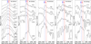 |
Fig. A.1. Detail of the spectral evolution of SNe 2020nxt, 2020taz, 2021bbv, 2023utc, and 2024aej near the expected position of the narrow interstellar Na I D absorption line (in the velocity space). v = 0 km s−1 corresponds to the rest wavelength of the core of the Na I D line. |
-
SN 2020nxt: EW ≲0.69 Å, E(B − V)host ≲ 0.09 mag
-
SN 2020taz: EW ≲0.30 Å, E(B − V)host ≲ 0.03 mag
-
SN 2021bbv: EW ≲0.40 Å, E(B − V)host ≲ 0.04 mag
-
SN 2023utc: EW ≲1.66 Å, E(B − V)host ≲ 0.26 mag
-
SN 2024aej: EW ≲1.30 Å, E(B − V)host ≲ 0.20 mag
The above upper limits to the colour excess due to the host galaxy dust attenuation are not very stringent, implying that - at least for SNe 2023utc and 2024aej - a non-negligible host galaxy extinction cannot be ruled out in principle. However, most SNe Ibn in our sample (including SNe 2023utc and 2024aej) are hosted in very faint dwarf galaxies or remote locations from the host nucleus, where large line-of-sight reddening values are not expected. Hence, while reliable estimates for E(B − V)host are not available, the position of the SNe in their host galaxies and/or their morphologic types support the choice of assuming a negligible host galaxy reddening for all objects of our sample.
Appendix B: Basic information for observational facilities used for the five SNe Ibn
We report the basic information for observational facilities in Table B.1, which were used for the five SNe Ibn.
Information on the instrumental setups.
Appendix C: Peak time of our sample of SNe Ibn
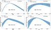 |
Fig. C.1. Peak time of SNe 2020nxt, 2020taz, 2023utc, 2024aej. |
Appendix D: Decline rates of light curves of five SNe Ibn
Decline rates of the light curves of individual SNe.
Appendix E: MOSFiT corner plots of five SNe Ibn
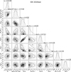 |
Fig. E.1. Corner plot showing the posterior distributions of the fitted parameters for SN 2020nxt, based on the RD+CSI model using MOSFiT. Median values are indicated by vertical lines, with the shaded regions representing the 68% confidence intervals. |
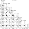 |
Fig. E.2. Corner plot showing the posterior distributions of the fitted parameters for SN 2020taz, based on the RD+CSI model using MOSFiT. Median values are indicated by vertical lines, with the shaded regions representing the 68% confidence intervals. |
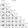 |
Fig. E.3. Corner plot showing the posterior distributions of the fitted parameters for SN 2021bbv, based on the RD+CSI model using MOSFiT. Median values are indicated by vertical lines, with the shaded regions representing the 68% confidence intervals. |
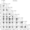 |
Fig. E.4. Corner plot showing the posterior distributions of the fitted parameters for SN 2023utc, based on the RD+CSI model using MOSFiT. Median values are indicated by vertical lines, with the shaded regions representing the 68% confidence intervals. |
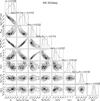 |
Fig. E.5. Corner plot showing the posterior distributions of the fitted parameters for SN 2024aej, based on the RD+CSI model using MOSFiT. Median values are indicated by vertical lines, with the shaded regions representing the 68% confidence intervals. |
Appendix F: Log of the spectroscopic observations
Log of the spectroscopic observations of SN 2020nxt.
Log of the spectroscopic observations of SN 2020taz.
Log of the spectroscopic observations of SN 2021bbv.
Log of the spectroscopic observations of SN 2023utc.
Log of the spectroscopic observations of SN 2024aej.
Appendix G: Modelling the spectra
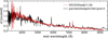 |
Fig. G.1. Comparison between the observed spectrum of SN 2020taz obtained on 29 September 2020, corresponding to 11.0 days after the estimated time of maximum light (MJD = 59121.85), and a synthetic spectrum from a CDS model based on he4p0. The model assumes a shell located at a radius of 1.5 × 1015 cm, expanding at a velocity of 500 km s−1, and powered at a rate of 3 × 1042 erg s−1. No smoothing has been applied to either the observed or synthetic spectra. The model spectra were provided by L. Dessart (priv. comm.). |
Appendix H: Acknowledgements
We gratefully thank the anonymous referee for his/her insightful
comments and suggestions that improved the paper. We thank Luc Dessart for kindly providing the light curve and spectral models for
SNe Ibn, as well as for his valuable guidance and support to this work. We are also grateful to Qinan Wang for sharing data and engaging in helpful discussions. We thank Qiliang Fang for his helpful discussions. This study is supported by the National Natural Science Foundation of China (Grant Nos. 12303054,12225304), the National Key Research and Development Program of China (Grant No. 2024YFA1611603), the Yunnan Fundamental Research Projects (Grant Nos. 202401AU070063, 202501AS070078), and the International Centre of Supernovae, Yunnan Key Laboratory (No. 202302AN360001). AP, AR, SB, EC, NER, LT, GV acknowledge support from the PRIN-INAF 2022, "Shedding light on the nature of gap transients: from the observations to the models". AR also acknowledges financial support from the GRAWITA Large Program Grant (PI P. D’Avanzo). WLL is supported by the National Natural Science Foundation of China (NSFC grants 12473045, 12033003 and 12494572) and the Natural Science Foundation of Xiamen city (grant 3502Z202471015). EC acknowledges support from MIUR, PRIN 2020 (METE, grant 2020KB33TP). N.E.R. acknowledges support from the Spanish Ministerio de Ciencia e Innovación (MCIN) and the Agencia Estatal de Investigación (AEI) 10.13039/501100011033 under the program Unidad de Excelencia María de Maeztu CEX2020-001058-M. JRF is supported by the National Science Foundation Graduate Research Fellowship Program under Grant No. (NSF 2139319). A.F. acknowledges the support by the State of Hesse within the Research Cluster ELEMENTS (Project ID 500/10.006). Shane Moran is funded by Leverhulme Trust grant RPG-2023-240. M.D. Stritzinger is funded by the Independent Research Fund Denmark (IRFD, grant number 10.46540/2032-00022B). GJW acknowledges the Africa Europe Cluster of Research Excellence (CoRE-AI) fellowship. XFW is supported by the National Natural Science Foundation of China (NSFC grants 12288102, 12033003, and 11633002) and the Tencent Xplorer Prize. CPG acknowledges financial support from the Secretary of Universities and Research (Government of Catalonia) and by the Horizon 2020 Research and Innovation Programme of the European Union under the Marie Skłodowska-Curie and the Beatriu de Pinós 2021 BP 00168 programme, from the Spanish Ministerio de Ciencia e Innovación (MCIN) and the Agencia Estatal de Investigación (AEI) 10.13039/501100011033 under the PID2023-151307NB-I00 SNNEXT project, from Centro Superior de Investigaciones Científicas (CSIC) under the PIE project 20215AT016 and the program Unidad de Excelencia María de Maeztu CEX2020-001058-M, and from the Departament de Recerca i Universitats de la Generalitat de Catalunya through the 2021-SGR-01270 grant. T.K. acknowledges support from the Research Council of Finland project 360274. Song-Peng Pei is supported by the Science and Technology Foundation of Guizhou Province (QKHJC-ZK[2023]442). T.M.R is part of the Cosmic Dawn Center (DAWN), which is funded by the Danish National Research Foundation under grant DNRF140. T.M.R acknowledges support from the Research Council of Finland project 350458. C.-Y. Wu is supported by the National Natural Science Foundation of China (NSFC, Grant No.12473032), the Yunnan Revitalization Talent Support Program–Young Talent project, and the International Centre of Supernovae, Yunnan Key Laboratory (No. 202302AN360001). J.Z. is supported by the National Key R&D Program of China with No. 2021YFA1600404, the National Natural Science Foundation of China (12173082, 12333008), the Yunnan Fundamental Research Projects (grants 202401BC070007 and 202201AT070069), the Top-notch Young Talents Program of Yunnan Province, the Light of West China Program provided by the Chinese Academy of Sciences, and the International Centre of Supernovae, Yunnan Key Laboratory (No. 202302AN360001). XJZ is supported by the National Natural Science Foundation of China (Grant No. 12203004) and by the Fundamental Research Funds for the Central Universities. We acknowledge the support of the staffs of the various observatories at which data were obtained. We thank Melissa L. Graham for providing an APO-3.5m spectrum of SN 2020taz, and Kenta Taguchi for sharing a spectrum of SN 2023utc obtained through the 3.8 m Seimei Telescope. We acknowledge the support of the staff of the Xinglong 80 cm telescope (TNT). Based on observations made with the Nordic Optical Telescope, owned in collaboration by the University of Turku and Aarhus University, and operated jointly by Aarhus University, the University of Turku, and the University of Oslo, representing Denmark, Finland, and Norway, the University of Iceland, and Stockholm University at the Observatorio del Roque de los Muchachos, La Palma, Spain, of the Instituto de Astrofisica de Canarias. Observations from the NOT were obtained through the NUTS2 collaboration which is supported in part by the Instrument Centre for Danish Astrophysics (IDA), and the Finnish Centre for Astronomy with ESO (FINCA) via Academy of Finland grant nr 306531. The data presented here were obtained in part with ALFOSC, which is provided by the Instituto de Astrofisica de Andalucia (IAA) under a joint agreement with the University of Copenhagen and NOTSA. The Liverpool Telescope is operated on the island of La Palma by Liverpool John Moores University in the Spanish Observatorio del Roque de los Muchachos of the Instituto de Astrofisica de Canarias with financial support from the UK Science and Technology Facilities Council. The Italian Telescopio Nazionale Galileo (TNG) operated on the island of La Palma by the Fundación Galileo Galilei of the INAF (Istituto Nazionale di Astrofisica) at the Spanish Observatorio del Roque de los Muchachos of the Instituto de Astrofísica de Canarias. Based on observations collected at Copernico and Schmidt telescopes (Asiago, Italy) of the INAF – Osservatorio Astronomico di Padova. Based on observations obtained with the Gran Telescopio Canarias (GTC), installed in the Spanish Observatorio del Roque de los Muchachos of the Instituto de Astrofisica de Canarias, on the island of La Palma. Based on data products from observations made with ESO Telescopes at the La Silla Paranal Observatory under programmes 106.216C.004/010 (D/J): ePESSTO+ (the advanced Public ESO Spectroscopic Survey for Transient Objects). This work has made use of data from the Asteroid Terrestrial-impact Last Alert System (ATLAS) project. The Asteroid Terrestrial-impact Last Alert System (ATLAS) project is primarily funded to search for near earth asteroids through NASA grants NN12AR55G, 80NSSC18K0284, and 80NSSC18K1575; byproducts of the NEO search include images and catalogs from the survey area. This work was partially funded by Kepler/K2 grant J1944/80NSSC19K0112 and HST GO-15889, and STFC grants ST/T000198/1 and ST/S006109/1. The ATLAS science products have been made possible through the contributions of the University of Hawaii Institute for Astronomy, the Queen’s University Belfast, the Space Telescope Science Institute, the South African Astronomical Observatory, and The Millennium Institute of Astrophysics (MAS), Chile. This work makes use of data from the Las Cumbres Observatory Network and the Global Supernova Project. The LCO team is supported by U.S. NSF grants AST-1911225 and AST-1911151, and NASA. We thank Las Cumbres Observatory and its staff for their continued support of ASAS-SN. ASAS-SN is funded in part by the Gordon and Betty Moore Foundation through grants GBMF5490 and GBMF10501 to the Ohio State University, and also funded in part by the Alfred P. Sloan Foundation grant G-2021-14192. Development of ASAS-SN has been supported by NSF grant AST-0908816, the Mt. Cuba Astronomical Foundation, the Center for Cosmology and AstroParticle Physics at the Ohio State University, the Chinese Academy of Sciences South America Center for Astronomy (CAS-SACA), and the Villum Foundation. Pan-STARRS is a project of the Institute for Astronomy of the University of Hawaii, and is supported by the NASA SSO Near Earth Observation Program under grants 80NSSC18K0971, NNX14AM74G, NNX12AR65G, NNX13AQ47G, NNX08AR22G, 80NSSC21K1572 and by the State of Hawaii. The Pan-STARRS1 Surveys (PS1) and the PS1 public science archive have been made possible through contributions by the Institute for Astronomy, the University of Hawaii, the Pan-STARRS Project Office, the Max-Planck Society and its participating institutes, the Max Planck Institute for Astronomy, Heidelberg and the Max Planck Institute for Extraterrestrial Physics, Garching, The Johns Hopkins University, Durham University, the University of Edinburgh, the Queen’s University Belfast, the Harvard-Smithsonian Center for Astrophysics, the Las Cumbres Observatory Global Telescope Network Incorporated, the National Central University of Taiwan, STScI, NASA under grant NNX08AR22G issued through the Planetary Science Division of the NASA Science Mission Directorate, NSF grant AST-1238877, the University of Maryland, Eotvos Lorand University (ELTE), the Los Alamos National Laboratory, and the Gordon and Betty Moore Foundation. The Zwicky Transient Facility (ZTF) is supported by the National Science Foundation under Grants No. AST-1440341 and AST-2034437 and involves a collaboration that includes current partners such as Caltech, IPAC, the Oskar Klein Center at Stockholm University, the University of Maryland, the University of California, Berkeley, the University of Wisconsin-Milwaukee, the University of Warwick, Ruhr University, Cornell University, Northwestern University, and Drexel University. Operations are conducted by COO, IPAC, and UW. We acknowledge the use of public data from the Swift data archive. SDSS is managed by the Astrophysical Research Consortium for the Participating Institutions of the SDSS Collaboration including the Brazilian Participation Group, the Carnegie Institution for Science, Carnegie Mellon University, Center for Astrophysics | Harvard & Smithsonian (CfA), the Chilean Participation Group, the French Participation Group, Instituto de Astrofísica de Canarias, The Johns Hopkins University, Kavli Institute for the Physics and Mathematics of the Universe (IPMU) / University of Tokyo, the Korean Participation Group, Lawrence Berkeley National Laboratory, Leibniz Institut für Astrophysik Potsdam (AIP), Max-Planck-Institut für Astronomie (MPIA Heidelberg), Max-Planck-Institut für Astrophysik (MPA Garching), Max-Planck-Institut für Extraterrestrische Physik (MPE), National Astronomical Observatories of China, New Mexico State University, New York University, University of Notre Dame, Observatório Nacional / MCTI, The Ohio State University, Pennsylvania State University, Shanghai Astronomical Observatory, United Kingdom Participation Group, Universidad Nacional Autónoma de México, University of Arizona, University of Colorado Boulder, University of Oxford, University of Portsmouth, University of Utah, University of Virginia, University of Washington, University of Wisconsin, Vanderbilt University, and Yale University. This research has made use of the NASA/IPAC Extragalactic Database (NED), which is operated by the Jet Propulsion Laboratory, California Institute of Technology, under contract with the National Aeronautics and Space Administration. IRAF was distributed by the National Optical Astronomy Observatory, which was managed by the Association of Universities for Research in Astronomy (AURA), Inc., under a cooperative agreement with the U.S. NSF.
All Tables
All Figures
|
Fig. 1. SN 2020nxt in a NOT/ALFOSC image taken with a Sloan i-band filter on 19 July 2020; SN 2020taz in a NOT/ALFOSC image taken with a Sloan r-band filter on 1 October 2020; SN 2021bbv in a NOT/ALFOSC image taken with a Sloan i-band filter on 17 February 2021; SN 2023utc in a LCO TFN/fa20 image taken with a Sloan i-band filter on 27 October 2023; SN 2024aej in a LCO TFN/fa11 image taken with a Sloan r-band filter on 17 January 2024. |
| In the text | |
|
Fig. 2. Ultraviolet and optical light curves of SNe 2020nxt, 2020taz, 2021bbv, 2023utc, and 2024aej. The dashed vertical line marks the o/r-band maximum light as the reference epoch. The epochs of our spectra are marked with vertical solid red lines on the top. The upper limits are marked by empty symbols with arrows. For clarity, the light curves for the different bands are shifted with arbitrary constants as reported in the legend. Usually, magnitude errors are smaller than the symbols. |
| In the text | |
|
Fig. 3. Constraints on the explosion epochs of SNe 2020taz (left) and 2024aej (right). Early time ATLAS o-filter data are shown in the flux space. The zero flux level is marked by a horizontal dashed line. Red dots indicate real detections, while blue circles show the latest detection limit. |
| In the text | |
|
Fig. 4. Colour evolution of SNe 2020nxt, 2020nxt, 2021bbv, 2023utc, and 2024aej compared with a large sample of SNe Ibn from the literature. The colour curves have been corrected for Galactic extinction. |
| In the text | |
|
Fig. 5. Light curves of SNe 2020nxt, 2020taz, 2021bbv, 2023utc, and 2024aej in the R/r-band including the comparison SNe Ibn. The template r-band light curves for SNe Ibn are from Hosseinzadeh et al. (2017, yellow) and Khakpash et al. (2024, purple). |
| In the text | |
|
Fig. 6. Pseudo-bolometric light curves of SNe 2020nxt, 2020taz, 2021bbv, 2023utc, and 2024aej compared with those of a sample of SNe Ibn. |
| In the text | |
|
Fig. 7. Representative blackbody fits to the SEDs at epochs near the peak luminosity for each SN in our sample. The blue lines show the best-fitting blackbody functions. For visual clarity, the SEDs have been vertically offset by arbitrary constants. |
| In the text | |
|
Fig. 8. Evolution of the blackbody temperature and radius for our SN sample. |
| In the text | |
|
Fig. 9. Comparison between the bolometric light curves of the five SNe Ibn in our sample and representative interaction models from Dessart et al. (2022). The left panel displays simulations involving ejecta–wind interactions, while the right panel shows ejecta–ejecta interaction scenarios. |
| In the text | |
|
Fig. 10. Light curves from the RD+CSI model fitted to the multi-band photometry of five SNe Ibn using the Monte Carlo code MOSFiT. For each filter, a representative subset of model light curves randomly drawn from the posterior distributions is shown to illustrate the range of the model fits. The latest pre-discovery upper limits are indicated by triangles. |
| In the text | |
|
Fig. 11. Relationships between parameters inferred from the light curves of SNe Ibn. Top left: R/r-band peak magnitude versus rise time. Top right: R/r-band peak magnitude versus R/r-band decline rate. Centre left: Rise time versus R/r-band decline rate. Centre right: Peak luminosity (Lpeak) versus t0.5 (the time required for the luminosity to decline by half from its peak). Bottom left: Kinetic energy (EK) versus synthesised 56Ni mass. The weighted Pearson correlation coefficient (rP), the Spearman rank correlation coefficient (rS), and the associated p-values (probability of chance correlation) are provided for each parameter pair. Statistics exclude data points with rise time and peak magnitude limits. |
| In the text | |
|
Fig. 12. Spectral sequences of the five SNe Ibn. The dashed vertical lines indicate the main H and He I transitions, while the ⊕ symbol marks the strongest telluric absorption bands. All spectra have been corrected for redshift and extinction. Grey lines represent smoothed spectra (originally with a lower S/N) processed with a Savitzky-Golay filter. |
| In the text | |
|
Fig. 13. Line identification in the highest-resolution late-time spectra of the five SNe presented in this paper. Spectra have been corrected for redshift and reddening, with indicated phases from the maximum light. |
| In the text | |
|
Fig. 14. Comparison of around-peak (purple) and late-time (green) spectra of SNe 2020nxt, 2020taz, 2021bbv, 2023utc, and 2024aej with other SNe Ibn at similar phases. All spectra have been corrected for redshift and extinction. Significant He I features are marked by blue dashed lines, while Balmer features by red dashed lines. |
| In the text | |
|
Fig. 15. Evolution of He I line velocities. Left panel: Temporal evolution of the velocities associated with the narrow He I line components, which trace the unshocked CSM. Right panel: Velocity evolution of the broader He I emission components, reflecting the dynamics of the shocked gas region. Data for comparison SNe Ibn are adopted from Pastorello et al. (2016) and Wang et al. (2024a). |
| In the text | |
|
Fig. 16. Comparison between synthetic spectra from model he4p0 and observed spectra of five SNe Ibn at multiple epochs after bolometric maximum light. No smoothing has been applied to either the observed or modelled spectra. The synthetic spectra are based on simulations from Dessart et al. (2022) and Wang et al. (2024b) as well as newly computed models incorporating updated parameters. |
| In the text | |
|
Fig. A.1. Detail of the spectral evolution of SNe 2020nxt, 2020taz, 2021bbv, 2023utc, and 2024aej near the expected position of the narrow interstellar Na I D absorption line (in the velocity space). v = 0 km s−1 corresponds to the rest wavelength of the core of the Na I D line. |
| In the text | |
|
Fig. C.1. Peak time of SNe 2020nxt, 2020taz, 2023utc, 2024aej. |
| In the text | |
|
Fig. E.1. Corner plot showing the posterior distributions of the fitted parameters for SN 2020nxt, based on the RD+CSI model using MOSFiT. Median values are indicated by vertical lines, with the shaded regions representing the 68% confidence intervals. |
| In the text | |
|
Fig. E.2. Corner plot showing the posterior distributions of the fitted parameters for SN 2020taz, based on the RD+CSI model using MOSFiT. Median values are indicated by vertical lines, with the shaded regions representing the 68% confidence intervals. |
| In the text | |
|
Fig. E.3. Corner plot showing the posterior distributions of the fitted parameters for SN 2021bbv, based on the RD+CSI model using MOSFiT. Median values are indicated by vertical lines, with the shaded regions representing the 68% confidence intervals. |
| In the text | |
|
Fig. E.4. Corner plot showing the posterior distributions of the fitted parameters for SN 2023utc, based on the RD+CSI model using MOSFiT. Median values are indicated by vertical lines, with the shaded regions representing the 68% confidence intervals. |
| In the text | |
|
Fig. E.5. Corner plot showing the posterior distributions of the fitted parameters for SN 2024aej, based on the RD+CSI model using MOSFiT. Median values are indicated by vertical lines, with the shaded regions representing the 68% confidence intervals. |
| In the text | |
|
Fig. G.1. Comparison between the observed spectrum of SN 2020taz obtained on 29 September 2020, corresponding to 11.0 days after the estimated time of maximum light (MJD = 59121.85), and a synthetic spectrum from a CDS model based on he4p0. The model assumes a shell located at a radius of 1.5 × 1015 cm, expanding at a velocity of 500 km s−1, and powered at a rate of 3 × 1042 erg s−1. No smoothing has been applied to either the observed or synthetic spectra. The model spectra were provided by L. Dessart (priv. comm.). |
| In the text | |
Current usage metrics show cumulative count of Article Views (full-text article views including HTML views, PDF and ePub downloads, according to the available data) and Abstracts Views on Vision4Press platform.
Data correspond to usage on the plateform after 2015. The current usage metrics is available 48-96 hours after online publication and is updated daily on week days.
Initial download of the metrics may take a while.