| Issue |
A&A
Volume 700, August 2025
|
|
|---|---|---|
| Article Number | A155 | |
| Number of page(s) | 27 | |
| Section | Interstellar and circumstellar matter | |
| DOI | https://doi.org/10.1051/0004-6361/202554879 | |
| Published online | 14 August 2025 | |
Nickel- and iron-rich clumps in planetary nebulae: New discoveries and emission-line diagnostics
1
Institute for Astronomy, Astrophysics, Space Applications and Remote Sensing, National Observatory of Athens,
15236
Penteli,
Greece
2
Department of Physics, University of Patras,
Patras,
26504
Rio,
Greece
3
School of Physics and Astronomy, Cardiff University, Queen’s Buildings, The Parade,
Cardiff CF24 3AA,
UK
4
Instituto de Física e Química, Universidade Federal de Itajuba,
Av. BPS 1303-Pinheirinho,
37500-903,
Ítajuba,
Brazil
5
Instituto de Astrofísica de Canarias,
38205 La Laguna,
Tenerife,
Spain
6
Departamento de Astrofísica, Universidad de La Laguna,
E-38206 La Laguna,
Tenerife,
Spain
7
Observatório do Valongo, Universidade Federal do Rio de Janeiro,
Ladeira Pedro Antonio 43,
20080-090
Rio de Janeiro,
Brazil
8
Laboratório Nacional de Astrofísica, Rua dos Estados Unidos,
154, Bairro das Nações,
Itajubá,
MG
37504-365,
Brazil
9
Leiden Observatory, Leiden University,
PO Box 9513,
2300
RA Leiden,
The Netherlands
10
Department of Physics and Astronomy, University of Western Ontario,
London,
ON
N6A 3K7,
Canada
11
Institute for Earth and Space Exploration, University of Western Ontario,
London,
ON
N6A 3K7,
Canada
12
SETI Institute,
189 Bernardo Ave, Suite 100,
Mountain View,
CA
94043,
USA
★ Corresponding authors: This email address is being protected from spambots. You need JavaScript enabled to view it.
; This email address is being protected from spambots. You need JavaScript enabled to view it.
Received:
31
March
2025
Accepted:
12
June
2025
Abstract
Context. Integral field spectroscopy (IFS) offers a distinct advantage for studying extended sources by enabling spatially resolved emission maps for several emission lines without the need for specific filters.
Aims. This study aims to conduct a detailed analysis of iron and nickel emission lines in 12 planetary nebulae (PNe) using integral field unit (IFU) data from MUSE to provide valuable insights into their formation and evolution mechanisms.
Methods. New diagnostic line ratios, combined with machine-learning algorithms, were used to distinguish excitation mechanisms such as shock and photoionization. Electron densities and elemental abundances were estimated for different atomic data using the PYNEB package. The contribution of fluorescent excitation of nickel lines was also examined.
Results. A total of 16 iron- and nickel-rich clumps are detected in seven out of 12 PNe. New clumps are discovered in NGC 3132 and IC 4406. The most prominent lines are [Fe II] 8617 Å and [Ni II] 7378 Å. Both emission lines are observed emanating directly from the low-ionization structures (LIS) of NGC 3242, NGC 7009, and NGC 6153, as well as from clumps in NGC 6369 and Tc 1. Their abundances are found to be below the solar values, indicating that a fraction of Fe and Ni remains depleted in dust grains. The depletion factors exhibit a strong correlation over a wide range of values. A machine-learning approach allows us to classify ten out of 16 clumps as shock-excited and to establish a new shock/photoionization selection criterion: log ([Ni II] 7378 Å/Hα) & log ([Fe II] 8617 Å/Hα) > −2.20.
Key words: atomic data / shock waves / techniques: imaging spectroscopy / ISM: abundances / dust, extinction / planetary nebulae: general
© The Authors 2025
 Open Access article, published by EDP Sciences, under the terms of the Creative Commons Attribution License (https://creativecommons.org/licenses/by/4.0), which permits unrestricted use, distribution, and reproduction in any medium, provided the original work is properly cited.
This article is published in open access under the Subscribe to Open model. This email address is being protected from spambots. You need JavaScript enabled to view it. to support open access publication.
1 Introduction
The powerful technique of integral field spectroscopy (IFS) has revolutionized the way we study extended astronomical objects. Integral field units (IFUs) were initially employed in the late 1980s with TIGER/CFHT (Courtes et al. 1988), and since then numerous instruments have been developed. Most IFUs included in planetary nebula (PN) studies are FLAMES/VLT (Pasquini et al. 2002), VIMOS/VLT (Le Fèvre et al. 2003), SINFONI/VLT (Eisenhauer et al. 2003), MUSE/VLT (Bacon et al. 2010), MEGARA/GTC (Gil de Paz et al. 2018), NIRSPEC/JWST (Böker et al. 2022), and MIRI/JWST (Argyriou et al. 2023). The wavelength coverage of most IFUs spans from near ultraviolet (NUV) to infrared (IR) wavelengths, while the field of view varies from a few arcseconds to nearly one arcminute.
Unlike previous imaging studies limited by the available filters, IFUs offer an unprecedented ability to spatially resolve emission lines from a wide range of species with different ionization states. Before the advent of IFS, knowledge of the emission region was mostly constrained by the slit position in spectroscopic studies.
A wide variety of astronomical objects have been studied using IFUs, including galaxies, active galactic nuclei (AGNs), supernova remnants (SNRs), H II regions, young stellar objects (YSOs), Herbig-Haro (HH) objects, and PNe, among others. Regarding PNe, which are the main focus of this work, IFU observations have provided unprecedented findings and novel insights into their physical and chemical properties, revealing details about ionization structures, abundance variations, and dynamical features. Several studies have demonstrated the significant advantage of imaging spectroscopy over traditional long-slit spectroscopy in the study of extended PNe (e.g., Matsuura et al. 2007; Tsamis et al. 2008; Ali et al. 2015; Ali & Dopita 2017; Dopita et al. 2017; Walsh et al. 2018; Monreal-Ibero & Walsh 2020; Rechy-García et al. 2020; Akras et al. 2022). However, the majority of the studies are focused on the brightest and more common emission lines. Notable exceptions are the studies by García-Rojas et al. (2022), Akras et al. (2024b), Gómez-Llanos et al. (2024), and Konstantinou et al. (2025), which have investigated a broader range of emission lines in PNe, including the first spatial distribution of the near-IR emission line of atomic carbon [C I] 8727 Å in low-ionization structures (LISs; Gonçalves et al. 2001; Akras & Gonçalves 2016; Mari et al. 2023b). This motivated us to look into the available MUSE data of PNe for less common and generally faint emission lines such as [Ni II] 7378 Å and [Fe II] 8617 Å.
Planetary nebulae are formed by the interaction of the slow asymptotic giant branch (AGB) wind and the fast post-AGB wind (e.g., Kwok et al. 1978; Balick 1987; Icke 1988). The nebular gas is ionized by the ultraviolet (UV) photons of the hot central star, and its spectrum is characterized by discrete emission lines (recombination or collisionally excited). Although PNe constitute only a small fraction of the lifetime of low-mass stars (∼ 104 yr) between AGB and white-dwarf phases, they play a key role in the chemical enhancement of the interstellar medium. The most common elements observed in PNe are H, He, N, S, O, Cl, Ar, C, and Ne; and in rarer cases Fe, Ni, Ca, P, Mg, K, Cr, Mn, Se, Kr, and Xe (e.g., García-Rojas et al. 2015; Sterling et al. 2017). Exploring and analyzing a wide variety of elements in PNe provides further insights into the stellar evolution of low-mass stars, both single and in binary systems.
Iron and nickel lines have been detected in a wide variety of gaseous nebulae, indicating a close correlation between them. More specifically, [Ni II] 7412 Å, 7378 Å, and 11910 Å; and [Fe II] 5158 Å, 5262 Å, 7155 Å, 8617 Å, 12570 Å, and 16440 Å emission lines appear strong in SNRs (Dennefeld 1986; Jerkstrand et al. 2015b; Temim et al. 2024), HH objects (Brugel et al. 1981; Mesa-Delgado et al. 2009; Reiter et al. 2019), and Seyfert galaxies (Halpern & Oke 1986; Henry & Fesen 1988), but they are fainter in H II regions (Osterbrock et al. 1990; Delgado-Inglada et al. 2016), circumstellar nebulae of luminous blue variables (Barlow et al. 1994; Meaburn et al. 2000), and PNe (García-Rojas et al. 2013; Delgado-Inglada & Rodríguez 2014). Table 1 lists the PNe where optical forbidden emission lines of singly ionized nickel and/or iron have been detected from previous long-slit or IFU observations.
In SNRs and some HH objects, nickel and iron emission lines are usually detected in regions influenced by shocks. In particular, high [Fe II] 1.257 μm/P α and [Fe II] 1.644 μm/Brγ line ratios are considered reliable shock tracers (Graham et al. 1987; Temim et al. 2024), whereas low values are attributed to UV radiation (e.g., Akras et al. 2024a, and references therein).
Neutral and singly ionized Fe and Ni have comparable ionization potentials (7.9 eV for Fe0, 7.6 eV for Ni0, and 16.2 eV for Fe+, 18.2 eV for Ni+), indicating that they coexist in partially ionized zones (PIZs). Fe+and Ni+are sustained in these regions because their ionization potentials are higher than H I (13.6 eV), which acts as a shield. The most prominent and brightest [Ni II] and [Fe II] emission lines are centered at 7378 Å and 8617 Å, respectively. [Ni II] 7378 Å originates from 2D5/2−2 F7/2 transition, while [Fe II] 8617 Å from the 4F9/2−4 P5/2 transition. The [Fe II] and [Ni II] lines have critical electron densities above 106 cm−3 and their excitation energies are very close: Δ E([Fe II] 8617 Å) = 1.67 eV and Δ E([Ni II] 7378 Å) = 1.68 eV (Bautista et al. 1996).
This study focuses on the first detection of nickel and iron emissions from clumps embedded in PNe. Sect. 2 describes the PNe sample and their properties, while Sect. 3 provides details of the conducted spectroscopic analysis. Sect. 4 presents the main findings of our study, and Sect. 5 outlines our machine-learning approach to interpreting the results and estimating additional physical parameters (e.g., density, abundances, depletion factors). Finally, Sect. 6 discusses the origin of Fe and Ni in PNe, and Sect. 7 summarizes the conclusions of our study.
PNe where optical forbidden emissions of [Ni II] and/or [Fe II] were detected.
PNe with available MUSE data in the ESO archive used in this work.
2 ESO archival data and sample description
We gathered most of the available and already reduced MUSE data of PNe from the ESO archive, where the standard data-reduction process was carried out using ESO pipelines1 (a summary of reduction steps can be found in Sect. 2 of García-Rojas et al. 2022). Table 2 presents the list of PNe in our study with information on their observations.
Multi Unit Spectroscopic Explorer (MUSE; Bacon et al. 2010) is an IFU mounted on the UT4 of the Very Large Telescope (VLT) in Cerro Paranal, Chile. The wide field mode (WFM) of MUSE provides a field of view of 1′ × 1′ and spatial resolution of 0.2′′ per pixel, while the wavelength range spans from 4800 Å to 9300 Å in the nominal spectral mode and from 4600 Å to 9300 Å in the extended spectral mode. The resolving power is 1770 at the blue part of the spectrum and 3590 at the red part. The outcome from an IFU, such as MUSE, is a data cube with two spatial dimensions and a spectral one.
NGC 3242 is a multiple-shell PN with a bright rim and a pair of symmetric LISs. It is ionized by an O-type star with a spectral type O(H) (Weidmann et al. 2020, and references therein), Teff = 80 000 K, and log (L/L⊙) = 2.86 (Pottasch & Bernard-Salas 2008). A triple central system has also been proposed for this nebula (Soker et al. 1992). Moreover, NGC 3242 has been detected in X-ray emission with XMM-Newton (Ruiz et al. 2011).
NGC 6153 is a 3.2 kyr (González-Santamaría et al. 2021) elliptical nebula with two bright regions at the end of its minor axis and several smaller clumps. A weak-emission-line star (wels) is present at the center with Teff = 110 000 K and log (L/L⊙) = 3.76 (González-Santamaría et al. 2021). There is probably an unseen stellar companion, as recent Gaia measurements indicate (Chornay et al. 2021). Also, the abundance discrepancy factor (ADF) of the nebula was found to be high (Liu et al. 2000; Gómez-Llanos et al. 2024), which is probably due to the presence of a binary system (see Sect. 5.1).
Hf 2-2 is a spherical nebula with a bright and fragmented ring seen in [N II] images. A short-orbital-period (∼ 0.4 days) post-common-envelope binary system has been found at the center of this nebula (Lutz et al. 1998; Bond 2000). Furthermore, it is characterized by high ADF (Liu et al. 2006; García-Rojas et al. 2022), and its central star has an O(H) 3 spectral type (Weidmann et al. 2020).
M 1-42 is an elliptical nebula with symmetrical clumps alongside its major axis. In addition, a high ADF has been derived for this nebula (Liu et al. 2001; García-Rojas et al. 2022), probably indicating the presence of a binary system.
NGC 6778 is a 4.4 kyr (Tocknell et al. 2014) irregular nebula with jet-like structures. NGC 6778 hosts a close binary central star that has undergone a common-envelope phase with short orbital period (∼ 0.15 days, Miszalski et al. 2011), which is consistent with the high ADF measured in this nebula (Jones et al. 2016; García-Rojas et al. 2022).
NGC 7009 is a 1.9 kyr (González-Santamaría et al. 2021) elliptical nebula with two pairs of LISs located along its major axis. H2 emission was recently detected in the outer pair of LISs (Akras et al. 2020a). The central star of the PN (CSPN) is an O(H) spectral-type star with Teff = 82 000 K and log (L/L⊙) = 3.97 (Mendez et al. 1992).
NGC 3132 is a young, elliptical, and molecule-rich PN (Kastner et al. 2024), likely with a multi-stellar system (De Marco et al. 2022). The CS has Teff = 100 000 K, log (L/L⊙) = 2.19 (Frew 2008), and an A2V spectral type (Weidmann et al. 2020).
IC 418 is a 1.6 kyr (Weidmann et al. 2020, and references therein) spherical nebula with a CSPN of Teff = 38 000 K, log (L/L⊙) = 3.77, and the spectral type O7fp. Moreover, emission from polycyclic aromatic hydrocarbons (PAHs) at 13.2 μm and fullerenes at 17.4 μm have been detected in this nebula (Díaz-Luis et al. 2018).
NGC 6369 has a complex morphology with a bright and fragmented rim. Its central star is an oxygen-rich Wolf-Rayet star with a spectral type of [WO 3] (Weidmann et al. 2020, and references therein), Teff = 70 000 K, and \log (L/L⊙) = 3.38 (Pottasch & Bernard-Salas 2008). The presence of a stellar companion has also been proposed based on the Gaia measurements (Chornay et al. 2021). Molecular hydrogen and PAHs have also been identified in this nebula (Ramos-Larios et al. 2012).
NGC 6563 is a 6.35 kyr elliptical nebula. Its central star is characterized by Teff = 123 000 K and log (L/L⊙) = 1.84, and its progenitor mass was estimated ∼ 2.9 M⊙ (González-Santamaría et al. 2021).
IC 4406 has a prolate spheroid shape, and its CSPN has been classified as a Wolf-Rayet star [WR] (Weidmann et al. 2020, and references therein). Recent Gaia measurements suggest the existence of a binary system at the center of the nebula (Chornay et al. 2021). Moreover, CO and H2 emission have been found alongside the nebula’s major axis (Sahai et al. 1991; Ramos-Larios et al. 2022).
Tc 1 is a young, slightly elongated spheroid and fullerenerich nebula (Cami et al. 2010) with a spectacular round halo. Its central star has a spectral type of O(H) 5–9 f (Weidmann et al. 2020, and references therein) with 30 000 K < Teff < 34 000 K and 3.3 < log (L/L⊙) < 3.6 (Otsuka et al. 2014; Aleman et al. 2019). In addition, Ali & Mindil (2023) identified the CS of Tc 1 as a variable star, based on GAIA DR3 data, linking it to a possible binary system.
Emission lines detected from the MUSE data in our sample of PNe.
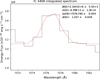 |
Fig. 1 Fitting procedure of [Ni II] 7378 Å in IC 4406 data cube. The black line represents the observation and the red line shows the Gaussian fitting of the emission line. |
3 Spectroscopic analysis
3.1 Emission-line extraction
Each MUSE data cube underwent a careful inspection for the detection of Fe and Ni along with C and Ca faint emission lines. We searched the available literature to identify the strongest emission lines within the MUSE wavelength range from 4650 Å to 9300 Å for these elements, as indicated in Table 3. Emission lines were extracted from the data cubes by fitting a Gaussian profile and subtracting the continuum emission using a Python code. The code is capable of simultaneously fitting multiple distributions and gives both the emission-line maps and the corresponding error maps as output. Fig. 1 displays, as an illustrative example, the fitting of the [Ni II] 7378 Å emission line in the data cube of IC 4406.
Given that the optical iron and nickel lines are nearly two or three orders of magnitude fainter than Hβ, we employed three steps to assure their detection. Emission lines were extracted from both the original data cube from binned versions (2 × 2 or 3 × 3), where adjacent pixel values are combined to enhance sensitivity at the expense of reducing the spatial resolution. While binning increases signal-to-noise ratio, it can introduce uncertainties when applied to regions with spatially varying nebular backgrounds. This is why we used binned data solely to verify the detection in the original cube; all flux measurements presented in this study were derived exclusively from the original data cubes. Furthermore, we cross-checked the literature for potential emission lines or skylines close to the wavelengths of interest. In most cases2, no strong emission lines were found nearby, allowing us to rule out the contribution of other elements and possible misidentification. Moreover, we compared the resulting emission-line maps with their corresponding error maps, which were generated during the fitting procedure. These errors include uncertainties from the instruments, the observational errors, and possible systematics from blending with nearby lines and sky substraction residuals. To ensure the reliability of our findings, we established a criterion requiring the flux-to-error ratio > 3 for each pixel in the extracted emission-line maps. Lastly, spectra in the wavelength range of 7350–7400 Å and 8550–8750 Å were extracted for several regions in order to visually support our detections. The spectra are presented in Appendix B, where [Fe II] 8617 Å and [Ni II] 7378 Å are indicated with vertical orange and blue lines, respectively.
3.2 Flux measurements
Besides the extraction of the spectra, we computed the fluxes of the Hα, Hβ, Paschen 10 (P10: 9015 Å), [O I] 6300 Å, [Fe II] 8617 Å, and [Ni II] 7378 Å emission lines. The first three were used to compute the extinction coefficient (c(Hβ))3 using the PYNEB 1.1.19 package (Luridiana et al. 2015; Morisset et al. 2020) and correct the fluxes for interstellar extinction (see Table 4). As a proof of concept, the extinction coefficient in NGC 3132 was estimated from both Hα/Hβ and P 10/Hβ ratios, with differences of only ∼ 5% when using the integrated values over the whole nebula.
The selected regions, where line fluxes were measured, are constrained by the [Ni II] 7378 Å line, since it is the weakest. The regions are displayed on the [O I] 6300 Å emission map of each PN in Appendix A. Our Hβ and [O I] fluxes as well the interstellar extinction are, within errors, in agreement with previous studies (NGC 3242, c(Hβ) = 0.14 Konstantinou et al. (2025); NGC 6153, c(Hβ) = 1.2 Gómez-Llanos et al. (2024); NGC 7009, c(Hβ) = 0.12 Walsh et al. (2018); Akras et al. (2022); NGC 3132, c(Hβ) = 0.14 Monreal-Ibero & Walsh (2020); NGC 6369, c(Hβ) = 2.12 Pottasch & Bernard-Salas (2008); IC 4409, c(Hβ) = 0.27 Corradi et al. (1997); Tc 1, c(Hβ) ranges from 0.28-0.44 Frew et al. (2013); Aleman et al. (2019)). This assures that our process for calculating the emission-line fluxes is reliable.
Emission-line intensities normalized to Hβ = 100 for the clump regions in our sample of PNe.
4 Results
4.1 NGC 3242
The NW and SE LISs of NGC 3242 are well known and studied (e.g., Pottasch & Bernard-Salas 2008; Monteiro et al. 2013). However, these studies focused primarily on the most prominent emission lines, except Konstantinou et al. (2025), which was the first to pay attention to the faint [C I] emission. In this work, we focused on the detection of the emission lines from heavier element lines, such as [Fe III] 4881 Å and 5270 Å, [Fe II] 7155 Å, and 8617 Å and [Ni II] 7378 Å (Figs. 2 and A.1) (some were already mentioned in Konstantinou et al. 2025). The [Fe II] and [Ni II] emission lines clearly emanate from the LISs of NGC 3242 (k1 and k4 features in Gómez-Muñoz et al. 2015).
Further analysis has revealed an intriguing spatial offset between [Fe II] 8617 Å and [C I] 8727 Å, which is of ∼ 0.5′′ for the NW LIS and ∼ 1′′ for the SE LIS (Fig. 3). More specifically, [Fe II] emission peaks at larger radial distances from the central star compared to the [C I] line. A similar behavior is observed for the [Ni II] 7378 Å line, but with higher uncertainties. This offset could likely reflect the ionization gradient, different shock fronts, or even possible differences in dust absorption. On the other hand, [Fe III] 5270 Å emission shows a jet-like structure, which is probably associated with the LISs and was also noted by Konstantinou et al. (2025). The excitation mechanisms of the [Fe II], [Fe III], and [Ni II] lines observed in this nebula are discussed in Sect. 4.
4.2 NGC 6153
NGC 6153 displays two prominent LISs at the eastern and western parts of the nebula, as illustrated by the [O I] 6300 Å line map (Fig. A.2). We verified the detection of the emission lines [Fe III] 4881 Å and 5270 Å, [Fe II] 7155 Å and 8617 Å, and [Ni II] 7378 Å and [C I] 8727 Å (Fig. 4). [Fe II] 8617 Å and [Ni II] 7378 Å lines are found to emanate from the same regions, while [Fe III] 5270 Å comes from two district regions with different orientation.
4.3 Hf 2-2
Hf 2-2 shows a spherical shell that is highly fragmented into knots, which are prominent in low-ionization lines (e.g., [O I] 6300 Å). Neither Fe nor Ni emission lines were detected in this PN (Fig. A.3).
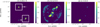 |
Fig. 2 NGC 3242 emission-line maps of [Fe II] 8617 Å, [Fe III] 5270 Å, and [Ni II] 7378 Å. White boxes represent zoomed-in views of smoothed and higher contrast versions of the selected regions. [Ni II] and [Fe III] emission-line maps are smoothed and scaled down 3 times from the original. Color-bar values are in units of 10−20 erg s−1 cm−2. |
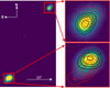 |
Fig. 3 NGC 3242 [O I] 6300 Å emission map with [C I] 8727 Å (black) and [Fe II] 8617 Å (red) line contours overlaid. |
4.4 M 1-42
M 1-42 is characterized by an ellipsoidal shell and five LISs along the major axis of the nebula, which are likely associated with a jet-like structure (Guerrero et al. 2013). The LISs were only detected in the typical low-ionization lines, such as [N II] 6548 Å and 6584 Å, [S II] 6716 Å, and 6731 Å and [O I] 6300 Å (numbers 1 to 5 in Fig. A.5). The [C I] 8727 Å emission line was successfully identified at the western and eastern edges of the nebula. No Fe or Ni lines were detected in this nebula either.
4.5 NGC 6778
NGC 6778 was recently examined by Akras et al. (2022) and García-Rojas et al. (2022). The [C I] 8727 Å originates from the inner filamentary structure, alongside neutral oxygen 6300 Å (see Fig. A.4). There is an indication (very low signal-to-noise ratio) of [Ni II 7378 Å emission; thus, further investigation is required to confirm its possible detection.
4.6 NGC 7009
The Saturn nebula is one of the most studied PNe in the literature (e.g., Gonçalves et al. 2003; Walsh et al. 2018), Akras et al. 2022, 2024b). It is characterized by an inner ellipsoidal structure and two pairs of LISs. Recently, molecular hydrogen emission was detected in the outer LISs (Akras et al. 2020a), alongside the [C I] 8727 Å and [Fe II] 1.644 μm emission lines (Akras et al. 2024a, b). By scrutinizing the MUSE data cube, we can also report the detection of doubly ionized iron lines ([Fe III] 4658 Å, 4701 Å, 4881 Å, and 5270 Å) and singly ionized iron and nickel lines ([Fe II] 5158 Å, 7155 Å, 8617 Å, and [Ni II] 7378 Å) (Figs. 5 and A.6). Some of these lines were previously detected in the deep, long-slit spectra from Fang & Liu (2011); however, the slit did not cover the outer pair of LISs. The MUSE IFU data have revealed that the [Fe II] and [Ni II] lines emanate from both the inner and outer pair of LISs (K1 to K 4, Gonçalves et al. 2003), while [Fe III] is detected only from the inner LISs (K2 and K3) (see Fig. 5).
Similarly to the case of NGC 3242, a spatial offset between the [Fe II] 8617 Å and [C I] 8727 Å lines have been found in the outer pair of LIS as well as the northern clump. In particular, the peak of [Fe II] 8617 Å is located 0.4′′ closer to the central star in the E LIS (K1), and 0.5′′ further away in the northern clump (see Fig. 6). As mentioned in Sect. 4.1, additional observations are needed in order to clarify whether ionization stratification or dynamical effects are responsible for this offset.
4.7 NGC 3132
Emission lines from iron and nickel have been detected in three new nebular structures in NGC 3132 (Fig. 7; see also Bouvis et al. 2025). The NW clump, the brightest one, also shows signs of weak [Ca II] 7291 Å emission, with a very low signal-to-noise ratio of ∼ 1.3. These emission lines probably indicate shock excitation in these regions, but photoionization cannot be ruled out yet. The [C I] 8727 Å line is only observed at the rim of the nebula (Fig. A.7), but not in the [Fe II]- and [Ni II]-emitting regions.
4.8 IC 418
IC 418 is characterized by a simple spherical morphology and it has been extensively studied by Monreal-Ibero & Walsh (2022). At the edge of the spherical shell some iron, nickel, calcium, and carbon emission lines are detected (Figs. 8, A.8). Higher ionization lines, such as doubly ionized iron, are clearly observed closer to the central star.
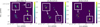 |
Fig. 4 NGC 6153 emission-line maps of [Fe II] 8617 Å, [Fe III] 5270 Å, and [Ni II] 7378 Å. White boxes represent zoomed-in views of smoothed and higher contrast versions of the selected regions. [Ni II] 7378 A emission-line map is scaled down by a factor of 2 from the original. Color-bar values are in units of 10−20 erg s−1 cm−2. |
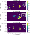 |
Fig. 5 NGC 7009 emission-line maps of [Fe II] 8617 Å, [Fe III] 5270 Å, and [Ni II] 7378 Å. White squares represent zoomed-in views of smoothed and higher contrast versions of the selected regions. [Ni II] 7378 Å emission-line map is scaled down by a factor of 2 from the original. Color-bar values are in units of 10−20 erg s−1 cm−2. |
4.9 NGC 6369
NGC 6369 exhibits a complex structure characterized by a fragmented bright rim around the central star surrounded by some smaller filamentary structures. [Fe II] 7155 Å and 8617 Å, [Ni II] 7378 Å, and [C I] 8727 Å emission lines were detected in this nebula (Figures 9 and A.9). It is worth noting that singly ionized iron and nickel seem to co-exist with atomic carbon and oxygen.
4.10 NGC 6563
Beyond the typical emission lines of PNe, [C I] 8727 Å was also detected in NGC 6563 (Fig. A.10). Most of the emission lines originate from the rim of the nebula.
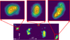 |
Fig. 6 NGC 7009 [O I] 6300 Å emission map with [C I] 8727 Å (black) and [Fe II] 8617 Å (red) contours displayed on top of it. |
4.11 IC 4406
Three new clumps were unveiled at the eastern and western edges of the ellipsoidal PN IC 4406. [Fe II] 7155 Å, 8617 Å, and [Ni II] 7378 Å emission lines emanate directly from the clumps (Fig. 10), while [C I] 8727 Å and [O I] 6300 Å emissions are detected at the central part of the nebula (Fig. A.11). The clumps are also bright in the typical low-ionization lines, such as [N II] and [S II].
4.12 Tc 1
Our analysis of this nebula shows a large knotty and filamentary halo, surrounding the main nebula (Fig. A.12). Emission lines from heavy elements were not detected in the halo, instead they are concentrated in the main spherical shell (Otsuka et al. 2014; Aleman et al. 2019), emanating from small knots. [Fe III] 4881 Å and 5270 Å lines emanate from the very central region of the nebula, while [Fe II] 5158 Å, 7155 Å and 8617 Å, [Ni II] 7378 Å, and [Ca II] 7291 Å originate from the outer knotty shell (Fig. 11). None of these emission lines have been previously reported for this nebula.
5 Discussion
5.1 Correlation of Ni and Fe clumps with PN types
Our analysis of the available MUSE data from a sample of 12 PNe has revealed emission of heavy elements such as Fe and Ni in several clumps. The use of IFU data offers us a unique opportunity to explore the spatial distribution of the [Fe II] 5158 Å, 5262 Å, 7155 Å, and 8617 Å and [Ni II] 7378 Å emission lines for the first time in PNe. [Ni II] and [Fe II] lines were detected in eight out of 12 PNe, and in every case they were found to be co-spatial, verifying the close correlation between these ions (Bautista et al. 1996).
In Table 5, we mention the detection or non-detection of the [Ni II] and [Fe II] lines in different types of PNe. In this table, a summary of our results is also provided, where various PNe types are analyzed. In our study, the term “LIS” refers to discrete, low-ionization regions that are prominent in [N II] and [S II] emission lines, while “Molecule-Rich” PNe denote nebulae where fullerenes, CO, or H2 emissions have been detected. PNe marked with an asterisk (*) are identified as binary candidates based on GAIA measurements (Chornay et al. 2021; Ali & Mindil 2023). Additionally, high-ADF PNe (>5) are likely associated with the presence of a binary system (Wesson et al. 2018). Notably, some studies suggest that LISs are byproducts of common-envelope evolution in binary PNe (Miszalski et al. 2009; Jones & Boffin 2017), a process that can produce soft X-ray emission (Kastner et al. 2012; Freeman et al. 2014).
According to our analysis, Fe- and Ni-rich clumps are found in molecule-rich PNe, X-ray emitting PNe, and, in some cases, PNe with LISs. Moreover, PNe that host a binary system at their center appear to produce such clumps, but more data are needed in order to reach a solid statistical conclusion. Lastly, two PNe of our sample (NGC 6369 and IC 4406), where [Fe II] and [Ni II] lines were detected, host a Wolf-Rayet-type central star.
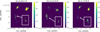 |
Fig. 7 NGC 3132 smoothed emission-line maps of [Fe II] 8617 Å, [Fe III] 5270 Å, and [Ni II] 7378 Å. White boxes represent zoomed-in views of smoothed and higher contrast versions of the new detected regions. Color-bar values are in units of 10−20 erg s−1 cm−2. |
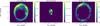 |
Fig. 8 IC 418 emission-line maps of [Fe II] 8617 Å, [Fe III] 5270 Å, and [Ni II] 7378 Å. [Ni II] and [Fe II] emission-line maps are smoothed and scaled down 2 times from the original. Color-bar values are in units of 10−20 erg s−1 cm−2. |
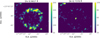 |
Fig. 9 NGC 6369 emission-line maps of [Fe II] 8617 Å and [Ni II] 7378 Å. The emission-line maps are smoothed and scaled down 2 times from the original. Color-bar values are in units of 10−20 erg s−1 cm−2. |
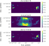 |
Fig. 10 IC 4406 emission-line maps of [Fe II] 8617 Å, [S II] 6716 Å, and [Ni II] 7378 Å. [Fe II] and [Ni II] emission-line maps are smoothed and scaled down 2 times from the original. Color-bar values are in units of 10−20 erg s−1 cm−2. |
5.2 Doubly versus singly ionized iron
The unique capability of IFU data to extract emission-line maps makes it possible to examine the spatial distribution of [Fe III] and [Fe II] emissions. A filamentary structure that extended along the SE-NW direction was unveiled in [Fe III] 5270 Å, probably associated with a hidden jet-like feature in NGC 3242 (Fig. 2). We note that the SE and NW clumps coincide with the k2 and k4 clumps from Gómez-Muñoz et al. (2015) and are likely linked to the interaction between the jet-like structure and the rim. The [Fe III] 5270 Å structure in NGC 6153 is orientated at a higher position angle (150°) than the [Fe II] 8617 Å emitting regions (115°) (Fig. 4). In the case of NGC 3132, the [Fe III] 5270 A line peaks closer to the nebula’s center compared to [Fe II] lines, which is expected given its higher ionization potential. Notably, the SE clump appears brighter and more extended in the doubly ionized iron emission map than in the singly ionized one (Fig. 7). As for NGC 7009, the K2 and K3 clumps (the inner pair of LISs) appear noticeably different in the [Fe III] and [Fe II] lines (Fig. 5). Once again, the former lines show a peak closer to the central star and cover a wider area than the latter. The spatial distribution of [Fe II] in Tc 1 (Fig. 11) matches the knots at the edge of the spherical shell detected in [O I] (Fig. A.12), while [Fe III] emission is concentrated in the inner region around the central star. Lastly, a similar [Fe II] and [Fe III] line distribution is found in IC 418 (Fig. 8).
The observed spatial offset between the singly and doubly ionized iron lines provides clues about their different origins and nature. In addition, emission from singly ionized iron alone is sufficient to compute the total iron abundance in the clumps, as higher-ionization ions are absent (see Sect. 5.8). If both [Fe II] and [Fe III] are excited by shocks, the presence of [Fe III] emission indicates a faster shock, provided that the mechanical energy is sufficient both to release iron from dust and to ionize it twice.
Detection of [Ni II] and [Fe II] in different PN types.
5.3 Ionic, atomic, and molecular stratification of the clump
The expected ionic stratification of clumps illuminated by the UV radiation from the central stars of PNe is illustrated in Fig. 12. High-ionization emission lines, such as [O III], emanate from the H+zone, followed by the [O II] and [S III] lines, which arise near and/or within the H+ → H0 transition zone. MacAlpine et al. (2007) suggested that [C I] emission also arises from this transition zone. Deeper into the clump, [S II] and [N II] lines predominantly originate from the H0 region, while [Ni II], [Fe II], and [O I] arise from the H0 zone and the H0 → H2 transition zone (Hudgins et al. 1990). Finally, CO and possibly PAHs are present in the H2 zone (Boschman et al. 2015).
The low-density fully ionized zone (FIZ) extends from the H0 zone to H+ → H0 transition zone, where strong [S II] and [N II] lines originate (Bautista et al. 1996). [N II] and [O I] are emitted by different regions due to the fact that N+ requires slightly higher energy photons (∼ 14.5 eV) than the O+ (∼ 13.6 eV). Infrared lines of [Ni II] (e.g., 1.191 μm) and [Fe II] (e.g., 1.257 μm and 1.644 μm), which have lower critical densities compared to the optical ones, originate from the H0 zone and lower density gas (FIZs) (Bautista & Pradhan 1998).
In contrast, the high-density, partially ionized zones (∼ 106 cm−3; 10 times denser than FIZs; Bautista & Pradhan 1998) extend from H0 region to H0 → H2 transition zone, where [Ni II], [Fe II], and [O I] lines originate (Bautista et al. 1996). The [Ni II] emission can also extend further into the FIZ than the [Fe II] emission due to its slightly higher ionization potential (18.2 eV vs. 16.2 eV; Lucy 1995). Previous studies on PIZs indicate that the abundance ratio Fe+/O0 is comparable with the Fe/O ratio, suggesting the dominance of Fe+and O0 ions in PIZs (Bautista et al. 1996). This implies that iron depletion in PIZs is likely negligible compared to other ions (Bautista & Pradhan 1998).
The spatial offset between the [Fe II] and [C I] emissions found in NGC 3242 and NGC 7009 LISs supports the aforementioned ionization structure of UV-illuminated clumps (Figs. 3 and 6, respectively). Although the presence of iron in the LISs may suggest a shock interaction, line ratios ([N II]/Hα, [S II]/Hα) from Konstantinou et al. (2025) and Akras et al. (2022) indicate a photo-dominated gas for these cases or only a minor contribution from weak shockwaves. For the remaining PNe in our sample, no spatial offset was measured due to the low spatial resolution of the data or the orientation of the nebulae.
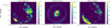 |
Fig. 11 Tc 1 emission-line maps of [Fe II] 8617 Å, [Fe III] 5270 Å, and [Ni II] 7378 Å. [Ni II] and [Fe II] emission-line maps are smoothed. Color-bar values are in units of 10−20 erg s−1 cm−2. |
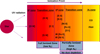 |
Fig. 12 Ionization structure of dense clump illuminated by UV radiation. The zone sizes are not to scale. |
5.4 [Ni II] and [Fe II] emission-line ratios
Given the fact that nickel and iron are co-spatial in gaseous nebulae and possess similar ionization potentials, we explore a possible correlation between these lines’ fluxes. Bautista et al. (1996) explored the correlation between the log (Ni II] 7378 Å/Hα) and log ([Fe II] 8617 Å/Hα) line ratios for a sample of Seyfert galaxies, SNRs, HH objects, and Orion. Their analysis unveiled a one-to-one relationship, including only one photo-dominated source, Orion. Hence, we decided to reconstruct and reexamine the aforementioned ratios, incorporating our PNe findings as well as recent data from the literature (Brugel et al. 1981; Dennefeld & Pequignot 1983; Dennefeld 1986; Russell & Dopita 1990; Osterbrock et al. 1992; Rudy et al. 1994; Rodríguez et al. 2001; Williams et al. 2003; Fang & Liu 2011; García-Rojas et al. 2013; Giannini et al. 2015; Dopita et al. 2018). In total, data from 21 PNe (12 from our study), six HH objects, Orion, and 11 SNRs were used.
The linear correlation between [Ni II] and [Fe II] is demonstrated in Fig. 13. Using a least-squares fitting method, the best-fit line is y=x−0.14, with a goodness of fit for the linear regression of R2 = 0.95. Our best-fit line is slightly different from the 1:1 relation reported by Bautista et al. (1996). Furthermore, the correlation coefficient (i.e., Pearson’s r) for the entire sample is r = 0.97, while for the PNe-Orion subset it is 0.99, and for the SNRs-HH-Seyfert galaxies’ subset it is 0.70. This suggests that the former subset exhibits a higher dispersion than the latter.
Figure 14 illustrates the log ([O I] 6300 Å/Hα) versus log ([Fe II] 8617 Å/Hα) diagram, where a strong correlation between [O I] and [Fe II] is also visible. Once again, we obtained a best fit of y = 0.56 x+0.15, with a goodness of fit for the linear regression of R2 = 0.81. The correlation coefficient of the entire sample is r = 0.90, while for the PNe-Orion and SNRs-HH subsets, it is significantly lower: r = 0.73 and r = 0.61, respectively. These results reflect the higher dispersion of both subsets in the log ([O I] λ 6300/Hα) line ratio. We attribute this increased dispersion to poor sky background subtraction, which is a known issue of MUSE data (Weilbacher et al. 2020).
The error bars in both diagrams represent the fitting procedure error (Sect. 3.1) and should be considered lower limits. Additionally, 2σ confidence ellipses (86.47%) for the emission lines of the two subsets are also shown in both diagrams by red dashed lines (Figs. 13 and 14).
Overall, it is evident that the two subsets — SNRs-Seyfert galaxies-HH objects and PNe-Orion — occupy distinct regions. We argue that these diagrams are very useful for distinguishing shock-dominated and photo-dominated regions.
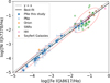 |
Fig. 13 log ([Ni II] 7378 Å/Hα) versus log ([Fe II] 8617 Å/Hα) for SNRs (green), HH (pink), Orion (orange), Seyfert galaxies (brown), PNe (light blue), and PNe from this study (blue). Confidence ellipses (dashed red ellipses) include 86.47% (2σ) of PNe-Orion data points and SNRs-HHSeyfert galaxy data points. |
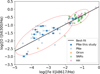 |
Fig. 14 log ([O I] 6300 Å/Hα) versus log ([Fe II] 8617 Å/Hα) for SNRs (green), HH (pink), Orion (orange), PNe (light blue), and PNe from this study (blue). Confidence ellipses (dashed red ellipses) include 86.47% (2 σ) of PNe-Orion data points and SNR-HH data points. |
5.5 Machine-learning clustering and classification
To verify our previous conclusions on the dominated excitation mechanisms in the SNRs-Seyfert galaxies-HH objects and PNe-Orion subsets, the unsupervised machine-learning algorithm K-Means (Hartigan & Wong 1979) was used for clustering our sample. The K-Means algorithm is a type of clustering method that divides data into a predefined number of clusters (in this case two) based on feature similarity. The algorithm works by assigning each data point to the nearest cluster centroid and iteratively updating the centroids until convergence. The resulting shock cluster contains all the HH, Seyfert galaxies, SNRs, and the clumps from IC 4406, while the photoionization cluster includes the Orion, PNe, and the remaining PNe clumps (Fig. 15). To assess the performance of the clustering, we manually split it into three folds, and for each fold we estimated a confusion matrix and all the following metrics. Finally, we present the average confusion matrix (Fig. C.1) and metrics of each fold:
The silhouette score (∼ 0.74) ranges from −1 to 1, where a value closer to 1 indicates well-separated and well-formed clusters.
The Davies-Bouldin index (∼ 0.35) measures the average similarity ratio of each cluster to its most similar one, with lower values indicating better separation.
The Calinsky-Harabasz index (∼ 119) evaluates the ratio of the sum of between-cluster dispersion to within-cluster dispersion, with higher values indicating better clustering.
Excluding IC 4406 values (see Sect. 5.7), we conclude that log ([Ni II] 7378 Å/Hα) and log ([Fe II] 8617 Å/Hα) < −2.20 is the upper limit for photo-dominated regions and the lower limit for shock-dominated regions.
We also examined the theoretical log ([O I] 6300 Å/Hα) versus log ([Fe II] 8617 Å/Hα) diagram by employing the predictions from UV and shock models. Data from the Mexican Million Models database (3 Mdb4, Morisset et al. 2015) were employed. We used photoionization models from project PNe*, which were generated using CLOUDY 17.01 (Ferland et al. 2017). Teff and L for the central source were adopted from Delgado-Inglada & Rodríguez (2014), considering a blackbody energy distribution, the same solar abundances (log (O/H)=−3.36), and a constant density law (see Table D.1).
The grid of shock models (Alarie & Morisset 2019)5 was created using MAPPINGS (Allen et al. 2008; Dopita et al. 2013; Sutherland & Dopita 2017). We selected a grid of complete and incomplete shock models, which are further categorized as fast and slow shocks (for slow shocks, see Alarie & Drissen 2019) with the following properties: (i) solar abundances for fast shocks (Allen et al. 2008) and PNe abundances for the slow shocks (Delgado-Inglada & Rodríguez 2014); (ii) a magnetic-field strength < 10 μG; (iii) pre-shock densities of 10–104 cm−3 for slow shocks and 10–103 cm−3 for fast shocks; (iv) pre-shock temperatures < 15 000 K; (v) cut-off temperatures < 15 000 K (for incomplete shocks only); and (vi) fast- and slow-shock velocities of 100–1000 km/s and 10–100 km/s, respectively (see Table D.2). Similar parameters were employed for PNe analysis in Mari et al. (2023a).
We recall that iron and nickel are primarily locked in dust grains in the interstellar medium. Fast shocks are expected to destroy dust much more efficiently, resulting in highly depleted heavy elements in the gas phase. Since shock models do not account for dust destruction (Allen et al. 2008), the gas-phase abundance of heavy elements, rather than the total (dust + gas) abundance, should be used as input in the shock models. Hence, solar abundances were selected for the fast-shock models, as the subsolar abundances (similar to those observed in PNe) failed to reproduce iron emission for HH objects and SNRs. In HH objects and SNRs environments, where high-velocity shocks are prevalent, significant amounts of iron are released from dust grains into the gas phase (Dopita & Sutherland 1996). Consequently, the solar value (log (Fe/H)=−4.63, Dopita & Sutherland 1996; Allen et al. 2008)6 is more representative than the subsolar PNe abundance (log (Fe/H)=−6.55, Allen et al. 2008; Dopita et al. 2005). Overall, the solar abundance reproduces the observed iron emission in HH objects and SNRs.
The supervised K-nearest neighbors (KNN; Cover & Hart 1967) machine-learning algorithm was also used to train a model with the 3 MdB data and five-fold cross-validation. Then, the model was employed in order to classify the data of our sample. The accuracy of the algorithm is 0.98, while other metrics of the algorithm such as precision, recall, and f1-score are nearly 1 for fast- and slow-shock classes and 0.96, 0.88, and 0.92 for the photoionization class, respectively (confusion matrix in Fig. C.2), indicating that the sample is well separated into three different subgroups (Fig. 16).
All the SNRs and HH objects are located in the fast-shock region. On the other hand, Orion, NGC 3132 SE, NGC 3242 clumps, NGC 6369 SW clump, Tc 1 clumps, He 2-86, M 1-25, IC 418, Pe 1-1, M 1-61, and NGC 7009 (from Fang & Liu 2011) are well placed in the photoionization region. Cn 1-5; M 1-32; M 1-91; the NGC 3132 NW and NE clumps; the NGC 6369 NE clump; and the IC 4406 clumps are located in the fast-shock region, while NGC 6153 clumps and NGC 7009 clumps lie in the slow-shock region. It is worth noting that most of the clumps in NGC 3242, NGC 6153, NGC 7009, and NGC 6369 match the intense [O III]/Hα regions identified by Guerrero et al. (2013), further supporting the shock scenario. We therefore deduce that PNe clumps are more likely excited by shocks (either slow or fast). However, potential contamination of Hα emission by the host nebula may lead to lower line ratios, resulting in their misclassification as photo-dominated regions. Last but not least, in all clumps classified as slow shocks, [C I] 8727 Å is detected.
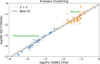 |
Fig. 15 K-means clustering for log ([Ni II] 7378 Å/Hα) versus log ([Fe II] 8617 Å/Hα) diagram. Sources classified as shock-dominated are shown in orange, while photoionized sources are shown in blue. The least-squares best-fit line for all data is represented by a solid black line, and the one-to-one correlation is indicated by a dashed black line. |
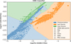 |
Fig. 16 KNN classifier algorithm results for log ([O I] 6300 Å/Hα) versus log ([Fe II] 8617 Å/Hα) diagram. Different colors correspond to different excitation mechanisms, while different markers represent different kinds of objects. |
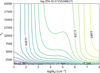 |
Fig. 17 log ([Fe II] 7155 Å/8617 Å) intensity ratio for different Te and ne using B15 atomic data. This diagram is similar for TZ18 atomic data as well. |
5.6 [Fe II] emission lines as an ne diagnostic
The [Fe II] 7155 Å/8617 Å intensity ratio has previously been used to derive electron density in the range of 102–107 cm−3 (Bautista & Pradhan 1998; Bautista et al. 2015). Thus, we reconstructed a grid of [Fe II] line ratios for a wide range of ne and Te values employing PYNEB (Fig. 17). It is evident that the [Fe II] ratio is Te depended on the ne range 103.5–106 cm−3. Therefore, this line ratio should only be used for ne determination below 103.5 cm−3 or above 106 cm−3.
The atomic data from Bautista et al. (2015, hereafter B15) yields densities higher by a factor of 102–104 compared to those derived with the atomic data from Tayal & Zatsarinny (2018, hereafter TZ18, recommended by Mendoza et al. (2023)) for typical observed ratio values (Fig. 18). Due to the complex nature of iron, it is really challenging to model it accurately, and small variations in the atomic data result in significant ne differences (see also Mendoza et al. 2023). The high uncertainties in the [Fe II] 7155 Å/8617 Å åtio for our sample do not allow us to provide robust ne estimates. As a reference, we provide the ne estimated by the mean value of the [Fe II] 7155 Å/8617 Å ratio for the clumps in each PN of our sample: NGC 3242 ∼ 4 · 103 cm−3, NGC 6153 ∼ 3 · 105 cm−3, NGC 7009 ∼ 3 · 103 cm−3, NGC 3132 ∼ 103 cm−3, NGC 6369 ∼ 6 · 105 cm−3, IC 4406 ∼ 5 · 102 cm−3, and Tc 1 ∼ 106 cm−3. Recent JWST observations of the Crab nebula have revealed filamentary structures rich in nickel, with an electron density of ne ∼ 3000 cm−3, assuming Te = 2400 K and infrared [Fe II] diagnostic lines (Temim et al. 2024).
5.7 Nickel-and-iron abundance ratio
In gaseous nebulae where Ni+and Fe+emission lines are prominent, the Ni/Fe abundance ratio is often found to deviate from the solar value. More specifically, super-solar Ni/Fe abundance ratios have been reported in previous studies (e.g., Henry & Fesen 1988; MacAlpine et al. 1989; Hudgins et al. 1990; Jerkstrand et al. 2015a; Temim et al. 2024). Super-solar Ni/Fe abundance ratios have also been estimated by Bautista et al. (1996), Dennefeld (1986), Maguire et al. (2018), and Liu et al. (2023) under the assumption that Ni/Fe = Ni+/Fe+, since singly ionized atoms are expected to dominate partially ionized regions. Higher ionization state ions were either absent (e.g., Ni+2) or originated from different structures (e.g., Fe+2).
Nonetheless, one must be careful when relying on the Ni/Fe = Ni+/Fe+assumption for determining the gas-phase abundance ratios. In particular, one must consider the exposure of clumps to the hard UV radiation from hot central stars and/or shocks, both of which can result in non-negligible fractions of doubly ionized iron and nickel. For this reason, before employing the aforementioned assumption, we: 1) compared the spatial distribution of singly and doubly ionized iron emission lines (see Sect. 5.2); 2) thoroughly tested the validity of this assumption in a case study (see Sect. 5.8); and 3) searched for a potential detection of doubly ionized nickel emission lines in MUSE wavelength coverage.
For our sample of PNe clumps, the Ni/Fe abundance ratios were derived from the optical lines and the PYNEB package, considering iron atomic data from B15 and TZ18, and nickel atomic data from Chianty v10.1 (Del Zanna et al. 2021). Assuming Te = 10 000 K and ne = 1000 cm−3 (Akras et al. 2022; Mari et al. 2023a, b), the overall Ni/Fe ratio is found to be close to the solar value (0.058, Lodders et al. 2009) (orange and blue dots in Fig. 19).
If fluorescence excitation of the [Ni II] 7378 Å line is taken into account, the resulting abundances from our sample are significantly lower than the solar value (purple dot in Fig. 20). Similarly, Fig. 19 shows that only in the no-fluorescence case (orange and blue dots), the Ni/Fe abundance ratio reaches its solar value, indicating that fluorescence excitation should be negligible, as expected in low-excitation regions (Zhang & Liu 2006). For the former calculation, we adopted ∼ 80% fluorescent contribution in [Ni II] 7378 Å emission, based on models for the Orion nebula by Lucy (1995).
Delgado-Inglada et al. (2016) (hereafter DI16) investigated the Ni/Fe abundance ratio in PNe using the [Fe III] and [Ni III] optical lines. These authors argued that nickel atoms are more efficiently trapped in dust grains compared to iron atoms, which would explain their subsolar value. However, more recent studies have challenged this interpretation. Temim et al. (2024) suggested that emission lines from doubly ionized nickel and iron underestimate the Ni/Fe abundance ratio, because Ni+2 originates from lower temperature and lower density regions compared to Fe+2. Additionally, Méndez-Delgado et al. (2021) derived unexpected Ni+2 abundance estimates based on [Ni III] emission lines and attributed them to inaccuracies in the available atomic data, which could further explain the subsolar Ni/Fe value reported by DI16.
To ensure that the Ni/Fe abundance ratios of the clumps in our sample of PNe are reliable, we examined the extreme supersolar Ni/Fe abundance ratio – 60–75 times above the solar value – of the Crab nebula reported by MacAlpine et al. (1989, 2007). For this exercise, we used PYNEB along with the iron atomic data from B15/TZ18 and the nickel atomic data from Chianti v10.1. Assuming Ni/Fe = Ni+/Fe+, we found an Ni/Fe abundance ratio only 5.5-7 times above the solar value from Lodders et al. (0.058, 2009) and 6–7.5 times from Scott et al. (0.053, 2015). Our values for the Crab nebula are consistent with those recently derived by Temim et al. (2024).
All PNe in our sample, except for IC 4406, have Ni and Fe chemical abundances well below the solar value (Fig. 20). This suggests that Fe and Ni are either highly ionized (e.g., Ni+2 and Fe+2) in the clumps, and the assumption Ni/Fe = Ni+/Fe+ leads to an underestimation of the abundances, or that both elements are depleted in dust grains. The latter scenario is the most probable, as PNe are not expected to have shocks capable of destroying large amounts of dust. Even in more extreme environments, such as HH objects, only ∼ 30–67% of dust is destroyed (Mesa-Delgado et al. 2009; Méndez-Delgado et al. 2022). Additionally, [Ni III] and [Fe III] are not detected in the clumps of our PNe sample.
As for IC 4406, iron and nickel abundances are significantly higher than the corresponding solar values. The faint emission lines measured in the nebula result in highly uncertain flux measurements, despite their indisputable detection. Therefore, we decided not to include IC 4406 in the following iron and nickel depletion calculations.
The correlation between the Ni and Fe depletion factors7 is illustrated in Fig. 21 (with and without fluorescence). The slopes of the best-fit lines for our sample (0.83), obtained using the least-squares method (R2 = 0.98 and Pearson’s r = 0.99), are in excellent agreement with previous studies (DI16: y = 0.85 x− 0.03), using the same solar abundance data (Lodders et al. 2009). However, our vertical intercept differs from the previous studies by −0.42 (B15) and −0.49 (TZ18) or by +0.17 (B15) and +0.1 (TZ18), depending on whether fluorescence excitation is taken into account or not, respectively. This discrepancy is probably caused by the different nickel and iron ions used in the two studies (singly ionized in our study, doubly ionized in DI16).
Overall, our sample exhibits a correlation between nickel and iron depletion factors, which vary over a wide range (spanning approximately 2.5 dex for Ni and 2 dex for Fe), which supports the validity of our abundances. We also concluded that a significant amount of Fe (and Ni) still remains locked in dust grains.
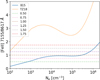 |
Fig. 18 ne calculated from [Fe II] 7155 Å/8617 Å intensity ratio for Te = 10000 K using atomic data from B15 (blue lines) and TZ18 (orange line). Typical observed values of the ratio are shown by dashed colored lines. |
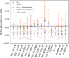 |
Fig. 19 Ni/Fe abundance ratio for each clump in our sample of PNe. All the abundances have been calculated for Te = 10 000 K and ne = 1000 cm−3 and Chianty v10.1 atomic data for nickel. The dashed black horizontal line corresponds to the iron solar abundance from Lodders et al. (2009). Green and blue dots were estimated utilizing B15 atomic data, and the former account for fluorescence in nickel emission. Similarly, the pink and orange dots represent TZ18 atomic data. |
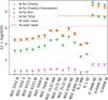 |
Fig. 20 Ni and Fe abundances, assuming Ni/H = Ni+/H+and Fe/H = Fe+/H+, respectively. All the abundances were calculated for Te = 10 000 K and ne = 1000 cm−3 and Chianty v10.1 atomic data for nickel. The dashed pink and brown horizontal lines correspond to the solar abundance of nickel and iron, respectively. Green and purple dots correspond to nickel abundance, with the last ones accounting for fluorescence. Blue and orange dots corresponds to iron abundance utilizing B15 and TZ18 atomic data, respectively. |
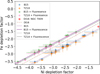 |
Fig. 21 Ni depletion factor versus Fe depletion factor in clump regions within PNe. Diamond shapes correspond to NGC 7009 values. All the clump abundances were calculated for Te = 10 000 K and ne = 1000 cm−3. Solid lines correspond to best-fit lines for different iron atomic data and fluorescent cases for nickel. The dashed line shows the best fit from DI16. Green and blue dots were estimated accounting for fluorescence (or lack thereof) in nickel using B15 atomic data. The pink and orange dots were derived with the TZ18 atomic data. |
5.8 The case study of NGC 7009
NGC 7009 is an ideal source to examine Fe depletion using various techniques: (i) analyzing singly ionized lines under the assumption that Fe/H = Fe+/H+, (ii) combining singly and doubly ionized lines, and (iii) applying an ionization correction factor (ICF) to the doubly ionized lines.
The outer pair of LISs (K1 and K4, Gonçalves et al. 2003) was only detected in the singly ionized lines, whereas both singly and doubly ionized lines are present in the inner pair (K2 and K3). The depletion factors for the outer LISs are −2.4 (K1) and −2.6 (K4), with a relative error of ± 0.3. For the inner LISs, we compute depletion factors of −2.3 (K2) and −2.6 (K3), assuming Fe = Fe++Fe+2, Te = 10 000 K, and ne = 5000 cm−3 (Akras et al. 2022). The agreement between the depletion factors of the inner and outer LISs supports our hypothesis that the latter are Fe+ dominated, validating our assumption that Fe/H = Fe+/H+. If we only consider the [Fe III] lines for the inner LISs and apply the ICF (Fe+2) formulae from Rodríguez & Rubin (2005), the iron depletion factors are overestimated, ranging from −1.75 to −2.3.
It should be noted that our Fe depletion values are significantly lower than the value of −1.18 (red diamond in Fig. 21) reported by DI16, which was derived using the [Fe III] lines detected by Fang & Liu (2011). To verify the reliability of our estimates, we recalculated the depletion using the same data (Fang & Liu 2011) and the ICF formulae 2 and 3 from Rodríguez & Rubin (2005). The first ICF, based on photoionization models, yields a depletion factor of −1.18, consistent with the value reported by DI16. However, the second ICF, based on observational data, produces a value of −2.02, which is closer to our estimates.
We also computed the Fe depletion from the MUSE data by simulating the slit spectrum (position and orientation) from Fang & Liu (2011) using the SATELLITE code (Akras et al. 2022). This analysis yielded Fe depletion factors of −2.11 and −2.57, based on the [Fe III] 4881 Å line and the ICF formulae from Rodríguez & Rubin (2005), respectively. These values are consistent with our findings for both pairs of LISs. It should be noted that the observational ICF generally results in lower depletion factors compared to the theoretical ICF.
Regarding nickel, we computed a depletion factor of −2.3 for the outer LISs. We argue that our value is reliable due to the strong one-to-one relationship between the Fe and Ni depletion factors (Fig. 21). For the inner LISs, we estimated depletion factors of −3.1 and −3.4 for K2 and K3, respectively, considering only the [Ni II] 7378 Å line ([Ni III] is not detected). Based on our previous analysis, we expect comparable Ni depletion factors for the inner and outer LISs, as observed for Fe. Our Ni depletion factors are again lower than the value of −1.11 reported by DI16. Overall, the outer pair of LISs in NGC 7009 exhibits a high Ni+/Ni+2 ratio, making the assumption of Ni/H ∼ Ni+/H+, which is adequate for abundance estimations.
Lastly, according to the KNN algorithms (Figs. 15 and 16), the inner LISs (K2 and K3) are classified as photo-dominated, whereas the outer LISs (K1 and K4) are classified as slow-shock-dominated (Table 6). This distinction is expected, as K2 and K3, being closer to the central star, are exposed to more intense UV radiation. Therefore, the physical processes taking place in the two pairs of LISs in NGC 7009 are considerably different.
Emission-line ratios including [O I] 6300 Å, [Fe II] 8617 Å, and [Ni II] 7378 Å for the two pairs of LISs in NGC 7009.
6 Conclusions
6.1 Origin of Ni and Fe emissions in gaseous nebulae
Heavy elements such as nickel and iron originate either from type Ia supernovae (thermonuclear explosion of accreting white dwarfs; e.g., RCW 86 and Kepler’s nebula; Dennefeld 1986) or from core-collapse supernovae, where they are produced in the silicon-burning shell of massive stars (Jerkstrand et al. 2015b, a). After being ejected into the interstellar medium and potentially interacting with stellar winds, they are finally condensed into dust grains (e.g., Barlow 1978) in H II regions and molecular interstellar clouds (e.g., Mesa-Delgado et al. 2009).
The detection of Ni+and Fe+in gaseous nebulae can be explained by the fact that fast shocks (most commonly found in SNRs and HH objects) can efficiently destroy dust grains through thermal and nonthermal sputtering in the gas behind the shock front, as well as through grain-grain collisions (Hollenbach et al. 1989; Jones et al. 1994; Mouri & Taniguchi 2000). Through these mechanisms, the elements are released back into the gas phase, making it possible to estimate their gas-phase abundances. Despite the fact that fast shocks effectively destroy dust, in slower shocks, dust destruction is incomplete until the recombination zone of the shock has been reached (Dopita et al. 2018). For instance, Mesa-Delgado et al. (2009) estimated in HH 202 (an HH object in the Orion nebula) that iron and nickel abundances increase by up to a factor of ten after the passage of a shockwave that destroys 30% to 50% of the dust, while Méndez-Delgado et al. (2022) studied HH514 and found ∼ 67% dust destruction.
Our analysis of 16 clumps in seven host PNe has shown that the clumps in NGC 3132 NW and NE, NGC 6369 NE, and IC 4406, where the highest Ni and Fe abundances are found, are also classified as fast-shock-dominated (Fig. 16). These results corroborate that fast shocks are more efficient in destroying dust than slow shocks (Fig. 20). In the case of IC 4406, the clumps exhibit a high log ([S II]/Hα) ratio, ranging from −0.30 to −0.05, which further supports the shock hypothesis (Sabbadin et al. 1977; Leonidaki et al. 2013; Kopsacheili et al. 2020; Akras et al. 2020b). It is worth noting that ten out of 16 clumps in our sample of PNe, where Ni+and Fe+were detected, are located within confirmed or candidate binary systems (Table 5). This suggests that clump formation may be somehow associated with binary interactions.
6.2 Clump-formation scenarios
Two main mechanisms for clump formation have been proposed, as described by Matsuura et al. (2009). Clumps may form either during the AGB phase due to localized density enhancements or those in situ at the beginning of the PN phase.
Clumps can form by inhomogeneities in the stellar wind of the progenitor star (Bertoldi 1989; Reipurth 1983; Soker 1998). If these stellar winds were intrinsically knotty, probably due to binary interactions (Edgar et al. 2008), the ejected clumps could evolve by merging with material previously or subsequently expelled from the central region (Meaburn et al. 2000). Therefore, the outer clumps are older than the inner ones. In this scenario, the narrow [Ni II] and [Fe II] emission lines are expected to originate from the dense, mainly neutral knots, which are being swept up by the fast stellar wind. The broader [N II] and [S II] lines are associated from a bow shock surrounding the clumps, created by the clump-wind velocity difference. For example, a velocity difference of ∼ 30 km/s between [N II] and [Ni II] emissions has been observed in P-Cygni (Barlow et al. 1994).
As a result, the broad [N II] and [S II] lines should appear less clumpy than the narrow [Ni II] and [Fe II] lines, since they arise from a larger volume (Meaburn et al. 2000). Thus, observable velocity differences among various species in such clumps could help pinpoint their emission regions, whether within the molecular core or the bow shock. Furthermore, detecting distinct velocity components within clumps would support the hypothesis that clumps form through stellar-wind inhomogeneities, which in turn could indicate the presence of a binary system in the nebula. To test this hypothesis, high-spectral-resolution observations of clumps embedded in PNe are necessary to gain insights into their formation history.
Another possible scenario for clump formation suggests that Ni+and Fe+are formed in situ, in small, dense regions that are illuminated by high-energy photons. The intense UV radiation from the central star ionizes the nebula, and the ionization front propagates through the gas. However, the ionization front is not smooth or in pressure equilibrium with the ambient gas, as hydrodynamical models have shown (Bedijn & Tenorio-Tagle 1981), and this could lead to the formation of turbulent instabilities (Reyleigh-Taylor). Turbulent instabilities could also form from the interaction between the slow and fast progenitor winds (García-Segura et al. 2006). In this scenario, clumps situated closer to the central star are expected to be older than those located further away.
The H atoms are ionized on the side of the gas facing the central star and emit photoelectrons toward the molecular gas (photoevaporation flow). At the same time, the temperature in this region increases along with the pressure, which forces the gas to expand. Therefore, the hot ionized gas compresses the rest of the molecular gas on the outer side, while it expands freely toward the central star. Due to conservation of momentum, the remaining cold molecular gas starts moving outwards, as in a rocket-jet system. Thus, this “rocket effect” (Oort & Spitzer 1955; Mellema et al. 1998) can create highly condensed and compressed clump regions.
7 Summary
This study focused on the presence of low-ionization Ni and Fe emission lines in planetary nebulae. Using MUSE IFU archival data, we detected nickel and iron emission lines in seven PNe. Specifically, we identified 16 clump structures rich in nickel and iron. The most prominent lines of these heavy elements were [Ni II] 7378 Å and [Fe II] 8617 Å.
New clumps were discovered in NGC 3132 and IC 4406. [Ni II] and [Fe II] emission lines were found to emanate directly from the LISs in NGC 3242, NGC 6153, and NGC 7009. A spatial offset of 0.5–1′′ between the [Fe II] 8617 Å and [C I] 8727 Å was measured for the LISs of NGC 3242 and NGC 7009. The peak of the [Fe II] 8617 Å line was found to be further away from the central star in the NGC 3242 clumps and the K4 clump in NGC 7009.
From our analysis, these small, discrete, and isolated structures show a possible link with binarity, X-ray emission, and molecule-rich PNe. In some cases, they appear to be co-spatial with the LIS already detected in characteristic emission lines (e.g., [N II]). However, we kept our sample small in order to provide significant statistical results.
The hypothesis that nickel and iron co-exist in such clumps in a wide variety of gaseous nebulae was tested through the log ([Ni II] 7378 Å/Hα) versus log ([Fe II] 8617 Å/Hα) diagram, and a strong correlation was found. log ([Ni II] 7378 Å/Hα) and log ([Fe II] 8617 Å/Hα) < −2.20 very likely define the boundary zone between shock-dominated (HH objects and SNRs) and photo-dominated nebulae (PNe and Orion).
From the log ([O I] 6300 Å/Hα) versus log ([Fe II] 8617 Å/Hα) diagram and a machine-learning-algorithm approach, distinct regimes were found to distinguish shock-dominated and photo-dominated gases. Ten out of 16 clumps in our sample were classified as shock-excited. Highvelocity shocks exhibit extensive dust destruction and are characterized by higher depletion factors.
Moreover, the electron density was examined using the [Fe II] 7155 Å/8617 Å diagnostic-line ratio. This ratio only seems to be sensitive to density below 103.5 cm−3 or above 106 cm−3. In addition, different atomic data resulted in significant variations in the results.
The Ni/Fe abundance ratio derived for the clumps in our PNe sample was calculated using different atomic data, assuming Ni/Fe ∼ Ni+/Fe+and considering the possible contribution of fluorescence in the [Ni II] 7378 Å. Our Ni/Fe values are systematically below or close to the solar value. This result supports the idea that nickel atoms are stuck more efficiently on dust grains than iron atoms. The fact that both Ni and Fe abundances are below their solar value suggests that either higher ionization state ions are present or that a significant fraction of nickel and iron atoms remain depleted in dust grains. Given that shocks can partially destroy dust grains depending on their velocity, the depletion scenario seems more probable. Furthermore, the absence of detectable [Fe III] and [Ni III] emission in PNe clumps – at least within the MUSE optical wavelength range – further supports the depletion scenario.
In the particular case of NGC 7009, both the inner (K2, K3) and the outer (K1, K4) pairs of LISs exhibit comparable iron and nickel depletion, as expected. The detection of doubly ionized iron in the inner LISs, while being absent in the outer LISs is likely a key factor to improving our understanding of the formation, evolution, and origin of LISs in PNe.
Acknowledgements
We are grateful to the anonymous referee for their constructive comments, which helped improve the content and the clarity of this work. We also thank Jeremy Walsh for kindly providing the reduced data cube of Tc 1. We wish to thank the “Summer School for Astrostatistics in Crete” for providing training on the statistical methods adopted in this work. The research project is implemented in the framework of H.F.R.I call “Basic research financing (Horizontal support of all Sciences)” under the National Recovery and Resilience Plan “Greece 2.0” funded by the European Union – NextGenerationEU (H.F.R.I. Project Number: 15665). JGR acknowledges financial support from the Agencia Estatal de Investigación of the Ministerio de Ciencia e Innovación (AEI- MCINN) under Severo Ochoa Centres of Excellence Programme 2020-2023 (CEX2019-000920-S), and from grant PID-2022136653NA-I00 (DOI:10.13039/501100011033) funded by the Ministerio de Ciencia, Innovación y Universidades (MCIU/AEI) and by ERDF “A way of making Europe” of the European Union. DRG acknowledges FAPERJ (E-26/200.527/2023) and CNPq (403011/2022-1; 315307/2023-4) grants. The results from NGC 7009, NGC 3132, IC 418, NGC 6369, NGC 6563 and IC 4406 are based on public data released from the MUSE commissioning observations at the VLT Yepun (UT4) telescope under Programs ID 60.A-9347(A), 60.A9100(A), 60.A-9100(H) and 60.A-9100(G), respectively. Lastly, NGC 6369 and IC 4406 analysis is based on data obtained from the ESO Science Archive Facility with DOI: https://doi.org/10.18727/archive/41.
Appendix A Supplementary emission-line maps
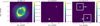 |
Fig. A.1 NGC 3242 emission-line maps of Hβ, [O I] 6300 Å and [C I] 8727 Å. The regions where fluxes were measured are displayed on the [O I] 6300 Å map. Color-bar values are in units of 10−20 erg s−1 cm−2. |
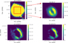 |
Fig. A.5 M 1-42 emission-line maps of [N II], Hβ, [O I] 6300 Å and [C I] 8727 Å. Numbers 1 to 5 denote the different LISs aligned along the major axis of the PN. |
Appendix B Integrated spectrum
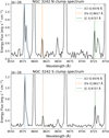 |
Fig. B.1 The spectrum of two nebular structures (N and S clumps) in NGC 3242. The [Cl II] 8578 Å, [Fe II] 8617 Å and [C I] 8727 Å emissions lines are indicated with blue, orange and green vertical dot lines, respectively. H I 8598 Å and 8665 Å, He I 8649 Å and 8733 Å emissions are also present in the plot. The number in the top left corner indicates the scaling factor applied in the y-axis values. |
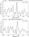 |
Fig. B.2 The spectrum of two nebular structures (N and S clumps) in NGC 3242 covering the wavelength range from 7350 to 7400 Å. The [Ni II] 7378 A emission line is indicated with blue vertical dot line. The number in the top left corner indicates the scaling factor applied in the y-axis values. |
Appendix C Extra Figures
 |
Fig. C.1 Mean confusion matrix for K-Means classifier. |
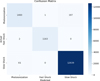 |
Fig. C.2 Confusion matrix for KNN classifier. |
Appendix D Extra Tables
Parameters selected for the photoinization models from 3Mdb database.
Parameters selected for the shock models from 3Mdb database.
References
- Akras, S., & Gonçalves, D. R., 2016, MNRAS, 455, 930 [NASA ADS] [CrossRef] [Google Scholar]
- Akras, S., Gonçalves, D. R., Ramos-Larios, G., & Aleman, I., 2020a, MNRAS, 493, 3800 [Google Scholar]
- Akras, S., Monteiro, H., Aleman, I., et al. 2020b, MNRAS, 493, 2238 [Google Scholar]
- Akras, S., Monteiro, H., Walsh, J. R., et al. 2022, MNRAS, 512, 2202 [NASA ADS] [CrossRef] [Google Scholar]
- Akras, Aleman, I., Gonçalves, D. R., Ramos-Larios, G., & Bouvis, K. 2024a, A&A, 689, A70 [NASA ADS] [CrossRef] [EDP Sciences] [Google Scholar]
- Akras, Monteiro, H., Walsh, J. R.,, et al. 2024b, A&A, 689, A14 [NASA ADS] [CrossRef] [EDP Sciences] [Google Scholar]
- Alarie, A., & Drissen, L., 2019, MNRAS, 489, 3042 [NASA ADS] [CrossRef] [Google Scholar]
- Alarie, A., & Morisset, C., 2019, Rev. Mexicana Astron. Astrofis., 55, 377 [Google Scholar]
- Aleman, I., Leal-Ferreira, M. L., Cami, J., et al. 2019, MNRAS, 490, 2475 [NASA ADS] [CrossRef] [Google Scholar]
- Ali, A., & Dopita, M. A., 2017, PASA, 34, e036 [NASA ADS] [CrossRef] [Google Scholar]
- Ali, A., & Mindil, A., 2023, Res. Astron. Astrophys., 23, 045006 [Google Scholar]
- Ali, A., Amer, M. A., Dopita, M. A., Vogt, F. P. A., & Basurah, H. M., 2015, A&A, 583, A83 [NASA ADS] [CrossRef] [EDP Sciences] [Google Scholar]
- Allen, M. G., Groves, B. A., Dopita, M. A., Sutherland, R. S., & Kewley, L. J., 2008, ApJS, 178, 20 [Google Scholar]
- Argyriou, I., Glasse, A., Law, D. R., et al. 2023, A&A, 675, A111 [NASA ADS] [CrossRef] [EDP Sciences] [Google Scholar]
- Bacon, R., Accardo, M., Adjali, L., et al. 2010, SPIE Conf. Ser., 7735, 773508 [Google Scholar]
- Balick, B., 1987, AJ, 94, 671 [NASA ADS] [CrossRef] [Google Scholar]
- Barlow, M. J., 1978, MNRAS, 183, 367 [NASA ADS] [CrossRef] [Google Scholar]
- Barlow, M. J., Drew, J. E., Meaburn, J., & Massey, R. M., 1994, MNRAS, 268, L29 [Google Scholar]
- Bautista, M. A., & Pradhan, A. K., 1998, ApJ, 492, 650 [NASA ADS] [CrossRef] [Google Scholar]
- Bautista, M. A., Peng, J., & Pradhan, A. K., 1996, ApJ, 460, 372 [Google Scholar]
- Bautista, M. A., Fivet, V., Ballance, C., et al. 2015, ApJ, 808, 174 [NASA ADS] [CrossRef] [Google Scholar]
- Bedijn, P. J., & Tenorio-Tagle, G., 1981, A&A, 98, 85 [NASA ADS] [Google Scholar]
- Bertoldi, F., 1989, ApJ, 346, 735 [Google Scholar]
- Böker, T., Arribas, S., Lützgendorf, N., et al. 2022, A&A, 661, A82 [NASA ADS] [CrossRef] [EDP Sciences] [Google Scholar]
- Bond, H. E., 2000, in Astronomical Society of the Pacific Conference Series, 199, Asymmetrical Planetary Nebulae II: From Origins to Microstructures, eds. J. H. Kastner, N. Soker, & S. Rappaport, 115 [Google Scholar]
- Boschman, L., Cazaux, S., Spaans, M., Hoekstra, R., & Schlathölter, T., 2015, A&A, 579, A72 [NASA ADS] [CrossRef] [EDP Sciences] [Google Scholar]
- Bouvis, K., Akras, S., Monteiro, H., et al. 2025, MNRAS, staf 1042 [Google Scholar]
- Brugel, E. W., Boehm, K. H., & Mannery, E., 1981, ApJS, 47, 117 [Google Scholar]
- Cala, R. A., Miranda, L. F., Gómez, J. F., et al. 2024, A&A, 691, A321 [NASA ADS] [CrossRef] [EDP Sciences] [Google Scholar]
- Cami, J., Bernard-Salas, J., Peeters, E., & Malek, S. E., 2010, Science, 329, 1180 [NASA ADS] [CrossRef] [Google Scholar]
- Chornay, N., Walton, N. A., Jones, D., et al. 2021, A&A, 648, A95 [NASA ADS] [CrossRef] [EDP Sciences] [Google Scholar]
- Corradi, R. L. M., Perinotto, M., Schwarz, H. E., & Claeskens, J. F., 1997, A&A, 322, 975 [Google Scholar]
- Courtes, G., Georgelin, Y., Monnet, R. B. G., & Boulesteix, J., 1988, in Instrumentation for Ground-Based Optical Astronomy, 266 [Google Scholar]
- Cover, T., & Hart, P., 1967, IEEE Trans. Inform. Theory, 13, 21 [CrossRef] [Google Scholar]
- De Marco, O., Akashi, M., Akras, S., et al. 2022, Nat. Astron., 6, 1421 [Google Scholar]
- Del Zanna, G., Dere, K. P., Young, P. R., & Landi, E., 2021, ApJ, 909, 38 [NASA ADS] [CrossRef] [Google Scholar]
- Delgado-Inglada, G., & Rodríguez, M., 2014, ApJ, 784, 173 [NASA ADS] [CrossRef] [Google Scholar]
- Delgado-Inglada, G., Mesa-Delgado, A., García-Rojas, J., Rodríguez, M., & Esteban, C., 2016, MNRAS, 456, 3855 [NASA ADS] [CrossRef] [Google Scholar]
- Dennefeld, M., 1986, A&A, 157, 267 [NASA ADS] [Google Scholar]
- Dennefeld, M., & Pequignot, D., 1983, A&A, 127, 42 [Google Scholar]
- Díaz-Luis, J. J., García-Hernández, D. A., Manchado, A., et al. 2018, AJ, 155, 105 [Google Scholar]
- Dopita, M. A., & Sutherland, R. S., 1996, ApJS, 102, 161 [Google Scholar]
- Dopita, M. A., Groves, B. A., Fischera, J., et al. 2005, ApJ, 619, 755 [Google Scholar]
- Dopita, M. A., Sutherland, R. S., Nicholls, D. C., Kewley, L. J., & Vogt, F. P. A., 2013, ApJS, 208, 10 [NASA ADS] [CrossRef] [Google Scholar]
- Dopita, M. A., Ali, A., Sutherland, R. S., Nicholls, D. C., & Amer, M. A., 2017, MNRAS, 470, 839 [NASA ADS] [CrossRef] [Google Scholar]
- Dopita, M. A., Vogt, F. P. A., Sutherland, R. S., et al. 2018, ApJS, 237, 10 [NASA ADS] [CrossRef] [Google Scholar]
- Edgar, R. G., Nordhaus, J., Blackman, E. G., & Frank, A., 2008, ApJ, 675, L101 [Google Scholar]
- Eisenhauer, F., Abuter, R., Bickert, K., et al. 2003, SPIE Conf. Ser., 4841, 1548 [Google Scholar]
- Fang, X., & Liu, X. W., 2011, MNRAS, 415, 181 [NASA ADS] [CrossRef] [Google Scholar]
- Ferland, G. J., Chatzikos, M., Guzmán, F., et al. 2017, Rev. Mexicana Astron. Astrofis., 53, 385 [Google Scholar]
- Freeman, M., Montez, R. J., Kastner, J. H., et al. 2014, ApJ, 794, 99 [NASA ADS] [CrossRef] [Google Scholar]
- Frew, D. J., 2008, PhD thesis, Macquarie University, Department of Physics and Astronomy, Australia [Google Scholar]
- Frew, D. J., Bojičić, I. S., & Parker, Q. A., 2013, MNRAS, 431, 2 [NASA ADS] [CrossRef] [Google Scholar]
- García-Segura, G., López, J. A., Steffen, W., Meaburn, J., & Manchado, A., 2006, ApJ, 646, L61 [CrossRef] [Google Scholar]
- García-Rojas, J., Peña, M., Morisset, C., et al. 2013, A&A, 558, A122 [NASA ADS] [CrossRef] [EDP Sciences] [Google Scholar]
- García-Rojas, J., Madonna, S., Luridiana, V., et al. 2015, MNRAS, 452, 2606 [CrossRef] [Google Scholar]
- García-Rojas, J., Delgado-Inglada, G., García-Hernández, D. A., et al. 2018, MNRAS, 473, 4476 [CrossRef] [Google Scholar]
- García-Rojas, J., Morisset, C., Jones, D., et al. 2022, MNRAS, 510, 5444 [CrossRef] [Google Scholar]
- Giannini, T., Antoniucci, S., Nisini, B., Bacciotti, F., & Podio, L., 2015, ApJ, 814, 52 [NASA ADS] [CrossRef] [Google Scholar]
- Gil de Paz, A., Carrasco, E., Gallego, J., et al. 2018, SPIE Conf. Ser., 10702, 1070217 [NASA ADS] [Google Scholar]
- Gómez-Llanos, V., García-Rojas, J., Morisset, C., et al. 2024, A&A, 689, A228 [NASA ADS] [CrossRef] [EDP Sciences] [Google Scholar]
- Gómez-Muñoz, M. A., Blanco Cárdenas, M. W., Vázquez, R., et al. 2015, MNRAS, 453, 4175 [NASA ADS] [Google Scholar]
- Gonçalves, D. R., Corradi, R. L. M., & Mampaso, A., 2001, ApJ, 547, 302 [CrossRef] [Google Scholar]
- Gonçalves, D. R., Corradi, R. L. M., Mampaso, A., & Perinotto, M., 2003, ApJ, 597, 975 [CrossRef] [Google Scholar]
- González-Santamaría, I., Manteiga, M., Manchado, A., et al. 2021, A&A, 656, A51 [NASA ADS] [CrossRef] [EDP Sciences] [Google Scholar]
- Graham, J. R., Wright, G. S., & Longmore, A. J., 1987, ApJ, 313, 847 [NASA ADS] [CrossRef] [Google Scholar]
- Guerrero, M. A., Toalá, J. A., Medina, J. J., et al. 2013, A&A, 557, A121 [NASA ADS] [CrossRef] [EDP Sciences] [Google Scholar]
- Halpern, J. P., & Oke, J. B., 1986, ApJ, 301, 753 [Google Scholar]
- Hartigan, J. A., & Wong, M. A., 1979, J. Roy. Statist. Soc. Ser. C (Appl. Statist.), 28, 100 [Google Scholar]
- Henry, R. B. C., & Fesen, R. A., 1988, ApJ, 329, 693 [Google Scholar]
- Hollenbach, D. J., Chernoff, D. F., & McKee, C. F., 1989, in Infrared Spectroscopy in Astronomy, ed. E. Böhm-Vitense, 245 [Google Scholar]
- Hudgins, D., Herter, T., & Joyce, R. J., 1990, ApJ, 354, L57 [Google Scholar]
- Hyung, S., 1994, ApJS, 90, 119 [Google Scholar]
- Icke, V., 1988, A&A, 202, 177 [NASA ADS] [Google Scholar]
- Jerkstrand, A., Smartt, S. J., Sollerman, J., et al. 2015a, MNRAS, 448, 2482 [Google Scholar]
- Jerkstrand, A., Timmes, F. X., Magkotsios, G., et al. 2015b, ApJ, 807, 110 [Google Scholar]
- Jones, D., & Boffin, H. M. J., 2017, Nat. Astron., 1, 0117 [Google Scholar]
- Jones, A. P., Tielens, A. G. G. M., Hollenbach, D. J., & McKee, C. F., 1994, ApJ, 433, 797 [NASA ADS] [CrossRef] [Google Scholar]
- Jones, D., Wesson, R., García-Rojas, J., Corradi, R. L. M., & Boffin, H. M. J., 2016, MNRAS, 455, 3263 [NASA ADS] [CrossRef] [Google Scholar]
- Kastner, J. H., Montez, R. J., Balick, B.,, et al. 2012, AJ, 144, 58 [NASA ADS] [CrossRef] [Google Scholar]
- Kastner, J. H., Wilner, D. J., Moraga Baez, P., et al. 2024, ApJ, 965, 21 [Google Scholar]
- Konstantinou, L., Akras, S., Garcia-Rojas, J., et al. 2025, A&A, 697, A227 [NASA ADS] [CrossRef] [EDP Sciences] [Google Scholar]
- Kopsacheili, M., Zezas, A., & Leonidaki, I., 2020, MNRAS, 491, 889 [CrossRef] [Google Scholar]
- Kwok, S., Purton, C. R., & Fitzgerald, P. M., 1978, ApJ, 219, L125 [CrossRef] [Google Scholar]
- Le Fèvre, O., Saisse, M., Mancini, D., et al. 2003, SPIE Conf. Ser., 4841, 1670 [Google Scholar]
- Leonidaki, I., Boumis, P., & Zezas, A., 2013, MNRAS, 429, 189 [NASA ADS] [CrossRef] [Google Scholar]
- Liu, X. W., Storey, P. J., Barlow, M. J., et al. 2000, MNRAS, 312, 585 [NASA ADS] [CrossRef] [Google Scholar]
- Liu, X. W., Luo, S. G., Barlow, M. J., Danziger, I. J., & Storey, P. J., 2001, MNRAS, 327, 141 [Google Scholar]
- Liu, Y., Liu, X. W., Luo, S. G., & Barlow, M. J., 2004, MNRAS, 353, 1231 [Google Scholar]
- Liu, X. W., Barlow, M. J., Zhang, Y., Bastin, R. J., & Storey, P. J., 2006, MNRAS, 368, 1959 [NASA ADS] [CrossRef] [Google Scholar]
- Liu, C., Miller, A. A., Boos, S. J., et al. 2023, ApJ, 958, 178 [NASA ADS] [CrossRef] [Google Scholar]
- Lodders, K., Palme, H., & Gail, H. P., 2009, Landolt Börnstein, 4B, 712 [Google Scholar]
- Lucy, L. B., 1995, A&A, 294, 555 [NASA ADS] [Google Scholar]
- Luridiana, V., Morisset, C., & Shaw, R. A., 2015, A&A, 573, A42 [NASA ADS] [CrossRef] [EDP Sciences] [Google Scholar]
- Lutz, J., Alves, D., Becker, A., et al. 1998, in American Astronomical Society Meeting Abstracts, 192, 53.09 [Google Scholar]
- MacAlpine, G. M., McGaugh, S. S., Mazzarella, J. M., & Uomoto, A., 1989, ApJ, 342, 364 [Google Scholar]
- MacAlpine, G. M., Ecklund, T. C., Lester, W. R., Vanderveer, S. J., & Strolger, L.-G., 2007, AJ, 133, 81 [Google Scholar]
- Maguire, K., Sim, S. A., Shingles, L., et al. 2018, MNRAS, 477, 3567 [NASA ADS] [CrossRef] [Google Scholar]
- Manea, C., Dinerstein, H. L., Sterling, N. C., & Zeimann, G., 2022, AJ, 164, 185 [Google Scholar]
- Mari, M. B., Akras, S., & Gonçalves, D. R., 2023a, MNRAS, 525, 1998 [Google Scholar]
- Mari, M. B., Gonçalves, D. R., & Akras, S., 2023b, MNRAS, 518, 3908 [Google Scholar]
- Matsuura, M., Speck, A. K., Smith, M. D., et al. 2007, MNRAS, 382, 1447 [NASA ADS] [CrossRef] [Google Scholar]
- Matsuura, M., Speck, A. K., McHunu, B. M., et al. 2009, ApJ, 700, 1067 [NASA ADS] [CrossRef] [Google Scholar]
- Meaburn, J., O’connor, J. A., López, J. A., et al. 2000, MNRAS, 318, 561 [Google Scholar]
- Mellema, G., Raga, A. C., Canto, J., et al. 1998, A&A, 331, 335 [NASA ADS] [Google Scholar]
- Mendez, R. H., Kudritzki, R. P., & Herrero, A., 1992, A&A, 260, 329 [Google Scholar]
- Méndez-Delgado, J. E., Esteban, C., García-Rojas, J., et al. 2021, MNRAS, 502, 1703 [CrossRef] [Google Scholar]
- Méndez-Delgado, J. E., Esteban, C., García-Rojas, J., & Henney, W. J., 2022, MNRAS, 514, 744 [CrossRef] [Google Scholar]
- Mendoza, C., Méndez-Delgado, J. E., Bautista, M., García-Rojas, J., & Morisset, C., 2023, Atoms, 11, 63 [NASA ADS] [CrossRef] [Google Scholar]
- Mesa-Delgado, A., Esteban, C., García-Rojas, J., et al. 2009, MNRAS, 395, 855 [NASA ADS] [CrossRef] [Google Scholar]
- Miszalski, B., Acker, A., Parker, Q. A., & Moffat, A. F. J., 2009, A&A, 505, 249 [NASA ADS] [CrossRef] [EDP Sciences] [Google Scholar]
- Miszalski, B., Jones, D., Rodríguez-Gil, P., et al. 2011, A&A, 531, A158 [NASA ADS] [CrossRef] [EDP Sciences] [Google Scholar]
- Mohery, M., Ali, A., Khames, A. A., Snaid, S., & Mindil, A., 2023, Front. Astron. Space Sci., 10, 1322980 [Google Scholar]
- Monreal-Ibero, A., & Walsh, J. R., 2020, A&A, 634, A47 [NASA ADS] [CrossRef] [EDP Sciences] [Google Scholar]
- Monreal-Ibero, A., & Walsh, J. R., 2022, Galaxies, 10, 18 [NASA ADS] [CrossRef] [Google Scholar]
- Monteiro, H., Gonçalves, D. R., Leal-Ferreira, M. L., & Corradi, R. L. M., 2013, A&A, 560, A102 [NASA ADS] [CrossRef] [EDP Sciences] [Google Scholar]
- Morisset, C., Corradi, R. L. M., García-Rojas, J., et al. 2023, A&A, 674, L6 [NASA ADS] [CrossRef] [EDP Sciences] [Google Scholar]
- Morisset, C., Delgado-Inglada, G., & Flores-Fajardo, N., 2015, Rev. Mexicana Astron. Astrofis., 51, 103 [NASA ADS] [Google Scholar]
- Morisset, C., Luridiana, V., García-Rojas, J., et al. 2020, Atoms, 8, 66 [NASA ADS] [CrossRef] [Google Scholar]
- Mouri, H., & Taniguchi, Y., 2000, ApJ, 534, L63 [Google Scholar]
- Oort, J. H., & Spitzer, Lyman, J. 1955, ApJ, 121, 6 [NASA ADS] [CrossRef] [Google Scholar]
- Osterbrock, D. E., & Ferland, G. J., 2006, Astrophysics of gaseous nebulae and active galactic nuclei (University Science Books) [Google Scholar]
- Osterbrock, D. E., Shaw, R. A., & Veilleux, S., 1990, ApJ, 352, 561 [NASA ADS] [CrossRef] [Google Scholar]
- Osterbrock, D. E., Tran, H. D., & Veilleux, S., 1992, ApJ, 389, 305 [Google Scholar]
- Otsuka, M., Kemper, F., Cami, J., Peeters, E., & Bernard-Salas, J., 2014, MNRAS, 437, 2577 [NASA ADS] [CrossRef] [Google Scholar]
- Pasquini, L., Avila, G., Blecha, A., et al. 2002, The Messenger, 110, 1 [Google Scholar]
- Peimbert, M., Peimbert, A., Ruiz, M. T., & Esteban, C., 2004, ApJS, 150, 431 [Google Scholar]
- Pottasch, S. R., & Bernard-Salas, J., 2008, A&A, 490, 715 [NASA ADS] [CrossRef] [EDP Sciences] [Google Scholar]
- Ramos-Larios, G., Guerrero, M. A., Vázquez, R., & Phillips, J. P., 2012, MNRAS, 420, 1977 [Google Scholar]
- Ramos-Larios, G., Toalá, J. A., Rodríguez-González, J. B., Guerrero, M. A., & Gómez-González, V. M. A., 2022, MNRAS, 513, 2862 [NASA ADS] [CrossRef] [Google Scholar]
- Rechy-García, J. S., Guerrero, M. A., Santamaría, E., et al. 2020, ApJ, 903, L4 [CrossRef] [Google Scholar]
- Reipurth, B., 1983, A&A, 117, 183 [NASA ADS] [Google Scholar]
- Reiter, M., McLeod, A. F., Klaassen, P. D., et al. 2019, MNRAS, 490, 2056 [NASA ADS] [CrossRef] [Google Scholar]
- Rodríguez, M., & Rubin, R. H., 2005, ApJ, 626, 900 [CrossRef] [Google Scholar]
- Rodríguez, M., Corradi, R. L. M., & Mampaso, A., 2001, A&A, 377, 1042 [NASA ADS] [CrossRef] [EDP Sciences] [Google Scholar]
- Rudy, R. J., Rossano, G. S., & Puetter, R. C., 1994, ApJ, 426, 646 [Google Scholar]
- Ruiz, N., Guerrero, M. A., Chu, Y.-H., & Gruendl, R. A., 2011, AJ, 142, 91 [Google Scholar]
- Russell, S. C., & Dopita, M. A., 1990, ApJS, 74, 93 [NASA ADS] [CrossRef] [Google Scholar]
- Sabbadin, F., Minello, S., & Bianchini, A., 1977, A&A, 60, 147 [NASA ADS] [Google Scholar]
- Sahai, R., Wootten, A., Schwarz, H. E., & Clegg, R. E. S., 1991, A&A, 251, 560 [NASA ADS] [Google Scholar]
- Scott, P., Asplund, M., Grevesse, N., Bergemann, M., & Sauval, A. J., 2015, A&A, 573, A26 [NASA ADS] [CrossRef] [EDP Sciences] [Google Scholar]
- Soker, N., 1998, MNRAS, 299, 562 [Google Scholar]
- Soker, N., Zucker, D. B., & Balick, B., 1992, AJ, 104, 2151 [Google Scholar]
- Sterling, N. C., Madonna, S., Butler, K., et al. 2017, ApJ, 840, 80 [NASA ADS] [CrossRef] [Google Scholar]
- Sutherland, R. S., & Dopita, M. A., 2017, ApJS, 229, 34 [Google Scholar]
- Tayal, S. S., & Zatsarinny, O., 2018, Phys. Rev. A, 98, 012706 [NASA ADS] [CrossRef] [Google Scholar]
- Temim, T., Laming, J. M., Kavanagh, P. J., et al. 2024, ApJ, 968, L18 [Google Scholar]
- Tocknell, J., De Marco, O., & Wardle, M., 2014, MNRAS, 439, 2014 [Google Scholar]
- Tsamis, Y. G., Walsh, J. R., Péquignot, D., et al. 2008, MNRAS, 386, 22 [NASA ADS] [CrossRef] [Google Scholar]
- Walsh, J. R., Monreal-Ibero, A., Barlow, M. J., et al. 2018, A&A, 620, A169 [NASA ADS] [CrossRef] [EDP Sciences] [Google Scholar]
- Wang, W., & Liu, X. W., 2007, MNRAS, 381, 669 [Google Scholar]
- Weidmann, W. A., Mari, M. B., Schmidt, E. O., et al. 2020, A&A, 640, A10 [NASA ADS] [CrossRef] [EDP Sciences] [Google Scholar]
- Weilbacher, P. M., Palsa, R., Streicher, O., et al. 2020, A&A, 641, A28 [NASA ADS] [CrossRef] [EDP Sciences] [Google Scholar]
- Wesson, R., Jones, D., García-Rojas, J., Boffin, H. M. J., & Corradi, R. L. M., 2018, MNRAS, 480, 4589 [Google Scholar]
- Williams, R., Jenkins, E. B., Baldwin, J. A., & Sharpee, B., 2003, PASP, 115, 178 [Google Scholar]
- Zhang, Y., & Liu, X. W., 2002, MNRAS, 337, 499 [Google Scholar]
- Zhang, Y., & Liu, X. W., 2006, in IAU Symposium, 234, Planetary Nebulae in our Galaxy and Beyond, eds. M. J. Barlow & R. H. Méndez, 547–548 [Google Scholar]
- Zhang, Y., Liu, X. W., Luo, S. G., Péquignot, D., & Barlow, M. J., 2005, A&A, 442, 249 [NASA ADS] [CrossRef] [EDP Sciences] [Google Scholar]
No post-pipeline treatment was applied to the data.
Except [Fe III] 4658 Å and [Fe III] 5270 Å, which can be affected by C IV 4657, 4658 Å, and [Fe II] 5269 Å, respectively.
The extinction coefficient was calculated assuming Hα/Hβ = 2.86 and P 10/Hβ = 0.0185, which are the expected values for standard plasma conditions Te = 10000 K (Morisset et al. 2023) and density-bounded nebulae (Case B approximation, Osterbrock & Ferland 2006).
3 Mdb (photoionization part) is publicly available at https://sites.google.com/site/mexicanmillionmodels/
3 Mdb (shock part) is publicly available at http://3mdb.astro.unam.mx:3686/
According to Dopita & Sutherland (1996), the log (Fe/H) = −4.63 includes a 0.2 dex depletion factor.
The depletion factor of an element X is defined as log (X/H) log (X/H)⊙.
All Tables
Emission-line intensities normalized to Hβ = 100 for the clump regions in our sample of PNe.
Emission-line ratios including [O I] 6300 Å, [Fe II] 8617 Å, and [Ni II] 7378 Å for the two pairs of LISs in NGC 7009.
All Figures
|
Fig. 1 Fitting procedure of [Ni II] 7378 Å in IC 4406 data cube. The black line represents the observation and the red line shows the Gaussian fitting of the emission line. |
| In the text | |
|
Fig. 2 NGC 3242 emission-line maps of [Fe II] 8617 Å, [Fe III] 5270 Å, and [Ni II] 7378 Å. White boxes represent zoomed-in views of smoothed and higher contrast versions of the selected regions. [Ni II] and [Fe III] emission-line maps are smoothed and scaled down 3 times from the original. Color-bar values are in units of 10−20 erg s−1 cm−2. |
| In the text | |
|
Fig. 3 NGC 3242 [O I] 6300 Å emission map with [C I] 8727 Å (black) and [Fe II] 8617 Å (red) line contours overlaid. |
| In the text | |
|
Fig. 4 NGC 6153 emission-line maps of [Fe II] 8617 Å, [Fe III] 5270 Å, and [Ni II] 7378 Å. White boxes represent zoomed-in views of smoothed and higher contrast versions of the selected regions. [Ni II] 7378 A emission-line map is scaled down by a factor of 2 from the original. Color-bar values are in units of 10−20 erg s−1 cm−2. |
| In the text | |
|
Fig. 5 NGC 7009 emission-line maps of [Fe II] 8617 Å, [Fe III] 5270 Å, and [Ni II] 7378 Å. White squares represent zoomed-in views of smoothed and higher contrast versions of the selected regions. [Ni II] 7378 Å emission-line map is scaled down by a factor of 2 from the original. Color-bar values are in units of 10−20 erg s−1 cm−2. |
| In the text | |
|
Fig. 6 NGC 7009 [O I] 6300 Å emission map with [C I] 8727 Å (black) and [Fe II] 8617 Å (red) contours displayed on top of it. |
| In the text | |
|
Fig. 7 NGC 3132 smoothed emission-line maps of [Fe II] 8617 Å, [Fe III] 5270 Å, and [Ni II] 7378 Å. White boxes represent zoomed-in views of smoothed and higher contrast versions of the new detected regions. Color-bar values are in units of 10−20 erg s−1 cm−2. |
| In the text | |
|
Fig. 8 IC 418 emission-line maps of [Fe II] 8617 Å, [Fe III] 5270 Å, and [Ni II] 7378 Å. [Ni II] and [Fe II] emission-line maps are smoothed and scaled down 2 times from the original. Color-bar values are in units of 10−20 erg s−1 cm−2. |
| In the text | |
|
Fig. 9 NGC 6369 emission-line maps of [Fe II] 8617 Å and [Ni II] 7378 Å. The emission-line maps are smoothed and scaled down 2 times from the original. Color-bar values are in units of 10−20 erg s−1 cm−2. |
| In the text | |
|
Fig. 10 IC 4406 emission-line maps of [Fe II] 8617 Å, [S II] 6716 Å, and [Ni II] 7378 Å. [Fe II] and [Ni II] emission-line maps are smoothed and scaled down 2 times from the original. Color-bar values are in units of 10−20 erg s−1 cm−2. |
| In the text | |
|
Fig. 11 Tc 1 emission-line maps of [Fe II] 8617 Å, [Fe III] 5270 Å, and [Ni II] 7378 Å. [Ni II] and [Fe II] emission-line maps are smoothed. Color-bar values are in units of 10−20 erg s−1 cm−2. |
| In the text | |
|
Fig. 12 Ionization structure of dense clump illuminated by UV radiation. The zone sizes are not to scale. |
| In the text | |
|
Fig. 13 log ([Ni II] 7378 Å/Hα) versus log ([Fe II] 8617 Å/Hα) for SNRs (green), HH (pink), Orion (orange), Seyfert galaxies (brown), PNe (light blue), and PNe from this study (blue). Confidence ellipses (dashed red ellipses) include 86.47% (2σ) of PNe-Orion data points and SNRs-HHSeyfert galaxy data points. |
| In the text | |
|
Fig. 14 log ([O I] 6300 Å/Hα) versus log ([Fe II] 8617 Å/Hα) for SNRs (green), HH (pink), Orion (orange), PNe (light blue), and PNe from this study (blue). Confidence ellipses (dashed red ellipses) include 86.47% (2 σ) of PNe-Orion data points and SNR-HH data points. |
| In the text | |
|
Fig. 15 K-means clustering for log ([Ni II] 7378 Å/Hα) versus log ([Fe II] 8617 Å/Hα) diagram. Sources classified as shock-dominated are shown in orange, while photoionized sources are shown in blue. The least-squares best-fit line for all data is represented by a solid black line, and the one-to-one correlation is indicated by a dashed black line. |
| In the text | |
|
Fig. 16 KNN classifier algorithm results for log ([O I] 6300 Å/Hα) versus log ([Fe II] 8617 Å/Hα) diagram. Different colors correspond to different excitation mechanisms, while different markers represent different kinds of objects. |
| In the text | |
|
Fig. 17 log ([Fe II] 7155 Å/8617 Å) intensity ratio for different Te and ne using B15 atomic data. This diagram is similar for TZ18 atomic data as well. |
| In the text | |
|
Fig. 18 ne calculated from [Fe II] 7155 Å/8617 Å intensity ratio for Te = 10000 K using atomic data from B15 (blue lines) and TZ18 (orange line). Typical observed values of the ratio are shown by dashed colored lines. |
| In the text | |
|
Fig. 19 Ni/Fe abundance ratio for each clump in our sample of PNe. All the abundances have been calculated for Te = 10 000 K and ne = 1000 cm−3 and Chianty v10.1 atomic data for nickel. The dashed black horizontal line corresponds to the iron solar abundance from Lodders et al. (2009). Green and blue dots were estimated utilizing B15 atomic data, and the former account for fluorescence in nickel emission. Similarly, the pink and orange dots represent TZ18 atomic data. |
| In the text | |
|
Fig. 20 Ni and Fe abundances, assuming Ni/H = Ni+/H+and Fe/H = Fe+/H+, respectively. All the abundances were calculated for Te = 10 000 K and ne = 1000 cm−3 and Chianty v10.1 atomic data for nickel. The dashed pink and brown horizontal lines correspond to the solar abundance of nickel and iron, respectively. Green and purple dots correspond to nickel abundance, with the last ones accounting for fluorescence. Blue and orange dots corresponds to iron abundance utilizing B15 and TZ18 atomic data, respectively. |
| In the text | |
|
Fig. 21 Ni depletion factor versus Fe depletion factor in clump regions within PNe. Diamond shapes correspond to NGC 7009 values. All the clump abundances were calculated for Te = 10 000 K and ne = 1000 cm−3. Solid lines correspond to best-fit lines for different iron atomic data and fluorescent cases for nickel. The dashed line shows the best fit from DI16. Green and blue dots were estimated accounting for fluorescence (or lack thereof) in nickel using B15 atomic data. The pink and orange dots were derived with the TZ18 atomic data. |
| In the text | |
|
Fig. A.1 NGC 3242 emission-line maps of Hβ, [O I] 6300 Å and [C I] 8727 Å. The regions where fluxes were measured are displayed on the [O I] 6300 Å map. Color-bar values are in units of 10−20 erg s−1 cm−2. |
| In the text | |
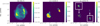 |
Fig. A.2 Same as Fig. A.1 for NGC 6153. |
| In the text | |
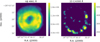 |
Fig. A.3 Same as Fig. A.1 for Hf 2-2, without [C I] 8727 Å. |
| In the text | |
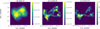 |
Fig. A.4 Same as Fig. A.1 for NGC 6778. |
| In the text | |
|
Fig. A.5 M 1-42 emission-line maps of [N II], Hβ, [O I] 6300 Å and [C I] 8727 Å. Numbers 1 to 5 denote the different LISs aligned along the major axis of the PN. |
| In the text | |
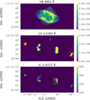 |
Fig. A.6 Same as Fig. A.1 for NGC 7009. |
| In the text | |
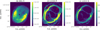 |
Fig. A.7 Same as Fig. A.1 for NGC 3132. |
| In the text | |
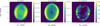 |
Fig. A.8 Same as Fig. A.1 for IC 418. |
| In the text | |
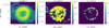 |
Fig. A.9 Same as Fig. A.1 for NGC 6369. |
| In the text | |
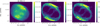 |
Fig. A.10 Same as Fig. A.1 for NGC 6563. |
| In the text | |
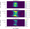 |
Fig. A.11 Same as Fig. A.1 for IC 4406. |
| In the text | |
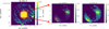 |
Fig. A.12 Same as Fig. A.1 for Tc 1. |
| In the text | |
|
Fig. B.1 The spectrum of two nebular structures (N and S clumps) in NGC 3242. The [Cl II] 8578 Å, [Fe II] 8617 Å and [C I] 8727 Å emissions lines are indicated with blue, orange and green vertical dot lines, respectively. H I 8598 Å and 8665 Å, He I 8649 Å and 8733 Å emissions are also present in the plot. The number in the top left corner indicates the scaling factor applied in the y-axis values. |
| In the text | |
|
Fig. B.2 The spectrum of two nebular structures (N and S clumps) in NGC 3242 covering the wavelength range from 7350 to 7400 Å. The [Ni II] 7378 A emission line is indicated with blue vertical dot line. The number in the top left corner indicates the scaling factor applied in the y-axis values. |
| In the text | |
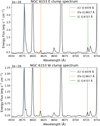 |
Fig. B.3 Same as Fig. B.1 for NGC 6153. |
| In the text | |
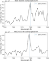 |
Fig. B.4 Same as Fig. B.2 for NGC 6153. |
| In the text | |
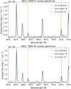 |
Fig. B.5 Same as Fig. B.1 for NGC 7009. |
| In the text | |
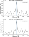 |
Fig. B.6 Same as Fig. B.2 for NGC 7009. |
| In the text | |
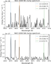 |
Fig. B.7 Same as Fig. B.1 for NGC 6369. |
| In the text | |
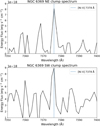 |
Fig. B.8 Same as Fig. B.2 for NGC 6369. |
| In the text | |
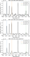 |
Fig. B.9 Same as Fig. B.1 for NGC 3132. |
| In the text | |
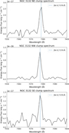 |
Fig. B.10 Same as Fig. B.2 for NGC 3132. |
| In the text | |
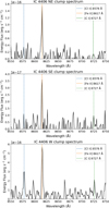 |
Fig. B.11 Same as Fig. B.1 for IC 4406. |
| In the text | |
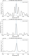 |
Fig. B.12 Same as Fig. B.2 for IC 4406. |
| In the text | |
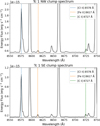 |
Fig. B.13 Same as Fig. B.1 for Tc 1. |
| In the text | |
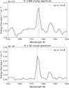 |
Fig. B.14 Same as Fig. B.2 for Tc 1. |
| In the text | |
|
Fig. C.1 Mean confusion matrix for K-Means classifier. |
| In the text | |
|
Fig. C.2 Confusion matrix for KNN classifier. |
| In the text | |
Current usage metrics show cumulative count of Article Views (full-text article views including HTML views, PDF and ePub downloads, according to the available data) and Abstracts Views on Vision4Press platform.
Data correspond to usage on the plateform after 2015. The current usage metrics is available 48-96 hours after online publication and is updated daily on week days.
Initial download of the metrics may take a while.