| Issue |
A&A
Volume 700, August 2025
|
|
|---|---|---|
| Article Number | A269 | |
| Number of page(s) | 14 | |
| Section | Cosmology (including clusters of galaxies) | |
| DOI | https://doi.org/10.1051/0004-6361/202554998 | |
| Published online | 26 August 2025 | |
Quasar pairs as large-scale structure tracers
1
Departamento de Física, Facultad de Ciencias Exactas y Naturales, Universidad de Buenos Aires, Ciudad Universitaria 1428, Pabellón I, Buenos Aires, Argentina
2
Núcleo Cosmo-ufes & Departamento de Física – Universidade Federal do Espírito Santo, 29075-910 Vitória, ES, Brazil
3
Instituto de Astronomía Teórica y Experimental (IATE), CONICET-UNC, Córdoba, Argentina
4
Observatorio Astronómico de Córdoba, UNC, Córdoba, Argentina
5
Comisión Nacional de Actividades Espaciales (CONAE), Córdoba, Argentina
6
Departamento de Física, Universidade Estadual de Londrina, Rod. Celso Garcia Cid, Km 380, 86057-970 Londrina, PR, Brazil
⋆ Corresponding author: This email address is being protected from spambots. You need JavaScript enabled to view it.
Received:
2
April
2025
Accepted:
9
July
2025
Abstract
Aims. Quasars can be used as suitable tracers of the large-scale distribution of galaxies at high redshift given their high luminosity and dedicated surveys. Previous studies have shown that quasars have a bias similar to that of rich groups. Following this argument, quasar pairs could be associated with higher-density environments serving as protocluster proxies.
Methods. In this work, our aim is to characterize close quasar pairs residing in the same halo. This is accomplished by identifying quasar pairs in redshift space. We analyze pair-quasar cross correlations, as well as cosmic microwave background (CMB)-derived lensing convergence profiles centered on quasar and quasar pairs.
Results. We identified quasar pairs in the SDSS-DR16 catalog as objects with relative velocities within |ΔV|≤900 km/s and projected separation less than dp ≤ 2 Mpc, in the redshift range 1.2 ≤ z ≤ 2.8. We computed redshift-space cross-correlation functions using Landy-Szalay estimators for the samples. For the analysis of the correlation between quasars or quasar pairs and the underlying mass distribution, we calculated mean radial profiles of the lensing convergence parameter using CMB data provided by the Planck Collaboration.
Conclusions. We identified 2777 pairs of quasars in the redshift range 1.2–2.8. Quasar pairs show a distribution of relative luminosities that differs from that found in two pairs selected at random with the same redshift distribution, indicating that quasars in these systems distinguish themselves from isolated ones. The cross-correlation between pairs and quasars shows a larger correlation amplitude than the autocorrelation function of quasars, indicating that these systems are more strongly biased with respect to the large-scale mass distribution and reside in more massive halos. This is reinforced by the higher convergence CMB lensing profiles of the pairs compared to isolated quasars with a similar redshift distribution. Our results show that quasar pairs are suitable precursors of present-day clusters of galaxies, in contrast to isolated quasars, which are associated with more moderate density environments.
Key words: galaxies: halos / quasars: general / cosmic background radiation / large-scale structure of Universe
© The Authors 2025
 Open Access article, published by EDP Sciences, under the terms of the Creative Commons Attribution License (https://creativecommons.org/licenses/by/4.0), which permits unrestricted use, distribution, and reproduction in any medium, provided the original work is properly cited.
This article is published in open access under the Subscribe to Open model. This email address is being protected from spambots. You need JavaScript enabled to view it. to support open access publication.
1. Introduction
Studies of the formation and evolution of structures in the Universe have made important recent advances through large galaxy surveys. Among the several new data sets, the Sloan Digital Sky Survey (SDSS) has made major contributions through the identification and redshift measurements of galaxies and quasars, building homogeneous samples suitable for large-scale studies Lyke et al. (2020).
The high luminosity of quasars makes them ideal tracers of structure in the distant Universe, and several studies have analyzed the autocorrelation function in redshift space, which allows for an estimate of the bias of these systems with respect to the mass distribution (Porciani et al. 2004; White et al. 2012, and references therein). The results show that the correlation function amplitude is consistent with rich groups of galaxies, which aligns with expectations from numerical simulation models. In addition, these studies have shown a lack of luminosity dependence of the correlation function on quasar luminosity, which is in contrast to what is found for galaxies, where a strong dependence of clustering amplitude on galaxy luminosity is observed (Zehavi et al. 2011). This independence of clustering strength on quasar luminosity is not surprising, since quasar luminosity is associated with accretion onto the central black hole, a relatively stochastic process that is relatively independent of the global environment of the quasar host, whereas in galaxies, luminosity produced by stars provides a reliable proxy for galaxy mass according to simulations Alberts & Noble (2022).
In this context, exploration of the distribution of quasar systems and their association with mass may shed new light on the joint formation and evolution of quasars and structure. The relatively low number density of quasars allows quasar pairs to be considered as suitable systems for statistical studies, as the number of systems with high membership declines sharply.
In this work, we identify quasar pairs from SDSS DR16 (Lyke et al. 2020) with suitable relative separations and radial velocities. We adopt a maximum projected distance of dp ≤ 2 Mpc and relative velocities within |ΔV|≤900 km/s as reasonable limits for the identification of physical pairs, with a high probability of residing in the same halo. Our final sample of 2777 quasar pairs is suitable for statistical studies involving both the correlation function and cosmic microwave background (CMB) convergence lensing maps. The selection criteria for the quasar samples are detailed in Section 2. The statistical methodologies employed to compute the autocorrelation of the quasar sample are outlined in Section 3. The quasar catalog, specifically for the quasar pairs, is provided in Section 4. Section 5 focuses on the characterization of luminosity and color-color maps. Section 6 presents the cross-correlation functions, while the results pertaining to the studies on CMB convergence lensing are discussed in Section 7.
2. Quasar catalog and subsample
The Sloan Digital Sky Survey (SDSS) is a comprehensive multispectral imaging and spectroscopic redshift survey, utilizing a 2.5-meter wide-angle optical telescope in conjunction with two distinct multi-fiber spectrographs, all situated in New Mexico. One of the most recent catalogs, SDSS DR16, has successfully confirmed the detection of approximately 750 414 quasars, achieved with a spectral resolution of  Lyke et al. (2020). The catalog spans a significant portion of cosmic history, 0 < z < 7.5, and covers approximately 14 555 deg2 of the sky (see Fig. 1). The absolute magnitude in the I band, it spans a large interval, −30 < MI < −23. The SDSS DR16 encompasses three distinct target fields: the Southern Stripe, the Northern Galactic Cap, and the Equatorial Stripe. Each of these areas was selected to maximize survey coverage and provide a comprehensive understanding of the quasar population across the sky Lyke et al. (2020).
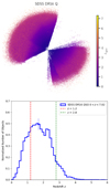 |
Fig. 1. Top panel: Projection of the 3D map representation of quasars from the SDSS DR16Q catalog; the color bar indicates the redshifts of each quasar. Bottom panel: Redshift distribution of the quasars, normalized by the total number of objects in the sample. The median of this distribution is marked by a distinct point for clarity. The subsample within the redshift range z ∈ [1.2, 2.8] is highlighted by vertical lines. |
To enhance the detection of quasar pairs within the SDSS DR16 catalog, we constructed a sample focused on a more restricted redshift window of 1.2 ≤ z ≤ 2.8. The distribution of quasars as a function of the redshift is shown in Fig. 1. The analysis includes 147 325 quasars, which corresponds to approximately 66% of the entire SDSS DR16 catalog1. There are several compelling reasons to focus on the previously mentioned redshift window. We outline a series of justifications grounded in theoretical frameworks and numerical analyses based on various catalogs used in the existing literature. This interval corresponds to a pivotal epoch in the Universe’s history, approximately 10–12 billion years ago-a critical period for unraveling the processes underpinning galaxy formation and the evolution of supermassive black holes (SMBHs). During this period, the Universe underwent significant growth and activity, making it an ideal time to explore the early stages of quasar formation. It was proposed long ago that SMBHs originate from the collapse of massive gas clouds in the early Universe. The energy released during the accretion process plays a crucial role in galaxy evolution, highlighting the importance of feedback mechanisms in regulating star formation within galaxies Silk & Rees (1998).
Subsequently, the connection between black hole mass and the velocity dispersion of the host galaxy bulge-known as the MBH − σ relation-has been essential in showing that black hole growth is closely tied to the evolution of its host bulge. This relationship has been studied extensively in the context of hierarchical galaxy formation models, further illustrating the interconnectedness of these cosmic processes Haehnelt & Kauffmann (2000), Merloni & Heinz (2007). The coevolution of SMBHs and their host galaxies often results from significant mergers between galaxies, which produce feedback that affects both the black hole and the galaxy itself Kormendy & Ho (2013), Harrison et al. (2018).
Using the gravitational lensing effect, where light from a distant quasar is bent by the gravitational field of a foreground galaxy, researchers have greatly improved our understanding of the properties of both quasars and their host galaxies across different epochs, particularly within the redshift range 1 ≤ z ≤ 4.5. Analysis of 31 gravitationally lensed active galactic nuclei (AGNs) and 20 non-lensed AGNs demonstrates the stability of the relationship between black hole mass and luminosity in the R band, represented by the MBH − LR relation, over cosmic time for z ≤ 1.7 Peng et al. (2006).
Additionally, a study of 11 X-ray-selected broad-line AGNs with redshifts from 1 ≤ z ≤ 2 suggested that black holes in the mass range of 108 − 9 M⊙ likely formed before their host galaxies were established Bennert et al. (2011). These findings collectively highlight the complex relationship between SMBHs and their host galaxies, reinforcing the idea that the co-evolution of these systems is deeply interconnected throughout cosmic history Kormendy & Ho (2013), Harrison et al. (2018). Analysis of galaxy formation models that include AGN feedback has shown that quasars are often found in low-mass dark matter halos, typically on the order of 1012 M⊙ Fanidakis et al. (2013). This finding suggests that these environments represent the average conditions in the low-redshift universe (z ≤ 3).
Another important aspect of quasars is how their number density changes with redshift, which is described by the quasar luminosity function (QLF). The QLF measures the number density of quasars per unit of luminosity and is usually expressed as a double power law, featuring a luminosity break, L⋆. This framework distinguishes two scenarios: in luminosity evolution, the luminosity varies over time while the number density remains constant, whereas in density evolution, the number density changes while the luminosity of individual quasars remains stable Richards et al. (2006). Measuring the QLF is crucial for understanding the evolution of SMBHs and for placing constraints on various cosmic backgrounds Ross et al. (2013). A detailed analysis of the QLF was carried out using the SDSS-III DR9 catalog, which includes 22 301 quasars across an area of 2236 deg2. The catalog provides spectroscopic redshift measurements in the range z ∈ [2.2, 3.5] and incorporates K-corrections for accurate luminosity assessments. The results confirmed the double power-law relationship in the range z ∈ [0.3, 2.2]], but also identified a clear break in this relationship around z = 2, with MI(z = 2) = − 24.5. For z ≥ 2.2, they found a log-linear trend in quasar luminosity amplitude and break luminosity Ross et al. (2013).
By combining data from the SDSS and 2dFQSO surveys, researchers examined the clustering properties of quasars up to redshift z = 5, calculating the two-point projected correlation function for quasars within r < 20 h−1 Mpc. Their analysis indicated a halo mass of approximately 1013 M⊙, with a slight increase observed with redshift. Additionally, when considering the fraction of halos hosting active quasars, the typical lifetime of quasars at high redshift (z > 1) is estimated to be around tQ ≃ 108 yr Porciani et al. (2004).
In addition to the previously discussed reasons for selecting a redshift window between 1.2 and 2.8, another significant factor concerns the completeness of the quasar sample Schneider et al. (2003), Pâris et al. (2012), Lyke et al. (2020). The initial releases of the SDSS DRII quasar catalog, which contained only 16 713 objects and covered an area of 1360 deg2 across the redshift interval z ∈ [0.08, 5.41], highlighted the need for completeness in the sample. To achieve reliable identification of quasars, robust selection criteria based on brightness, magnitude, and color, along with multi-color imaging systems, were implemented by the SDSS collaboration. This approach effectively differentiated quasars from stars and galaxies Schneider et al. (2003). Significant improvements were introduced in the SDSS DR12 quasar catalog, which incorporated photometric detections across five bands with a typical accuracy of 0.03 mag, as well as spectroscopic redshift measurements obtained by analyzing strong emission lines from carbon and magnesium Pâris et al. (2012). The deep-scan capabilities of the survey allowed it to reach specific magnitude thresholds, ensuring that quasars at higher redshifts (z > 2.1) remained detectable and leading to the discovery of 297 301 quasars over 9376 deg2. Spectroscopic follow-up was conducted after the initial photometric identification, confirming both the quasar nature and the redshift measurements. The expanded survey volume increased the likelihood of finding quasars, thereby improving the completeness of the sample Pâris et al. (2012). These elements and analyses collectively contribute to a better understanding of the completeness and potential selection effects that may influence the observed distribution of quasars. For example, the typical completeness value for quasars in the SDSS DR16 catalog is approximately 99.8%, with a contamination rate below 1.3% Lyke et al. (2020). In summary, we began our analysis in the redshift range [2.2, 2.8], where the SDSS DR16 catalog is reasonably complete. We then extended our study to lower redshifts, starting at z = 1.2. This choice provides a broader perspective, as the catalog becomes increasingly incomplete at redshifts above 2.8. Our main goal is to investigate how redshift evolution unfolds within this context. This redshift range is also adopted in other observational studies. At cosmic noon, a cross-match between Gaia EDR3 and SDSS DR16 data enabled the detection of quasar pairs with angular separations between 0.3″ to 3″ at redshifts greater than 1.5 (cf. Chen et al. (2023) and reference therein). Additionally, the joint analysis of the James Webb Space Telescope/Near-Infrared Spectrograph integral field unit and Gaia identification led to the discovery of an SMBH pair at a redshift of z = 2.17, separated by 3.8 kpc Ishikawa et al. (2025).
3. Two-point correlation function analysis for the subsample
The gravitational processes that dictate the formation and evolution of cosmic structures are elegantly encoded in the correlation function of galaxies. Moreover, the correlation function of quasar distributions plays a crucial role, since quasars serve as exceptional tracers of large-scale structures, particularly at high redshifts (z > 1) Shen et al. (2009), Laurent et al. (2017). Their unique properties allow exploration of the gravitational dynamics that govern the evolution of the Universe, providing valuable insights that complement the analyses of galaxy clustering Song et al. (2016).
We began our investigation with an exploratory analysis of the data drawn from the SDSS DR16 catalog Lyke et al. (2020). We applied a series of cuts based on the absolute magnitude in the I band across the sample. Data are represented according to the relationship |M|I(z) = |M|0 + 1.8(z − 0.8), where |M|0 ∈ [|M|min, |M|max]. Here, the lower and upper limits of each band are defined as |M|min = 18 + n, |M|max = |M|min + 1, where 1 ≤ n ≤ 10 (see Fig. 2). This methodology enables us to identify any gradients present in the quasar data, which is crucial for the subsequent construction of the (weighted) random data set.
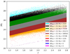 |
Fig. 2. Absolute magnitude across the redshift range. The magnitude bands are defined according to the relationship |M|I(z) = |M|0 + 1.8(z − 0.8). |
Next, we carried out numerical computation of the two-point correlation function (2PCF), using the capabilities of the corrfunc package Sinha & Garrison (2020). The corrfunc package2 enabled us to investigate the intricacies of the correlation function, specifically by examining the autocorrelation properties and the coherence length associated with our selected subsample. Through this analysis, we aimed to elucidate the power-law behavior that emerges within the linear regime White et al. (2012). To facilitate this exploration, we began by constructing a random catalog that mirrors the redshift interval of our original data set. The random catalog served as a crucial reference point, enabling us to compare the observed correlations with those expected from a uniformly distributed sample.
For a resolution of Nside = 32, we constructed a mask to accurately mimic the distribution of quasars across the celestial sphere. To achieve this, we used the Healpix package3 Górski et al. (2005), where Nside = 32 is represented by 12 288 pixels. The procedure was as follows. We constructed a smoothed and weighted map designed for quasars to populate the random catalog, accounting for the gradient in the data Lyke et al. (2020). The latter smoothed map serves as a probability density function (PDF). The process began by generating random right ascension (RA) and declination (Dec) coordinates. We then checked the compatibility of these random coordinates with the smoothed map. We also ensured that each point fell within the designated mask; thus, points are more likely to be accepted into the random catalog if they are generated in regions with a high density of quasars. We evaluated the probability of the normalized weighted map at these coordinates and compared it with a randomly generated filter value between 0 and 1. If the filter value exceeded the probability at the selected RA and Dec coordinates, the process was restarted from the previous step. Otherwise, we accepted and saved the random RA and Dec. The key aspect of our approach was the use of a probabilistic map instead of computing a PDF. In doing so, we ensured that the random RA and Dec points were concentrated in areas where quasars are more prevalent, resulting in a catalog that accurately reflects the spatial distribution of the original dataset. In Fig. 3, we present the distribution of quasars across the celestial sphere alongside its corresponding mask based on this procedure. We also verified that the distribution of the random data in redshift mirrored the trends observed in the original data sample. The comparison ensured that our randomization process preserves the underlying characteristics of the redshift distribution, allowing a confident assessment of the significance of our findings.
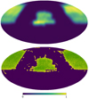 |
Fig. 3. Top panel: Mask used to generate a random map at a resolution of Nside = 32, incorporating a smoothing factor of θs = 4°. Bottom panel: The yellow region represents the dataset points, while the green region highlights the random points generated using the probability density function alongside the smoothing mask. The overlap between both sets indicates a strong level of concordance. |
To compute the correlation function in the redshift space using the corrfunc package Sinha & Garrison (2020), we used the Landy-Szalay estimator Landy & Szalay (1993), which provides minimal variance,
 (1)
(1)
where DD denotes the number of distinct data pairs, RR the number of different random pairs, and DR is the number of cross-pairs between the real and random catalogs within the same distance bin. The estimator Landy-Szalay Landy & Szalay (1993) proved advantageous because it effectively managed edge effects, allowing appropriate consideration of missing data beyond the sampled region, which may have irregular boundaries. In Fig. 4, we show the 2PCF obtained using the previously constructed random set.
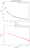 |
Fig. 4. Top panel: Two-point correlation function obtained using the LS estimator for the total sample, z ∈ [1.2, 2.8]. Red point represents the correlation function with its error bars. Bottom panel: The dashed red curve indicates the best linear fit in logarithm scale. In the linear regime, the correlation function can be parametrized as ξ(s) = (s/s0)−γ with γ = 1.21 ± 0.03 and s0 = 12.25 ± 1.30. |
We applied the Bootstrap method to estimate errors directly from the calculated correlation function Norberg et al. (2009), Mohammad & Percival (2022). Specifically, we divided the survey into Ns subsamples and performed a random resampling with replacement to create Ns bootstrap samples. For each bootstrap sample, we computed the correlation function based on the resampled data. The covariance matrix Cij between two estimates ξi and ξj at different bin values si and sj is given by Norberg et al. (2009), Mohammad & Percival (2022)
 (2)
(2)
where  is the estimate of the correlation function at bin si from the k-th bootstrap sample, while ⟨ξj⟩ denotes the mean estimate across all the bootstrap samples, defined as
  . In this analysis, we considered Ns = 100, and the number of bins in the s−variable was 60. We also performed a linear regression analysis using the estimated correlation function along with its corresponding bootstrap errors. We required that the convergence condition
  hold. In the linear regime, the correlation function can be expressed as a power law given by ξ = (s/s0)−γ. Our linear fit results in an exponent index of γ = 1.21 ± 0.03 and a correlation length in the redshift space of s0 = (12.25 ± 1.30) Mpc/h for a determination coefficient of R2 ≃ 0.98. The values obtained agree with existing literature on quasars at intermediate redshifts White et al. (2012). It is important to note that the correlation maintains physical significance for s < 30 Mpc h−1, beyond which it tends to diminish toward zero. Our analysis demonstrates that the correlation functions for the different magnitude subsets remain largely consistent in their values of γ and s0.
4. Quasar pair catalog
We outline the primary criteria used to identify quasar pairs within the subsample at redshifts 1.2 ≤ z ≤ 2.8 extracted from the SDSS DR16 catalog Lyke et al. (2020). The identification of these quasar pairs through spectroscopic measurements requires a series of physically reasonable assumptions. To remain consistent with the limitation of the SDSS DR16 sample4, we propose that a pair of quasars must have the following features:
-
The quasar pairs must adhere to a limiting velocity constraint such that |ΔV| = c(z2 − z1) ≤ 900 km/s.
-
The members of each pair should be in close proximity, specifically with a projected distance of dp ≤ 2 Mpc.
These two conditions together define the cylindrical volume within which the quasar pairs are located. In addition, within any given pair, one quasar is expected to exhibit higher luminosity, reflected by a smaller (and thus more negative) apparent magnitude, mi. The method developed to identify these quasar pairs can be summarized as follows. Each quasar in the catalog is assigned a unique ID number along with all its physical properties, including angular coordinates (RA, Dec), redshift, apparent magnitude, and luminosity expressed in solar units. We adopted the Planck 2018 background as a fiducial cosmology for numerical computations with the Astropy package5 Astropy Collaboration (2013). The angular diameter distance for each quasar was calculated based on its redshift and the Planck 2018 cosmology. The subtended angle, in radians, was determined from a specified maximum distance and subsequently converted to degrees. The RA and Dec coordinates were translated into Healpix/Healpy6 pixel indices for spatial analysis Górski et al. (2005). Each pixel corresponds to a specific location on the celestial sphere, and we employed a high resolution of Nside = 2048. We stored the vectors for each pixel for future use in the query-disk routine and created a list to keep track of neighboring pixels. For each quasar, neighboring pixels within a defined angular distance were identified, facilitating the analysis of local quasar environments. The radius in radians was computed using the angular distance, and the neighboring pixels within the specified disk were recorded. The algorithm then searched for nearby quasar pairs based on their redshift and angular distance, ensuring that no pair was identical and that pairs lie within a predetermined redshift tolerance. Duplicate pairs were filtered using ordered tuples, retaining only the closest pairs constrained by a physical distance criterion of dp ≤ 2 Mpc.
The distribution of identified quasar pairs is shown in Fig. 5. The SDSS DR16 catalog, with redshifts ranging from z = 0.0007 to z = 7.023, contains a total of 4011 identified quasar pairs. Most quasar pairs are found in the first two redshift bins, z ∈ [0.0007, 1.2] and z ∈ [1.2, 2.8], with additional pairs detected beyond z = 4.4. The highest detection rate occurs in the second redshift interval z ∈ [1.2, 2.8], which represents 2777 pairs; this is the sample on which we focus our study. The histogram of projected distances (in Mpc) for all 2777 quasar pairs is also shown in Fig. 5. The average distance between pairs is d = (0.986 ± 0.5009) Mpc, and only 21 pairs have projected separations below the minimum projected distance resolved by SDSS,  . Overall, the peak of the histogram suggests that quasar pairs tend to cluster around this average projected distance.
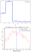 |
Fig. 5. Top panel: Distribution of quasar pairs across the complete redshift window of the SDSS DR16 quasar catalog. The highest concentration of pairs is found within the redshift range z ∈ [1.2, 2.8], totaling 2777 pairs. The catalog contains a total of 4011 pairs. Bottom panel: Distribution of quasar pairs detected within a cylindrical volume characterized by a projected radius of dp ≤ 2 Mpc and a length of |ΔV| = 900 km/s. Black vertical lines denote |

We also examined various bounds of |ΔV| to investigate how the number of pairs detected changes as this condition is relaxed within the redshift interval z ∈ [1.2, 2.8]. For the condition |ΔV|≤600 km/s, the number of pairs detected decreases to 1915, representing 39% of the total. In contrast, when considering |ΔV|≤1200 km/s, the number of pairs detected increases to 3605, which represents 73% of the entire subsample. Consequently, we focus on the most conservative case moving forward, which corresponds to |ΔV|≤900 km/s. The distribution of quasar pairs within the RA-Dec plane is illustrated in Fig. 6 for the conservative scenario.
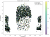 |
Fig. 6. Scatter plot of the 2777 quasar pairs that satisfy the criterion |ΔV|≤900 km/s. The color bar, normalized across the dataset, represents the redshift variation, Δz, between quasar pairs, effectively conveying this continuous variable through a color scale. |
We next addressed an additional observational point regarding the detection of quasar pairs. A fundamental question was whether the SDSS camera is capable of effectively resolving two quasars that constitute a confirmed pair. This question was essential for understanding the limitations of observational data and the ability of the SDSS to distinguish quasar pairs, which is crucial for accurate pair identification and subsequent analysis. To answer this, we adopted a conservative angular resolution for the SDSS telescope Lyke et al. (2020), with θ ≥ θSDSS = 5″, along with a mean redshift value of zmean = 2.4. The physical distance corresponding to the SDSS angular resolution is approximately  (cf. Fig. 5). This result is significant given previous observations indicating that the distribution of distances between quasar pairs is around d = 0.986 Mpc. Thus, we conclude that the SDSS camera is capable of resolving these objects.
Another important question is whether the quasar pair sample might be contaminated. For example, background galaxies can create multiple images of a single quasar, making it difficult to identify true quasar pairs. To address this issue, we reassessed the quasar pair sample by focusing only on pairs with  , where
  is the error in the spectroscopic measurements from the SDSS DR16 catalog Lyke et al. (2020) and ΔV = c(z2 − z1). Our analysis revealed that out of the 2777 detected quasar pairs, only 9.9% were potentially contaminated. To further investigate these cases, we used the specific coordinates of these quasars to examine their corresponding spectra from the SDSS DR16 catalog. However, the SDSS DR16Q catalog has already addressed several contamination issues within the entire sample, including duplicity due to the observational strategy, reporting a contamination rate of up to 1.3% Lyke et al. (2020). Our criteria for assessing contamination were as follows. If both quasars in a pair exhibited identical features in their spectra, this suggested that they could be duplicate images of the same quasar, influenced by foreground galaxies. Conversely, if the elements of a quasar pair displayed different amplitudes and positions of their emission lines, we concluded that they were not multiple images of the same object. The position of each object in the sky and its spectrum can be accessed through the SkyServer DR16 website7.
Using the SkyServer DR16 interface, we obtained the spectra associated with each quasar by inputting their angular coordinates on the sky. After normalizing each spectrum to itsmaximum value, we set the criterion that if the spectra of quasar pairs differed by less than 5%, they could be considered as a single quasar producing multiple images, especially if the redshifts of the component quasars were very close. To analyze the spectral lines and their ratios, we employed the PyQSOFit package Guo et al. (2019). For pairs where 0 < ΔV ≤ 60 km/s, we determined that only 30% could be the same lensed object. For our total sample of 2777 pairs, we expect a contamination of less than 3.5% due to lensing effects, which corresponds to 66 cases. A similar approach was used to create a new quasar pair catalog based on the DESI DR1 quasar sample, leading to the identification of 1842 new pairs by applying a projected separation criterion of dp ≤ 110 kpc and a radial velocity difference limit of ΔV ≤ 600 km/s. This method not only improves the completeness of the quasar pair sample but also helps ensure a more accurate identification of real pairs, thereby reducing the potential contamination from background sources Jing et al. (2025).
To further characterize the catalog of quasar pairs, we performed a numerical estimation of the comoving number density of quasars and quasar pairs within the redshift interval [1.2, 2.8]. The surveyed sky fraction is approximately 0.65%, covering 26 732 deg2, leading to a numerical (comoving) density of nq ≃ 5.8 × 10⁻⁸ Mpc−3. This value aligns well with the findings reported in Croom et al. (2005), which quotenq ≃ 8.2 × 10⁻⁹ Mpc−3. Considering a minor sky fraction for the quasar pairs, fsky, pair = 0.54, we observe a notable reduction in the estimated numerical (comoving) density of these pairs. This yields approximately npair ≃ 2.4 × 10⁻¹⁰ Mpc−3. This finding highlights the significant influence of observing a restricted sky area, combined with a relatively small sample of detected pairs, on the estimated density of quasar pairs, particularly in contrast to the densities associated with individual quasarsCroom et al. (2005).
5. Luminosities and color-color maps
In this section, we explore whether quasar pairs exhibit particular properties compared to quasars in isolation. We focus on the luminosity of the quasar pairs Wu & Shen (2022), as well as the luminosity ratio of the pair members.
Quasar luminosities must account for the K-correction Ross et al. (2013). Our approach follows Lyke et al. (2020), using a pre-calibrated K-correction table from Richards et al. (2006). The K-corrected absolute magnitude in the I band was calculated using the relation
 (3)
(3)
where mI, ap is the apparent magnitude, MI, abs is the absolute magnitude in the I band, DM(z) - log10[DL(z)/10pc] is the distance modulus, and A(z) represents extinction. The K-correction, represented in the second to last term of the equation, can be specified at z = 2 as detailed in Appendix B of Ross et al. (2013). Our method for integrating the K-correction closely follows the procedures outlined in Ross et al. (2013) and Lyke et al. (2020). We used the Planck 2018 fiducial cosmology for distance calculations. The absolute magnitude MI, abs for a given quasar was obtained by correcting the apparent magnitude for extinction, distance modulus, and K-correction. Apparent magnitudes in the I band were taken from the PSFMAG column in the FITS file of the SDSS DR16 QSO catalog Lyke et al. (2020)8. K-corrections were obtained using data from Richards et al.’s table, which is limited to a specific redshift range Richards et al. (2006). For each redshift z, we selected the closest entry in the K-correction table to extract the corresponding K-correction value. This process allowed us to calculate the corrected absolute magnitude MI, abs for each quasar. Once we had MI, abs, we converted it to luminosity in the I band in solar units using
 (4)
(4)
where L⊙ is the solar luminosity and MI, ⊙ is the absolute magnitude of the Sun in the I band. Thus, we obtained reliable estimates of the luminosities in the I band, allowing further analysis of quasar in pairs and in isolation. In Fig. 7, we display the distribution of luminosities, showing that L = (1.75 ± 0.52)×1016 L⊙.
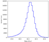 |
Fig. 7. Histogram of the quasar luminosity distribution after applying K-corrections. The horizontal axis is displayed on a logarithmic scale. |
It is now well understood that galaxy evolution, shaped by AGN feedback, often leads to quasars residing in low-mass dark matter halos Fanidakis et al. (2013). Furthermore, the number density of quasars per unit luminosity follows a double power-law relationship within the redshift range z ∈ [0.3, 2.2], while showing log-linear behavior for z ≥ 2.2 Ross et al. (2013). This suggests that quasar pairs-acting as proxies for protoclusters Muldrew et al. (2015), Alberts & Noble (2022)-may share similarities owing to their common dark matter halo.
Here, we aim to address whether quasar pairs within the same dark matter halo represent a distinct class of objects, rather than representing a simple combination of two individual quasars from the sample. To address this point, we examine the distribution of luminosity ratios, L1/L2, for quasar pairs, where L1 and L2 correspond to the smaller and larger luminosities, respectively. This analysis allowed us to investigate the intrinsic relationships between the luminosities of these unique objects, offering insights into their relative behaviors. Additionally, we generated 100 random sets of control pairs derived from the isolated quasar set. These ensembles do not satisfy the typical constraints of ΔV ≤ 900 km/s and dp ≤ 2 Mpc9. This approach provided a baseline for comparison, which is essential for understanding the characteristics of the quasar pairs and their luminosity distributions relative to those of the control pairs. By contrasting the observational data with these control constructs, we aimed to identify any significant patterns or anomalies that may arise, thereby enriching our comprehension of these astrophysical entities.
We constructed the control pair sample by imposing that the angular separation between the two objects exceeded 5.7° (1 radian), and restricted the maximum allowed redshift difference to Δz ≤ 0.003. We also verified that the histograms of Δz for the true pairs and control pairs were quite similar. This consistency in distribution ensured that there were no significant differences in the redshift differences between the two groups, indicating that the selection criteria for both the true and control pairs were comparable. We generated 500 sets of control pairs, each containing the same number of detected pairs, resulting in 615 control pairs per set. We focused on assembling the new set using a random algorithm to avoid any selection bias10.
Figure 8 illustrates the differences between the true quasar pairs and the control pairs. The mean luminosity ratio of L1/L2 shows significant variations between these two datasets. When calculating the fraction of real pairs satisfying the condition Ftrue pair(L1/L2 > 0.75), and comparing it to the corresponding fraction for the control pairs, Fcontrol pair(L1/L2 > 0.75), we can define the ratio of these fractions as ℛ = Fpair/Fcontrol pair. The purpose of calculating Fcontrol pair(L1/L2 > 0.75) was to determine whether the control pairs can mimic the histogram of quasar pairs with L1/L2 > 0.75.
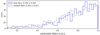 |
Fig. 8. Distribution of luminosity ratios for true quasar pairs and control pairs. The true quasar pairs are indicated in blue, while the control pairs are shown in gray. |
The results show that ℛ > 1, indicating that the two sets of pairs have fundamentally different properties, likely reflecting different accretion mechanisms that affect the luminosity ratios L1/L2. Our analysis finds that 62.32% of true pairs exhibit L1/L2 > 0.75, while only 57.56% of control pairs meet this criterion. Thus, the calculated value of ℛ = 1.08 indicates that true pairs are more likely to show a luminosity ratio L1/L2 > 0.75 compared to their control sample counterpart. Moreover, our findings are consistent across all 500 control datasets, each containing 615 pairs, reinforcing the robustness of our conclusions.
Another approach to investigate the validity of random-generated data sets compared to true pairs is to analyze the behavior of the total luminosity of the pair, i.e., the sum of the member luminosities. This is motivated by the possibility of a different behavior for quasars in association relative to randomly selected objects (noting that the results from the luminosity ratio analysis could imply that both quasars in a pair have either low or high luminosities).
As shown in Fig. 9, the distribution of the logarithm of summed luminosities differs between true pairs and control pairs. The histogram for true pairs exhibits a narrower spread around its mean, indicating that these pairs are more closely clustered in terms of their luminosity ratios. In contrast, the histogram for the control pairs exhibits a broader spread, indicating a larger luminosity variability among them. This difference in distribution reinforces the notion that true pairs are more consistent in their luminosity characteristics, whereas control sample pairs tend to display a wider range of luminosity ratios.
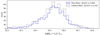 |
Fig. 9. Distribution of the logarithm of the sum of luminosities for true quasar pairs and control pairs. True quasar pairs are shown in blue, while control pairs are shown in gray. |
Our analysis reveals a significant difference between the two datasets, suggesting that the mechanisms driving the luminosity characteristics of quasars in association are intrinsically distinct. These differences may largely arise from the co-evolution of quasars with their surrounding environments, which influences their accretion processes and, consequently, their luminosity profiles Porciani et al. (2004). Such interactions with the environment can significantly shape the properties of quasars, leading to observable variations in luminosity distributions Eftekharzadeh et al. (2015).
Next, we attempted to further quantify the differences observed between true quasar pairs and their control counterparts. Our main goal was to evaluate whether a modified set of pairs from the control sample, hereafter referred to as “simulated” quasar pairs, could effectively approximate the real data. In this approach, we focused on the tercile of the control sample associated with the less luminous quasar and increased its luminosity by 30%.
Figure 10 shows that this procedure creates a simulated quasar pair sample with a distribution of luminosity ratios L1/L2 that closely resembles the actual data, highlighting the strength of the similarity effect.
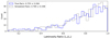 |
Fig. 10. Distribution of luminosity ratios for true quasar pairs and simulated pairs is illustrated. True quasar pairs are shown in blue, while simulated pairs are shown in gray. |
Fundamentally, this observation indicates that true pairs exhibit closely similar luminosity values. In contrast, control pairs show a more pronounced disparity between their most luminous and least luminous members. This distinction reinforces the hypothesis of a common cosmic evolution of our pair sample.
In the final stage of characterizing the quasar pairs, we performed a comparative analysis of their color-color map against that of the entire selected sample. As illustrated in Fig. 11, the color-color map derived from the PSF magnitudes in the g, i, r, and z bands for the complete subsample reveals a range of values given by −6.04 ≤ (g − r)≤5.64 and −3.68 ≤ (r − z)≤7.15 Lyke et al. (2020). However, for the detected quasar pairs, these maximum and minimum values are significantly constrained to −1.55 ≤ (g − r)≤2.21 and −1.17 ≤ (r − z)≤2.53. Notably, 90% of the data points associated with the quasar pairs fall within the interval (r − z)×(g − r)∈[−0.10, 0.85]×[−0.17, 0.42]. These results indicate older stellar populations or dust effects, along with the possibility that bluer colors signify ongoing star formation. This is consistent with the current understanding of quasar environments and their host galaxies Kauffmann & Heckman (2009). For 90% of the detected quasar pairs, we obtain (i − z)×(r − i)∈[−0.06, 0.69]×[−0.13, 0.30]. Again, the negative minimum values suggest the presence of younger, hotter stars, while the positive maximum values indicate the influence of older stars or dust obscuration. These interpretations are well supported within the framework of quasar studies Richards et al. (2006). Different sequences of color-color maps are displayed in Fig. 12
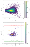 |
Fig. 11. Top panel: Color-color map for the entire subsample of quasars. Bottom panel: Color-color map for the detected quasar pairs. Here, log(N) represents the logarithm of the number of quasar pairs within each region of the color-color map. Note that in some cases, the maximum or minimum values may lie outside the displayed data range. |
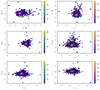 |
Fig. 12. Different color-color maps for the quasar pairs. |
6. Cross-correlation of quasar pairs
We broadened our investigation by analyzing the cross-correlation between quasar pairs and individual quasars. The rationale for examining the cross-correlation is that within a defined redshift range, quasars act as tracers of mass distribution, albeit with an inherent bias. Consequently, we analyzed the clustering behavior of quasar pairs relative to the underlying background represented by the quasar sample not included in these pairs. This approach deepens our understanding of the large-scale structure of the Universe and refines our mapping of the cosmic web, especially as these entities engage and coexist with galaxies in the vast Universe Menard & Bartelmann (2002).
To ensure that the identified pairs are physical composite objects located within the same dark matter halo and likely experiencing similar accretion processes – rather than being merely coincidental nearby quasars – we implemented a series of verification tests. Among these, we conducted an analysis of the cross-correlation of signals between the quasar sample and the corresponding subsample of pairs, as stated previously. We followed the same protocol as before. Using the corrfunc package Sinha & Garrison (2020), we calculated ξ(s, μ), subsequently converting this to the number of pairs using the convert-3d-counts-to-cf routine. This enabled us to derive the Landy & Szalay (1993) estimator for the cross-correlation,
 (5)
(5)
where Dq represents the set of quasars in the subsample, and Dp denotes the dataset of the quasar pairs, using the mid-vector between the two quasars to represent each pair. We generated an associated random set that satisfied the specifications outlined in the corrfunc manual Sinha (2013). Specifically, we ensured that the size of the random set and the data set was consistent with the relationship N(Rp) = 3N(Dp). The latter approach improved statistical robustness and mitigated any potential biases in our correlation measurements. We integrated the previous method with a bootstrap algorithm Mohammad & Percival (2022). By applying the bootstrap technique, we derived confidence intervals and improved the robustness of our cross-correlation analysis. This iterative process allowed us to quantify the uncertainties associated with our measurements, ultimately enhancing the statistical significance of our findings. We considered one bin in the μ-variable with μmax = 1 Sinha (2013) and 60 bins in the separation s-variable. The resampling number employed in the bootstrap method11 was set to Nrs = 10012, consistent with the approach outlined in Mohammad & Percival (2022).
We aimed to illustrate the overall behavior of the cross-correlation amplitude across the entire redshift range of interest, 1.2 ≤ z ≤ 2.8. We subsequently revisited this cross-correlation function under various scenarios, which involved adjusting the redshift bins and exploring different combinations of cuts based on L1/L2 and log10(L1 + L2)/L⊙. These cuts are well-founded, as supported by the luminosity analysis of quasar pairs presented in Section 5.
In Figure 13, we present the cross-correlation function for this specified interval, comparing its signal to both the autocorrelation of all quasars and that of isolated quasars–those not associated with any pairs. Our analysis indicates that the cross-correlation between pairs and isolated quasars does not produce a stronger signal than the overall cross-correlation derived from the complete sample within this interval. We observe that the cross-correlation signal between pairs and quasars consistently surpasses the autocorrelation signal of quasars by a significant margin. The signal is clearly stronger than the autocorrelation for separations of s < 25 Mpc h−1. While both correlation signals exhibit a similar decline at larger separations, as illustrated in the log-log plot in Fig. 13, the correlation scale for quasar pair correlations is approximately s0, pq ≃ 21.41, nearly doubling the correlation length of the quasar sample, which is s0, qq ≃ 12.25. This observation indicates that quasar pairs within this range demonstrate significant clustering, implying a stronger spatial association influenced by underlying physical processes. Such clustering is one reason why quasar pairs can be regarded as proxies for protoclusters Muldrew et al. (2015), Alberts & Noble (2022).
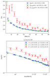 |
Fig. 13. Top panel: Comparison of the two-point cross-correlation function, derived using the LS estimator between quasar pairs and individual quasars within the 1.2 ≤ z ≤ 2.8 redshift window. The cross-correlation is shown alongside autocorrelation for the full sample in that interval and for isolated quasars. Bottom panel: Linear regressions for the three cases are depicted on a logarithmic scale to visualize their slopes. The estimates of (γ, s0) remain consistent across all three cases. |
We now focus on the cross-correlation function on different scales, 2.2 ≤ z ≤ 2.8 (cf. Fig. 14). The analysis reveals that the cross-correlation signal is considerably stronger for separations s < 20 Mpc h−1. In other words, quasar pairs within this range exhibit a more significant clustering tendency, suggesting a closer spatial relationship among these objects. The cross-correlation function of quasar pairs with quasars is found to be 5.98 times higher than the autocorrelation function of quasars when considering separations s < 20 Mpc h−1. At large separations, both signals exhibit a similar decline, demonstrating a consistent behavior in the correlation functions. To gain insight into how the correlation length for the cross-correlation of quasar pairs with quasars compares to the quasar-quasar case, we observe that the condition ξpq(s0, pq) = 1 corresponds to a scale of approximately s0, pq ≃ 18.94. In contrast, for the autocorrelation case, where ξqq(s0, qq) = 1, the scale is around s0, qq ≃ 9.64. Visual examination indicates a significant difference in correlation lengths between these two scenarios, highlighting the influence of the cross-correlation on the spatial distribution of quasar pairs13. As expected, the correlation length of the quasar pairs is greater than that of individual quasars.
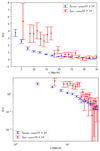 |
Fig. 14. Top panel: Two-point cross-correlation function obtained using the LS estimator between quasar pairs and individual quasars at intermediate redshift. The 2PCF for the entire sample, computed using a bootstrap method for resampling, is also included. Bottom panel: The same 2PCF functions are shown on logarithmic scales. |
We explored the implications of excluding quasar pairs from our sample and focused solely on the two-point correlation function derived from the modified dataset (autocorrelation). This allowed us to better understand the characteristics and clustering behavior of the remaining quasars. The signal maintains a low level, similar to that observed in the full sample. Specifically, within the linear regime, we find the power-law parameters to be s0 = (10.84 ± 1.99) Mpc} h−1 and the exponent is γ = (1.36 ± 0.06). These results are consistent with our previous findings, reinforcing the robustness of our analysis.
Another important aspect is the impact of splitting the subsample in the redshift range 2.2 ≤ z ≤ 2.8 into two smaller subsets: 2.2 ≤ z ≤ 2.5 and 2.5 ≤ z ≤ 2.8. This partition allowed us to investigate potential differences in clustering behavior and correlation properties between these two redshift intervals, providing a clearer understanding of how the quasar pair distribution evolves with redshift. For brevity, we present the correlation functions for the redshift range 2.2 ≤ z ≤ 2.5, as these results are sufficient to support our conclusions. Examining the cross-correlation reveals notable variability in the residuals correlating with the level of the independent variable. We conclude that the assumption of constant variance does not hold, as confirmed using the Breusch-Pagan algorithm. To address this, we performed a weighted linear regression analysis. A weight coefficient of  is obtained, along with the following parameter estimates: γ = 2.77 ± 0.44 and s0 = (16.27 ± 3.27) Mpc h−114. Overall, we find that the cross-correlation function of quasar pairs with quasars exhibits a significantly stronger signal compared to both the isolated case (quasars not belonging to pairs) and the standard quasar-quasar correlation. The difference is visually apparent in Fig. 15, where the enhanced clustering signal of the cross-correlation is clearly discernible.
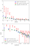 |
Fig. 15. Top panel: Two-point correlation function derived using the LS estimator for the cross-correlation between quasar pairs and individual quasars within the redshift interval 2.2 ≤ z ≤ 2.5. The 2PCF for the entire subsample is included, computed using the resampling bootstrap method, as well as the 2PCF for isolated quasars not belonging to any pair. Bottom panel: The same 2PCFs are presented on a logarithmic scale. |
We suggest an alternative approach to validate that the observed cross-correlation is physically significant and not merely a consequence of the chosen redshift bins. This involves partitioning the original subsample within the redshift window z ∈ [2.2, 2.8] into two distinct datasets by applying a cutoff on the logarithm of the sum of the luminosities. By adopting this approach, we further assess whether our results maintain physical relevance across different partitions, using the luminosities of the quasar pairs as input. Figure 16 shows that the cross-correlation signal persists regardless of the cutoff or partitioning method employed. Although the error bars may appear larger, even with the same bootstrap method applied, this increase is primarily associated with the reduced sample size after partitioning based on the criterion log10(L1 + L2)/L⊙ ≶ 14.548. This observation underscores the resilience of the correlation across different approaches, reinforcing the validity of our findings despite variations in data partitioning. As anticipated, linear regression may be less reliable in certain scenarios. For the case where log10(L1 + L2)/L⊙ > 14.548, the slope is found to be γ = (2.00 ± 0.40) and the correlation length is s0 = (16.00 ± 1.70), with a coefficient of determination R2 ≃ 0.80. In contrast, for the opposite case where log10(L1 + L2)/L⊙ ≤ 14.548, the estimations yield γ = (2.00 ± 0.63), s0 = (16.00 ± 4.15), and R2 ≃ 0.68.
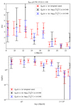 |
Fig. 16. Top panel: Comparison of two-point cross-correlation functions obtained using the LS estimator between quasar pairs and individual quasars in the 2.2 ≤ z ≤ 2.8 redshift window, shown with different partition criteria. Bottom panel: The same two-point cross-correlation functions are displayed on logarithmic scales to visualize their slopes. |
These findings warrant further exploration, which we undertake in the next section through an investigation of the convergence CMB lensing signal 7. Additionally, we will assess whether the amplitude of the convergence signal is primarily influenced by the more luminous or the less luminous quasar pairs.
7. CMB lensing signal
In this section, we examine the association of mass with quasars and quasar pairs using CMB κ convergence maps. Given previous results and the fact that the hosts of quasars are galaxies, we expect a higher κ convergence signal in the neighborhood of quasar pairs compared to the vicinity of isolated quasars. Previous studies for similar samples have shown a lensing signal at κ ∼ 2 ⋅ 103 at angular distances below one degree Geach et al. (2019), Petter et al. (2022), Eltvedt et al. (2024). Taking this into account, we followed the methodology of Toscano et al. (2023) and calculated radial convergence profiles using the CMB data products released in 2018 by the Planck Collaboration Planck Collaboration VIII (2020). We reconstructed the map from the spherical harmonic coefficients kLM15, using all available L values e (LMax = 4096) and a smoothing scale of 0.2°, which corresponds roughly to 3.5 Mpc/h. We used the individual redshift of each quasar to project the angular scale of each object to its corresponding distance scale (in Mpc) in order to compare the lensing results with the correlation results obtained above. As in the previous section, we considered isolated quasars and those in pairs, applying the same criteria for the distinction of these two sub-samples.
We conducted a general analysis of the CMB convergence signal across the redshift interval z ∈ [1.2, 2.8] (associated with the full sample) and estimated the cosmic variance within this range (see Fig. 17). The signal appears to fall within the bounds of the cosmic variance estimation; however, quasar pairs in the redshift range [1.2, 2.2] exhibit a larger amplitude compared to the overall sample and the cosmic variance, confirming the previous analysis of the quasar-quasar pairs cross-correlation function (cf. Fig. 13). This behavior is consistent with the maximum amplitude expected from theory, considering that the source is located at z ∼ 1100. Therefore, we further examined the redshift range z ∈ [1.2, 2.2], where 2126 pairs were established, to maximize the signal-to-noise ratio.
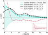 |
Fig. 17. Radial convergence profiles of the quasar sample in the redshift range 1.2 ≤ z ≤ 2.8, divided into redshift intervals and considering quasar pairs. Inset Panel: Quasar pairs in the redshift range z ∈ [2.2, 2.8] with their corresponding cosmic variance, showing a negligible signal-to-noise ratio. |
Figure 18 shows the radial convergence profiles for isolated quasars and quasar pairs in this redshift range. For isolated quasars, we further divided the sample into two new subsets: high-luminosity and low-luminosity quasars, according to the median luminosity of the total sample. It is clear that even with this sub-sampling, there is no difference in signal for the isolated quasars. However, as in the case of the cross-correlation function, quasar pairs exhibit a signal significantly higher than that of the isolated quasar sample. Furthermore, dividing the pairs into high- and low-luminosity pairs based on the median of L1 + L2, we find that the most luminous quasars contribute the strongest signal to the total sample. This significance is confirmed by considering random positions in the CMB map to estimate the cosmic variance of the sample of pairs, showing a high noise-signal relation.
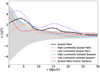 |
Fig. 18. Radial convergence profiles for quasar pairs in the redshift range 1.2 ≤ z ≤ 2.2, categorized by luminosity levels (dotted lines for high- and low- luminosity pairs). For comparison, the profiles of isolated quasars are shown with dashed lines. The results indicate that the amplitude of the radial convergence for quasar pairs consistently exceeds that of isolated quasars. Moreover, high-luminosity quasar pairs contribute significantly to a signal that surpasses the expected cosmic variance. |
8. Summary and discussion
In this study, we constructed a subsample from the SDSS DR16 quasar catalog, focusing on the redshift range (z ∈ [1.2, 2.8]), where the sample exhibits good completeness. We conducted a comprehensive analysis of this subsample, with particular emphasis on the detection of quasar pairs. To achieve this, we first calculated the projected distance in Mpc between the two members of each quasar pair.
We performed an extensive exploratory analysis of the luminosity distribution of the quasar pairs, examining how they differ from both control and simulated pairs. Moreover, we computed the cross-correlation function between quasar pairs and the overall quasar population, revealing a distinctly amplified signal above the background of isolated quasars. We investigated how this correlation is influenced by various scenarios, including partitioning the redshift interval into two segments, separating the data according to the radio luminosity ratio L1/L2, and applying a cutoff in log10(L1 + L2)/L⊙. The main amplitude of the cross-correlation signal remains consistent under these conditions. We also addressed the observational capabilities for detecting quasar pairs using the SDSS camera, discussed the possibility of contamination of the quasar pair sample by foreground galaxies, and contrasted the numerical comoving density of the quasar pairs with that of the quasar subsample.
We demonstrate that the CMB convergence signal remains within the bounds defined by cosmic variance estimates for the redshift interval z ∈ [1.2, 2.8]. When we refine our focus to a narrower redshift range, z ∈ [1.2, 2.2], the CMB convergence signal associated with quasar pairs exhibits a heightened amplitude, surpassing not only that of the total quasar pair sample, but also the estimated cosmic variance, as illustrated in Fig. 17.Furthermore, our analysis confirms that the amplitude of the cross-correlation between quasar pairs and individual quasars consistently exceeds that of the quasar autocorrelation within the same redshift range (see Fig. 13). By integrating the cross-correlation function with the CMB convergence signal, we achieved a substantially enhanced detection rate of quasar pairs at lower redshifts, culminating in a total of Np = 2126.
We further validated our detection through an additional observational test, focusing on the amplitude of the CMB lensing signal associated with quasar pairs distinguished by high and low luminosities, using the mean luminosity as the cutoff between these two groups. Our analysis reveals that the most luminous pairs of quasars are the dominant contributors to the overall signal for the sample, as illustrated in Fig. 18.
This work provides a valuable foundation for further investigation into the characterization of the large-scale structure of the Universe by integrating the cross-correlation function obtained from quasar catalogs with an in-depth analysis of the CMB convergence lensing signal.
Data Availability
The data that support the findings of this study will be available on reasonable request.
The SDSS DR16Q quasar sample exhibits characteristic statistical redshift uncertainties on the order of |Δz|≃0.001 Lyke et al. (2020).
A similar analysis was carried out on 500 random sets of synthetic pairs generated from the isolated set, showing no significant deviations.
While our focus is on the redshift interval z ∈ [2.2, 2.8], it is noteworthy that a similar analysis has been conducted across other redshift bins, yielding comparable results.
The bootstrap algorithm offered several advantages in our statistical analysis. Specifically, it provided a more robust estimate of uncertainties by allowing replacement resampling, which better captured the underlying distribution of the data. It was particularly beneficial when the quasar pair dataset size was small compared to the larger quasar sample, ensuring that we accounted for variability and improved our confidence in the derived results.
We investigated various values of the resampling number Nrs and found that the results remain largely invariant, showing no significant variation across the different configurations tested.
To better understand the significance of our earlier results, we consider the formulation of the signal-to-noise ratio in the context of cross-correlation:  . This expression highlights that a nonzero pair detection is fundamentally encoded in the amplitude of the cross-correlation function, ξpq(s), when juxtaposed against the background of the quasars Menard & Bartelmann (2002). Here, the interaction between the number of quasars Nq and the number of potential counterparts Np amplifies the measurement sensitivity, allowing genuine correlations to be discerned amidst the noise inherent in the quasar distribution.
For the other redshift partition (2.5 ≤ z ≤ 2.8), we encounter no significant variance issues, allowing us to proceed with a standard linear regression analysis. Indeed, when we conduct a comprehensive nonlinear fit for the initial eight bins, we obtain a correlation length given by s0 = (16.00 ± 1.94) Mpc h−1 and the exponent is γ = (1.65 ± 0.16).
Acknowledgments
We acknowledge the use of the SDSS DR16 catalog https://www.sdss4.org/dr16/algorithms/qso_catalog, Lyke et al. (2020). We used several packages such as Astropy Astropy Collaboration (2013), Corrfunc Sinha (2013), Numpy Oliphant (2006), Matplotlib Hunter (2007), Scipy Virtanen et al. (2020), Healpy Zonca et al. (2019), HEALPix Górski et al. (2005), Pandas McKinney (2010). The authors thank CNPq, FAPES, and Fundação Araucária for financial support. The authors would like to express their gratitude for the valuable comments provided by the referee, which significantly contributed to enhancing the quality and clarity of the paper.
References
- Alberts, S., & Noble, A. 2022, Universe, 8, 11 [Google Scholar]
- Astropy Collaboration (Robitaille, T. P., et al.) 2013, A&A, 558, A33 [NASA ADS] [CrossRef] [EDP Sciences] [Google Scholar]
- Bennert, V. N., Auger, M. W., Treu, T., et al. 2011, ApJ, 742, 107 [Google Scholar]
- Chen, Y. C., Liu, X., Foord, A., et al. 2023, Nature, 616, 45 [NASA ADS] [CrossRef] [Google Scholar]
- Croom, S. M., Boyle, B. J., Shanks, T., et al. 2005, MNRAS, 356, 415 [NASA ADS] [CrossRef] [Google Scholar]
- Eftekharzadeh, S., Myers, A. D., White, M., et al. 2015, MNRAS, 453, 2779 [Google Scholar]
- Eltvedt, A. M., Shanks, T., Metcalfe, N., et al. 2024, MNRAS, 535, 2105 [Google Scholar]
- Fanidakis, N., Macció, A. V., Baugh, C. M., et al. 2013, MNRAS, 436, 315 [NASA ADS] [CrossRef] [Google Scholar]
- Geach, J. E., Peacock, J. A., Myers, A. D., et al. 2019, ApJ, 874, 85 [Google Scholar]
- Górski, K. M., Hivon, E., Banday, A. J., et al. 2005, ApJ, 622, 759 [Google Scholar]
- Guo, H., Liu, X., Shen, Y., et al. 2019, MNRAS, 482, 3288 [Google Scholar]
- Haehnelt, M. G., & Kauffmann, G. 2000, MNRAS, 318, L35 [NASA ADS] [CrossRef] [Google Scholar]
- Harrison, C. M., Costa, T., Tadhunter, C. N., et al. 2018, Nat. Astron., 2, 198 [Google Scholar]
- Hunter, J. D. 2007, Comput. Sci. Eng., 9, 90 [NASA ADS] [CrossRef] [Google Scholar]
- Ishikawa, Y., Zakamska, N. L., Shen, Y., et al. 2025, ApJ, 982, 22 [Google Scholar]
- Jing, L., et al. 2025, arXiv e-prints [arXiv:2505.03103] [Google Scholar]
- Kauffmann, G., & Heckman, T. M. 2009, Nature, 460, 199 [Google Scholar]
- Kormendy, J., & Ho, L. C. 2013, ARA&A, 51, 511 [Google Scholar]
- Landy, S. D., & Szalay, A. S. 1993, ApJ, 412, 64 [Google Scholar]
- Laurent, P., Eftekharzadeh, S., Le Goff, J.-M., et al. 2017, JCAP, 07, 017 [Google Scholar]
- Lyke, B. W., Higley, A. N., McLane, J. N., et al. 2020, ApJS, 250, 24 [Google Scholar]
- McKinney, W. 2010, in Proceedings of the 9th Python in Science Conference, eds. S. van der Walt, & J. Millman, 56 [Google Scholar]
- Menard, B., & Bartelmann, M. 2002, A&A, 386, 784 [NASA ADS] [CrossRef] [EDP Sciences] [Google Scholar]
- Merloni, A., & Heinz, S. 2007, MNRAS, 381, 589 [Google Scholar]
- Mohammad, F. G., & Percival, W. J. 2022, MNRAS, 514, 1289 [NASA ADS] [CrossRef] [Google Scholar]
- Muldrew, S. I., Hatch, N. A., & Cooke, E. A. 2015, MNRAS, 452, 3 [Google Scholar]
- Norberg, P., Baugh, C. M., Gaztañaga, E., & Croton, D. J. 2009, MNRAS, 396, 19 [Google Scholar]
- Oliphant, T. E. A. 2006, A guide to NumPy (USA: Trelgol Publishing), 1 [Google Scholar]
- Pâris, I., Petitjean, P., Aubourg, E., et al. 2012, A&A, 548, A66 [NASA ADS] [CrossRef] [EDP Sciences] [Google Scholar]
- Peng, C. Y., Impey, C. D., Rix, H.-W., et al. 2006, ApJ, 649, 616 [Google Scholar]
- Petter, G. C., Hickox, R. C., Alexander, D. M., et al. 2022, ApJ, 927, 16 [Google Scholar]
- Planck Collaboration VIII. 2020, A&A, 641, A8 [NASA ADS] [CrossRef] [EDP Sciences] [Google Scholar]
- Porciani, C., Magliocchetti, M., & Norberg, P. 2004, MNRAS, 355, 1010 [NASA ADS] [CrossRef] [Google Scholar]
- Richards, G. T., Strauss, M. A., Fan, X., et al. 2006, AJ, 131, 276 [Google Scholar]
- Ross, N. P., McGreer, I. D., White, M., et al. 2013, ApJ, 773, 14 [NASA ADS] [CrossRef] [Google Scholar]
- Schneider, D. P., Fan, X., Hall, P. B., et al. 2003, AJ, 126, 2579 [Google Scholar]
- Shen, Y., Strauss, M. A., Ross, N. P., et al. 2009, ApJ, 697, 1656 [Google Scholar]
- Silk, J., & Rees, J. M. 1998, A&A, 331, L1-14 [Google Scholar]
- Sinha, M. 2013, Corrfunc Documentation V2.5.1: https://github.com/manodeep/Corrfunc [Google Scholar]
- Sinha, M., & Garrison, L. H. 2020, MNRAS, 491, 3022 [Google Scholar]
- Song, H., Park, C., Lietzen, H., et al. 2016, ApJ, 827, 104 [CrossRef] [Google Scholar]
- Toscano, F., Luparello, H., Gonzalez, E. J., et al. 2023, MNRAS, 526, 5393 [Google Scholar]
- Virtanen, P., Gommers, R., Oliphant, T. E., et al. 2020, Nat. Methods, 17, 261 [Google Scholar]
- White, M., Myers, A. D., Ross, N. P., et al. 2012, MNRAS, 424, 933 [NASA ADS] [CrossRef] [Google Scholar]
- Wu, Q., & Shen, Y. 2022, ApJS, 263, 42 [NASA ADS] [CrossRef] [Google Scholar]
- Zehavi, I., Zheng, Z., Weinberg, D. H., et al. 2011, ApJ, 736, 59 [NASA ADS] [CrossRef] [Google Scholar]
- Zonca, A., Singer, L., Lenz, D., et al. 2019, J. Open Source Software, 4, 1298 [Google Scholar]
All Figures
|
Fig. 1. Top panel: Projection of the 3D map representation of quasars from the SDSS DR16Q catalog; the color bar indicates the redshifts of each quasar. Bottom panel: Redshift distribution of the quasars, normalized by the total number of objects in the sample. The median of this distribution is marked by a distinct point for clarity. The subsample within the redshift range z ∈ [1.2, 2.8] is highlighted by vertical lines. |
| In the text | |
|
Fig. 2. Absolute magnitude across the redshift range. The magnitude bands are defined according to the relationship |M|I(z) = |M|0 + 1.8(z − 0.8). |
| In the text | |
|
Fig. 3. Top panel: Mask used to generate a random map at a resolution of Nside = 32, incorporating a smoothing factor of θs = 4°. Bottom panel: The yellow region represents the dataset points, while the green region highlights the random points generated using the probability density function alongside the smoothing mask. The overlap between both sets indicates a strong level of concordance. |
| In the text | |
|
Fig. 4. Top panel: Two-point correlation function obtained using the LS estimator for the total sample, z ∈ [1.2, 2.8]. Red point represents the correlation function with its error bars. Bottom panel: The dashed red curve indicates the best linear fit in logarithm scale. In the linear regime, the correlation function can be parametrized as ξ(s) = (s/s0)−γ with γ = 1.21 ± 0.03 and s0 = 12.25 ± 1.30. |
| In the text | |
|
Fig. 5. Top panel: Distribution of quasar pairs across the complete redshift window of the SDSS DR16 quasar catalog. The highest concentration of pairs is found within the redshift range z ∈ [1.2, 2.8], totaling 2777 pairs. The catalog contains a total of 4011 pairs. Bottom panel: Distribution of quasar pairs detected within a cylindrical volume characterized by a projected radius of dp ≤ 2 Mpc and a length of |ΔV| = 900 km/s. Black vertical lines denote |
| In the text | |
|
Fig. 6. Scatter plot of the 2777 quasar pairs that satisfy the criterion |ΔV|≤900 km/s. The color bar, normalized across the dataset, represents the redshift variation, Δz, between quasar pairs, effectively conveying this continuous variable through a color scale. |
| In the text | |
|
Fig. 7. Histogram of the quasar luminosity distribution after applying K-corrections. The horizontal axis is displayed on a logarithmic scale. |
| In the text | |
|
Fig. 8. Distribution of luminosity ratios for true quasar pairs and control pairs. The true quasar pairs are indicated in blue, while the control pairs are shown in gray. |
| In the text | |
|
Fig. 9. Distribution of the logarithm of the sum of luminosities for true quasar pairs and control pairs. True quasar pairs are shown in blue, while control pairs are shown in gray. |
| In the text | |
|
Fig. 10. Distribution of luminosity ratios for true quasar pairs and simulated pairs is illustrated. True quasar pairs are shown in blue, while simulated pairs are shown in gray. |
| In the text | |
|
Fig. 11. Top panel: Color-color map for the entire subsample of quasars. Bottom panel: Color-color map for the detected quasar pairs. Here, log(N) represents the logarithm of the number of quasar pairs within each region of the color-color map. Note that in some cases, the maximum or minimum values may lie outside the displayed data range. |
| In the text | |
|
Fig. 12. Different color-color maps for the quasar pairs. |
| In the text | |
|
Fig. 13. Top panel: Comparison of the two-point cross-correlation function, derived using the LS estimator between quasar pairs and individual quasars within the 1.2 ≤ z ≤ 2.8 redshift window. The cross-correlation is shown alongside autocorrelation for the full sample in that interval and for isolated quasars. Bottom panel: Linear regressions for the three cases are depicted on a logarithmic scale to visualize their slopes. The estimates of (γ, s0) remain consistent across all three cases. |
| In the text | |
|
Fig. 14. Top panel: Two-point cross-correlation function obtained using the LS estimator between quasar pairs and individual quasars at intermediate redshift. The 2PCF for the entire sample, computed using a bootstrap method for resampling, is also included. Bottom panel: The same 2PCF functions are shown on logarithmic scales. |
| In the text | |
|
Fig. 15. Top panel: Two-point correlation function derived using the LS estimator for the cross-correlation between quasar pairs and individual quasars within the redshift interval 2.2 ≤ z ≤ 2.5. The 2PCF for the entire subsample is included, computed using the resampling bootstrap method, as well as the 2PCF for isolated quasars not belonging to any pair. Bottom panel: The same 2PCFs are presented on a logarithmic scale. |
| In the text | |
|
Fig. 16. Top panel: Comparison of two-point cross-correlation functions obtained using the LS estimator between quasar pairs and individual quasars in the 2.2 ≤ z ≤ 2.8 redshift window, shown with different partition criteria. Bottom panel: The same two-point cross-correlation functions are displayed on logarithmic scales to visualize their slopes. |
| In the text | |
|
Fig. 17. Radial convergence profiles of the quasar sample in the redshift range 1.2 ≤ z ≤ 2.8, divided into redshift intervals and considering quasar pairs. Inset Panel: Quasar pairs in the redshift range z ∈ [2.2, 2.8] with their corresponding cosmic variance, showing a negligible signal-to-noise ratio. |
| In the text | |
|
Fig. 18. Radial convergence profiles for quasar pairs in the redshift range 1.2 ≤ z ≤ 2.2, categorized by luminosity levels (dotted lines for high- and low- luminosity pairs). For comparison, the profiles of isolated quasars are shown with dashed lines. The results indicate that the amplitude of the radial convergence for quasar pairs consistently exceeds that of isolated quasars. Moreover, high-luminosity quasar pairs contribute significantly to a signal that surpasses the expected cosmic variance. |
| In the text | |
Current usage metrics show cumulative count of Article Views (full-text article views including HTML views, PDF and ePub downloads, according to the available data) and Abstracts Views on Vision4Press platform.
Data correspond to usage on the plateform after 2015. The current usage metrics is available 48-96 hours after online publication and is updated daily on week days.
Initial download of the metrics may take a while.