| Issue |
A&A
Volume 700, August 2025
|
|
|---|---|---|
| Article Number | A56 | |
| Number of page(s) | 14 | |
| Section | Extragalactic astronomy | |
| DOI | https://doi.org/10.1051/0004-6361/202555273 | |
| Published online | 05 August 2025 | |
Characterizing the outer disk of extended-UV galaxies in the optical domain with deep surveys
1
Aix Marseille Univ, CNRS, CNES, LAM, Marseille, France
2
Instituto de Astrofísica de Canarias, Vía Láctea S/N, E-38205 La Laguna, Spain
3
Departamento de Astrofísica, Universidad de La Laguna, E-38206 La Laguna, Spain
4
National Centre for Nuclear Research, Pasteura 7, 02-093 Warsaw, Poland
5
Instituto de Astrofísica, Pontificia Universidad Católica de Chile, Vicuña Mackenna 4860, 7820436 Macul, Santiago, Chile
⋆ Corresponding author: This email address is being protected from spambots. You need JavaScript enabled to view it.
Received:
23
April
2025
Accepted:
11
June
2025
Abstract
Aims. Extended-UV (XUV) galaxies are galaxies that present an extended outer ultraviolet disk. Although some giant low surface brightness (GLSB) galaxies are also XUV, their relation has been seldom studied. This work aims to determine whether a sample of nine XUV galaxies can be classified as GLSB galaxies, by analyzing their photometric properties in deep optical images.
Methods. The method presented here used optical data from the Dark Energy Survey to construct surface brightness profiles for each galaxy. We defined a characteristic UV radius to examine the XUV disks. We fitted the surface brightness profiles using simple exponential functions, and compared the extracted parameters with the literature to identify possible GLSB galaxies. We also examined other diagnostics, including color profiles.
Results. The analysis of the optical surface brightness profiles of XUV galaxies reveals that they can be classified into three different families. One third meet the GLSB criteria in terms of diffuseness, another third are regular, and the remaining have a stronger decline in the outer disk than in the inner disk, which is opposite to the characteristics of GLSB galaxies. The color profile allowed us to distinguish one galaxy, NGC1140, and speculate that it is the result of a rare dwarf-dwarf merger.
Key words: galaxies: evolution / galaxies: general / galaxies: structure
© The Authors 2025
 Open Access article, published by EDP Sciences, under the terms of the Creative Commons Attribution License (https://creativecommons.org/licenses/by/4.0), which permits unrestricted use, distribution, and reproduction in any medium, provided the original work is properly cited.
This article is published in open access under the Subscribe to Open model. This email address is being protected from spambots. You need JavaScript enabled to view it. to support open access publication.
1. Introduction
Low surface brightness (LSB) galaxies are a major class of galaxies, as demonstrated by O’Neil & Bothun (2000) and Minchin et al. (2004), who showed that they could account for about half of the total galaxy population. Their large number was confirmed in later studies. For example, Martin et al. (2019) simulations suggest that LSBs are estimated to account for 85% of the local number density for stellar mass above a threshold of M⋆ > 107 M⊙. The importance of LSB galaxies has increased with the discovery of their number, but also due to the possible new insights into extragalactic physics that they offer. For instance, researchers soon realized that various types of LSB galaxies may be dark-matter-dominated (Zwaan et al. 1995; McGaugh & de Blok 1998) or enable constraints on the nature of dark matter (Kravtsov 2024; Lelli et al. 2010), and they offer an additional constraint for cosmological models in general (Boquien et al. 2019; Haslbauer et al. 2019).
Low surface brightness galaxies were first defined as galaxies with a disk central surface brightness in the B-band significantly lower than 21.65 mag.arcsec−2, the value found by Freeman (1970) for a small sample of regular nearby galaxies. However, later studies (Bothun et al. 1997; McGaugh et al. 1995) demonstrated that this value was biased by selection effects, as predicted by Disney (1976). Several definitions of LSBs can be found in the literature (e.g., Bothun et al. 1997; McGaugh et al. 1995; Monnier Ragaigne et al. 2003) and they are often described as galaxies with a surface brightness lower than the sky background (around 22.5–23 mag.arcsec−2), with variations on the adopted limit and the band.
After early discoveries made with photographic plates, progress in observational methods, the use of couple-charge devices (CCDs), and large sky surveys (e.g., Sloan Digital Sky Survey, Abazajian et al. 2009) have increased the number of known LSB galaxies, but also of dedicated studies. This is likely to continue in the coming years with the new deep surveys such as the Dark Energy Survey (DES, Abbott et al. 2021), Euclid (Euclid Collaboration: Mellier et al. 2025), and the Vera C. Rubin Observatory Legacy Survey of Space and Time (LSST, Ivezić et al. 2019).
As was quickly realized, a rich variety exists among LSB galaxies. Sprayberry et al. (1995) proposed to distinguish giant LSB (GLSB) galaxies based on the measurement of the central surface brightness and the scale length of the disk component. They introduced the concept of diffuseness to delimit the GLSB galaxies from more regular LSB galaxies. The most extreme GLSB galaxy (which we will use as a reference in our study) is Malin 1, which was unexpectedly found by Bothun et al. (1987) and is still the largest known spiral, star-forming galaxy. The discovery of giant star-forming disks called galaxy formation models into question and led to further studies of these galaxies. After Malin 1, other GLSB galaxies were discovered (see the compilation in Sprayberry et al. 1995), and new GLSB galaxies have been found in more recent years with the help of new imaging surveys (e.g., Hagen et al. 2016; Saburova et al. 2021). These galaxies are characterized by their large-scale length, extremely low central surface brightness, but also, usually, by an important gas mass, with HI mass above 1010 M⊙. Their formation mechanism remains an open question, with multiple hypotheses proposed to explain their origin (e.g., Boissier et al. 2016; Hagen et al. 2016; Saburova et al. 2018).
Another class of LSB galaxies that has been widely discussed in recent years (van Dokkum et al. 2015; Koda et al. 2015; Yagi et al. 2016; Mihos et al. 2015; Junais et al. 2021) are ultra-diffuse galaxies (UDGs). This is a very faint population, defined by their large sizes (reff > 1.5 kpc) and very low surface brightness (μ0,g > 24 mag arcsec−2), but they are not within the scope of this paper.
While all these definitions were proposed on the basis of the diagnostic made in the optical, after the launch of Galaxy Evolution Explorer (GALEX) (Morrissey et al. 2005) in 2003, it was quickly discovered that 30% of regular galaxies present an extended LSB component in the UV and were called extended UV (XUV) galaxies (Gil de Paz et al. 2005; Thilker et al. 2007). These galaxies are characterized by an UV-emitting disk that extends well beyond the optical radius R25 defined as the radius where the surface brightness reaches 25 mag arcsec−2 in the B band. This finding revealed ongoing star formation in regions where little or no star formation was previously expected. Thilker et al. (2007) defined two different types of XUV galaxies. Type 1 XUV galaxies are characterized by structured and bright UV emission located beyond the expected threshold for star formation. Type 2 XUV galaxies have disks that exhibit blue colors (FUV–NIR) across a large, outer region of the disk with low optical surface brightness.
Studies of the UV properties of GLSB galaxies suggested that some GLSB galaxies are, in fact, also XUV galaxies (Boissier et al. 2008; Hagen et al. 2016). This finding leads to a questioning of the potential link between these two types of galaxies with faint extended disks. Although the UV emission at LSB in GLSB galaxies suggested this connection, the definition of XUV galaxies was made by comparing deep UV to less deep optical images (e.g., SDSS). The opposite question of whether XUV galaxies are systematically GLSB galaxies when characterized in the optical, is still open. In this work, we propose to tackle this issue and characterize classical XUV galaxies from Thilker et al. (2007) in the optical, for which deeper optical images are now available with DES.
In Section 2 we present the sample selection, the method, and the image processing of the DES data we used to compute the surface brightness profiles. Section 3 presents the surface brightness profiles obtained with DES and GALEX data, and we compare our method with the literature. We also propose to compute a physically based UV radius and a diagnostic in order to characterize the UV disk of the XUV galaxies. To extend the analysis, we checked the color profiles and spectral energy distribution (SED) fitting results of the sample. In Section 4, we discuss a particular galaxy that distinguishes itself from the rest of the sample, and the possible future of this field with new instruments, before concluding in Section 5.
2. Sample and data
2.1. Sample selection
In order to characterize in the optical the regions detected in UV in XUV galaxies, we cross-correlated the Thilker et al. (2007) catalog of 54 classical XUV galaxies with the publicly available deep optical images from DES (Abbott et al. 2021). In this paper, we analyze the nine XUV galaxies from Thilker et al. (2007) with available deep DES optical data (g, r, i, z, Y) from DR2 and GALEX (FUV and NUV) images. The main properties of the sample are reported in Table 1. This small sample includes both type 1 and type 2 XUV galaxies and broadly covers the RC3 T-type of the parent sample of Thilker et al. (2007). The morphological type is given in Table 1. Some GLSB galaxies have been found in previously misclassified, early-type galaxies (Hagen et al. 2016). We take all the XUV galaxies from Thilker et al. (2007) independently of their morphological type.
Properties of the sample.
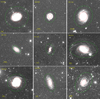 |
Fig. 1. DES images of the sample in g band. The ellipses show the adopted position angle and ellipticity at the R25 (RUV) radius in red (green). |
2.2. Image processing
We produced cutouts of DES and GALEX images with a width of 800 arcsec (except for NGC300 for which we used 4000 arcsec by coadding four tiles of DES) in order to ensure that we probed the extended disk and kept the background sky in the vicinity of the galaxy. For the GALEX images, we took the archival images available in the GR6/7 Data Release (https://galex.stsci.edu/gr6/), and we stacked the multiple exposures within the field of the cutout using the reproject package (Robitaille et al. 2023). We projected the GALEX images with a pixel scale of 1.5 arcsec pixels to the DES pixel scale of 0.263 arcsec again using the reproject tool.
Some galaxies (in particular NGC 1042) have bright neighbors. This causes fluctuations and flux contamination in the images and increases the uncertainties in the faint and extended parts. The first step to limit this effect is to mask all sources in the g+r images, including the galaxy itself, using segmentation from photutils (Bradley et al. 2024). We then fit the masked image with a second order polynomial, as in Merritt et al. (2016). This sky gradient is subtracted from the images.
In order to estimate the sky characteristics, we created 24 boxes (of varying size from 70 arcsec to 437 arcsec depending on the size of the cutout) around each galaxy. In each of them, we computed the mean (μ) in each box in the masked images (using the g+r mask created before). The boxes with a mean greater than three sigma from the average of the means (⟨μ⟩) were excluded to avoid boxes with badly masked bright stars or artifacts.
The masked pixels were replaced by the mean sky value (⟨μ⟩) calculated above. We then applied a 13 × 13 pixels binning. This value was chosen by comparing the binning applied by Pohlen & Trujillo (2006) to NGC 1042 with the SDSS data deferred to the DES pixel size. Field stars that overlapped with the galaxy were replaced by the mean value measured in a circular annulus around them using the function SkyCircularAnnulus of photutils.
Some faint artifacts or stars made visible by the binning were masked again in the binned image that we ultimately used to compute the sky properties in the same boxes as above: the mean of the number of pixels (NPix), mean of the means (⟨μ⟩), the mean of the standard deviation in each box (ep), and the standard deviation of the means (es). These constants allowed us to compute the surface brightness uncertainties (used in Section 3.1) following Equation (1) from Gil de Paz & Madore (2005):
 (1)
(1)
with

Ndata represents the number of data points. This method of computing errors is as conservative as possible, and takes into account both the normal distribution on the pixel scale measured by ep and the eventual variations on large scales, measured by es, while errors in the literature often only refer to the normal distribution in carefully chosen regions.
3. Analysis and results
3.1. Surface brightness profiles
In order to obtain surface brightness profiles at the same location in all the bands for each galaxy, the position angle (PA) and ellipticity are fixed following the idea of Pohlen & Trujillo (2006) to determinate these parameters in a deep image, adequate for the outer parts of the disks. It has the following advantages: in the outer regions with a low signal, it avoids the PA changing arbitrarily, and it is a method consistent with many surface brightness profiles from the literature (Trujillo et al. 2021; Merritt et al. 2016; Pohlen & Trujillo 2006). We also performed an experiment in which we let the PA and ellipticity vary freely for NGC1512, whose geometry varies the most with radius. The results of this test were consistent with our method and the conclusions of this work remained unchanged.
We first generated a set of ellipses in the g band with EllipseGeometry and Ellipse from the photutils package with the center fixed, and the PA and the ellipticity (e) set as free parameters. For these free parameters, a guess was provided, but weverified that it has no impact on the final results. We then selected the ellipse that reached a surface brightness one sigma above the sky mean, following Pohlen & Trujillo (2006). In this way, we kept the ellipses as close as possible to the shape of the external disk of the galaxy.
The resulting PA and e are given in Table 2. Then a new set of ellipses with a spacing of 4 arcsec was defined with these parameters fixed. We used this set of ellipses to measure the surface brightness profiles in each band with the function fit_isophote from Photutils, as shown in Fig. 2. The profiles were cut whenever the measured profile reached the sky value or the errors were too large (above one magnitude). The complete profiles with their uncertainties are provided in an electronic form at CDS. We compared the GALEX profiles obtained with other profiles available in the literature. We found that our profiles are similar to those published by Bouquin et al. (2018) but generally extend to larger radii than those analyzed in Gil de Paz et al. (2007).
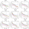 |
Fig. 2. Observed surface brightness profiles for each band of the sample as a function of the semimajor axis of the ellipses. The dashed gray line is the R25 and the dashed black line is the RUV defined in Section 3.3.1. For clarity, an offset have been applied on the profiles of +n magnitudes/arcsec2 with a dependence on the bands indicated in the bottom right panel. The dotted blue line represents 25 mag.arcsec−2 in the B band adapted to the g band using Fukugita et al. (1995). |
Properties of the sample computed for this work.
3.2. Robustness of the method
Among our nine galaxies, NGC 1042 was observed in the g band with the Large Binocular Telescope (LBT, Trujillo et al. 2021) and Dragonfly (Merritt et al. 2016) to study its outer parts and stellar halo. This gave us the opportunity to perform several tests to ensure that the DES images are deep enough (and our method robust enough) to study the region of the galaxy responsible for the extended UV emission.
First, we computed the surface brightness with the LBT data using the method described in Sects. 2.2 and 3.1. We obtained a very similar profile to the one from Trujillo et al. (2021), calculated with the same data but with a different approach (see the top panel of Fig. 3). Our error bars are larger than theirs, which can be attributed to the more conservative approach adopted in calculating uncertainties that include a large-scale-fluctuation component (see Equation (1)).
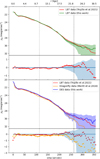 |
Fig. 3. Surface brightness profile in g band for NGC 1042 as a function of the semimajor axis (sma) of ellipses. Top: Comparison of the method with the profile from Trujillo et al. (2021) with LBT data (in red) and our method applied to the same data (in green), and the difference between them under the main panel. Bottom: Comparison of the data with the profile from Trujillo et al. (2021) with LBT data (in red), the profile from Merritt et al. (2016) with Dragonfly data, and our method applied to DES data (in blue). The differences between the other profiles and ours are shown under the main panel. The dashed gray line is the R25 of the galaxy when the dashed black line is the RUV. The shaded area shows the uncertainties for LBT data with the method used here in the top panel and DES data with the method used here in the bottom panel. |
Second, we compared the surface brightness profile obtained with the DES data and our method with the Trujillo et al. (2021) LBT surface brightness profile (bottom panel of Fig. 3). This step allowed us to verify that our method allows us to measure a surface brightness profile up to the largest radii measured by Trujillo et al. (2021), here again with large uncertainties at the largest radii. Small differences between the data are visible just before the UV radius (defined in Section 3.3.1), and do not affect our results. We show one sigma upper limits in the profiles whenever the measured flux minus the uncertainty is lower than zero. The uncertainties are slightly larger than those obtained with the LBT data, which is directly related to the relative noise of the LBT and DES images. Importantly, the uncertainties remain small in the “XUV region” that we want to analyze, and are under one mag.arcsec−2 at its outer edge (see Section 3.3.2 for a definition of our maximum radius of analysis).
We also compared our profiles with the one obtained by Merritt et al. (2016) with Dragonfly for this galaxy (lower panel of the Fig. 3). We note that the Dragonfly profile drops to a surface brightness lower than the DES or LBT profiles at the largest radii, but our conservative uncertainties encompass it.
As a further test, we applied a coarser binning in DES images of 65 × 65 pixels to obtain a similar pixel scale as the Dragonfly value of 2.85 arcsec/pixel with the binning they used, running a first set of ellipses on g + r images (instead of g in our case) and using those ellipses to compute the g band profile. The profile obtained in this procedure is consistent with the one obtained above, without improving it. As shown in Fig. 2, some of the profiles flatten in the very outer parts, particularly for NGC 991, NGC 1042 (see also Fig. 3), NGC 1140, and NGC 2090. This flattening begins when the flux is close to the sky value and the uncertainties are high.
We thus consider that our data and methods are robust in comparison to other data sources and methodology to produce a surface brightness profile in the UV emitting regions, and we adopt it for the rest of this study. All data in the following sections have been corrected for inclination by multiplying the fluxes by

The data hereafter are also corrected for Galactic extinction, Aλ. For each band, the extinction law  is calculated using Cardelli et al. (1989). Then we subtracted from the profiles the attenuation

the reddening E(B − V) is given in Table 1, and Rv is set to a value of 3.1.
According to our profiles, the R25 seems to be further out than the one adopted in Thilker et al. (2007), as can be seen from Figure 2. In order to check how much our results depend on the determination of R25, we calculated our own value based on the g-band profile, converted to B band using Fukugita et al. (1995). We found small changes (between six and thirteen arcsec) in most cases, except for two galaxies (117 arcsec for NGC 0300, 20% smaller, and 24 arcsec for NGC 0991, 50% larger). We verified that our results and figures are qualitatively unchanged if this value is adopted. For consistency with previous works, we show our results adopting the value of R25 from the literature for the rest of the analysis.
3.3. Characterization of the XUV galaxies
3.3.1. Determination of RUV
The size of galaxies in the UV is frequently defined as the last galaxy radius with useful UV data (Gil de Paz et al. 2007; Boissier et al. 2008). This definition is not satisfactory, especially in light of our goal to characterize the UV extended region, as it depends on the data. We thus propose to adopt a definition that is consistent across all galaxies and physically motivated, by basing it on the star formation rate surface density.
To do so, we converted the inclination and Galactic extinction corrected surface brightness profile in the FUV band of GALEX into a flux, Fν, in ergs s−1 Hz−1 cm−2, and then into a star formation rate surface density following Equation (2):
 (2)
(2)
The C constant (0.97 × 10⁻²⁸) represents the Ultraviolet-star formation rate (UV-SFR) calibration, for which we adopt the value of Boissier (2013) using the IMF of Kroupa (2001). The results are shown in Fig. 4. Then, for RUV, we adopted the radius where the SFR surface density is equal to ΣSFR = 10−2 M⊙ Gyr−1 pc−1. This value is well reached in all the GALEX profiles and it corresponds to what is typically found in the very outer regions of nearby galaxies studied in Bigiel et al. (2008), and to the value far out in the disk of Malin 1 (Junais et al. 2024). This radius is thus well consistent with the largest star-forming regions observed in galaxies in general. The RUV obtained for each galaxy in our sample is given in Table 2. Fig. 4 shows that RUV in our XUV galaxies is, of course, much larger than R25, ranging from about 2 to 3.5 R25.
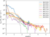 |
Fig. 4. Star formation rate surface density (ΣSFR) as a function of the semimajor axis normalized to the R25. The dashed gray line is the value that corresponds to the RUV. |
3.3.2. Optical characterization of the extended UV region
In this section, we aim to characterize in the g band the regions where UV emission is found at a large radius in XUV galaxies. Large diffuse disks have been classically studied in the optical. Sprayberry et al. (1995) proposed a diagnostic plot showing the central surface brightness versus the scale length of the disk component of such galaxies.
In order to add the XUV selected disks in this (optical) diagnostic plot, we applied the following procedure. The profiles are fitted with simple exponential functions in the g band in the inner region and outer regions of our galaxies.
The inner region is defined as the area within the radius R25 of the galaxy, while the outer region corresponds to radii ranging from R25 to RUV, the latest being defined in Sect. 3.3.1. For each galaxy, we applied an exponential fit to the radial profile in each region and show the results in Fig. 5. For each region, we thus obtained the central surface brightness and the scale length (μ0, g and Rs) that are given in Table 2.
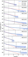 |
Fig. 5. Surface brightness profiles in g band of the sample as a function of the radius normalized by R25. The dashed gray line is the R25 and the black one is the RUV. The dotted green line is the fit in the outer region and the dotted red line is the fit in the inner region. |
This procedure does not necessarily provide a perfect fit (see Fig. 5), but is extremely simple and easy to reproduce. A bulge-disk decomposition could be more effective. We tried this approach by fitting two exponential components and De Vaucouleur profiles. We obtained very similar scale lengths and central surface brightnesses of the disk component for six galaxies. However, the remaining three galaxies (NGC6902, NGC2090, and NGC1140) were dominated by an early-type profile at all radii inside R25, which shows that this approach is difficult to apply systematically. We also tried to determine these parameters after excluding the most inner points that may be affected by a bulge, and found very similar values.
In order to compare to Sprayberry et al. (1995), the profiles were converted from the g band to the B band, following Fukugita et al. (1995). While Malin 1 was present among the galaxies from Sprayberry et al. (1995), we decided to fit its profile with exactly the same procedure. We used the I-band profile from Barth (2007) converted into g band using the conversion of Fukugita et al. (1995), and determined RUV from the FUV profile of Boissier et al. (2016). We obtained a value for the outer region of Malin 1 close to the value found by Sprayberry et al. (1995) with a different decomposition of the profile (the most extreme point in Figure 6). Our outer region scale length is slightly smaller, but still in the same area of the diagnostic plot.
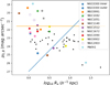 |
Fig. 6. Classification of the sample adapted from Sprayberry et al. (1995), Hagen et al. (2016). The squares symbols represent the value of the disk fit for the inner part of the galaxies and the cross symbols for the extended UV region. The blue line distinguishes the Low Surface Brightness (LSB) galaxies from the Giant LSB (GLSB) galaxies. The orange line, which represents the Freeman (1970) value (21.65 mag.arcsec−2), separates the high surface brightness (HSB) galaxies from the LSB galaxies. In order to compare with the data of McGaugh & Bothun (1994), Sprayberry et al. (1995), and Hagen et al. (2016) (black dots) calculated with H0 = 100 h km s−1 Mpc−1, we corrected the Scalelength with h−1. |
Figure 6 shows that our sample is located in different parts of the Sprayberry diagnostic plot and three families can be distinguished, as described below. The first family is defined as the Malin-1-like galaxies. It is composed of NGC 6902, NGC 1512, and NGC 1140, for which the outer region falls within the GLSB region, while the inner region is in the HSB area. Thus, one third of our XUV galaxies could be considered GLSB galaxies. However, GLSB galaxies are sometimes defined with additional criteria with respect to the Sprayberry plot. For instance, Saburova et al. (2023) add a criteria on their size that is only fulfilled by NGC 6902 among the three galaxies. Zhu et al. (2023) instead use a criteria on the HI mass (above 1010 M⊙) and size (larger than 50 kpc). Only NGC 6902 again is sufficiently massive to be a potential GLSB galaxy according to this definition. The Malin-1-like family described in this paper only refers to the position in the Sprayberry plot, and its diffuseness (see below).
The second family, the regular galaxies, is composed of NGC 1051, NGC 2090, and NGC 0300. The outer central surface brightness (μ0, outer) is fainter than the inner region one, as for the Malin-1-like family, but the outer disk is not in the giant LSB area, with a smaller scale length. The inner and outer values of μ0 and Rs are similar; the profiles do not change much at R25. We also notice that the inner regions of the three galaxies are on the LSB side of the figure (μ0, inner below the Freeman 1970, value).
The last family is made of NGC 1042, NGC 0991, and NGC 1672 for which both the inner and outer regions are in the hight surface brightness (HSB) area and μ0 is fainter in the inner region than in the outer region. We want to stress that the fact that the outer disks fall in the HSB area does not mean that the optical disk is HSB. Actually, by construction, the disks are themselves below 25 mag arcsec−2. A high central surface brightness of μ0, outer is rather indicative of a down-bending profile (Pohlen & Trujillo 2006). In our case, this change is found between the inner disk and the XUV region. We call this family Malin-1-opposite.
Even if our sample is too small to derive definitive conclusions, we note that there is no systematic correlation between the families described above and the XUV type (1 or 2), or the shape of the profile (exponential, up-bending, down-bending) defined by Pohlen & Trujillo (2006), although Malin-1-like galaxies are not down-bending and Malin-1-opposites are not up-bending.
To better characterize optical disks of our sample of XUV galaxies, we used a ‘diffuseness index’ defined by Sprayberry et al. (1995). GLSB galaxies are separated from regular LSB galaxies at a diffuseness index of 27 and designated as
 (3)
(3)
We computed the diffuseness of the outer disk of each galaxy (see Table 2). We found that diffuseness correlates (with some dispersion) both with the scale length and the central surface brightness of the outer disk, which is expected from its definition.
We could not establish any other link with previously measured values such as μ0 or Rs of the inner fit. The diffuseness does not seem to correlate with other global values (mass of gas, integrated g-band luminosity from the profile, either integrated within R25 or RUV, given in Table 2). On average, Type 1, 2, and 1 + 2 XUV galaxies have a mean diffuseness of 26, 23, and 24, respectively. This indicates that type 1 XUV galaxies may be more diffuse in the optical regime than type 2 ones, but the size of our sample is too small to derive strong conclusions on this point.
We also explored whether the difference between the fit values in the inner part and in the outer part could be related to other properties. For truncated galaxies, we expect μ0, inner > μ0, outer and Rs, outer < Rs, inner, while it is the opposite for antitruncated galaxies. We note that this definition is not always in line with the description of the literature of truncated (down-bending) or antitruncated (up-bending) galaxies. This may occur mostly because in our case we are focused on the difference between the XUV area (outer region, R25 < R < RUV) and the disks inside R25 (inner region), while the truncation nature of the profiles in the literature is usually considered on the basis of the full profile, without focusing on a particular radial range.
Again, we did not find any strong correlation that would relate the difference between inner and outer disks to other properties of the galaxies. However, a correlation is expected by definition, once it is noted that the two exponential fits should be continuous at R25, i.e.,

which leads to the relation
 (4)
(4)
where DIS stands for the difference of inverse scale length, defined as

Although the fits are very simple (pure exponential, without decomposition), not perfect and not forced to reach exactly 25 at R25, the values we obtain are consistent with Equation (4), as shown in Fig. 7. The three different families are actually simply separated by their DIS. The Malin-1-opposite are found for negative values, the regular galaxies are found at 0 < DIS < 2. Malin-1-like (and Malin 1) are found above two. Since our galaxies follow Equation (4), the three families are also distinguished by their value of μ0, outer − μ0, inner.
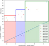 |
Fig. 7. Top: Diffuseness as a function of DIS. Bottom: Difference between the central surface brightness in the outer and inner region as a function of DIS. The blue line represents Equation (4). Each shape corresponds to a XUV family: triangles are Malin-1-opposite; diamonds are Malin-1-like; stars are regular. |
Furthermore, we found a strong correlation between the DIS and the diffuseness of the outer part: the Malin-1-opposite are found under a diffuseness index of 21, the regular galaxies are located between 21 and 27, and the Malin-1-like are above 27. The families we defined can thus be broadly distinguished using only one parameter (e.g., DIS or diffuseness).
We note, however, that this conclusion only applies to the structural properties obtained with the two exponential fits. In the following, we see that NGC 1140 distinguishes itself when the color gradient, stellar age radial variation, or morphology are considered, as discussed in Sect. 4.1.
3.4. Color profile and SED fitting
In this section, we explore the insights that the data can offer into the nature of stellar populations present in the extended UV disks. First, we show the (g − r) color profiles in Figure 8. As expected for star-forming galaxies, in the inner region, we obtain a negative gradient in the (g − r) profiles, except for NGC 1140 (more details of this particular galaxy are given in Section 4.1). Between R25 and RUV, errors become increasingly large with radius and make it difficult to interpret the color profile. However, many of the profiles are constrained well enough at least in some part of the XUV region to suggest a flat blue profile (NGC 991, NGC 1042, NGC 2090, NGC 6902), or are consistent with such a behavior (NGC 300, NGC 1512) within large uncertainties, with the only exception being NGC 1140. This suggests that in most cases the XUV region is relatively recent (and thus blue). In some cases, a few red peaks are found within the UV extended area (e.g., NGC 0991), for which we cannot exclude some contamination being missed despite careful masking. We also observe, in a few cases, a reddening toward the outer edge (e.g., NGC 6902, NGC 1672), which could indicate that we are reaching the stellar halo population, but the uncertainties are always large enough to agree with a flat profile in those cases.
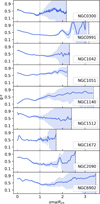 |
Fig. 8. Color profile g − r of the sample. The profiles are corrected for the inclination and galactic extinction. The dashed gray line is the R25 and the black one is the RUV. |
Instead of only using a color profile, we tried to use all available bands of DES and GALEX to constrain the mean age of the underlying stellar population with le Phare (Arnouts et al. 1999; Ilbert et al. 2006) using the GASPIC service1. All details about the input parameters are given in Appendix A.
For each radius of the profiles, the best model of SFR history (SFRmodel) that fits the data is given with the associated age (Agefit) of this model. We then computed the mean stellar age (⟨age⟩) as
 (5)
(5)
While the code can compute uncertainties for some parameters in the Bayesian analysis, we examine the age of the stellar population, which requires knowledge of the star formation history (see Equation (5)). This is given in the best fit model that remains unknown in the Bayesian analysis. Therefore, to estimate the errors, we created 100 mocks for each radius using a normal distribution of the observed uncertainties. For each of the mock, le Phare again gives the best model and age, and a mean age by using Equation (5). We computed the quartiles, the median, the minimum, and maximum age. In addition, we created histograms of the age distribution each 20 arcsec (with a bin around 1 Gyr) in order to measure the mode of the distribution. We found that the distribution is wide (not bringing a strong constraint on ⟨age⟩), very asymmetric, with a mode close to the value we found, but lower than the median of the mocks (see Fig. A.1 of Appendix A). This probably arises because the models are largely degenerated, with only seven bands and relatively large uncertainties in the outer parts. Nevertheless, we can try to derive broad trends, keeping these caveats in mind.
Most of the galaxies in the sample present an age gradient in the inner region as shown in Fig. A.1, despite some variability, and are in most cases consistent with young ages in the outer region (e.g., NGC 0300, NGC 1042, NGC 1672, NGC 2090). This indication of recent formation in the outer regions is consistent with the conclusion from the color profiles (Fig. 8). For several galaxies, there are peaks of older age in the outer part of the galaxies with the data or in some mock values (e.g., NGC 0991, NGC 1051, NGC 6902). Although it is difficult to assess the precise reason, it illustrates again that some degeneracy remains with the current data.
On the contrary, NGC 1140 presents a very old stellar population in the outer disk just beyond R25, and a very young one in the inner disc. This is consistent with the color gradient discussed above. Even if some other galaxies do present some peaks of old stellar population in some parts of the extended disk (that are hard to interpret considering the uncertainties), the case of NGC 1140 remains unique and is discussed in Section 4.1.
Concerning the SED-fiting, le Phare provides the Chi2 that are quite low, which indicates that our uncertainties may be overestimated (we indeed decided to be conservative, see Sect. 2.2). In order to test the reproducibility of our results, we also calculated ⟨age⟩ with Cigale (Boquien et al. 2019), and applied a similar method (and the input parameter given in Appendix A). The values obtained with Cigale are very similar to le Phare in most cases, with some differences sometimes at the largest radii (within the range of models found in our mocks). These results based on SED fitting must be interpreted with caution, especially due to the large uncertainties, in the outer regions in particular. To improve our results in the future, we would need more bands and better image quality (especially a better sky background that would allow us to reduce the uncertainties of the photometry).
4. Discussions
4.1. The different formation of the XUV extended structure in NGC 1140
In Sect. 3.3.2, we could not distinguish NGC 1140 from the rest of the sample based on the pure structural properties of the optical extended disk. We found it to be Malin-1-like, with a strong antitruncation in the XUV region. However, the color profile was found to be peculiar, with a reddening from the center outward, contrary to the rest of the sample. In Sect. 3.4, the SED fitting indicated the presence of an old stellar population beyond R25, and a very recent one in the inner part, contrary to the rest of the sample again.
Inspection of the morphology of the galaxy may help to understand these differences. Indeed, the other galaxies present spiral arms and knots in the outer disk, which strongly suggests star formation in an extended gas disk, while NGC 1140 exhibits a very irregular morphology, which is expected from its type, T = 9 (Thilker et al. 2007), but also shells that are clearly visible in the DES images (see Fig. 9). We verified that we do not see more structures than the one visible in this figure, once the image is masked and binned.
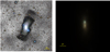 |
Fig. 9. NGC 1140 with DES data. Left: NGC 1140 color image with g band, r band, and i band of DES. Right: Zoom on the double nucleus. |
Such shells usually indicate a recent merger (e.g., Zhang et al. 2020a, and references within), even if they are more usually found in early-type systems. Signs of mergers for NGC 1140 had already been found, such as the presence and morphology of Hα regions, and super star clusters (Hunter et al. 1994; Westmoquette et al. 2010), but the shells were not known up to now to our knowledge. The morphology of the system is very similar to that of VCC 848 observed by Zhang et al. (2020b), which was interpreted as the sign of a recent (rarely observed) dwarf-dwarf merger. Both galaxies are irregular blue compact dwarf galaxies (BCD) as established by Zhang et al. (2020a) and Wu et al. (2008). In NGC 1140, a double nucleus is still present (see Figure 9), while in VCC 848 there is no sign of the secondary component that has been completely disrupted (Zhang et al. 2020a). It has been suggested that Ark18, with a blue extended LSB disk presenting some similitudes with GLSB galaxies could also results from a dwarf-dwarf merger (Egorova et al. 2021).
These observations of NGC 1140 and VCC 848 are consistent with the simulations of Bekki (2008) showing that the merger of dwarf-rich dIrr galaxies can result in a BCD, and eventually a dIrr with spherical structures in the outer parts, which could correspond to the old ages found outward of R25 in our case. While studies of the mergers of dwarf galaxies are rare, NGC 1140 and VCC 848 are probably two very good examples, with deep optical data allowing the detection of the shells and old stellar population in the outskirts, and an extended gas distribution. In another study on the formation of BCD galaxies via dwarf mergers, Chhatkuli et al. (2023) target a few BCDs from a catalog of dwarf merger galaxies (Paudel et al. 2018) on the basis of interaction features such as the tidal structure or shells seen in SDSS images. NGC 1140 was not in this sample, as it is not in the SDSS footpath.
In Table 3, we provide the values for the stellar mass, gas mass, SFR, and light distribution of NGC 1140, VCC 848, and the six BCDs of Chhatkuli et al. (2023). For all galaxies in this table, we computed the scale length and the central surface brightness in the inner part as in Section 3.1 in order to find connections between those galaxies and NGC 1140. The values for NGC 1140 are within the observed range for the other galaxies. The most similar galaxy is D075: both are relatively massive dwarfs, with a large gas reservoir.
Properties of NGC 1140 and other BCD galaxies resulting from dwarf-dwarf mergers from Zhang et al. (2020a) and Chhatkuli et al. (2023).
Zhang et al. (2020b) found VCC 848 to be above the main sequence using Shin et al. (2020) as a reference. Our determined SFR (4.2 M⊙/yr) places NGC 1140 even more above the main sequence, probably resulting from a temporary enhancement of star formation during the merger phase (it may be a reason for the XUV classification). Westmoquette et al. (2010) provided a SFR of 0.7 M⊙/yr, smaller than ours but determined from Hα, which is more sensitive to small timescale variations and dominated by few regions of intense star formation, while our SED fitting is constrained by the UV emission in an extended area, which is sensitive to longer timescales. For its stellar mass, NGC 1140 is also one of the most gas-rich dwarfs compared to other dwarfs, using Henkel et al. (2022) as a reference, which makes it an extreme case in its category.
4.2. Euclid perspectives
Euclid offers new possibilities, as it offers a very large sky coverage and exquisite resolution. The ERO (Early Release Observations) images (Cuillandre et al. 2025) especially were processed in such a way as to keep the LSB signal. Among the six galaxies in the sample studied with Euclid by Hunt et al. (2025), one (NGC 2403) was classified as an XUV galaxy in Thilker et al. (2007). We thus performed a similar analysis to the one made for our sample. We fit the profiles of Hunt et al. (2025) in the wide Ie Euclid band, and used the GALEX images to find the RUV as in Sect. 3.3.1 (RUV = 912 arcsec andR25 = 594 arcsec).
To compare this galaxy observed in IE to our sample in the g band, we compared the Ie profile with the profile in Barker et al. (2012) in the V band and then applied the (V-B) correction of Fukugita et al. (1995). This allowed us to add this galaxy to our figures (see Figs. 6 and 7).
Following the procedure of Sect. 3.3.2, we found that NGC 2403 is part of the regular family, but with a brighter surface brightness than the three other galaxies of its category. This shows the potential of Euclid to study XUV galaxies. Urbano et al. (2025) discuss the use of ERO data (and Euclid in the future) to study other LSB structures (especially traces of the past assembly of galaxies such as tails and shells). With stray light problems reduced in the future with respect to ERO data, Euclid has the potential for new discoveries in LSB science, although the impact of the different pipeline between ERO and regular observations will have to be determined.
5. Conclusions
For a sample of nine XUV galaxies, we used available deep optical images from DES, in combination with UV images from GALEX in order to characterize their UV-emitting outer disk in the optical wavelength. The main objective was to conduct a comparative analysis with the GLSB galaxies, which are typically defined based on optical data (here, we call “GLSB galaxies” as galaxies with a very large diffuseness, as defined by Sprayberry et al. (1995), which are not necessarily very massive or extremely large).
For this, we first defined a physically based UV radius, RUV. We then proposed fitting the g-band profile in the inner (R < R25) and outer disk (R25 < R < RUV) in order to analyze the structural properties of these galaxies. This led us to distinguish three different families of XUV galaxies: (i) the Malin-1-like family represents the galaxies for which the outer region fit parameters place them in the GLSB region in the diagnostic figure of Sprayberry et al. (1995), similarly to the most extreme GLSB galaxy, Malin-1 (independently of their gas content and physical size). (ii) Malin-1-opposite is a family for which the central surface brightness extrapolated from the fit of the inner region is fainter than that of the outer disk, which corresponds to a steeper slope in the outer regions than in the inner regions, contrary to the Malin-1 archetype of GLSB galaxies. (iii) We dubbed regular galaxies the rest of the sample, for which the extrapolated central surface brightness of the outer disk is fainter than that of the inner region (like GLSB galaxies), but the outer disk scale length is too small to fall into the GLSB region. XUV galaxies are therefore far from all being similar to GLSB galaxies. These three families can be simply distinguished by the variable DIS (see Equation (4)) or the diffuseness index of the outer part (see Fig. 7), which goes from truncated profiles to strongly antitruncated profiles similar to Malin-1 and the GLSB galaxies.
However, our work also demonstrates that this structural property determined with only one band is not sufficient to completely describe the outer disk for the full sample of XUV galaxies. The positive g − r color gradient distinguishes one of our nine galaxies (NGC 1140). Analyses of the morphology and the stellar population strongly suggest this galaxy results from a recent merger. Its XUV nature is due to young regions, but at the same time an old stellar population is found in outer shells clearly visible in the DES images. The rest of the sample (eight out of nine galaxies) presents a negative color gradient and are rather giant star-forming disks, more similar to giant LSBs, but with a variety of profiles types (antitruncated to truncated).
In the future, many opportunities for studying XUV (and LSB) galaxies will arise. We showed that EUCLID may allow us to study many XUV galaxies considering its large sky overage, if a pipeline adapted to extended faint objects is used, as is done in the ERO observations, in which one XUV galaxy was observed (NGC 2403). This galaxy was found to correspond to our regular galaxy family but is brighter than the other members. We clearly need to enlarge the sample of XUV galaxies studied in optical to verify that our proposed families are adequate to describe all XUV galaxies to better characterize them and refine our classification. Other sky surveys that may bring a large amount of data for this are the large multiwavelength surveys that will reach depths down to 30 mag arcsec−2 like LSST (Ivezić et al. 2019) or the Ultraviolet Near-Infrared Optical Northern Survey (UNIONS)2. Another opportunity will be the use of dedicated telescopes like Calar Alto Schmidt Lemaître Telescope (CASTLE) (Lombardo et al. 2019; Muslimov et al. 2017), which will cover large fields with an excellent sky background, PFS, and low contamination. It will help us to characterize the outer regions of XUV galaxies and their stellar population for dedicated targets, especially the largest among XUV galaxies.
Data availability
Profiles from Figure 2 are only available in electronic form at the CDS via anonymous ftp to https://cdsarc.cds.unistra.fr/viz-bin/cat/J/A+A/700/A56
Acknowledgments
This work is partly based on tools and data products produced by GAZPAR operated by CeSAM-LAM and IAP. We thank Simona Lombardo for her help in early phases of this work, and the information she provided in the context of the CASTLE project. E.B would like to acknowledges the meaningful discussions with Mathias Urbano and his support. J. is funded by the European Union (MSCA EDUCADO, GA 101119830 and WIDERA ExGal-Twin, GA 101158446). This work was supported by the ≪ action thématique ≫ Cosmology-Galaxies (ATCG) of the CNRS/INSU PN Astro. This work was partially supported by the “PHC POLONIUM” program (project number: 49136QB), funded by the French Ministry for Europe and Foreign Affairs, the French Ministry for Higher Education and Research and the Polish National Agency for Academic Exchange “POLONIUM” grant BPN/BFR/2022/1/00005.
References
- Abazajian, K. N., Adelman-McCarthy, J. K., Agüeros, M. A., et al. 2009, ApJS, 182, 543 [Google Scholar]
- Abbott, T. M. C., Adamów, M., Aguena, M., et al. 2021, ApJS, 255, 20 [NASA ADS] [CrossRef] [Google Scholar]
- Argence, B., & Lamareille, F. 2009, A&A, 495, 759 [NASA ADS] [CrossRef] [EDP Sciences] [Google Scholar]
- Arnouts, S., Cristiani, S., Moscardini, L., et al. 1999, MNRAS, 310, 540 [Google Scholar]
- Barker, M. K., Ferguson, A. M. N., Irwin, M. J., Arimoto, N., & Jablonka, P. 2012, MNRAS, 419, 1489 [CrossRef] [Google Scholar]
- Barth, A. J. 2007, AJ, 133, 1085 [NASA ADS] [CrossRef] [Google Scholar]
- Bekki, K. 2008, MNRAS, 388, L10 [Google Scholar]
- Bigiel, F., Leroy, A., Walter, F., et al. 2008, AJ, 136, 2846 [NASA ADS] [CrossRef] [Google Scholar]
- Boissier, S. 2013, in Extragalactic Astronomy and Cosmology, eds. T. D. Oswalt, & W. C. Keel, Planets, Stars and Stellar Systems, 6, 141 [Google Scholar]
- Boissier, S., Gil de Paz, A., Boselli, A., et al. 2008, ApJ, 681, 244 [NASA ADS] [CrossRef] [Google Scholar]
- Boissier, S., Boselli, A., Ferrarese, L., et al. 2016, A&A, 593, A126 [NASA ADS] [CrossRef] [EDP Sciences] [Google Scholar]
- Boquien, M., Burgarella, D., Roehlly, Y., et al. 2019, A&A, 622, A103 [NASA ADS] [CrossRef] [EDP Sciences] [Google Scholar]
- Bothun, G. D., Impey, C. D., Malin, D. F., & Mould, J. R. 1987, AJ, 94, 23 [NASA ADS] [CrossRef] [Google Scholar]
- Bothun, G., Impey, C., & McGaugh, S. 1997, PASP, 109, 745 [NASA ADS] [CrossRef] [Google Scholar]
- Bouquin, A. Y. K., Gil de Paz, A., Muñoz-Mateos, J. C., et al. 2018, ApJS, 234, 18 [NASA ADS] [CrossRef] [Google Scholar]
- Bradley, L., Sipőcz, B., Robitaille, T., et al. 2024, https://doi.org/10.5281/zenodo.10967176 [Google Scholar]
- Bruzual, G., & Charlot, S. 2003, MNRAS, 344, 1000 [NASA ADS] [CrossRef] [Google Scholar]
- Cardelli, J. A., Clayton, G. C., & Mathis, J. S. 1989, ApJ, 345, 245 [Google Scholar]
- Chabrier, G. 2003, PASP, 115, 763 [Google Scholar]
- Chhatkuli, D. N., Paudel, S., Bachchan, R. K., Aryal, B., & Yoo, J. 2023, MNRAS, 520, 4953 [Google Scholar]
- Cuillandre, J. C., Bertin, E., Bolzonella, M., et al. 2025, 2025, A&A, 697, A6 [Google Scholar]
- Disney, M. J. 1976, Nature, 263, 573 [Google Scholar]
- Draine, B. T., & Li, A. 2007, ApJ, 657, 810 [CrossRef] [Google Scholar]
- Egorova, E. S., Egorov, O. V., Moiseev, A. V., et al. 2021, MNRAS, 504, 6179 [CrossRef] [Google Scholar]
- Euclid Collaboration (Mellier, Y., et al.) 2025, A&A, 697, A1 [Google Scholar]
- Freeman, K. C. 1970, ApJ, 160, 811 [Google Scholar]
- Fukugita, M., Shimasaku, K., & Ichikawa, T. 1995, PASP, 107, 945 [Google Scholar]
- Gil de Paz, A., & Madore, B. F. 2005, ApJS, 156, 345 [NASA ADS] [CrossRef] [Google Scholar]
- Gil de Paz, A., Madore, B. F., Boissier, S., et al. 2005, ApJ, 627, L29 [Google Scholar]
- Gil de Paz, A., Boissier, S., Madore, B. F., et al. 2007, ApJS, 173, 185 [Google Scholar]
- Hagen, L. M. Z., Seibert, M., Hagen, A., et al. 2016, ApJ, 826, 210 [NASA ADS] [CrossRef] [Google Scholar]
- Haslbauer, M., Banik, I., Kroupa, P., & Grishunin, K. 2019, MNRAS, 489, 2634 [NASA ADS] [CrossRef] [Google Scholar]
- Henkel, C., Hunt, L. K., & Izotov, Y. I. 2022, Galaxies, 10, 29 [Google Scholar]
- Hunt, L. K., Annibali, F., Cuillandre, J. C., et al. 2025, A&A, 697, A9 [NASA ADS] [CrossRef] [EDP Sciences] [Google Scholar]
- Hunter, D. A., O’Connell, R. W., & Gallagher, J. S., III 1994, AJ, 108, 84 [Google Scholar]
- Ilbert, O., Arnouts, S., McCracken, H. J., et al. 2006, A&A, 457, 841 [NASA ADS] [CrossRef] [EDP Sciences] [Google Scholar]
- Ivezić, Ž., Kahn, S. M., Tyson, J. A., et al. 2019, ApJ, 873, 111 [Google Scholar]
- Junais, Boissier, S., Boselli, A., et al. 2021, A&A, 650, A99 [NASA ADS] [CrossRef] [EDP Sciences] [Google Scholar]
- Junais, Weilbacher, P. M., Epinat, B., et al. 2024, A&A, 681, A100 [NASA ADS] [CrossRef] [EDP Sciences] [Google Scholar]
- Kennicutt, R. C., Jr. 1998, ApJ, 498, 541 [Google Scholar]
- Koda, J., Yagi, M., Yamanoi, H., & Komiyama, Y. 2015, ApJ, 807, L2 [NASA ADS] [CrossRef] [Google Scholar]
- Kravtsov, A. 2024, Open J. Astrophys., accepted [arXiv:2406.13732] [Google Scholar]
- Kroupa, P. 2001, MNRAS, 322, 231 [NASA ADS] [CrossRef] [Google Scholar]
- Lelli, F., Fraternali, F., & Sancisi, R. 2010, A&A, 516, A11 [NASA ADS] [CrossRef] [EDP Sciences] [Google Scholar]
- Lombardo, S., Muslimov, E., Lemaître, G., & Hugot, E. 2019, MNRAS, 488, 5057 [Google Scholar]
- Martin, G., Kaviraj, S., Laigle, C., et al. 2019, MNRAS, 485, 796 [NASA ADS] [CrossRef] [Google Scholar]
- McGaugh, S. S., & Bothun, G. D. 1994, AJ, 107, 530 [NASA ADS] [CrossRef] [Google Scholar]
- McGaugh, S. S., & de Blok, W. J. G. 1998, ApJ, 499, 41 [CrossRef] [Google Scholar]
- McGaugh, S. S., Bothun, G. D., & Schombert, J. M. 1995, AJ, 110, 573 [Google Scholar]
- Merritt, A., Dokkum, P. v., Abraham, R., & Zhang, J. 2016, ApJ, 830, 62 [Google Scholar]
- Mihos, J. C., Durrell, P. R., Ferrarese, L., et al. 2015, ApJ, 809, L21 [Google Scholar]
- Minchin, R. F., Disney, M. J., Parker, Q. A., et al. 2004, MNRAS, 355, 1303 [NASA ADS] [CrossRef] [Google Scholar]
- Monnier Ragaigne, D., van Driel, W., Balkowski, C., Boissier, S., & Prantzos, N. 2003, Ap&SS, 284, 917 [Google Scholar]
- Morrissey, P., Schiminovich, D., Barlow, T. A., et al. 2005, ApJ, 619, L7 [CrossRef] [Google Scholar]
- Muslimov, E., Valls-Gabaud, D., Lemaître, G., et al. 2017, Appl. Opt., 56, 8639 [Google Scholar]
- O’Neil, K., & Bothun, G. 2000, ApJ, 529, 811 [CrossRef] [Google Scholar]
- Paudel, S., Smith, R., Yoon, S. J., Calderón-Castillo, P., & Duc, P.-A. 2018, ApJS, 237, 36 [Google Scholar]
- Pohlen, M., & Trujillo, I. 2006, A&A, 454, 759 [NASA ADS] [CrossRef] [EDP Sciences] [Google Scholar]
- Robitaille, T., Ginsburg, A., Mumford, S., et al. 2023, https://doi.org/10.5281/zenodo.7584411 [Google Scholar]
- Saburova, A. S., Chilingarian, I. V., Katkov, I. Y., et al. 2018, MNRAS, 481, 3534 [CrossRef] [Google Scholar]
- Saburova, A. S., Chilingarian, I. V., Kasparova, A. V., et al. 2021, MNRAS, 503, 830 [NASA ADS] [CrossRef] [Google Scholar]
- Saburova, A. S., Chilingarian, I. V., Kulier, A., et al. 2023, MNRAS, 520, L85 [Google Scholar]
- Shin, K., Ly, C., Malkan, M. A., et al. 2020, MNRAS, 501, 2231 [Google Scholar]
- Sprayberry, D., Impey, C. D., Bothun, G. D., & Irwin, M. J. 1995, AJ, 109, 558 [NASA ADS] [CrossRef] [Google Scholar]
- Thilker, D. A., Bianchi, L., Meurer, G., et al. 2007, ApJS, 173, 538 [Google Scholar]
- Trujillo, I., D’Onofrio, M., Zaritsky, D., et al. 2021, A&A, 654, A40 [NASA ADS] [CrossRef] [EDP Sciences] [Google Scholar]
- Urbano, M., Duc, P. A., Saifollahi, T., et al. 2025, A&A, in press, https://doi.org/10.1051/0004-6361/202453534 [Google Scholar]
- van Dokkum, P. G., Abraham, R., Merritt, A., et al. 2015, ApJ, 798, L45 [NASA ADS] [CrossRef] [Google Scholar]
- Westmoquette, M. S., Gallagher, J. S., & de Poitiers, L. 2010, MNRAS, 403, 1719 [NASA ADS] [CrossRef] [Google Scholar]
- Wu, Y., Charmandaris, V., Houck, J. R., et al. 2008, ApJ, 676, 970 [Google Scholar]
- Yagi, M., Koda, J., Komiyama, Y., & Yamanoi, H. 2016, ApJS, 225, 11 [CrossRef] [Google Scholar]
- Zhang, H.-X., Paudel, S., Smith, R., et al. 2020a, ApJ, 891, L23 [CrossRef] [Google Scholar]
- Zhang, H.-X., Smith, R., Oh, S.-H., et al. 2020b, ApJ, 900, 152 [NASA ADS] [CrossRef] [Google Scholar]
- Zhu, Q., Pérez-Montaño, L. E., Rodriguez-Gomez, V., et al. 2023, MNRAS, 523, 3991 [NASA ADS] [CrossRef] [Google Scholar]
- Zwaan, M. A., van der Hulst, J. M., de Blok, W. J. G., & McGaugh, S. S. 1995, MNRAS, 273, L35 [NASA ADS] [Google Scholar]
Appendix A: SED-Fitting
To derive the physical properties of our sources, we performed SED fitting using two tools in the astrophysical community: Le Phare and CIGALE. Both were accessed through the GAZPAR interface. We used the profiles described in Sec 2.2. It is apparent that the resolution of GALEX (about 4.5 arcsec) differs from that of DES (0.263 arcsec). However, the application of a 13x13 binning to the reprojection of GALEX onto the DES pixel results in a final pixel of 3.4 arcsec, which is comparable to the resolution of GALEX. Since we are interested in profiles along big ellipses in these large pixels, the resolution mismatch has little effect, especially at large radii where the profiles are relatively flat. We performed nevertheless a convolution of all the images with a Gaussian Kernel to match the GALEX resolution at all wavelengths. As expected, we found that the profiles remain similar but that this method introduces complexities, as some sources in the DES data that pollutes a larger area. This makes the masking process and sky determination more difficult, increasing the uncertainties in the outer part of the profiles. We thus decided to use the profiles obtained with a 3.4 arcsec binning without this convolution.
A.1. Le Phare Configuration
The first modeling run was conducted using Le Phare, as described in Arnouts et al. (1999) and Ilbert et al. (2006). The SED fitting relies on the Bruzual & Charlot (2003) stellar population synthesis models, assuming a Chabrier (2003) IMF. The star formation histories are modeled with exponentially delayed model. The dust attenuation is parameterized by the redenning E(B − V), varied over a grid: 0.0, 0.05, 0.1, 0.15, 0.2, 0.25, and 0.3.
We adopt a ΛCDM cosmology with H0 = 70 km s−1 Mpc−1, Ωm = 0.3, and ΩΛ = 0.7. The redshift range is limited to a maximum of 0.006, sampled in steps of 0.001. The DES g-band is selected as the reference band for normalization. Default values were retained for photometric error adjustments and rescaling factors across the photometric bands. The result of this fit is shown in the Figure A.1
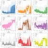 |
Fig. A.1. Mean age as a function of the radius. The dotted line is the mean age calculated with Le Phare and the continuous line is the median of the mock simulations (see section 3.4). The triangles represent the mode of the mean age of the mocks in a range of 20 arcsec. The gray dotted line is the R25 while the black one is the RUV. The shadow area is the area between the first and the third quartile of the mocks while the light area is the minimum and the maximum mean age found in the mocks. |
A.2. CIGALE Configuration
We also used CIGALE (Boquien et al. 2019) to perform an other SED fitting. This run uses the BC03 stellar population models based on Chabrier (2003) IMF, and a delayed star formation history module. Dust emission is treated with the dl2014 module (Draine & Li 2007). No AGN or radio emission components are included in this analysis.
The tau main (τ) for the SFH is explored in three values: 100, 5000, and 10000 Myr. We fixed only three values to constraint the age. The stellar population ages range from very young to old populations: starting with fine steps (10, 20, 50 Myr), then gradually increasing every 100 Myr between 100 and 1000 Myr, every 200 Myr between 1000 and 2000 Myr, every 500 Myr up to 5000 Myr, and finally every 1000 Myr until 13000 Myr. This allows coverage of a wide temporal baseline suitable for tracing the evolution of various stellar populations.
The color excess for young stellar populations, E(B − V)young, spans the same grid as in Le Phare. For the older populations, the reduction factor is set to 0.5. We adopted a low metallicity value of Z = 0.004, consistent with expectations for low densities in the outer regions.
Attenuation parameters include a fixed UV bump amplitude of 3.0 and an attenuation law slope of 0. All other parameters were left unchanged from their default settings in CIGALE.
All Tables
Properties of NGC 1140 and other BCD galaxies resulting from dwarf-dwarf mergers from Zhang et al. (2020a) and Chhatkuli et al. (2023).
All Figures
|
Fig. 1. DES images of the sample in g band. The ellipses show the adopted position angle and ellipticity at the R25 (RUV) radius in red (green). |
| In the text | |
|
Fig. 2. Observed surface brightness profiles for each band of the sample as a function of the semimajor axis of the ellipses. The dashed gray line is the R25 and the dashed black line is the RUV defined in Section 3.3.1. For clarity, an offset have been applied on the profiles of +n magnitudes/arcsec2 with a dependence on the bands indicated in the bottom right panel. The dotted blue line represents 25 mag.arcsec−2 in the B band adapted to the g band using Fukugita et al. (1995). |
| In the text | |
|
Fig. 3. Surface brightness profile in g band for NGC 1042 as a function of the semimajor axis (sma) of ellipses. Top: Comparison of the method with the profile from Trujillo et al. (2021) with LBT data (in red) and our method applied to the same data (in green), and the difference between them under the main panel. Bottom: Comparison of the data with the profile from Trujillo et al. (2021) with LBT data (in red), the profile from Merritt et al. (2016) with Dragonfly data, and our method applied to DES data (in blue). The differences between the other profiles and ours are shown under the main panel. The dashed gray line is the R25 of the galaxy when the dashed black line is the RUV. The shaded area shows the uncertainties for LBT data with the method used here in the top panel and DES data with the method used here in the bottom panel. |
| In the text | |
|
Fig. 4. Star formation rate surface density (ΣSFR) as a function of the semimajor axis normalized to the R25. The dashed gray line is the value that corresponds to the RUV. |
| In the text | |
|
Fig. 5. Surface brightness profiles in g band of the sample as a function of the radius normalized by R25. The dashed gray line is the R25 and the black one is the RUV. The dotted green line is the fit in the outer region and the dotted red line is the fit in the inner region. |
| In the text | |
|
Fig. 6. Classification of the sample adapted from Sprayberry et al. (1995), Hagen et al. (2016). The squares symbols represent the value of the disk fit for the inner part of the galaxies and the cross symbols for the extended UV region. The blue line distinguishes the Low Surface Brightness (LSB) galaxies from the Giant LSB (GLSB) galaxies. The orange line, which represents the Freeman (1970) value (21.65 mag.arcsec−2), separates the high surface brightness (HSB) galaxies from the LSB galaxies. In order to compare with the data of McGaugh & Bothun (1994), Sprayberry et al. (1995), and Hagen et al. (2016) (black dots) calculated with H0 = 100 h km s−1 Mpc−1, we corrected the Scalelength with h−1. |
| In the text | |
|
Fig. 7. Top: Diffuseness as a function of DIS. Bottom: Difference between the central surface brightness in the outer and inner region as a function of DIS. The blue line represents Equation (4). Each shape corresponds to a XUV family: triangles are Malin-1-opposite; diamonds are Malin-1-like; stars are regular. |
| In the text | |
|
Fig. 8. Color profile g − r of the sample. The profiles are corrected for the inclination and galactic extinction. The dashed gray line is the R25 and the black one is the RUV. |
| In the text | |
|
Fig. 9. NGC 1140 with DES data. Left: NGC 1140 color image with g band, r band, and i band of DES. Right: Zoom on the double nucleus. |
| In the text | |
|
Fig. A.1. Mean age as a function of the radius. The dotted line is the mean age calculated with Le Phare and the continuous line is the median of the mock simulations (see section 3.4). The triangles represent the mode of the mean age of the mocks in a range of 20 arcsec. The gray dotted line is the R25 while the black one is the RUV. The shadow area is the area between the first and the third quartile of the mocks while the light area is the minimum and the maximum mean age found in the mocks. |
| In the text | |
Current usage metrics show cumulative count of Article Views (full-text article views including HTML views, PDF and ePub downloads, according to the available data) and Abstracts Views on Vision4Press platform.
Data correspond to usage on the plateform after 2015. The current usage metrics is available 48-96 hours after online publication and is updated daily on week days.
Initial download of the metrics may take a while.