© The Authors 2025

1. Introduction

Massive stars (those with an initial mass ≳8 M_⊙) end their lives in a core-collapse (CC) event, possibly with an associated bright supernova (SN) explosion or gamma-ray burst, that results in a compact object, either a neutron star (NS) or a black hole (BH). The majority of massive stars are now known to be born in binaries or higher multiplicity systems, with the multiplicity fraction of stars with M ≳ 10 M_⊙ approaching 100% (Sana et al. 2012; Moe & Di Stefano 2017; Offner et al. 2023). During compact object formation, asymmetries in the SN ejecta can drive a momentum recoil, or “natal kick”, in the remnant, potentially resulting in high velocity compact objects (Katz 1975; Brisken et al. 2003; Hobbs et al. 2005; Verbunt et al. 2017). In binary systems, even symmetric mass loss alone with no additional natal kick (often referred to as a “Blaauw kick”) can significantly modify the orbit or result in isolated compact objects (Blaauw 1961).

Presently, the kicks that stellar-mass BHs attain upon birth represent a major source of uncertainty in stellar evolution modeling, with implications for the formation of stellar binaries containing BHs (Mandel 2016), retention of BHs in globular clusters (Antonini & Gieles 2020), the velocity of dark lenses (Wyrzykowski & Mandel 2020), the mass distribution of massive runaway stars (Dray et al. 2006; Renzo et al. 2019), and the properties of merging binary BHs (Callister et al. 2021; Broekgaarden et al. 2022).

Estimating BH natal kicks is challenging due to the inherent difficulty of detecting BHs in general. Most stellar mass BHs are discovered in binary systems, often as low- or high-mass XRBs. Low-mass XRBs may be very old, and therefore estimating the natal kick requires tracing the system back through its Galactic orbit (Nagarajan & El-Badry 2025) while assuming that the binary formed near the disk and was unperturbed by third-body encounters in the interim. Furthermore, this method can only constrain the full systemic velocity following the CC and cannot disentangle the effects of the natal kick, mass loss, or any pre-collapse systemic velocity (Atri et al. 2019). High-mass XRBs, by contrast, are constrained by the age of the visible companion to be relatively young, and they are thus more likely to have a velocity that reflects their speed immediately following the CC event, although rejuvenation during mass accretion may modify this age constraint. Mirabel & Rodrigues (2003) used the proper motion of the high-mass XRB Cyg X-1 to argue that its low systemic velocity, relative to its presumed birth association (Cygnus OB3), was indicative of a small natal kick and minimal mass loss. Since larger kicks are more likely to disrupt binaries, BHs observed in binaries are evidence that at least some BHs form with weak kicks. Consequently, kick distributions estimated from XRBs are intrinsically biased against larger kicks (Repetto et al. 2012; Mandel 2016; Renzo et al. 2019; Andrews & Kalogera 2022; O’Doherty et al. 2023; Kimball et al. 2023; Burdge et al. 2024; Dashwood Brown et al. 2024).

In addition to constraints from BHs born in isolated binaries, the existence of BHs in globular clusters (e.g., Baumgardt et al. 2019; Weatherford et al. 2020; Dickson et al. 2024) provides evidence that at least some BHs receive kicks that have a value less than the cluster escape velocity. The central escape velocity of Milky Way globular clusters is typically on the order of ∼20 km s⁻¹ at the present day, and it could have been higher by a factor of a few at the time of BH formation due to cluster mass loss and expansion over time (Baumgardt & Hilker 2018). However, due to dynamical interactions within the cluster, the present-day velocity of a cluster BH may be very different from its natal kick, so we cannot infer the natal kicks on a per-system basis.

The mass distribution of runaway massive stars is also sensitive to BH natal kicks. If BH progenitors typically have more massive companions, then larger BH kicks imply more massive runaways, and this can provide a statistical constraint on the kicks as a function of the initial mass ratio distribution, even in the absence of an observed core-collapse or BH (Renzo et al. 2019).

Studies of weak NS natal kicks face similar challenges due to the dynamical effects in clusters and the evolutionary effects on the orbit of NSs in NS-XRBs (O’Doherty et al. 2023). However, transverse velocity observations of hundreds of isolated radio pulsars provide evidence that typical NS natal kicks follow a Maxwellian distribution with scale parameter σ = 265 km s⁻¹ (Hobbs et al. 2005). As a complement to NSs in intact binaries, isolated pulsar velocities are naturally biased toward stronger kicks, and different studies disagree on the magnitude and shape of the low velocity end of the NS natal kick distribution (Arzoumanian et al. 2002; Podsiadlowski et al. 2005; Igoshev et al. 2021; Willcox et al. 2021; Fortin et al. 2022; Zhao et al. 2023).

Unlike radio pulsars, isolated BHs cannot be observed directly, although microlensing provides a method to infer their velocities. The only confirmed detection of a microlensed stellar-mass BH with a velocity constraint is OGLE-2011-BLG-0462/MOA-2011-BLG-191 (Sahu et al. 2022; Lam et al. 2022). Although the original nature and properties of OGLE-2011-BLG-0462/MOA-2011-BLG-191 were disputed (Mróz et al. 2022), subsequent analysis has confidently placed the BH mass between ∼6 − 8 M_⊙ and the transverse velocity at ≲45 km s⁻¹ (Sahu et al. 2022; Mróz et al. 2022), with an estimated BH natal kick of ≲100 km s⁻¹ (Andrews & Kalogera 2022). Based on the observed rate of microlensing events, Koshimoto et al. (2024) estimate that the average kick velocity of isolated BHs should be ≲100 km s⁻¹. However, in this analysis we did not account for the likelihood that the BHs observed in microlensing events are most likely of binary origin (Vigna-Gómez & Ramirez-Ruiz 2023).

A promising yet computationally costly alternative to study BH natal kicks comes from 3D SN simulations (Janka et al. 2016, 2022; Müller 2020; Mezzacappa 2023; Wang et al. 2022). While some recent studies have argued that most BHs receive kicks < 100 km s⁻¹ (Coleman & Burrows 2022), others have shown that some newly formed BHs may attain kicks larger than 1000 km s⁻¹ at least at some point during the explosion (Burrows et al. 2023, 2024; Janka & Kresse 2024). These extreme values are expected to reduce with the accretion of fallback material from the envelope (Schrøder et al. 2018; Chan et al. 2020). However, simulating for long enough to resolve these later phases is just at the edge of the computational capabilities of current simulations, and systematic trends are presently out of reach. As such, there is no clear consensus from 3D modeling on the magnitude of BH kicks and their dependence on the properties of the progenitor.

Recent discoveries of a new population of inert black hole binaries (BHBs) provide a promising new window into BH formation and direct constraints on natal kicks and mass loss (Shenar et al. 2022a). Also referred to as “detached” or “dormant”, inert BHBs are composed of a BH and a nondegenerate star, with no observed X-ray emission or signatures of an accretion disk. The term “inert” distinguishes these from quiescent XRBs, which fluctuate between X-ray emitting and X-ray quiet (see Hirai & Mandel 2021; Sen et al. 2024 for discussions). The persistent lack of X-rays characterizes these systems as wide, noninteracting binaries. Some are detected spectroscopically, such as the binary in NGC 3201 (Giesers et al. 2018), the Galactic binary HD 130298 (Mahy et al. 2022), and the LMC binary VFTS 243 (Shenar et al. 2022a). Others, such as the three Gaia BHs, have been detected via astrometry and were later confirmed spectroscopically as inert BHBs (El-Badry et al. 2023a,b; Chakrabarti et al. 2023; Tanikawa et al. 2023; Gaia Collaboration 2024). Additionally, several candidate inert BHBs in the Milky Way (Mahy et al. 2022; Banyard et al. 2023), NGC 3201 (Giesers et al. 2019), and the LMC (Shenar et al. 2022a,b) warrant follow-up confirmation.

Notably, the companion masses to all three Gaia BHs, as well as to the NGC 3201 BH, are ≲1 M_⊙, suggesting that these systems, as with the low-mass XRBs, may be very old, and their velocities today may deviate from their birth velocities due to motion through the Galactic potential and the increased likelihood for third-body interactions (Rastello et al. 2023; Tanikawa et al. 2024). By contrast, the companion masses in both HD 130298 and VFTS 243 are ∼25 M_⊙, providing an upper age limit of ∼10 Myr (assuming no rejuvenation), which severely limits the potential for perturbations to the orbit or systemic velocity.

Moreover, for all the confirmed systems listed above, it is believed that the effect of tides on these orbits is currently negligible (although this is not a requirement to be considered inert). Given the young ages and weak tidal interactions for HD 130298 and VFTS 243, we expect that the observed orbital configurations and velocities for both binaries have not changed meaningfully since the formation of the BH. Furthermore, the relatively short periods, ∼15 d and ∼10 d for HD 130298 and VFTS 243, respectively, strongly suggest that these binaries interacted via mass transfer prior to CC. Binary evolution models ubiquitously assume that mass transfer drives a binary to circularization. However, that assumption has recently received more attention both observationally and theoretically (see discussion in Sect. 5.1).

VFTS 243, in addition, has a very small measured eccentricity, e = 0.017 ± 0.012 (1σ level). This supports the direct collapse BH formation hypothesis, with negligible natal kick and mass loss (Shenar et al. 2022a; Stevance et al. 2023; Banagiri et al. 2023; Vigna-Gómez et al. 2024). However, no prior study has used the transverse velocity information or possible correlations between the system velocity vector and the orbital elements (specifically, the Keplerian angles).

Many more inert BHBs are anticipated to be detected in the near future. By the end of 2025, the Binarity at LOw Metallicity (BLOeM) campaign will complete its multi-epoch spectroscopy of massive stars in the SMC, including massive binaries containing BHs, providing unprecedented constraints on BH formation at low metallicity (Shenar et al. 2024). Additionally, the upcoming Gaia data release 4 (DR4) is expected to provide binary solutions to dozens or potentially hundreds of massive Galactic inert BHB candidates around the end of 2026 (Karpov & Lipunov 2001; Mashian & Loeb 2017; Breivik et al. 2017; Janssens et al. 2023). However, not all the observed inert BHBs will provide useful constraints on BH formation and natal kicks. Given the expected influx of inert BHBs over the next few years and the variety of observing constraints that will be available, a more complete statistical treatment is warranted.

In this study, we present a Bayesian parameter inference framework to analyze natal kicks in binary star systems, specifically in the context of inert BHBs. The method is unique, as it incorporates all possible observational information, including the full 3D velocity of the system with respect to its orbital elements, and accounts for any pre-collapse orbital eccentricity.

We present the methodology of our inference pipeline in Sect. 2, including the estimation of the systemic velocity prior to collapse. We provide injection tests to highlight the strength of the inference in a mock system with optimal measurement uncertainty. In Sect. 3, we focus on the ideal case when all orbital elements are known as well as the more realistic cases when some observational constraints have not yet been measured or are physically unobtainable. In Sect. 4, we apply this formalism to VFTS 243 as a benchmark system to facilitate comparison to previous studies and as a representative of the anticipated BLOeM systems. We discuss the impact and limitations of these results in Sect. 5 as well as the circumstances that merit targeted follow-up observations. We conclude in Sect. 6.

2. Methodology

We introduce our Bayesian parameter inference framework in which we model how the CC of a massive star in a binary impacts the intrinsic and extrinsic elements of the binary orbit. We focus particularly on the inference gains that come from adding new information when different types of observation are available, including spectroscopy, proper motions, resolution of the orbit, and velocity measurements of the inert BHB and its birth association. We discuss under what conditions different observables are available and how these restrict the solution space for the pre-explosion properties. If the current orbit is completely characterized, including the direction of motion of the center of mass relative to the orientation of the binary, and if the orbit was circular prior to the collapse, we demonstrate that we can completely recover all the CC parameters and pre-collapse orbital properties. To facilitate the inference, we present our custom open-source JULIA package SIDEKICKS.JL¹, which uses a Markov chain Monte Carlo (MCMC) sampler to explore the likelihoods from any available observed quantities and arbitrary priors on the parameters that describe the pre-collapse orbit and the CC event.

2.1. Parameters of the orbit and the collapse

The problem of forward modeling a CC event in a binary composed of two point masses has been treated extensively in the past (Blaauw 1961; Boersma 1961; Hills 1983; Brandt & Podsiadlowski 1995; Kalogera 1996; Tauris & Takens 1998; Pfahl et al. 2002); the procedure is repeated in Appendix A, extended to include the information about all six post-explosion orbital elements, as well as the full 3D velocity of the system. We build on the previous efforts by explicitly calculating the Keplerian angles and velocity vector of the post-explosion system in the observer’s frame of reference.

In the most general case, the pre-collapse binary is defined by four intrinsic parameters – the initial period P_i, eccentricity e_i, and both component masses m_1,i, m_2,i – and six extrinsic parameters – the orientation of the binary and the velocity vector of the center of mass, both relative to the observer. Throughout this text, the subscript “i” refers to initial, or pre-collapse, parameters, while the subscript “f” distinguishes final, or post-CC, parameters. Additionally, subscript “1” corresponds to the currently visible star, consistent with the notation provided from observations, while subscript “2” corresponds to the component which experiences the CC. The orientation is described by the longitude of the ascending node Ω_i and the argument of periastron ω_i (both defined in terms of star 1), and the orbital inclination i_i. We take the convention here that the ascending node corresponds to the intersection point of the orbit with the celestial plane at which the star is moving away from the observer.

Additionally, during the CC, there may be mass loss Δm₂ and a natal kick v_k from the CC progenitor, with polar and azimuthal kick angles θ and ϕ, respectively, about the pre-collapse orbital velocity vector (see Figs. A.1 and A.2 for diagrams depicting this configuration). In the most general case, there may also be mass loss Δm₁ from ablation on the companion and an associated impact kick v_imp directed away from the collapsing star. However, we ignore these throughout (though see Sect. 5.5 for a discussion). If the pre-collapse orbit is eccentric, we also defined the true anomaly at the moment of explosion ν_i.

2.2. Observable quantities

The parameters that can be constrained for a given binary depend on the types of observations that are available. We assume that the inert BHBs under consideration are all observed spectroscopically, as this is required to confirm the nature of the BH. Spectroscopic binaries subdivide into SB2s, when both stellar components can be identified from their spectral line variations, and SB1s, when only one component is sufficiently luminous to provide identifiable spectral lines. Inert BHBs, which can only be SB1s given that the companion is a dark object, provide measurements for the final orbital period P_f, eccentricity e_f, argument of periastron ω_f, radial velocity (RV) semi-amplitude K₁ of the visible companion, and the system RV v_r,f.

From P_f and k₁, we can derive the BH mass function,

$$\begin{array}{c}\hfill f_1=\frac{m_{2,\mathrm{f}}^3{sin}^3{i}_{\mathrm{f}}}{{(m_{1,\mathrm{f}}+m_{2,\mathrm{f}})}^2}=\frac{P_{\mathrm{f}}{K}_1^3}{2\pi G}{(1-e_{\mathrm{f}}^2)}^{3/2},\end{array}$$(1)

with i_f the orbital inclination and G the gravitational constant, which provides a lower limit for the BH mass m_2,f. However, m_1,f itself can only be estimated using stellar atmosphere modeling, which may involve additional uncertainties (these are discussed further in Sect. 5.3).

Astrometric observations are also crucial for full characterization of binary orbits. Sources with astrometrically resolved orbits of the visible primary provide additional constraints on the longitude of the ascending node Ω_f (defined for the visible companion) and the inclination i_f. Unfortunately, for distant sources such as the BLOeM targets located in the SMC, astrometric solutions taken from current Gaia data cannot resolve the orbit. The solutions can, however, provide a correlated measurement of the source parallax π and proper motions μ_α and μ_δ, in the directions of right ascension (RA, α) and declination (Dec, δ), respectively. Since the parallax measurements are consistent with zero for extragalactic sources, some care has to be taken to extract an informative subset of these solutions; we discuss this in detail in Sect. 2.5. From the parallax and proper motion, we can derive the transverse systemic velocity components v_α,f and v_δ,f.

In all cases, the radial and transverse systemic velocities are derived relative to the observer, and so these are uninformative if the pre-collapse systemic velocity is not known. In lieu of a method to measure the pre-collapse velocity directly, we assume that the binary was born with a velocity consistent with the dispersion of its birth association, although the identification of such an association may be nontrivial. We further assume that the velocity of the inert BHB of interest has not changed significantly in the time since the birth of the BH, which we account for by limiting our analysis to inert BHBs where the visible component is a massive star. The short lifetime of the massive star provides an upper limit on the distance through which the binary could have traveled.

A given velocity component for an inert BHB is only included in the analysis if the pre-collapse velocity in the same direction can be estimated from the birth association. For example, if an observed binary has all three velocity components measured, but the reference binaries in the birth association have only astrometric proper motion measurements, then only the transverse velocity components are used and the systemic RV information is omitted. This is discussed in detail in Sect. 2.5.

2.3. Bayesian inference and MCMC

In our Bayesian formalism, the parameters θ that define the CC and the pre-collapse orbit are described by the prior distributions π(θ), while the measurements of the observations d for a given system are given by the likelihood ℒ(d|θ), where θ is distinct to the natal kick angle θ. The posteriors P(θ|d) are thus given by

$$\begin{array}{c}\hfill \mathit{P}(\mathit{\theta }|\mathit{d})=\frac{\mathcal{L}(\mathit{d}|\mathit{\theta })\mathit{\pi }(\mathit{\theta })}{\mathcal{Z}(\mathit{d})},\end{array}$$(2)

where 𝒵(d) is the Bayesian evidence.

The posterior is estimated using an MCMC sampler. Within SIDEKICKS.JL, we opt to use the NO-U-TURN SAMPLER (NUTS) algorithm (Homan & Gelman 2014), as implemented in the JULIA package TURING.JL (Ge et al. 2018).

2.3.1. Priors

For the results presented in this work, the priors π(θ) are chosen to be broad and uninformative, although SIDEKICKS.JL allows for any arbitrary definition of priors. For the initial mass of the visible components m_1,i, we draw from a broad log-uniform distribution, π(log₁₀(m_1,i/M_⊙)) = U(0.1, 3), and identically for the BH progenitor m_2,i. The initial period is drawn log uniformly, π(log₁₀(P_i/d)) = U(−1, 3). The initial eccentricity prior is either taken to be completely agnostic, π(e_i) = U(0, 1), or is fixed at 0 in cases where the initial orbit can be assumed circular, π(e_i) = δ(e_i). In practice, we sample the latter from the very narrow prior π(e_i) = U(0, 0.01) for numerical purposes.

The system orientation angles are sampled isotropically and defined in radians throughout the rest of this paper (except where otherwise specified). The inclination follows from π(cos i_i) = U(0, 1), while the argument of periastron and the longitude of the ascending node are both drawn uniformly, π(ω_i) = π(Ω_i) = U(0, 2π).

For the natal kick, we sample uniformly up to 400 km s⁻¹, π(v_k/km s⁻¹) = U(0, 400), under the assumption that BHs in binaries should never attain kicks larger than this. Mass loss during CC is treated agnostically as a fraction of the total progenitor mass, π(f_ΔM) = U(0, 1), where m_2,f = (1 − f_ΔM)m_2,i. We note that this is related to, but distinct from, the traditional “fallback fraction”, and it does not depend on any assumed explosion mechanism. In this way, we do not impose any assumptions about BH formation, the proto-NS mass, or fallback. The natal kick direction is assumed isotropic in the reference frame of the exploding star, such that π(ϕ) = U(0, 2π) and π(cos θ) = U(−1, 1). The true anomaly at the moment of explosion is sampled uniformly for numerical simplicity, π(ν_i) = U(0, 2π), but samples are later reweighted to account for the time spent at each point in the orbit (see Eq. A.4) with reweighting factor

$$\begin{array}{c}\hfill w=\frac{{(1-e_{\mathrm{i}}^2)}^{3/2}}{{(1+e_{\mathrm{i}}cos({\nu }_{\mathrm{i}}))}^2}·\end{array}$$(3)

For all azimuthal angles – those defined on the range [0, 2π) – we sampled from two normal distributions to determine a coordinate pair and then calculated the angle in the plane for this coordinate to avoid wrapping issues around the distribution boundaries. If the velocity dispersion of the birth association is included, the distributions for the velocity components are treated as priors on the sampled birth velocities v_α,i, v_δ,i, and v_r,i (see Sect. 2.5).

2.3.2. Likelihoods

The likelihoods for all nonangular variables are Gaussian distributions, with mean and standard deviation taken from the reported measurements. In practice, sampling for these variables is done with a Cauchy distribution using the same arguments, and later reweighted back to a Gaussian using the likelihood ratio, since the stronger support in the tails of a Cauchy distribution allows the MCMC to better explore the low-probability regions.

For all angular variables, the likelihoods follow a modified von Mises distribution, which is equivalent to a normal distribution wrapped around the domain [0, 2π). As with the nonangular case, we sample in practice from a modified Cauchy distribution with domain [0, 2π) to help with sample coverage, and then reweigh the samples to recover the von Mises distribution. Extending the likelihoods to allow for more flexible functional forms is left to a future study.

2.4. Degrees of freedom

Altogether, forward modeling of the orbital elements due to the CC involves twelve degrees of freedom, of which seven describe the pre-collapse orbit and orientation (P_i, e_i, m_1,i, m_2,i, ω_i, ω_i, i_i) and five describe the CC itself (Δm₂, v_k, θ, ϕ, and ν_i). This setup is illustrated in Fig. 1. In the best-case scenario, when a system has both spectroscopic observations and an astrometrically resolved orbit, we can obtain seven independent constraints (P_f, e_f, m_1,f, m_2,f, ω_f, Ω_f, i_f). Assuming the proper motion and parallax have been obtained, the post-CC systemic velocity vector is also measured. However, as noted in Sect. 2.2, this measurement is not useful by itself. If we can estimate the system’s birth velocity vector from its host association, we obtain three more constraints, totaling ten altogether.

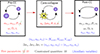Fig. 1. Graphic showing the connection between the free parameters and the constrained quantities in this study. The free parameters (shown in red) describe the pre-collapse orbit and the CC itself. The constrained quantities (shown in black) are either directly measured or are derived from auxiliary quantities (shown in blue), in which case they need to be treated carefully. The auxiliary post-CC system velocities vf are directly measured but unconstraining on their own. As a proxy for the inaccessible initial velocity components vi, we assume that these are consistent with (and can thus be drawn from) the measured velocity dispersion of the birth association Venv of the binary. The components of the net velocity vector Δv are constrained quantities. In the best-case observing scenario, we can obtain 10 distinct parameter constraints from the observations, but there are still 12 free parameters. If we further assume that the pre-collapse orbit was circular (which nullifies the true anomaly νi), we reduce the number of free parameters to 10, and the solution can be uniquely determined.

If we can further assume that the pre-collapse orbit was circular, e_i ≈ 0, then the true anomaly at the moment of collapse ν_i becomes irrelevant. More precisely, we constrain only the sum ω_i + ν_i, but not the individual terms. In this case, we reduce the number of free parameters to ten, and the problem has as many constraints as degrees of freedom.

In such circumstances, it is possible that the mapping between initial and final parameters is a bijection, in which case the free parameters could be estimated to arbitrarily high precision. We do not attempt to prove this, and in any event, finite measurement uncertainty is an unavoidable barrier to such arbitrarily high precision, particularly for the pre-CC velocities which are by necessity limited by the width of the dispersion in the birth association. Nevertheless, we demonstrate with our injection tests that, at least for the cases under consideration, when measurement uncertainties and the birth dispersion are taken to be very narrow, we can recover the injected values precisely.

2.5. Estimating the system and birth velocity distributions

To measure the three-dimensional velocity of a binary system, we make use of radial velocity, parallax, and proper motion measurements. Information on the natal kick cannot be inferred from the velocity of the system alone, we need to know the birth velocity of the binary to determine the change in the systemic velocity caused by the CC. Here, we describe the methodology of measuring the present day velocity and estimating the birth velocity, using VFTS 243 as an illustrative example. VFTS 243 is extragalactic and thus requires some care in deriving the transverse velocity solutions, as will also be the case for the systems in the BLOeM sample.

VFTS 243 was first identified in the VLT-FLAMES Tarantula survey (Evans et al. 2011; Sana et al. 2013) through large variations in the measured RV in different epochs. Further follow-up observations from the Tarantula Massive Binary Monitoring program (TMBM, PI: Sana, 090.D-0323 and 092.D-0136) allowed a characterization of its orbital parameters (Almeida et al. 2017); the RV of its barycenter was reported to be v_r,f = 261.50 ± 0.42 km s⁻¹.

For the tangential velocity components of VFTS 243, we make use of the results from the third Gaia data release (DR3, Gaia Collaboration 2023). Gaia reports correlated posterior solutions for the parallax and proper motion components for any given source. Unfortunately, since VFTS 243 is extragalactic, the reported parallax is negative, π = −0.047 ± 0.024 mas, which generally indicates that only a lower limit of ∼10 kpc can be obtained for the distance to the source (Lindegren et al. 2021). The distance to the LMC is d_LMC = 49.69 ± 0.63 kpc, measured independently with eclipsing binaries by Pietrzyński et al. (2019).

It is tempting to ignore the parallax solutions completely and directly combine the proper motion data with this independent distance measurement to derive the transverse velocity for VFTS 243. However, since the proper motion and parallax solutions are correlated to each other, samples in the posterior space with parallax values that are too low (high) compared to the true parallax are associated with proper motions that are proportionally too high (low). The reported proper motions, and thus the derived transverse velocities, therefore have a measurement uncertainty that is broadened by the inclusion of these extremal samples.

Instead, we performed an MCMC where the model parameters θ are the distance d_LMC and the two proper motions, μ_α and μ_δ. We used a normal distribution for the distance and broad uniform priors for the proper motions,

$$\begin{array}{cc}\hfill d_{\mathrm{LMC}}[\mathrm{kpc}]& \sim \mathcal{N}(49.69,0.63)\hfill \\ \hfill {\mu }_{\alpha }[\mathrm{mas}{\mathrm{yr}}^{-1}]& \sim U(-5,5)\hfill \\ \hfill {\mu }_{\delta }[\mathrm{mas}{\mathrm{yr}}^{-1}]& \sim U(-5,5).\hfill \end{array}$$

The likelihood on the measured parallax and proper motions is taken to be a multi-normal distribution,

$$\begin{array}{c}\hfill \mathcal{L}(\mathit{d}|\mathit{\theta })={\mathcal{N}}_3(\mathit{\theta },\mathbf{\Sigma }),\end{array}$$(4)

where d corresponds to the reported values of parallax and proper motions and Σ is the covariance matrix for these three quantities, provided by Gaia DR3. From the resulting posterior distributions, we calculate the tangential velocities of VFTS 243, v_α, f = 409.3 ± 9.6 km s⁻¹ and v_δ, f = 138.8 ± 7.6 km s⁻¹. In this way, we extract from the Gaia posteriors only the subset of samples which are consistent with the independently measured distance, and the resulting transverse velocity distributions are considerably more precise.

To estimate the birth velocity, we extend this same treatment to a larger sample. The prior on the birth velocity is the velocity dispersion of the host, V_env, which is assumed to be isotropic and normally distributed,

$$\begin{array}{c}\hfill {\mathit{v}}_{\mathrm{i}}\sim {\mathit{V}}_{\mathrm{env}}={\mathcal{N}}_3({\mathit{\mu }}_{\mathrm{env}},{\sigma }_{\mathrm{env}}^{2}I).\end{array}$$(5)

The velocity dispersion V_env is in turn calculated using a representative sample of systems within the Tarantula nebula with measured proper motions. We again perform an MCMC to excise the regions of the Gaia posteriors with parallax values that are inconsistent with the independently measured distance. Here, the model parameters are d_LMC, μ_env, σ_env and the velocities v_env,k of each system k in the representative sample. We use the same prior for d_LMC as above. For μ_env and σ_env we use broad uniform priors, while the prior for the velocities v_env,k follows from Eq. (5) with μ_env and σ_env as hyperparameters.

Some care is required in the choice of systems to include in the representative sample, as this may have a non-negligible impact on the resulting environment velocity distribution. For the radial velocity distribution, we choose only the SB2 binaries from the TMBM survey, reported by Almeida et al. (2017), as well as the ones reclassified from SB1 to SB2 using spectral disentangling by Shenar et al. (2022b). We do not include single stars or SB1 binaries, as these populations may be contaminated by systems that have previously been affected by their own natal kicks.

For the transverse velocities, we take the proper motion data for the same systems from Gaia DR3, but we take as additional quality cuts that the reported parallax is within 1-σ of the LMC parallax, that both proper motions have errors smaller than 0.1 mas yr⁻¹ and that the Renormalized Unit Weight Error (aka RUWE) of its fit is < 1.4. For each object in the sample, we consider a normal likelihood for the RV measurement, and for those that satisfy the quality cuts we include a likelihood on their parallax and proper motion as in Eq. (4). The total likelihood is determined as the product of all the individual likelihoods. Because of these additional quality cuts, the number of systems included in the transverse velocity distributions is smaller than that of the radial velocity distribution.

In Fig. 2, we show the distributions of the three systemic velocity components v_f of VFTS 243 in red. In blue, we show the inferred dispersion components V_env for its host, the Tarantula nebula. We can see that the velocity of VFTS 243 does not deviate significantly from the dispersion of its environment, which plays an important role in constraining its natal kick. There is a larger uncertainty in the distribution of tangential velocities of the environment, compared with the uncertainty in the RV distribution, owing to the smaller sample size, their broad spatial distribution, and the larger measurement errors compared to RVs.

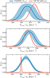Fig. 2. Velocity distributions for VFTS 243 and its host association. The measured velocity components for VFTS 243 (red), compared to the inferred dispersion of its birth association, the Tarantula nebula (blue, arbitrary scaling), estimated from the massive binaries in the TMBM survey. From top to bottom, the panels show the velocity in the direction of increasing RA and in the direction of increasing Dec and in the radial direction. For the Tarantula dispersion, a 90% credible interval of the inferred distributions is shown.

For the purpose of this work, we take the mean values of σ_env and of each component of μ_env, and use these to determine normal priors for each initial velocity component when inferring kicks,

$$\begin{array}{cc}\hfill v_{\alpha ,\mathrm{i}}[\mathrm{km}{\mathrm{s}}^{-1}]& \sim V_{\alpha ,\mathrm{env}}=\mathcal{N}(393,12)\hfill \\ \hfill v_{\delta ,\mathrm{i}}[\mathrm{km}{\mathrm{s}}^{-1}]& \sim V_{\delta ,\mathrm{env}}=\mathcal{N}(143,12)\hfill \\ \hfill v_{\mathrm{r},\mathrm{i}}[\mathrm{km}{\mathrm{s}}^{-1}]& \sim V_{\mathrm{r},\mathrm{env}}=\mathcal{N}(271,12).\hfill \end{array}$$

A potential future improvement is to treat μ_env and σ_env as hyperparameters, using as priors the posterior distributions that were inferred from the SB2 sample. The methods described here to determine the 3D velocity of VFTS 243 as well as the environment birth velocity distribution can be applied similarly to sources identified in the SMC in the BLOeM survey, using a corresponding parallax measurement (e.g., Graczyk et al. 2020).

We emphasize that the choice of systems is somewhat subjective and needs to be considered on a case-by-case basis. Indeed, VFTS 243 could have been born in NGC 2060, which has a slightly higher systemic radial velocity of about 277 km s⁻¹ (Sana et al. 2022). The SB2 population may also potentially be contaminated by dynamical runaways, artificially increasing the derived dispersion (Lennon et al. 2018; Stoop et al. 2024). In cases where the number of available SB2 systems is low, it may also be desirable to include single stars or SB1s despite the potential for contamination. Such considerations will be important in future analyses for constraining the birth velocities of inert BHBs.

3. Injection tests

In the ideal scenario, observations exist for an inert BHB that can constrain all the intrinsic and extrinsic parameters that describe its orbit, its orientation, and its velocity relative to birth. More commonly, some observations may not be available for a given binary, and only a subset of these data are known. Here, we use injection tests to explore how well we recover the parameters of interest as a function of the available observations and of assumptions about the environment and adopted prior distributions. We performed several injection analyses using two mock binaries: one which was circular pre-collapse (e_i = 0.0, discussed below) and the other moderately eccentric (e_i = 0.3, see Appendix B). The input parameters of both systems are described in Table 1.

We forward modeled the CC in these binaries (as described in Appendix A), then added to the calculated system velocity a birth velocity drawn randomly from a specified environment dispersion distribution. We assumed for convenience that the environment velocity distribution is described by a 3D Gaussian with mean μ_env = (100, 200, 50) km s⁻¹ (chosen for ease of validation), and a default dispersion σ_env = 1 km s⁻¹ in all directions. The dispersion is small for illustrative purposes, but we explore more realistic dispersion values in Sect. 3.2.

We injected typical measurement uncertainties into the post-CC properties and then performed the MCMC inference. The derived post-CC properties for both systems are shown in Table 2 along with the adopted measurement uncertainties.

3.1. Observational categories

We considered eight models, which are summarized in Table 3. The models {S, SV_R, SV_T, SV₃, SO, SOV_R, SOV_T, SOV₃ } are named according to the observational categories they include. The “S” indicates that the binary is observed spectroscopically as an SB1. All variations include spectroscopy, as this is required to infer m_1,f from stellar atmosphere modeling and thus break the degeneracy of the mass function. In principle, the inference could be done without stellar modeling using just the mass function. However, this would provide very weak constraints on the parameters of interest. The “O” is included when there is a resolved orbit from a close system with an astrometric binary solution. A “V_R”, “V_T”, or “V₃” is appended if the net system velocity change can be constrained in the radial direction Δv_r, both of the transverse directions Δv_α and Δv_δ, or all three, respectively (we do not consider cases where only one of the transverse velocity directions is constrained). These constraints are only included if a birth association has been identified and if the indicated components are measured in both the source and the host.

Figure 3a shows the resulting posteriors of the models that exclude the constraints from a resolved astrometric orbit, while Fig. 3b shows models that include these constraints. With more constraints, the posterior distributions tighten around the injected values, reducing the covered area by over an order of magnitude from the worst to best case (S to SOV₃). However, there are also some biases that appear when certain observations are omitted. We note, for example, model SOV_T in Fig. 3b. The 90% confidence interval (CI) correctly includes the true value in the 2D posterior, but the 1D distributions suggest greater support for a stronger natal kick and less mass loss. A systematic investigation into the cause of these biases is left to a future study.

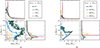Fig. 3. Impact of including different observations in a mock circular binary. Posteriors on the natal kick (vk) and mass loss (Δm2) are shown for when the various observational categories are included. Observational categories include spectroscopy (S), resolved astrometric orbit (O), and constraints on any of radial velocity (VR), transverse velocities (VT), or all three velocity components (V3). All categories include spectroscopy (see Sect. 3.1 for justification). Categories without (with) the astrometric orbit are shown on the left (right). Colors correspond to differences in the available velocity constraints: when there are no velocity constraints (S, SO: dark green), when only the RVs are constrained (SVR, SOVR: blue), when only the transverse velocities are constrained (SVT, SOVT: yellow), and when there are measurements in all three directions (SV3, SOV3: red). All results here apply for the circular mock system; the results for the eccentric mock system are shown in Fig. B.1. Black dashed lines show the true values. Contours capture the 90% confidence interval of the 2D distributions. (a) Initially circular binary, without a resolved orbit. (b) Initially circular binary, with a resolved orbit.

3.2. Impact of velocity dispersion in the birth cluster

In Fig. 4, we investigate the effect of velocity dispersion in the host association. In the default mock systems, we used a narrow velocity dispersion of 1 km s⁻¹ in all three directions to help illustrate the inference capabilities. Typical host clusters may have higher velocity dispersions, closer to 5 km s⁻¹ (Hénault-Brunet et al. 2012), while field OB stars may have velocity dispersions up to 10 km s⁻¹. (Carretero-Castrillo et al. 2023). We show the posteriors for Δm₂ and v_k when the dispersion is allowed to vary between 1, 3, and 10 km s⁻¹. In all cases, the circular mock system is used together with the circular prior, in the best-case observing scenario (SOV₃).

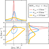Fig. 4. Inference variations due to the birth environment velocity dispersion. Posteriors on the natal kick vk and mass loss Δm2, when the birth environment has velocity dispersion in all three directions equal to 1, 3, or 10 km s−1 (red, blue, and yellow lines, respectively). The model shown here is for the initially circular mock system with the circular prior, in the best-case scenario SOV3. Black dashed lines show the true values.

As the dispersion increases, the injected values no longer lie within the 2D 90% CI. In particular, the inference finds more support for low kick magnitudes, which may not be surprising given that more of the post-CC velocity can be attributed to a larger velocity at birth. However, we caution against drawing deep conclusions from this single test and simply argue that biases may arise from the broadening of environment dispersions. As before, a deeper investigation into the precise nature of these biases is left to future work.

3.3. Impact of eccentricity

We explored the impact of pre-collapse eccentricity and the adopted eccentricity prior used in the inference. In Fig. 5, we show several corner plots for the parameters Δm₂ and v_k, using different eccentricity treatments. In all cases, we use the best-case observing scenario SOV₃ and the default velocity dispersion of 1 km s⁻¹.

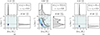Fig. 5. Role of eccentricity in a mock binary in the best-case observing scenario. Corner plots show Δm2 and vk posteriors in the best-case observing scenario (SOV3, see Sect. 3.1). In panel a, we correctly assume a circular prior for the initially circular mock system, whereas in panel b we used the eccentric prior for the initially circular system. In panel c, we use a circular prior for the initially eccentric mock system, to test the impact of prior misspecification. The gray shaded regions and quoted intervals indicate the 90% CI for the 1D distributions, while black contours indicate the 90% CI for the two parameter correlated distributions. Black, dashed lines show the true values. (a) Circular binary with circular prior. (b) Circular binary with eccentric prior. (c) Eccentric binary with circular prior.

In panel a, we assumed a circular prior for the initially circular mock system. In this case, the number of free parameters exactly matches the number of measured observables, and we recovered all the injected quantities with a high degree of precision, limited only by the measurement uncertainty.

In panel b we used the eccentric prior for the initially circular system. Here, the true value is within the 90% CI recovered by the inference for all parameters shown and is close to the primary peak in the posterior. However, the uncertainty intervals for the 1D distributions are roughly an order of magnitude larger than in panel a. Additionally, there is a prominent secondary peak, suggesting that the inference may find misleading solutions even when the priors contain all the true values. Notably, although the posterior support is broad, we can confidently rule out the low-v_k, low-Δm₂ region associated with direct collapse. In panel c, we assumed a circular prior for the initially eccentric system; this is a case of model misspecification. The recovered values are reported with high precision but far away from the true values.

The eccentricity prior therefore plays a particularly important role in the analysis. If the agnostic (eccentric) prior is used, we can rule out some parts of the parameter space to infer coarse attributes, such as whether the BH experienced direct collapse or not, but we cannot make precise statements about the true values of the inferred parameters. If the circular prior is used, we can determine tight constraints on the inferred parameters. However, these may be very incorrect if the pre-collapse system was not in fact circular.

4. VFTS 243

We demonstrate our inference pipeline on the LMC spectroscopic binary VFTS 243, which is one of the first widely accepted examples of a massive inert BHB system. Consisting of a ≈25 M_⊙ O-type star orbiting a ≳9 M_⊙ BH in a 10.4 d orbit, VFTS 243 is notable for its very low eccentricity, e = 0.017 ± 0.012 (Shenar et al. 2022a). The visible companion in VFTS 243 rotates super-synchronously, indicating that tidal synchronization has not occurred since BH formation. Since the tidal circularization timescale is shorter than the synchronization timescale, we therefore cannot attribute the low eccentricity to tidal effects (Shenar et al. 2022a). The orbital period, corresponding to a current separation of ∼36 R_⊙, is sufficiently short that the BH progenitor should have experienced mass transfer onto the companion. Altogether, the low eccentricity appears to be indicative of a weak natal kick and minimal mass loss during the CC event, from a progenitor that was at least partially stripped in a binary that circularized during a prior mass transfer event (Stevance et al. 2023; Klencki et al. 2022; Banagiri et al. 2023; Vigna-Gómez et al. 2024).

We focus on VFTS 243 as it represents a good test case of what will be possible with the BLOeM catalog in the SMC. As with the SMC binaries, VFTS 243 is too distant for astrometry to resolve the orbit. However, BLOeM data will produce spectroscopic constraints on many massive binaries in the SMC, providing source and host RVs, similarly to the VLT-FLAMES survey for the Tarantula nebula. And existing Gaia astrometric data combined with an independent distance measurement provides transverse velocities for sources in both Magellanic clouds. VFTS 243 and the upcoming BLOeM systems therefore fall into the observational category SV₃ introduced in Table 3. The spectroscopically obtained parameters reported for VFTS 243 in Shenar et al. (2022a) are reproduced in Table 4, together with the estimated systemic transverse and radial velocities from Gaia Collaboration (2023) and Almeida et al. (2017), respectively. For the environment velocity estimate, we follow the routine outlined in Sect. 2.5 (see Table 5).

4.1. Inference outcomes

The results of the inference for VFTS 243 are shown in Fig. 6, using the SV₃ model and assuming a circular orbit prior. We highlight only a few key parameters of interest, the BH progenitor mass m_2,i, the systemic velocity relative to the pre-collapse velocity Δ v, and the CC mass loss Δm₂ and natal kick v_k (posteriors for other parameters are shown in Appendix C). Even in the absence of a resolved orbit, the posteriors are informative and unimodal. As expected, the inference indicates that VFTS 243 formed with little mass loss and a weak natal kick.

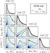Fig. 6. Best-case inference for VFTS 243. Here, we use the circular orbit prior with the SV3 model, which is the best case for an extra-Galactic system, combining spectroscopy as well as the full velocity vector of the system and the dispersion of its birth environment.

Variations on the inference of VFTS 243 due to different observations and priors. We compare the 1D posteriors of the mass loss Δm₂ and natal kick v_k, for VFTS 243. We include only models which do not require a resolved orbit (see Sect. 3.1). Models S, SV_R, SV_T, and SV₃ (solid lines) use the circular orbit prior, π(e_i) = δ(e_i). We additionally include the best-case observing model SV₃ with the full eccentricity prior, π(e_i) = U(0, 1) (black, dotted), identified as (SV₃).

For completeness, we also explore models S, SV_R, and SV_T to see the impact if we ignore some of the velocity components and to better compare to previous studies. In Fig. 7, we show the impact of these variations together with the best-case model SV₃ on the 1D posteriors for Δm₂ and v_k. These models all use the circular orbit prior. We additionally show model SV₃ using the agnostic eccentricity prior, as a check against model misspecification in case the pre-collapse orbit was not circular. All variations are consistent with low mass loss and small natal kicks, although the 90% credible intervals differ in some cases by a factor of four. This highlights the straightforward interpretation of circular inert BHBs which have not been affected by tides.

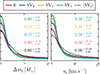Fig. 7. Variations on the inference of VFTS 243 due to different observations and priors. We compare the 1D posteriors of the mass loss Δm2 and natal kick vk, for VFTS 243. We include only models which do not require a resolved orbit (see Sect. 3.1). Models S, SVR, SVT, and SV3 (solid lines) use the circular orbit prior, π(e i)=δ(e i). We additionally include the best-case observing model SV3 with the full eccentricity prior, π(e i)=U(0, 1) (black, dotted), identified as (SV3).

4.2. Comparison to previous studies

Several recent studies also reported constraints on the natal kick and mass loss properties of VFTS 243 (Stevance et al. 2023; Banagiri et al. 2023; Vigna-Gómez et al. 2024). We qualitatively confirm the results in these previous studies that this system likely formed with a relatively small amount of mass loss and a modest natal kick that is consistent with 0, although there is some tension quantitatively with the results of Banagiri et al. (2023).

Stevance et al. (2023) used pre-computed models in the BPASS population synthesis code (Eldridge et al. 2008; Stanway & Eldridge 2018) to infer a natal kick v_k < 33 km s⁻¹ at 90% confidence. This is only marginally higher than the 26.5 km s⁻¹ upper limit reported here. Their best fit models also indicate mass loss Δm₂ ≈ 1 M_⊙, although this is not reported with an uncertainty interval. This value is slightly larger than, but consistent with, the median value reported here.

Banagiri et al. (2023) and Vigna-Gómez et al. (2024) both perform their inference directly on the observed properties of VFTS 243, with an agnostic treatment of the stellar and binary evolution history. Both include constraints on the RV for VFTS 243, but not the transverse velocity data. Thus, these studies are best compared to the SV_R curves.

Banagiri et al. (2023) report a 90% upper limit for the natal kick of either v_k < 72 km s⁻¹ or < 97 km s⁻¹, depending on the choice of prior, which is a factor of ∼3 − 4 larger than found here. They also report a 90% interval in the mass loss of either Δm₂/M_⊙ ∈ [0.4, 14.2] or [0.3, 14.4], again depending on the choice of prior, although elsewhere in the paper they claim a 90% lower mass loss constraint of either 0.69 M_⊙ or 0.77 M_⊙. These upper limits are also a factor of ∼3 − 4 higher than the upper limits reported here, and moreover our support at Δm₂ = 0 M_⊙ is in tension with their conclusions. However, this is not a direct one-to-one comparison, because Banagiri et al. (2023) do not account for the correlation between the RV constraint and the other parameters.

Meanwhile, Vigna-Gómez et al. (2024) report a natal kick which peaks at 0 km s⁻¹ with a 68% upper limit of 10 km s⁻¹ and an ejecta mass 68% upper limit of 1 M_⊙, also peaking at 0 M_⊙. To facilitate the direct comparison, we report here also our 68% confidence intervals on these parameters. At 68% confidence, we find the natal kick v_k ≤ 13.47 km s⁻¹ and the mass loss Δm₂ ≤ 1.34 M_⊙, both still peaking at 0, and only slightly larger than the values found in Vigna-Gómez et al. (2024). However, Vigna-Gómez et al. (2024) used top-hat likelihoods in place of Gaussians on all observed parameters, which is overly restrictive, in addition to using the RV measurement to inform the likelihood on the full systemic velocity. Thus, we consider the analysis framework here to be a more robust improvement over the previous methodology.

5. Discussion

5.1. Importance of the pre-collapse eccentricity prior

In our injection tests, we considered two systems, one which was circular pre-collapse and one which was eccentric. We also considered priors on the orbital eccentricity that were either circular, π(e_i) = δ(e_i), or were broad and uninformative, π(e_i) = U(0, 1). In the latter case, the posteriors become so broad that only coarse, qualitative statements can be made, even in the best-case observing scenario model SOV₃ (see Appendix B).

However, we cannot assume that all observed inert BHBs were circular prior to the CC. Some may not have interacted prior to CC, and so could have retained a natal eccentricity from the birth of the binary. Others may have been part of triple (or higher multiplicity) systems, as is expected for many massive stars (Moe & Di Stefano 2017). This would have a nontrivial effect on the orbits both pre- and post-CC, which we do not attempt to account for here. Additionally, even in the case of binaries which interacted prior to collapse, recent evidence suggests that mass transfer does not circularize binaries in all cases (e.g. Vigna-Gómez et al. 2020, and references therein), as has been the ubiquitous assumption in binary evolution models for many decades.

There is some observational evidence for eccentric, post-interaction binaries, particularly where one component is a WR star, such as the WR+O binary γ² Vel (aka WR 11) with a period P = 79 d and an eccentricity e ≈ 0.33 (Niemela & Sahade 1980; Eldridge 2009; Lamberts et al. 2017). Other such systems have eccentricities in the range e ∈ [0.1, 0.4], and periods between 3 and 5000 days, although the post-interaction nature has been debated for some of these (Marchenko et al. 1994; Schmutz & Koenigsberger 2019; Richardson et al. 2021, 2024; Holdsworth et al. 2024). Additionally, WR 140 is extremely eccentric, with e = 0.89, although it is in a wide, 7.93 yr orbit which again challenges the post-interaction hypothesis (Lau et al. 2022; Holdsworth et al. 2024). Recently, Pauli et al. (2022) reported the discovery of AzV 476, an O4+O9.5 binary in the SMC, with P = 9.4 d and e = 0.24. The authors argued that AzV 476 must be post-interaction based on the similarity in component masses, which is in tension with the large difference in luminosities.

Moreover, recent theoretical work has argued for eccentricity retention during mass transfer in long period, roughly equal mass binaries (Rocha et al. 2025), as well as eccentricity pumping due to phase dependent Roche-lobe overflow (Sepinsky et al. 2007, 2009, 2010) or in post-mass transfer binaries due to the presence of a circumbinary disk (Vos et al. 2015; Valli et al. 2024). Given this, we might expect the true population of pre-collapse binaries to be circularized due to mass transfer up to a limiting period, above which systems can retain more eccentricity (Rocha et al. 2025). In general, we suggest caution when considering the role of pre-collapse eccentricity on the inference results from SIDEKICKS.JL.

5.2. Ideal candidates for observation

As the population of inert BHBs grows, determining which systems might provide useful constraints on BH formation will become crucial. A critical assumption to the inference here is that the binary orbit has not changed substantially since formation of the BH. Close binaries that have experienced mass transfer after CC, or which have circularized under the influence of tidal interactions, modify key elements of the orbit and thus invalidate this assumption (e.g., Hut 1981). Similarly, binaries that have traveled significantly through their galactic environments may have systemic velocities that have been modified, or potentially experienced perturbative flyby interactions from a third body (Stegmann et al. 2024). This is unlikely to be the case for binaries with an O/B-type primary, which provide an upper age limit of at most ∼10 Myr. However, it may be problematic for binaries with low-mass primaries, such as the three Gaia BHs.

The BLOeM survey (Shenar et al. 2024) is expected to yield precisely the kinds of systems that can provide tight constraints on BH formation, with largely the same caveats as VFTS 243. Gaia DR4 is also expected to provide solutions to many more massive binaries, including potentially hundreds of O/B+BH binary candidates, many of which should be useful for this type of inference (Janssens et al. 2022). Such systems would require spectroscopic follow-up to confirm the BH companion, such as from the Sloan Digital Sky Survey (Almeida et al. 2023). Those for which the orbit can be resolved may provide tighter constraints on the BH formation than inert BHBs from the more distant BLOeM sample. However, they may also be biased toward longer periods, where the assumption of pre-collapse circularity might not hold. Crucially, BHs observed in any kind of binary are necessarily biased toward low, nondisruptive kicks so that even with a large population of inert BHBs analyzed with SIDEKICKS.JL, we will not be able to truly probe the full BH natal kick landscape.

While not the focus of this study, inert NS-binaries can also be used with this inference pipeline, assuming the same conditions as described above for BHs. This would provide valuable constraints on the weak end of the NS natal kick distribution, which is important in the formation of NS-XRBs, binary NSs, short gamma-ray bursts, kilonovae, and other related phenomena, and complements the well-studied constraints on the stronger end of the NS natal kick distribution. Notably, the lower masses of NSs compared to BHs make it more challenging to distinguish NSs from low mass nondegenerate stars when interpreting the companions in SB1 binaries.

5.3. Model dependency of the primary mass

A strength of our methodology is the lack of model dependent quantities involved. The priors are mostly chosen to be broad and noninformative, the CC mechanism is treated agnostically, and the effect of the CC on the binary is a straightforward adaptation of the 2-body problem. However, as noted in Sect. 2.2, we cannot determine the component masses in a model-independent way; we are limited by the degeneracies of the mass function.

Primary mass estimates must come from some other model dependent technique, such as the spectroscopic mass derived from the surface gravity and radius, or the evolutionary mass approximated from matching the position of the star in the HR-diagram to precomputed single star evolution tracks (see Shenar et al. 2022a). The evolutionary mass in particular may be unreliable, especially given that many of the inert BHBs are expected to have interacted prior to the formation of the BH, in which case the structure and interpretation of the primary star may be biased (Renzo et al. 2023). These systematic uncertainties propagate through the inference, and may complicate efforts to estimate CC and pre-collapse parameters.

5.4. Extensions to the analysis

The inference pipeline described in this study could be extended in a number of ways, to incorporate other types of binaries or observations than those studied here. High-mass XRBs, such as Cyg X-1, typically circularize due to tidal forces, modifying their periods and eccentricities from their values following CC. However, the tidal circularization mechanism conserves angular momentum. Thus, by treating the circularization period,

$$\begin{array}{c}\hfill P_{\mathrm{circ}}=P_{\mathrm{f}}{(1-e_{\mathrm{f}}^2)}^{3/2},\end{array}$$(6)

of the binary as an observable, instead of the period and eccentricity independently, we could perform a similar inference on the high-mass XRB population, assuming tidal forces are the dominating perturbation in the post-CC evolution of the binary. For Cyg X-1 in particular, recent observations that resulted in a ∼50% increase in the estimated BH mass (Miller-Jones et al. 2021) warrant an updated investigation of the natal kick constraints, which we plan to address in an upcoming publication.

Additionally, eclipsing binaries may experience self-lensing and brighten during the eclipse, providing a tight constraint on the inclination of the binary, and possibly also an independent estimate on the BH mass if the parallax and companion effective temperature are also constrained (Masuda & Hotokezaka 2019; Chawla et al. 2024). Moreover, inert BHBs may be identifiable via ellipsoidal variability or relativistic beaming, constraining functions of the masses, inclination, and semi-major axis (Chawla et al. 2024). Furthermore, Mahy et al. (2022) showed that for spectroscopic binaries, a large measured v sin i constrains the inclination angle to be below a given threshold to prevent the luminous star from spinning above critical rotation. If the CC was not a direct collapse, then the orbital angular momentum vector may well have rotated during the explosion. Thus this becomes a constraint only on the maximum pre-collapse inclination i_i.

Although not the focus of this study, the current pipeline can also be used to constrain the natal kick angles and thereby to study variations from an isotropic kick distribution. For the case of VFTS 243 (see Appendix C), we indeed observe a modest preference for polar kicks, although the kick magnitude is so low for this system that such a preference is not significant. Valli et al. (2025) recently argued that preferentially polar natal kicks are required to explain the observed period-eccentricity distribution of Be XRBs.

5.5. Impact on the primary

Key quantities that we ignored throughout include those related to the impact of a SN explosion on the primary star, both in the form of a mass differential Δm₁ (due to ablation or accretion) or an impact velocity injection v_imp (Wheeler et al. 1975; Pfahl et al. 2002; Liu et al. 2015; Hirai et al. 2018; Ogata et al. 2021). These may be negligible in all but the closest binary systems, though such effects could potentially be observable in late time SN follow-up observations (Hirai & Podsiadlowski 2022). If included, these would increase the size of the parameter space and broaden the posteriors on the parameters of interest.

6. Summary and conclusions

Black hole natal kicks persist as an astrophysical uncertainty with broad consequences across different fields, including impacts on (among others) BH X-ray binaries; BHs in globular clusters; free-floating BHs, which could contribute to microlensing observations and dark matter estimates (Cirelli et al. 2024); and binary BHs and BH-NSs, which may be detectable as gravitational-wave sources. In this work, we have presented a Bayesian inference and MCMC sampling package, SIDEKICKS.JL, that uses a broad collection of observables for inert BHBs to constrain BH natal kicks and mass loss as well as the pre-collapse orbital parameters that provide useful constraints on binary evolution models. While previous works have studied the impact of a core-collapse event in a binary with an eccentric orbit (Pfahl et al. 2002; Hurley et al. 2002), we have expanded on these efforts by tracking all the Keplerian orbital elements of the binary together with the post-collapse velocity vector.

We argue that the inclusion of these extra observables provides critical constraints on the parameters of core-collapse that have been missed in previous analyses, which only account for the post-CC speed. In the special case where the binary was circular prior to BH formation and the current orbit can be completely characterized, we demonstrated that all the collapse and pre-collapse parameters, particularly the natal kick and mass loss, can be recovered precisely. We further explored the consequences of excluding some of these observed parameters, either through a lack of observational data or physical unattainability, as well as incorrectly assuming that the pre-collapse orbit was circular.

Finally, we have demonstrated the inference capabilities of SIDEKICKS.JL by inferring the properties of VFTS 243, an inert BHB in the LMC. We highlighted the improvements of our method with respect to previous studies that did not correctly treat all the orientation and velocity elements. We report a mass loss of $\mathrm{\Delta }{m}_2=0.{07}_{-0.07}^{+2.82}{M}_{\odot }$ and a natal kick of $v_{\text{k}}=0.{00}_{-0.00}^{+26.45}$ km s⁻¹, which is qualitatively in agreement with the previous literature values for this system.

A particular strength of the method presented in this work is that it is almost completely independent of uncertain astrophysical models, such as the details of the core-collapse mechanism and dependence on the progenitor structure, although it does depend on uncertain mass estimates for the visible star from either spectroscopic mass estimates or evolutionary models. This analysis can be readily applied to any wide binary containing a massive star and a compact object, including NSs, with negligible tidal interactions. Such binaries are expected to be observed in large numbers with the BLOeM spectroscopic survey as well as with the upcoming Gaia DR4 release.

Data availability

All data, as well as the inference, analysis, and plotting scripts required to reproduce the results and figures in this paper, are stored at https://doi.org/10.5281/zenodo.15267344

Acknowledgments

We thank the anonymous referee for their useful suggestions which improved the manuscript. Data analysis was performed with a custom inference package, SIDEKICKS.JL. SIDEKICKS.JL made extensive use of the Bayesian inference library TURING.JL (Ge et al. 2018) and the plotting package MAKIE.JL (Danisch & Krumbiegel 2021), all of which are written in the JULIA language (Bezanson et al. 2017). This work has made use of data from the European Space Agency (ESA) mission Gaia (https://www.cosmos.esa.int/gaia), processed by the Gaia Data Processing and Analysis Consortium (DPAC, https://www.cosmos.esa.int/web/gaia/dpac/consortium). Funding for the DPAC has been provided by national institutions, in particular the institutions participating in the Gaia Multilateral Agreement. RW acknowledges support from the KU Leuven Research Council through grant iBOF/21/084. PM acknowledges support from the FWO senior fellowship number 12ZY523N and the European Research Council (ERC) under the European Union’s Horizon 2020 research and innovation program (grant agreement 101165213/Star-Grasp). HS and KD acknowledge the financial support from the Flemish Government under the long-term structural Methusalem grant METH/24/012 at KU Leuven. ME acknowledges funding from the FWO research grants G099720N and G0B3823N. LM acknowledges the Belgian Science Policy Office (BELSPO) for the financial support. SJ acknowledges support from International postdoctoral research fellowships of the Japan Society for the Promotion of Science (JSPS). LRP acknowledges support by grants PID2019-105552RB-C41 and PID2022-137779OB-C41 and PID2022-140483NB-C22 funded by MCIN/AEI/10.13039/501100011033 by “ERDF A way of making Europe”. DP acknowledges financial support from the FWO in the form of a junior postdoctoral fellowship grant number No. 1256225N. AACS is supported by the Deutsche Forschungsgemeinschaft (DFG – German Research Foundation) in the form of an Emmy Noether Research Group – Project-ID 445674056 (SA4064/1-1, PI Sander). TS acknowledges support from the Israel Science Foundation (ISF) under grant number 0603225041 and from the European Research Council (ERC) under the European Union’s Horizon 2020 research and innovation program (grant agreement 101164755/METAL).

References

Appendix A: Post explosion orbital elements of an eccentric binary

A.1. Pre-explosion properties

We considered a binary system composed of two masses, m_1,i and m_2,i, with a semi-major axis a_i and an eccentricity e_i. We consider the case where star 2 undergoes an explosion at a point in the orbit with a true anomaly ν_i. We refer to properties right before and right after the explosion with subindices “i" and “f", respectively. We define a coordinate frame oriented such that ${\widehat{e}}_{\text{y}}$ is a unit vector pointing from star 2 toward its companion at the moment of explosion. The unit vector ${\widehat{e}}_{\text{z}}$ points in the direction of the orbital angular momentum and as usual ${\widehat{e}}_{\text{x}}={\widehat{e}}_{\text{y}}\times {\widehat{e}}_{\text{z}}$ (see Fig. A.1). We can then define the position vectors of both stars as a function of arbitrary true anomaly ν as

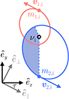Fig. A.1. Definitions of unit axes used to determine the post-explosion parameters of an eccentric binary. Shown is the binary at the moment of explosion of star 2 with a true anomaly νi. The black circle indicates the center of mass of the system. The unit axes ${\widehat{e}}_{\text{x}}$ and ${\widehat{e}}_{\text{y}}$ are defined in terms of the line joining both stars at the moment of explosion, while the unit axes ${\widehat{e}}_{\Vert }$ and ${\widehat{e}}_{\perp }$ are defined in terms of the direction of motion of star 2 at the moment of explosion. These sets of unit vectors are related by a rotation with an angle τ.

$$\begin{array}{c}\hfill \begin{array}{cc}\hfill {\mathit{r}}_1& =r_1[-sin(\nu -{\nu }_{\mathrm{i}}){\widehat{e}}_{\mathrm{x}}+cos(\nu -{\nu }_{\mathrm{i}}){\widehat{e}}_{\mathrm{y}}]\hfill \\ \hfill {\mathit{r}}_2& =r_2[sin(\nu -{\nu }_{\mathrm{i}}){\widehat{e}}_{\mathrm{x}}-cos(\nu -{\nu }_{\mathrm{i}}){\widehat{e}}_{\mathrm{y}}].\hfill \end{array}\end{array}$$(A.1)

The distance of each star to the center of mass is given by

$$\begin{array}{c}\hfill r_1=a_{\mathrm{i}}\frac{m_{2,\mathrm{i}}}{M_{\mathrm{i}}}f(\nu ,e_{\mathrm{i}}),r_2=a_{\mathrm{i}}\frac{m_{1,\mathrm{i}}}{M_{\mathrm{i}}}f(\nu ,e_{\mathrm{i}}),\end{array}$$(A.2)

where M_i = m_1,i + m_2,i is the total mass of the pre-explosion system. The quantity f(ν, e_i) determines the instantaneous separation a_if(ν, e_i) of the binary,

$$\begin{array}{c}\hfill f(\nu ,e_{\mathrm{i}})=\frac{1-e_{\mathrm{i}}^2}{1+e_{\mathrm{i}}cos\nu }.\end{array}$$(A.3)

The time derivative of the true anomaly can be derived from Kepler’s second and third law, resulting in

$$\begin{array}{c}\hfill \dot{\nu }=\sqrt{\frac{G{M}_{\mathrm{i}}}{a_{\mathrm{i}}^3}}\frac{{(1+e_{\mathrm{i}}cos\nu )}^2}{{(1-e_{\mathrm{i}}^2)}^{3/2}}.\end{array}$$(A.4)

Combining these results, we can write the individual velocities of each component with respect to the center of mass of the binary, at the moment of explosion (ν = ν_i),

$$\begin{array}{c}\hfill \begin{array}{cc}\hfill {\mathit{v}}_{1,\mathrm{i}}& =-\frac{m_{2,\mathrm{i}}}{M_{\mathrm{i}}}\sqrt{\frac{G{M}_{\mathrm{i}}}{a_{\mathrm{i}}(1-e_{\mathrm{i}}^2)}}[(1+e_{\mathrm{i}}cos{\nu }_{\mathrm{i}}){\widehat{e}}_{\mathrm{x}}-e_{\mathrm{i}}sin{\nu }_{\mathrm{i}}{\widehat{e}}_{\mathrm{y}}],\hfill \\ \hfill {\mathit{v}}_{2,\mathrm{i}}& =\frac{m_{1,\mathrm{i}}}{M_{\mathrm{i}}}\sqrt{\frac{G{M}_{\mathrm{i}}}{a_{\mathrm{i}}(1-e_{\mathrm{i}}^2)}}[(1+e_{\mathrm{i}}cos{\nu }_{\mathrm{i}}){\widehat{e}}_{\mathrm{x}}-e_{\mathrm{i}}sin{\nu }_{\mathrm{i}}{\widehat{e}}_{\mathrm{y}}].\hfill \end{array}\end{array}$$(A.5)

We can then define a new set of unit vectors in terms of the instantaneous velocity of the exploding star. The unit vector pointing in the direction of v_2,i is

$$\begin{array}{c}\hfill {\widehat{e}}_{\Vert }=\frac{1}{\sqrt{1+2e_{\mathrm{i}}cos{\nu }_{\mathrm{i}}+e_{\mathrm{i}}^2}}[(1+e_{\mathrm{i}}cos{\nu }_{\mathrm{i}}){\widehat{e}}_{\mathrm{x}}-e_{\mathrm{i}}sin{\nu }_{\mathrm{i}}{\widehat{e}}_{\mathrm{y}}].\end{array}$$(A.6)

The individual velocities can then be expressed as

$$\begin{array}{c}\hfill {\mathit{v}}_{1,\mathrm{i}}=-v_{\mathrm{rel},\mathrm{i}}\frac{m_{2,\mathrm{i}}}{M_{\mathrm{i}}}{\widehat{e}}_{\Vert },{\mathit{v}}_{2,\mathrm{i}}=v_{\mathrm{rel},\mathrm{i}}\frac{m_{1,\mathrm{i}}}{M_{\mathrm{i}}}{\widehat{e}}_{\Vert },\end{array}$$(A.7)

where the relative velocity between the stars is given by

$$\begin{array}{c}\hfill v_{\mathrm{rel},\mathrm{i}}=|{\mathit{v}}_{1,\mathrm{i}}-{\mathit{v}}_{2,\mathrm{i}}|=g({\nu }_{\mathrm{i}},e_{\mathrm{i}})\sqrt{\frac{G{M}_{\mathrm{i}}}{a_{\mathrm{i}}}}.\end{array}$$(A.8)

The function g(ν_i, e_i) represents the deviation from the relative velocity of a circular orbit and is given by

$$\begin{array}{c}\hfill g({\nu }_{\mathrm{i}},e_{\mathrm{i}})=\sqrt{\frac{1+2e_{\mathrm{i}}cos{\nu }_{\mathrm{i}}+e_{\mathrm{i}}^2}{1-e_{\mathrm{i}}^2}}.\end{array}$$(A.9)

It is also useful to define a unit vector perpendicular to ${\widehat{e}}_{\Vert }$,

$$\begin{array}{c}\hfill {\widehat{e}}_{\perp }=\frac{1}{\sqrt{1+2e_{\mathrm{i}}cos{\nu }_{\mathrm{i}}+e_{\mathrm{i}}^2}}[e_{\mathrm{i}}sin{\nu }_{\mathrm{i}}{\widehat{e}}_{\mathrm{x}}+(1+e_{\mathrm{i}}cos{\nu }_{\mathrm{i}}){\widehat{e}}_{\mathrm{y}}],\end{array}$$(A.10)

which satisfies ${\widehat{e}}_{\Vert }\times {\widehat{e}}_{\perp }={\widehat{e}}_{\text{z}}$. The different unit vectors are then related via

$$\begin{array}{c}\hfill \begin{array}{c}\hfill {\widehat{e}}_{\mathrm{x}}=j({\nu }_{\mathrm{i}},e_{\mathrm{i}}){\widehat{e}}_{\Vert }-h({\nu }_{\mathrm{i}},e_{\mathrm{i}}){\widehat{e}}_{\perp },\\ \hfill {\widehat{e}}_{\mathrm{y}}=h({\nu }_{\mathrm{i}},e_{\mathrm{i}}){\widehat{e}}_{\Vert }+j({\nu }_{\mathrm{i}},e_{\mathrm{i}}){\widehat{e}}_{\perp },\end{array}\end{array}$$(A.11)

where the functions h(ν_i, e_i) and j(ν_i, e_i) satisfy that h(ν_i, e_i)² + j(ν_i, e_i)² = 1 and are defined as

$$\begin{array}{c}\hfill \begin{array}{c}\hfill h({\nu }_{\mathrm{i}},e_{\mathrm{i}})=\frac{-e_{\mathrm{i}}sin{\nu }_{\mathrm{i}}}{\sqrt{1+2e_{\mathrm{i}}cos{\nu }_{\mathrm{i}}+e_{\mathrm{i}}^2}},\\ \hfill j({\nu }_{\mathrm{i}},e_{\mathrm{i}})=\frac{1+e_{\mathrm{i}}cos{\nu }_{\mathrm{i}}}{\sqrt{1+2e_{\mathrm{i}}cos{\nu }_{\mathrm{i}}+e_{\mathrm{i}}^2}}.\end{array}\end{array}$$(A.12)

In terms of h(ν_i, e_i) and j(ν_i, e_i) we have that the angle τ, measured counter-clockwise from ${\widehat{e}}_{\Vert }$ to ${\widehat{e}}_{\mathrm{x}}$ (see Fig. A.1), satisfies that sin τ = −h(ν_i, e_i) and cos τ = j(ν_i, e_i).

For simplicity, we define

$$\begin{array}{c}\hfill f_{\nu ,\mathrm{i}}\equiv f({\nu }_{\mathrm{i}},e_{\mathrm{i}}),f_{\nu ,\mathrm{f}}\equiv f({\nu }_{\mathrm{f}},e_{\mathrm{f}}),\end{array}$$(A.13)

as well as

$$\begin{array}{c}\hfill g_{\nu ,\mathrm{i}}\equiv g({\nu }_{\mathrm{i}},e_{\mathrm{i}}),h_{\nu ,\mathrm{i}}\equiv h({\nu }_{\mathrm{i}},e_{\mathrm{i}}),j_{\nu ,\mathrm{i}}\equiv j({\nu }_{\mathrm{i}},e_{\mathrm{i}}).\end{array}$$(A.14)

A.2. Post-explosion semi-major axis

We considered that star 2 undergoes a SN, which removes mass leaving a remnant of mass m_2,f while imparting on it a velocity kick v_k. The direction of the kick is defined in terms of a polar angle θ and an azimuthal angle ϕ, setting the kick direction with respect to ${\widehat{e}}_{\Vert }$, ${\widehat{e}}_{\perp }$ and ${\widehat{e}}_{\text{z}}$ (see Figure A.2):

$$\begin{array}{c}\hfill {\mathit{v}}_{\mathrm{k}}=v_{\mathrm{k}}{\widehat{v}}_{\mathrm{k}},{\widehat{v}}_{\mathrm{k}}=cos\theta {\widehat{e}}_{\Vert }+sin\theta cos\varphi {\widehat{e}}_{\perp }+sin\theta sin\varphi {\widehat{e}}_{\mathrm{z}}.\end{array}$$(A.15)

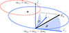Fig. A.2. Illustration of the natal kick. The angles θ and ϕ define the direction of the kick velocity vk with respect to the unit vectors ${\widehat{e}}_{\Vert }$, ${\widehat{e}}_{\perp }$ and ${\widehat{e}}_{\text{z}}$.

For full generality, we also considered the possibility that the CC event removes part of the mass of star 1, leaving a final mass m_1,f while imparting an impact velocity in the ${\widehat{e}}_{\text{y}}$ direction of magnitude v_imp, leaving a system with a final mass M_f = m_1,f + m_2,f. The final velocities of each component are then

$$\begin{array}{c}\hfill {\mathit{v}}_{1,\mathrm{f}}={\mathit{v}}_{1,\mathrm{i}}+v_{\mathrm{imp}}{\widehat{e}}_{\mathrm{y}},{\mathit{v}}_{2,\mathrm{f}}={\mathit{v}}_{2,\mathrm{i}}+{\mathit{v}}_{\mathrm{k}}.\end{array}$$(A.16)

The final semi-major axis a_f can be determined from the total orbital energy in the frame of the new center of mass,

$$\begin{array}{c}\hfill E_{\mathrm{f}}=-\frac{G{M}_{\mathrm{f}}}{2a_{\mathrm{f}}},\end{array}$$(A.17)

which can be computed from the separation and velocities post-explosion (with respect to the new center of mass). The center of mass velocity post-explosion is given by

$$\begin{array}{c}\hfill {\mathit{v}}_{\mathrm{CM},\mathrm{f}}=\frac{m_{1,\mathrm{f}}{\mathit{v}}_{1,\mathrm{f}}+m_{2,\mathrm{f}}{\mathit{v}}_{2,\mathrm{f}}}{M_{\mathrm{f}}},\end{array}$$(A.18)

from which the individual velocities in the reference frame of the new center of mass are

$$\begin{array}{c}\hfill \begin{array}{c}\hfill {\mathit{v}}_{\mathrm{CM},1,\mathrm{f}}={\mathit{v}}_{1,\mathrm{f}}-{\mathit{v}}_{\mathrm{CM},\mathrm{f}}=\frac{m_{2,\mathrm{f}}}{M_{\mathrm{f}}}({\mathit{v}}_{1,\mathrm{f}}-{\mathit{v}}_{2,\mathrm{f}}),\\ \hfill {\mathit{v}}_{\mathrm{CM},2,\mathrm{f}}={\mathit{v}}_{2,\mathrm{f}}-{\mathit{v}}_{\mathrm{CM},\mathrm{f}}=\frac{m_{1,\mathrm{f}}}{M_{\mathrm{f}}}({\mathit{v}}_{2,\mathrm{f}}-{\mathit{v}}_{1,\mathrm{f}}).\end{array}\end{array}$$(A.19)

The final orbital energy can then be computed by considering the instantaneous orbital separation remains fixed,

$$\begin{array}{c}\hfill E_{\mathrm{f}}=-\frac{G{m}_{1,\mathrm{f}}{m}_{2,\mathrm{f}}}{a_{\mathrm{i}}{f}_{\nu ,\mathrm{i}}}+\frac{m_{1,\mathrm{f}}{m}_{2,\mathrm{f}}}{2M_{\mathrm{f}}}{({\mathit{v}}_{2,\mathrm{f}}-{\mathit{v}}_{1,\mathrm{f}})}^2,\end{array}$$(A.20)

where to compute the kinetic energy term it is convenient to write

$$\begin{array}{c}\hfill {\mathit{v}}_{2,\mathrm{f}}-{\mathit{v}}_{1,\mathrm{f}}=v_{\mathrm{rel},\mathrm{i}}({\widehat{e}}_{\Vert }-\beta {\widehat{e}}_{\mathrm{y}}+\alpha {\widehat{v}}_{\mathrm{k}}),\beta \equiv \frac{v_{\mathrm{imp}}}{v_{\mathrm{rel},\mathrm{i}}},\alpha \equiv \frac{v_{\mathrm{k}}}{v_{\mathrm{rel},\mathrm{i}}}.\end{array}$$(A.21)

Expanding ${\widehat{e}}_{\text{y}}$ and ${\widehat{v}}_{\text{k}}$ in terms of ${\widehat{e}}_{\Vert }$, ${\widehat{e}}_{\perp }$ and ${\widehat{e}}_{\text{z}}$, it is straightforward to show that

$$\begin{array}{c}\hfill \begin{array}{c}\hfill \frac{{({\mathit{v}}_{2,\mathrm{f}}-{\mathit{v}}_{1,\mathrm{f}})}^2}{v_{\mathrm{rel},\mathrm{i}}^2}=1+{\alpha }^2+{\beta }^2+2[\alpha cos\theta -h_{\nu ,\mathrm{i}}\beta (1+\alpha cos\theta )\\ \hfill -j_{\nu ,\mathrm{i}}\beta \alpha sin\theta cos\varphi ].\end{array}\end{array}$$(A.22)

Combining Equations (A.8) and (A.20) we can express the total energy as

$$\begin{array}{c}\hfill E_{\mathrm{f}}=-\frac{G{m}_{1,\mathrm{f}}{m}_{2,\mathrm{f}}}{f_{\nu ,\mathrm{i}}{a}_{\mathrm{i}}}(1-\frac{\xi }{2}),\end{array}$$(A.23)

where

$$\begin{array}{c}\hfill \xi \equiv f_{\nu ,\mathrm{i}}{g}_{\nu ,\mathrm{i}}^2\frac{M_{\mathrm{i}}}{M_{\mathrm{f}}}\frac{{({\mathit{v}}_{2,\mathrm{f}}-{\mathit{v}}_{1,\mathrm{f}})}^2}{v_{\mathrm{rel},\mathrm{i}}^2}.\end{array}$$(A.24)

This also implies that the orbit becomes unbound if ξ > 2. Equating the last expression to the final orbital energy given in Equation (A.17) we obtain the post-explosion semi-major axis:

$$\begin{array}{c}\hfill a_{\mathrm{f}}=\frac{f_{\nu ,\mathrm{i}}{a}_{\mathrm{i}}}{2-\xi }.\end{array}$$(A.25)

A.3. Post-explosion eccentricity

Similar to the derivation of the post-explosion semi-major axis, the post-explosion eccentricity can be computed in terms of the final orbital angular momentum,

$$\begin{array}{c}\hfill L_{\mathrm{f}}=m_{1,\mathrm{f}}{m}_{2,\mathrm{f}}\sqrt{\frac{G{a}_{\mathrm{f}}(1-e_{\mathrm{f}}^2)}{M_{\mathrm{f}}}}.\end{array}$$(A.26)

The orbital angular momentum in the new center of mass frame is also given by

$$\begin{array}{c}\hfill {\mathit{L}}_{\mathrm{f}}=m_{1,\mathrm{f}}{\mathit{r}}_{\mathrm{CM},1,\mathrm{f}}\times {\mathit{v}}_{\mathrm{CM},1,\mathrm{f}}+m_{2,\mathrm{f}}{\mathit{r}}_{\mathrm{CM},2,\mathrm{f}}\times {\mathit{v}}_{\mathrm{CM},2,\mathrm{f}},\end{array}$$(A.27)

where r_CM,1,f and r_CM,2,f are vectors pointing from the new center of mass to each component,

$$\begin{array}{c}\hfill {\mathit{r}}_{\mathrm{CM},1,\mathrm{f}}=f_{\nu ,\mathrm{i}}{a}_{\mathrm{i}}\frac{m_{2,\mathrm{f}}}{M_{\mathrm{f}}}{\widehat{e}}_{\mathrm{y}},{\mathit{r}}_{\mathrm{CM},2,\mathrm{f}}=-f_{\nu ,\mathrm{i}}{a}_{\mathrm{i}}\frac{m_{1,\mathrm{f}}}{M_{\mathrm{f}}}{\widehat{e}}_{\mathrm{y}}.\end{array}$$(A.28)

Combining the previous two Equations together with Equations (A.19) and (A.21) we find that

$$\begin{array}{c}\hfill {\mathit{L}}_{\mathrm{f}}=-f_{\nu ,\mathrm{i}}{a}_{\mathrm{i}}\frac{m_{1,\mathrm{f}}{m}_{2,\mathrm{f}}}{M_{\mathrm{f}}}{v}_{\mathrm{rel},\mathrm{i}}[{\widehat{e}}_{\mathrm{y}}\times ({\widehat{e}}_{\Vert }+\alpha {\widehat{v}}_{\mathrm{k}})].\end{array}$$(A.29)

The magnitude of the vector in brackets is straightforward to determine by expressing it in terms of ${\widehat{e}}_{\Vert }$, ${\widehat{e}}_{\perp }$ and ${\widehat{e}}_{\text{z}}$, resulting in

$$\begin{array}{c}\hfill \begin{array}{cc}\hfill {[{\widehat{e}}_{\mathrm{y}}\times ({\widehat{e}}_{\Vert }+\alpha {\widehat{v}}_{\mathrm{k}})]}^2& ={\alpha }^2{sin}^2\theta {sin}^2\varphi +[h_{\nu ,\mathrm{i}}\alpha sin\theta cos\varphi \hfill \\ \hfill & -j_{\nu ,\mathrm{i}}{(1+\alpha cos\theta )]}^2.\hfill \end{array}\end{array}$$(A.30)

Combing Equations (A.29) and (A.8) we find that

$$\begin{array}{c}\hfill L_{\mathrm{f}}^2=f_{\nu ,\mathrm{i}}{a}_{\mathrm{i}}G\frac{{(m_{1,\mathrm{f}}{m}_{2,\mathrm{f}})}^2}{M_{\mathrm{f}}}\eta .\end{array}$$(A.31)

where

$$\begin{array}{c}\hfill \eta \equiv f_{\nu ,\mathrm{i}}{g}_{\nu ,\mathrm{i}}^2\frac{M_{\mathrm{i}}}{M_{\mathrm{f}}}{[{\widehat{e}}_{\mathrm{y}}\times ({\widehat{e}}_{\Vert }+\alpha {\widehat{v}}_{\mathrm{k}})]}^2.\end{array}$$(A.32)

Combining Equations (A.25), (A.26) and (A.31) we obtain the post-explosion orbital eccentricity:

$$\begin{array}{c}\hfill e_{\mathrm{f}}=\sqrt{1+(\xi -2)\eta }.\end{array}$$(A.33)

A.4. Center of mass velocity

The velocity of the center of mass can be determined from Equation (A.18), but it can also be determined in a straightforward way by accounting for the change in momentum of the binary components. If we write the center of mass velocity as

$$\begin{array}{c}\hfill {\mathit{v}}_{\mathrm{CM},\mathrm{f}}=v_{\mathrm{CM},\Vert }{\widehat{e}}_{\Vert }+v_{\mathrm{CM},\perp }{\widehat{e}}_{\perp }+v_{\mathrm{CM},\mathrm{z}}{\widehat{e}}_{\mathrm{z}},\end{array}$$(A.34)

then the individual components of the velocity are given by

$$\begin{array}{c}\hfill \begin{array}{cc}\hfill v_{\mathrm{CM},\Vert }& =\frac{1}{M_{\mathrm{f}}}[\frac{v_{\mathrm{rel},\mathrm{i}}}{M_{\mathrm{i}}}(m_{1,\mathrm{i}}{m}_{2,\mathrm{f}}-m_{1,\mathrm{f}}{m}_{2,\mathrm{i}})\hfill \\ \hfill & m_{2,\mathrm{f}}{v}_{\mathrm{k}}cos\theta +h_{\nu ,\mathrm{i}}{m}_{1,\mathrm{f}}{v}_{\mathrm{imp}}],\hfill \\ \hfill v_{\mathrm{CM},\perp }& =\frac{1}{M_{\mathrm{f}}}(m_{2,\mathrm{f}}{v}_{\mathrm{k}}sin\theta cos\varphi +j_{\nu ,\mathrm{i}}{m}_{1,\mathrm{f}}{v}_{\mathrm{imp}}),\hfill \\ \hfill v_{\mathrm{CM},\mathrm{z}}& =\frac{m_{2,\mathrm{f}}{v}_{\mathrm{k}}sin\theta sin\varphi }{M_{\mathrm{f}}}.\hfill \end{array}\end{array}$$(A.35)

We note that this is the final velocity of the center of mass of the binary in a reference frame where the binary was static prior to the explosion, while for comparison to an observed system we need to account for any pre-collapse velocity.

A.5. Observer frame of reference

We also need to account for the relationship between the direction of motion of the system and the Keplerian elements, including the inclination i, the longitude of the ascending node Ω, and the argument of periastron ω of the companion. We take the convention here that the ascending node corresponds to the intersection point of the orbit with the celestial plane at which the star is moving away from the observer. We derive the expected properties that would be visible from a reference frame centered on the observer, with unit vectors pointing in the directions of celestial north $\widehat{N}$, celestial west $\widehat{W}$, and toward the observer $\widehat{O}$ (these then satisfy $\widehat{W}\times \widehat{N}=\widehat{O}$). This basis is identical (up to reflection) of the δ − α − r basis used above for the velocity components, but is used here to make it easier to visualize the rotations.

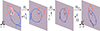Fig. A.3. Series of rotations to convert from the frame of reference of the binary to that of the observer. The binary frame of reference is spanned by the unit vectors ${\widehat{e}}_{\Vert }$, ${\widehat{e}}_{\perp }$ and ${\widehat{e}}_{\text{z}}$, while the observer frame of reference is defined by $\widehat{N}$, $\widehat{W}$, and $\widehat{O}$. The left-most figure shows the pre-explosion system, including the position of the ascending node for m1 and the descending node for m2, indicated with pluses. The following panels apply the rotation matrices Rϵ, Ri and RΩ. For reference, a transparent plane is shown that remains fixed during rotations, with its edges aligned with ${\widehat{e}}_{\Vert }$ and ${\widehat{e}}_{\perp }$ at the leftmost panel (darker shading indicates the orbit is behind the plane).

If we consider a vector

$$\begin{array}{c}\hfill \mathit{b}=b_{\Vert }{\widehat{e}}_{\Vert }+b_{\perp }{\widehat{e}}_{\perp }+b_z{\widehat{e}}_{\mathrm{z}}=b_{\mathrm{W}}\widehat{W}+b_{\mathrm{N}}\widehat{N}+b_{\mathrm{O}}\widehat{O},\end{array}$$(A.36)

then the components of b in the observer frame can be determined by a series of rotations,

$$\begin{array}{c}\hfill \left(\begin{array}{c}{b}_{\mathrm{W}}\\ b_{\mathrm{N}}\\ b_{\mathrm{O}}\end{array}\right)=R_{\mathrm{\Omega }}{R}_i{R}_{ϵ}\left(\begin{array}{c}{b}_{\Vert }\\ b_{\perp }\\ b_z\end{array}\right).\end{array}$$(A.37)

The rotation matrix R_ϵ is meant to put the ascending node of star 1 in the direction (0, 1, 0), and is given by

$$\begin{array}{c}\hfill R_{ϵ}=\left(\begin{array}{ccc}cosϵ& -sinϵ& 0\\ sinϵ& cosϵ& 0\\ 0& 0& 1\end{array}\right).\end{array}$$(A.38)

where ϵ = ω + ν − τ,

$$\begin{array}{c}\hfill \tau =\{\begin{array}{cc}arccos{j}_{\nu }\hfill & 0\le \nu <\pi \hfill \\ -arccos{j}_{\nu }\hfill & \pi \le \nu <2\pi \hfill \end{array}.\end{array}$$(A.39)

The following rotation matrix, R_i, corrects for the inclination and sets the direction (0, 0, 1) to point toward the observer:

$$\begin{array}{c}\hfill R_i=\left(\begin{array}{ccc}cosi& 0& -sini\\ 0& 1& 0\\ sini& 0& cosi\end{array}\right).\end{array}$$(A.40)

We emphasize that the inclination here is defined on the range [0, π], to account for all inclinations in which the star is moving away from the observer at the ascending node.

Finally, the rotation R_Ω rotates the projected orbit in the plane of the sky by Ω so that the direction (0, 1, 0) points toward the ascending node,

$$\begin{array}{c}\hfill R_{\mathrm{\Omega }}=\left(\begin{array}{ccc}cos\mathrm{\Omega }& -sin\mathrm{\Omega }& 0\\ sin\mathrm{\Omega }& cos\mathrm{\Omega }& 0\\ 0& 0& 1\end{array}\right).\end{array}$$(A.41)

We note that we have omitted time-dependent subscripts here as the rotation can be applied to both the pre- and post-collapse binary. The center of mass velocity of the binary in the observer frame can then be obtained by applying Equation (A.37) to the components of v_CM,f.

A.6. Post-explosion inclination

To determine the inclination of the resulting binary, we need to compute the angle between the orbital angular momentum post-explosion and the unit vector $\widehat{O}$. Starting from Equation A.29 we have that the unit vector pointing in the direction of the final orbital angular momentum is

$$\begin{array}{c}\hfill {\widehat{L}}_{\mathrm{f}}=\frac{-{\widehat{e}}_{\mathrm{y}}\times ({\widehat{e}}_{\Vert }+\alpha {\widehat{v}}_{\mathrm{k}})}{|{\widehat{e}}_{\mathrm{y}}\times ({\widehat{e}}_{\Vert }+\alpha {\widehat{v}}_{\mathrm{k}})|},\end{array}$$(A.42)

which has components

$$\begin{array}{c}\hfill \begin{array}{cc}\hfill {\widehat{L}}_{\mathrm{f}}·{\widehat{e}}_{\Vert }& =-\frac{j_{\nu ,\mathrm{i}}\alpha sin\theta sin\varphi }{|{\widehat{e}}_{\mathrm{y}}\times ({\widehat{e}}_{\Vert }+\alpha {\widehat{v}}_{\mathrm{k}})|}\hfill \\ \hfill {\widehat{L}}_{\mathrm{f}}·{\widehat{e}}_{\perp }& =\frac{h_{\nu ,\mathrm{i}}\alpha sin\theta sin\varphi }{|{\widehat{e}}_{\mathrm{y}}\times ({\widehat{e}}_{\Vert }+\alpha {\widehat{v}}_{\mathrm{k}})|}\hfill \\ \hfill {\widehat{L}}_{\mathrm{f}}·{\widehat{e}}_{\mathrm{z}}& =-\frac{h_{\nu ,\mathrm{i}}\alpha sin\theta cos\varphi -j_{\nu ,\mathrm{i}}(1+\alpha cos\theta )}{|{\widehat{e}}_{\mathrm{y}}\times ({\widehat{e}}_{\Vert }+\alpha {\widehat{v}}_{\mathrm{k}})|},\hfill \end{array}\end{array}$$(A.43)

with the denominator given by Equation (A.30). The full components of the angular momentum in the base given by $\widehat{W}$, $\widehat{N}$ and $\widehat{O}$ can then be derived using Equation (A.37). With the component of ${\widehat{L}}_{\text{f}}$ that points in the $\widehat{O}$ direction we can directly extract the post-explosion inclination:

$$\begin{array}{c}\hfill i_{\mathrm{f}}=arccos({\widehat{L}}_{\mathrm{f}}·\widehat{O})\end{array}$$(A.44)

A.7. Post-explosion longitude of the ascending node

The longitude of the ascending node is the angle, measured counterclockwise on the plane of the sky, between the direction $\widehat{N}$ and the vector pointing from the center of mass toward the ascending node. Such a unit vector can be taken by the cross product between ${\widehat{L}}_{\text{f}}$ and $\widehat{O}$, both of which are perpendicular to the vector pointing toward the ascending node. Calling this unit vector ${\widehat{\mathrm{\Omega }}}_{\text{f}}$ and noting that the ascending node is the one where the object is moving away from the observer, we have that (see Figure A.4)

$$\begin{array}{c}\hfill {\widehat{\mathrm{\Omega }}}_{\mathrm{f}}=\frac{{\widehat{L}}_{\mathrm{f}}\times \widehat{O}}{|{\widehat{L}}_{\mathrm{f}}\times \widehat{O}|}.\end{array}$$(A.45)

The longitude of the ascending node can then be computed as

$$\begin{array}{c}\hfill {\mathrm{\Omega }}_{\mathrm{f}}=\{\begin{array}{cc}arccos({\widehat{\mathrm{\Omega }}}_{\mathrm{f}}·\widehat{N})\hfill & {\widehat{\mathrm{\Omega }}}_{\mathrm{f}}·\widehat{W}\le 0\hfill \\ 2\pi -arccos({\widehat{\mathrm{\Omega }}}_{\mathrm{f}}·\widehat{N})\hfill & {\widehat{\mathrm{\Omega }}}_{\mathrm{f}}·\widehat{W}>0\hfill \end{array}.\end{array}$$(A.46)

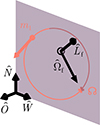Fig. A.4. Orientation of the orbital angular momentum in the observer reference frame. The orbital angular momentum vector ${\widehat{L}}_{\text{f}}$ and a vector pointing from the center of mass of the binary to the ascending node ${\widehat{\mathrm{\Omega }}}_{\text{f}}$ orient the post-explosion orbit of the visible star. Both ${\widehat{L}}_{\text{f}}$ and $\widehat{O}$ are perpendicular to ${\widehat{\mathrm{\Omega }}}_{\text{f}}$, but are not perpendicular to each other. In the particular case shown here ${\widehat{\mathrm{\Omega }}}_{\text{f}}·\widehat{W}>0$, such that ${\mathrm{\Omega }}_{\text{f}}=2\pi -arccos({\widehat{\mathrm{\Omega }}}_{\text{f}}·\widehat{N})$.

A.8. Post-explosion true anomaly

We next calculate the true anomaly ν_f immediately after the explosion, which we used to calculate the post-explosion argument of periastron ω_f. The distance between the binary components is the same right before and right after the explosion, such that (see Equation A.3):

$$\begin{array}{c}\hfill f_{\nu ,\mathrm{i}}{a}_{\mathrm{i}}=f_{\nu ,\mathrm{f}}{a}_{\mathrm{f}}.\end{array}$$(A.47)

The cosine of the final true anomaly is then

$$\begin{array}{c}\hfill cos{\nu }_{\mathrm{f}}=\frac{1}{e_{\mathrm{f}}}[\frac{a_{\mathrm{f}}(1-e_{\mathrm{f}}^2)}{f_{\nu ,\mathrm{i}}{a}_{\mathrm{i}}}-1].\end{array}$$(A.48)

The actual value then depends on whether we are moving away (0 ≤ ν_f < π) or toward (π ≤ ν_f < 2π) periastron. This can be determined with the ${\widehat{e}}_{\text{y}}$ component of v_CM,1,f, as this is still the axis connecting the two components. From Equation (A.35) we have that

$$\begin{array}{c}\hfill {\mathit{v}}_{\mathrm{CM},1,\mathrm{f}}·{\widehat{e}}_{\mathrm{y}}=v_{\mathrm{imp}}-h_{\nu ,\mathrm{i}}(\frac{m_{2,\mathrm{i}}}{M_{\mathrm{i}}}{v}_{\mathrm{rel},\mathrm{i}}+v_{\mathrm{CM},\Vert })-j_{\nu ,\mathrm{i}}{v}_{\mathrm{CM},\perp }.\end{array}$$(A.49)

Using this, the true anomaly post-explosion is given by:

$$\begin{array}{c}\hfill {\nu }_{\mathrm{f}}=\{\begin{array}{cc}{\displaystyle arccos\left\{\frac{1}{e_{\mathrm{f}}}[\frac{a_{\mathrm{f}}(1-e_{\mathrm{f}}^2)}{f_{\nu ,\mathrm{i}}{a}_{\mathrm{i}}}-1]\right\}}\hfill & {\mathit{v}}_{\mathrm{CM},1,\mathrm{f}}·{\widehat{e}}_{\mathrm{y}}>0\hfill \\ {\displaystyle 2\pi -arccos\left\{\frac{1}{e_{\mathrm{f}}}[\frac{a_{\mathrm{f}}(1-e_{\mathrm{f}}^2)}{f_{\nu ,\mathrm{i}}{a}_{\mathrm{i}}}-1]\right\}}\hfill & {\mathit{v}}_{\mathrm{CM},1,\mathrm{f}}·{\widehat{e}}_{\mathrm{y}}<0\hfill \end{array}.\end{array}$$(A.50)

Fig. A.5. Illustration of the different special cases to compute the argument of periastron for the post-explosion orbit of the visible star. See Equation A.52 for reference. The black arrow shows the vector $\widehat{y}$ while the gray arrow shows ${\widehat{\mathrm{\Omega }}}_{\text{f}}$, which point from the center of mass to the visible star and the ascending node respectively.

A.9. Post-explosion argument of periastron

Given that we know a unit vector pointing from the center of mass to star 1, and a unit vector pointing toward the ascending node, we can determine the angle between these two vectors,

$$\begin{array}{c}\hfill \lambda =arccos(\widehat{y}·{\widehat{\mathrm{\Omega }}}_{\mathrm{f}}).\end{array}$$(A.51)

In order to determine the argument of periastron after explosion ω_f, we need to combine ν_f and λ in a smart way, depending on the relative location between star 1 and the ascending node in the post-explosion orbit. The full set of conditions is as follows,

$$\begin{array}{c}\hfill {\omega }_{\mathrm{f}}=\{\begin{array}{cc}\lambda -{\nu }_{\mathrm{f}}\hfill & ({\widehat{e}}_{\mathrm{y}}\times {\widehat{\mathrm{\Omega }}}_{\mathrm{f}})·{\widehat{L}}_{\mathrm{f}}\le 0\wedge \lambda >{\nu }_{\mathrm{f}}\hfill \\ 2\pi +\lambda -{\nu }_{\mathrm{f}}\hfill & ({\widehat{e}}_{\mathrm{y}}\times {\widehat{\mathrm{\Omega }}}_{\mathrm{f}})·{\widehat{L}}_{\mathrm{f}}\le 0\wedge \lambda \le {\nu }_{\mathrm{f}}\hfill \\ 2\pi -\lambda -{\nu }_{\mathrm{f}}\hfill & ({\widehat{e}}_{\mathrm{y}}\times {\widehat{\mathrm{\Omega }}}_{\mathrm{f}})·{\widehat{L}}_{\mathrm{f}}>0\wedge \lambda +{\nu }_{\mathrm{f}}\le 2\pi \hfill \\ 4\pi -\lambda -{\nu }_{\mathrm{f}}\hfill & ({\widehat{e}}_{\mathrm{y}}\times {\widehat{\mathrm{\Omega }}}_{\mathrm{f}})·{\widehat{L}}_{\mathrm{f}}>0\wedge \lambda +{\nu }_{\mathrm{f}}>2\pi \hfill \end{array}.\end{array}$$(A.52)

Each of these cases is illustrated in Figure A.5.

Appendix B: Injection analysis for the eccentric system

In Fig. B.1, we provide the full corner plot that results from the injection analyses binary, while varying which observations are included. The plot is the same as Fig. 3 except this one is for the initially eccentric mock system. All posteriors are substantially broader than in the case of the circular mock binary. However, for all the models with any velocity constraints (namely, all except S and SO), we can still rule out the 0 km s⁻¹ natal kick - 0 M_⊙ corner associated with direct collapse SNe at the 90% confidence level.

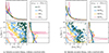Fig. B.1. Impact of including different observations in a mock eccentric binary. Posteriors on the natal kick (vk) and mass loss (Δm2), when the various observational categories are included. Observational categories include spectroscopy (S), resolved astrometric orbit (O), and constraints on any of radial velocity (VR), transverse velocities (VT), or all three velocity components (V3). All categories include spectroscopy (see Sec. 3.1 for justification). Categories without (with) the astrometric orbit are shown on the left (right). Colors correspond to differences in the available velocity constraints: when there are no velocity constraints (e.g., due to no host association; S, SO: dark green), when there are measured RVs for the source and host (SVR, SOVR: blue), when there are measured transverse velocities for the source and host (SVT, SOVT: yellow), and when there are measured velocities in all three directions for the source and host (SV3, SOV3: red). All results here apply for the eccentric mock system; the results for the circular mock system are shown in Fig. 3. Black dashed lines show the true values. Contours capture the 90% confidence interval of the 2D distributions.

Appendix C: Full corner plots for VFTS 243

In Figs. C.1 and C.2, we show the corner plots for the VFTS 243 analysis, for a broader set of the parameters of interest. Both plots use the best-case observing scenario SV₃; In Fig. C.1, we used the circular prior π(e_i) = δ(e_i), and in Fig. C.2, we used the eccentric prior π(e_i) = U(0, 1).

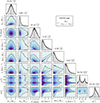Fig. C.1. Corner plot for VFTS 243, using the circular prior. Posteriors shown here include the initial masses and orbital period, the post-SN system velocity relative to the birth velocity, and the parameters that describe the SN mass loss and natal kick. The observing model is SV3, which is the best case available for this system given that it is too far to resolve the orbit.

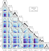Fig. C.2. Corner plot for VFTS 243, using the eccentric prior. Posteriors shown here include the initial masses, orbital period, and eccentricity, the post-SN system velocity relative to the birth velocity, and the parameters that describe the SN mass loss and natal kick. The observing model is SV3, which is the best case available for this system given that it is too far to resolve the orbit.

All Tables

References

- Almeida, L. A., Sana, H., Taylor, W., et al. 2017, A&A, 598, A84 [NASA ADS] [CrossRef] [EDP Sciences] [Google Scholar]
- Almeida, A., Anderson, S. F., Argudo-Fernández, M., et al. 2023, ApJS, 267, 44 [NASA ADS] [CrossRef] [Google Scholar]
- Andrews, J. J., & Kalogera, V. 2022, ApJ, 930, 159 [NASA ADS] [CrossRef] [Google Scholar]
- Antonini, F., & Gieles, M. 2020, MNRAS, 492, 2936 [CrossRef] [Google Scholar]
- Arzoumanian, Z., Chernoff, D. F., & Cordes, J. M. 2002, ApJ, 568, 289 [NASA ADS] [CrossRef] [Google Scholar]
- Atri, P., Miller-Jones, J. C. A., Bahramian, A., et al. 2019, MNRAS, 489, 3116 [NASA ADS] [CrossRef] [Google Scholar]
- Banagiri, S., Doctor, Z., Kalogera, V., Kimball, C., & Andrews, J. J. 2023, ApJ, 959, 106 [NASA ADS] [CrossRef] [Google Scholar]
- Banyard, G., Mahy, L., Sana, H., et al. 2023, A&A, 674, A60 [NASA ADS] [CrossRef] [EDP Sciences] [Google Scholar]
- Baumgardt, H., & Hilker, M. 2018, MNRAS, 478, 1520 [Google Scholar]
- Baumgardt, H., He, C., Sweet, S. M., et al. 2019, MNRAS, 488, 5340 [CrossRef] [Google Scholar]
- Bezanson, J., Edelman, A., Karpinski, S., & Shah, V. B. 2017, SIAM Rev., 59, 65 [Google Scholar]
- Blaauw, A. 1961, Bull. Astron. Inst. Netherlands, 15, 265 [NASA ADS] [Google Scholar]
- Boersma, J. 1961, Bull. Astron. Inst. Netherlands, 15, 291 [NASA ADS] [Google Scholar]
- Brandt, N., & Podsiadlowski, P. 1995, MNRAS, 274, 461 [NASA ADS] [CrossRef] [Google Scholar]
- Breivik, K., Chatterjee, S., & Larson, S. L. 2017, ApJ, 850, L13 [CrossRef] [Google Scholar]
- Brisken, W. F., Fruchter, A. S., Goss, W. M., Herrnstein, R. M., & Thorsett, S. E. 2003, AJ, 126, 3090 [NASA ADS] [CrossRef] [Google Scholar]
- Broekgaarden, F. S., Berger, E., Stevenson, S., et al. 2022, MNRAS, 516, 5737 [NASA ADS] [CrossRef] [Google Scholar]
- Burdge, K. B., El-Badry, K., Kara, E., et al. 2024, Nature, 635, 316 [NASA ADS] [CrossRef] [Google Scholar]
- Burrows, A., Wang, T., Vartanyan, D., & Coleman, M. S. B. 2023, ArXiv e-prints [arXiv:2311.12109] [Google Scholar]
- Burrows, A., Wang, T., & Vartanyan, D. 2024, ApJ, 964, L16 [NASA ADS] [CrossRef] [Google Scholar]
- Callister, T. A., Farr, W. M., & Renzo, M. 2021, ApJ, 920, 157 [NASA ADS] [CrossRef] [Google Scholar]
- Carretero-Castrillo, M., Ribó, M., & Paredes, J. M. 2023, A&A, 679, A109 [NASA ADS] [CrossRef] [EDP Sciences] [Google Scholar]
- Chakrabarti, S., Simon, J. D., Craig, P. A., et al. 2023, AJ, 166, 6 [NASA ADS] [CrossRef] [Google Scholar]
- Chan, C., Müller, B., & Heger, A. 2020, MNRAS, 495, 3751 [NASA ADS] [CrossRef] [Google Scholar]
- Chawla, C., Chatterjee, S., Shah, N., & Breivik, K. 2024, ApJ, 975, 163 [NASA ADS] [Google Scholar]
- Cirelli, M., Strumia, A., & Zupan, J. 2024, ArXiv e-prints [arXiv:2406.01705] [Google Scholar]
- Coleman, M. S. B., & Burrows, A. 2022, MNRAS, 517, 3938 [NASA ADS] [CrossRef] [Google Scholar]
- Danisch, S., & Krumbiegel, J. 2021, JOSS, 6, 3349 [Google Scholar]
- Dashwood Brown, C., Gandhi, P., & Zhao, Y. 2024, MNRAS, 527, L82 [Google Scholar]
- Dickson, N., Smith, P. J., Hénault-Brunet, V., Gieles, M., & Baumgardt, H. 2024, MNRAS, 529, 331 [NASA ADS] [CrossRef] [Google Scholar]
- Dray, L. M., Dale, J. E., Beer, M. E., King, A. R., & Napiwotzki, R. 2006, Ap&SS, 304, 279 [Google Scholar]
- El-Badry, K., Rix, H.-W., Quataert, E., et al. 2023a, MNRAS, 518, 1057 [Google Scholar]
- El-Badry, K., Rix, H.-W., Cendes, Y., et al. 2023b, MNRAS, 521, 4323 [NASA ADS] [CrossRef] [Google Scholar]
- Eldridge, J. J. 2009, MNRAS, 400, L20 [NASA ADS] [CrossRef] [Google Scholar]
- Eldridge, J. J., Izzard, R. G., & Tout, C. A. 2008, MNRAS, 384, 1109 [Google Scholar]
- Evans, C. J., Taylor, W. D., Hénault-Brunet, V., et al. 2011, A&A, 530, A108 [NASA ADS] [CrossRef] [EDP Sciences] [Google Scholar]
- Fortin, F., García, F., Chaty, S., Chassande-Mottin, E., & Simaz Bunzel, A. 2022, A&A, 665, A31 [NASA ADS] [CrossRef] [EDP Sciences] [Google Scholar]
- Gaia Collaboration (Vallenari, A., et al.) 2023, A&A, 674, A1 [NASA ADS] [CrossRef] [EDP Sciences] [Google Scholar]
- Gaia Collaboration (Panuzzo, P., et al.) 2024, A&A, 686, L2 [NASA ADS] [CrossRef] [EDP Sciences] [Google Scholar]
- Ge, H., Xu, K., & Ghahramani, Z. 2018, Proceedings of the Twenty-first International Conference on Artificial Intelligence and Statistics (PMLR), 1682 [Google Scholar]
- Giesers, B., Dreizler, S., Husser, T.-O., et al. 2018, MNRAS, 475, L15 [NASA ADS] [CrossRef] [Google Scholar]
- Giesers, B., Kamann, S., Dreizler, S., et al. 2019, A&A, 632, A3 [NASA ADS] [CrossRef] [EDP Sciences] [Google Scholar]
- Graczyk, D., Pietrzyński, G., Thompson, I. B., et al. 2020, ApJ, 904, 13 [Google Scholar]
- Hénault-Brunet, V., Evans, C. J., Sana, H., et al. 2012, A&A, 546, A73 [CrossRef] [EDP Sciences] [Google Scholar]
- Hills, J. G. 1983, ApJ, 267, 322 [NASA ADS] [CrossRef] [Google Scholar]
- Hirai, R., & Mandel, I. 2021, PASA, 38, e056 [NASA ADS] [CrossRef] [Google Scholar]
- Hirai, R., & Podsiadlowski, P. 2022, MNRAS, 517, 4544 [Google Scholar]
- Hirai, R., Podsiadlowski, P., & Yamada, S. 2018, ApJ, 864, 119 [NASA ADS] [CrossRef] [Google Scholar]
- Hobbs, G., Lorimer, D. R., Lyne, A. G., & Kramer, M. 2005, MNRAS, 360, 974 [Google Scholar]
- Holdsworth, A., Richardson, N., Schaefer, G. H., et al. 2024, ApJ, 977, 185 [Google Scholar]
- Homan, M. D., & Gelman, A. 2014, J. Mach. Learn. Res., 15, 1593 [Google Scholar]
- Hurley, J. R., Tout, C. A., & Pols, O. R. 2002, MNRAS, 329, 897 [Google Scholar]
- Hut, P. 1981, A&A, 99, 126 [NASA ADS] [Google Scholar]
- Igoshev, A. P., Chruslinska, M., Dorozsmai, A., & Toonen, S. 2021, MNRAS, 508, 3345 [NASA ADS] [CrossRef] [Google Scholar]
- Janka, H.-T., & Kresse, D. 2024, Ap&SS, 369, 80 [NASA ADS] [CrossRef] [Google Scholar]
- Janka, H.-T., Melson, T., & Summa, A. 2016, Annu. Rev. Nucl. Part. Sci., 66, 341 [Google Scholar]
- Janka, H.-T., Wongwathanarat, A., & Kramer, M. 2022, ApJ, 926, 9 [NASA ADS] [CrossRef] [Google Scholar]
- Janssens, S., Shenar, T., Sana, H., et al. 2022, A&A, 658, A129 [NASA ADS] [CrossRef] [EDP Sciences] [Google Scholar]
- Janssens, S., Shenar, T., Sana, H., & Marchant, P. 2023, A&A, 670, A79 [NASA ADS] [CrossRef] [EDP Sciences] [Google Scholar]
- Kalogera, V. 1996, ApJ, 471, 352 [Google Scholar]
- Karpov, S. V., & Lipunov, V. M. 2001, Astron. Lett., 27, 645 [Google Scholar]
- Katz, J. I. 1975, Nature, 253, 698 [NASA ADS] [CrossRef] [Google Scholar]
- Kimball, C., Imperato, S., Kalogera, V., et al. 2023, ApJ, 952, L34 [Google Scholar]
- Klencki, J., Istrate, A., Nelemans, G., & Pols, O. 2022, A&A, 662, A56 [NASA ADS] [CrossRef] [EDP Sciences] [Google Scholar]
- Koshimoto, N., Kawanaka, N., & Tsuna, D. 2024, ApJ, 973, 5 [Google Scholar]
- Lam, C. Y., Lu, J. R., Udalski, A., et al. 2022, ApJ, 933, L23 [NASA ADS] [CrossRef] [Google Scholar]
- Lamberts, A., Millour, F., Liermann, A., et al. 2017, MNRAS, 468, 2655 [NASA ADS] [CrossRef] [Google Scholar]
- Lau, R. M., Hankins, M. J., Han, Y., et al. 2022, Nat. Astron., 6, 1308 [NASA ADS] [CrossRef] [Google Scholar]
- Lennon, D. J., Evans, C. J., van der Marel, R. P., et al. 2018, A&A, 619, A78 [NASA ADS] [CrossRef] [EDP Sciences] [Google Scholar]
- Lindegren, L., Bastian, U., Biermann, M., et al. 2021, A&A, 649, A4 [EDP Sciences] [Google Scholar]
- Liu, Z.-W., Tauris, T. M., Röpke, F. K., et al. 2015, A&A, 584, A11 [NASA ADS] [CrossRef] [EDP Sciences] [Google Scholar]
- Mahy, L., Sana, H., Shenar, T., et al. 2022, A&A, 664, A159 [NASA ADS] [CrossRef] [EDP Sciences] [Google Scholar]
- Mandel, I. 2016, MNRAS, 456, 578 [Google Scholar]
- Marchenko, S. V., Moffat, A. F. J., & Koenigsberger, G. 1994, ApJ, 422, 810 [NASA ADS] [CrossRef] [Google Scholar]
- Mashian, N., & Loeb, A. 2017, MNRAS, 470, 2611 [NASA ADS] [CrossRef] [Google Scholar]
- Masuda, K., & Hotokezaka, K. 2019, ApJ, 883, 169 [NASA ADS] [CrossRef] [Google Scholar]
- Mezzacappa, A. 2023, IAU Symp., 362, 215 [Google Scholar]
- Miller-Jones, J. C. A., Bahramian, A., Orosz, J. A., et al. 2021, Science, 371, 1046 [Google Scholar]
- Mirabel, I. F., & Rodrigues, I. 2003, Science, 300, 1119 [Google Scholar]
- Moe, M., & Di Stefano, R. 2017, ApJS, 230, 15 [Google Scholar]
- Mróz, P., Udalski, A., & Gould, A. 2022, ApJ, 937, L24 [CrossRef] [Google Scholar]
- Müller, B. 2020, Liv. Rev. Comput. Astrophys., 6, 3 [Google Scholar]
- Nagarajan, P., & El-Badry, K. 2025, PASP, 137, 34203 [Google Scholar]
- Niemela, V. S., & Sahade, J. 1980, ApJ, 238, 244 [Google Scholar]
- O’Doherty, T. N., Bahramian, A., Miller-Jones, J. C. A., et al. 2023, MNRAS, 521, 2504 [CrossRef] [Google Scholar]
- Offner, S. S. R., Moe, M., Kratter, K. M., et al. 2023, ASP Conf. Ser., 534, 275 [NASA ADS] [Google Scholar]
- Ogata, M., Hirai, R., & Hijikawa, K. 2021, MNRAS, 505, 2485 [NASA ADS] [CrossRef] [Google Scholar]
- Pauli, D., Oskinova, L. M., Hamann, W. R., et al. 2022, A&A, 659, A9 [NASA ADS] [CrossRef] [EDP Sciences] [Google Scholar]
- Pfahl, E., Rappaport, S., & Podsiadlowski, P. 2002, ApJ, 573, 283 [NASA ADS] [CrossRef] [Google Scholar]
- Pietrzyński, G., Graczyk, D., Gallenne, A., et al. 2019, Nature, 567, 200 [Google Scholar]
- Podsiadlowski, P., Pfahl, E., & Rappaport, S. 2005, ASP Conf. Ser., 328, 327 [Google Scholar]
- Rastello, S., Iorio, G., Mapelli, M., et al. 2023, MNRAS, 526, 740 [NASA ADS] [CrossRef] [Google Scholar]
- Renzo, M., Zapartas, E., de Mink, S. E., et al. 2019, A&A, 624, A66 [NASA ADS] [CrossRef] [EDP Sciences] [Google Scholar]
- Renzo, M., Zapartas, E., Justham, S., et al. 2023, ApJ, 942, L32 [NASA ADS] [CrossRef] [Google Scholar]
- Repetto, S., Davies, M. B., & Sigurdsson, S. 2012, MNRAS, 425, 2799 [Google Scholar]
- Richardson, N. D., Lee, L., Schaefer, G., et al. 2021, ApJ, 908, L3 [NASA ADS] [CrossRef] [Google Scholar]
- Richardson, N. D., Schaefer, G. H., Eldridge, J. J., et al. 2024, ApJ, 977, 78 [Google Scholar]
- Rocha, K. A., Hur, R., Kalogera, V., et al. 2025, ApJ, 983, 39 [Google Scholar]
- Sahu, K. C., Anderson, J., Casertano, S., et al. 2022, ApJ, 933, 83 [Google Scholar]
- Sana, H., De Mink, S. E., De Koter, A., et al. 2012, Science, 337, 444 [NASA ADS] [CrossRef] [Google Scholar]
- Sana, H., de Koter, A., de Mink, S. E., et al. 2013, A&A, 550, A107 [NASA ADS] [CrossRef] [EDP Sciences] [Google Scholar]
- Sana, H., Ramírez-Agudelo, O. H., Hénault-Brunet, V., et al. 2022, A&A, 668, L5 [NASA ADS] [CrossRef] [EDP Sciences] [Google Scholar]
- Schmutz, W., & Koenigsberger, G. 2019, A&A, 624, L3 [NASA ADS] [CrossRef] [EDP Sciences] [Google Scholar]
- Schrøder, S. L., Batta, A., & Ramirez-Ruiz, E. 2018, ApJ, 862, L3 [CrossRef] [Google Scholar]
- Sen, K., El Mellah, I., Langer, N., et al. 2024, A&A, 690, A256 [NASA ADS] [CrossRef] [EDP Sciences] [Google Scholar]
- Sepinsky, J. F., Willems, B., Kalogera, V., & Rasio, F. A. 2007, ApJ, 667, 1170 [NASA ADS] [CrossRef] [Google Scholar]
- Sepinsky, J. F., Willems, B., Kalogera, V., & Rasio, F. A. 2009, ApJ, 702, 1387 [NASA ADS] [CrossRef] [Google Scholar]
- Sepinsky, J. F., Willems, B., Kalogera, V., & Rasio, F. A. 2010, ApJ, 724, 546 [NASA ADS] [CrossRef] [Google Scholar]
- Shenar, T., Sana, H., Mahy, L., et al. 2022a, Nat. Astron., 6, 1085 [NASA ADS] [CrossRef] [Google Scholar]
- Shenar, T., Sana, H., Mahy, L., et al. 2022b, A&A, 665, A148 [NASA ADS] [CrossRef] [EDP Sciences] [Google Scholar]
- Shenar, T., Bodensteiner, J., Sana, H., et al. 2024, A&A, 690, A289 [NASA ADS] [CrossRef] [EDP Sciences] [Google Scholar]
- Stanway, E. R., & Eldridge, J. J. 2018, MNRAS, 479, 75 [NASA ADS] [CrossRef] [Google Scholar]
- Stegmann, J., Vigna-Gómez, A., Rantala, A., et al. 2024, ApJ, 972, L19 [NASA ADS] [CrossRef] [Google Scholar]
- Stevance, H. F., Ghodla, S., Richards, S., et al. 2023, MNRAS, 520, 4740 [Google Scholar]
- Stoop, M., de Koter, A., Kaper, L., et al. 2024, Nature, 634, 809 [Google Scholar]
- Tanikawa, A., Hattori, K., Kawanaka, N., et al. 2023, ApJ, 946, 79 [CrossRef] [Google Scholar]
- Tanikawa, A., Cary, S., Shikauchi, M., Wang, L., & Fujii, M. S. 2024, MNRAS, 527, 4031 [Google Scholar]
- Tauris, T. M., & Takens, R. J. 1998, A&A, 330, 1047 [NASA ADS] [Google Scholar]
- Valli, R., Tiede, C., Vigna-Gómez, A., et al. 2024, A&A, 688, A128 [NASA ADS] [CrossRef] [EDP Sciences] [Google Scholar]
- Valli, R., de Mink, S. E., Justham, S., et al. 2025, ArXiv e-prints [arXiv:2505.08857] [Google Scholar]
- Verbunt, F., Igoshev, A., & Cator, E. 2017, A&A, 608, A57 [NASA ADS] [CrossRef] [EDP Sciences] [Google Scholar]
- Vigna-Gómez, A., & Ramirez-Ruiz, E. 2023, ApJ, 946, L2 [CrossRef] [Google Scholar]
- Vigna-Gómez, A., MacLeod, M., Neijssel, C. J., et al. 2020, PASA, 37, e038 [Google Scholar]
- Vigna-Gómez, A., Willcox, R., Tamborra, I., et al. 2024, Phys. Rev. Lett., 132, 191403 [CrossRef] [Google Scholar]
- Vos, J., Østensen, R. H., Marchant, P., & Van Winckel, H. 2015, A&A, 579, A49 [NASA ADS] [CrossRef] [EDP Sciences] [Google Scholar]
- Wang, T., Vartanyan, D., Burrows, A., & Coleman, M. S. B. 2022, MNRAS, 517, 543 [NASA ADS] [CrossRef] [Google Scholar]
- Weatherford, N. C., Chatterjee, S., Kremer, K., & Rasio, F. A. 2020, ApJ, 898, 162 [NASA ADS] [CrossRef] [Google Scholar]
- Wheeler, J. C., Lecar, M., & McKee, C. F. 1975, ApJ, 200, 145 [NASA ADS] [CrossRef] [Google Scholar]
- Willcox, R., Mandel, I., Thrane, E., et al. 2021, ApJ, 920, L37 [NASA ADS] [CrossRef] [Google Scholar]
- Wyrzykowski, Ł., & Mandel, I. 2020, A&A, 636, A20 [NASA ADS] [CrossRef] [EDP Sciences] [Google Scholar]
- Zhao, Y., Gandhi, P., Dashwood Brown, C., et al. 2023, MNRAS, 525, 1498 [NASA ADS] [CrossRef] [Google Scholar]