| Issue |
A&A
Volume 700, August 2025
|
|
|---|---|---|
| Article Number | A105 | |
| Number of page(s) | 22 | |
| Section | Planets, planetary systems, and small bodies | |
| DOI | https://doi.org/10.1051/0004-6361/202555577 | |
| Published online | 11 August 2025 | |
Osiris revisited: Confirming a solar metallicity and low C/O in HD 209458 b
1
Max-Planck-Institut für Astronomie,
Königstuhl 17,
69117
Heidelberg,
Germany
2
Ruprecht-Karls-Universität Heidelberg, Fakultät für Physik und Astronomie,
Im Neuenheimer Feld 226,
69120
Heidelberg,
Germany
3
Department of Astronomy, University of Maryland at College Park,
MD
20742,
USA
4
Department of Earth and Planetary Sciences, University of California,
Riverside,
CA,
USA
5
Institute of Astronomy & Astrophysics, Academia Sinica,
Taipei
10617,
Taiwan
★ Corresponding author: This email address is being protected from spambots. You need JavaScript enabled to view it.
Received:
19
May
2025
Accepted:
18
June
2025
Abstract
HD 209458 b is the prototypical hot Jupiter and one of the best targets available for precise atmosphere characterisation. Now that spectra from both the Hubble Space Telescope (HST) and the James Webb Space Telescope (JWST) are available, we can reveal the atmospheric properties in unprecedented detail. For this study we performed a new data reduction and analysis of the original HST/WFC3 spectrum, accounting for the wavelength dependence of the instrument systematics that was not considered in previous analyses. This allowed us to precisely and robustly measure the much-debated H2O abundance in HD 209458 b’s atmosphere. We combined the newly reduced spectrum with archival JWST/NIRCam data and ran free chemistry atmospheric retrievals over the 1.0 − 5.1 μm wavelength range, covering possible features of multiple absorbing species, including CO2, CO, CH4, NH3, HCN, Na, SO2, and H2S. We detected H2O and CO2 robustly at above 7σ significance, and found a 3.6σ preference for cloudy models compared to a clear atmosphere. For all the other absorbers we tested, only the upper limits of the abundance can be measured. We used Bayesian model averaging to account for a range of different assumptions about the cloud properties, resulting in a water volume mixing ratio of 0.95−0.17+0.35 × solar and a carbon dioxide abundance of 0.94−0.09+0.16 × solar. Both results are consistent with solar values and are comparable to predictions from the VULCAN 1D photochemistry model. Combining these values with a prior on the CO abundance from ground-based measurements, we derive an overall atmospheric composition comparable to solar metallicity of [M/H] = 0.10−0.40+0.41 and very low C/O of 0.054−0.034+0.080 with a 3 σ upper limit of 0.454. This indicates a strong enrichment in oxygen and depletion in carbon during HD 209458 b’s formation.
Key words: techniques: spectroscopic / planets and satellites: atmospheres / planets and satellites: gaseous planets
© The Authors 2025
 Open Access article, published by EDP Sciences, under the terms of the Creative Commons Attribution License (https://creativecommons.org/licenses/by/4.0), which permits unrestricted use, distribution, and reproduction in any medium, provided the original work is properly cited.
This article is published in open access under the Subscribe to Open model.
Open Access funding provided by Max Planck Society.
1 Introduction
HD 209458 b (also known as Osiris) is one of the best characterised and most extensively studied exoplanets. Initially discovered through radial velocity measurements in 1999 (Henry et al. 2000), it was the first exoplanet observed transiting its host star (Charbonneau et al. 2000; Henry et al. 2000). Since then, it has become a prime target for transit observations (e.g. Deming et al. 2013; Madhusudhan et al. 2014a; MacDonald & Madhusudhan 2017; Giacobbe et al. 2021; Xue et al. 2024) due to its relatively bright host star and favourable planet-to-star radius ratio. HD 209458 b was the first exoplanet for which an atmosphere was observed (Charbonneau et al. 2002) (though the detection was later called into question by ground-based observations Casasayas-Barris et al. 2020). An undisputed detection of the atmosphere came from the Hubble Space Telescope (HST) Wide Field Camera 3 (WFC3) spatial scan observations, which revealed a strong signature of water vapour (Deming et al. 2013). Water is among the easiest molecules to detect and analyse in exoplanetary atmospheres because of the numerous observable ro-vibrational bands in the near- and mid-infrared, now accessible to multiple instruments. Additionally, water remains a key tracer of planet formation theories (Öberg et al. 2011; Helled & Lunine 2014; Sing et al. 2016; Öberg & Bergin 2016). Since the first atmospheric observations of HD 209458 b, clouds have been inferred in the transmission spectrum (Charbonneau et al. 2002; Deming et al. 2013) to account for the low abundances measured.
The water abundance in the atmosphere of HD 209458 b, as measured using retrieval techniques, has been a topic of ongoing debate. Earlier studies reported sub-solar water abundances (<−4.5 in log volume mixing ratio) (Madhusudhan et al. 2014a; MacDonald & Madhusudhan 2017; Brogi et al. 2017; Welbanks et al. 2019; Pinhas et al. 2019), therefore contradicting most planetary formation models, which predict solar or higher oxygen and water abundances based on core accretion scenarios (Fortney et al. 2013; Öberg & Bergin 2016; Booth et al. 2017). Potential explanations for the low water abundance include high-altitude opaque clouds or hazes, although such factors were considered in some of the analyses (MacDonald & Madhusudhan 2017). These studies were primarily based on the transmission spectrum observed with HST/WFC3 (Deming et al. 2013). However, more recent work has suggested higher water abundances, with some studies reporting solar to super-solar values based on the same HST data (Line et al. 2016; Sing et al. 2016; Tsiaras et al. 2018; Welbanks & Madhusudhan 2021).
Additionally, observations of several molecular absorbers, including sodium (Na) (Charbonneau et al. 2002), methane (CH4), carbon monoxide (CO), carbon dioxide (CO2) (Swain et al. 2009; Madhusudhan & Seager 2009; Snellen et al. 2010), ammonia (NH3), and/or hydrogen cyanide (HCN) (MacDonald & Madhusudhan 2017; Giacobbe et al. 2021), have been claimed in the planet’s transmission spectrum. The simultaneous detection of H2O and HCN by Giacobbe et al. (2021) led to more discussion as it suggests a super-solar C/O (≈1), but it could not be confirmed in later studies by Blain et al. (2024a) and Xue et al. (2024).
The high precision and resolution of the James Webb Space Telescope (JWST) have made it a powerful tool for exoplanetary and atmospheric studies since its launch in December 2021. JWST’s enhanced capabilities enable unprecedented spectral resolution, opening new possibilities for detecting molecules in exoplanetary atmospheres. Given its high signal-to-noise ratio (S/N) for transmission spectroscopy, HD 209458 b was one of the first targets observed with JWST’s NIRCam instrument. Xue et al. (2024) published the NIRCam transmission spectrum of HD 209458 b, along with an equilibrium chemistry retrieval analysis and a joint retrieval of their new spectrum with archival HST/WFC3 data. Their results support the presence of higher water abundances in the planet’s atmosphere (Xue et al. 2024), due to the enrichment in oxygen supported by the low C/O and the metallicity comparable to the solar value.
Most previous studies relied on the HST transmission spectrum published by Deming et al. (2013), which was reduced using a different method than the one commonly used today. Therefore, for this study we re-reduced the HST/WFC3 spectral data using the PACMAN pipeline (Zieba & Kreidberg 2022), with particular attention to instrument systematics. We compared two different approaches to address these effects. To investigate the previously reported low water abundances, we performed atmospheric retrievals on our newly reduced HST transmission spectrum, both individually and in combination with the JWST/NIRCam data (Xue et al. 2024), using petitRADTRANS (Mollière et al. 2019; Nasedkin et al. 2024a; Blain et al. 2024b).
The structure of the paper is as follows. In Sect. 2 we describe the data reduction process using the PACMAN pipeline (Zieba & Kreidberg 2022). Section 3 presents the set-up and results of our atmospheric retrieval analysis based on the newly reduced HST transmission spectrum, using petitRADTRANS. In Sect. 4, we discuss the results of our analysis of the combined HST and JWST spectra, including the calculation of the metallicity and C/O from the free-chemistry retrieval results, and a comparison with predictions from the VULCAN 1D model (Tsai et al. 2021). We summarise our key findings in Sect. 5.
2 Data reduction and light curve fits
In this section we describe our new reduction of the HST/WFC3 spectroscopy data of HD 209458 b.
2.1 Data reduction with PACMAN
We reanalysed the data from the first HST/WFC3 transmission spectroscopy observation of HD 209458 b. These observations used the WFC3/G141 grism (Deming et al. 2013). The instrument was operated in spatial scan mode to account for the relatively bright host star (mJ = 6.59 mag1) and to ensure that individual pixels did not saturate. As this was a first demonstration of spatial scan observations, there is only one scan direction, in contrast to the two directions typically used in more recent measurements. The dataset contains one visit with five orbits with a varying number of scans per orbit, resulting in a total of 125 exposures, each lasting 32.9 s. The grism provides a wavelength coverage from 1.0 to 1.7 μm. The breaks visible in the data in Fig. 1 are not coincident with the orbits, but occur due to scan set-ups and breaks for writing the data to memory. Since this dataset is one of the first spatial scan observations, the set-up and data storage took some time and could not be controlled in the observation scheduling, as the observation programme was not originally designed for spatial scan mode.
For the majority of the data reduction, we used the PACMAN pipeline (Zieba & Kreidberg 2022), which uses the _ima.fits files provided by the data archive. After applying a barycentric correction to account for HST’s orbital motion, a reference spectrum for the wavelength calibration is computed by multiplying a stellar model from the Kurucz stellar atmosphere atlas (Kurucz 1993) with the grism bandpass. For this stage of PACMAN, we used a stellar effective temperature of 6030 K, a stellar surface gravity of log(g) = 4.31, and a stellar metallicity of −0.0055 (Rosenthal et al. 2021). The star’s position is determined from the direct image, and this information is used to extract the spectrum for each exposure.
To convert the 2D spatial scan spectral images from HST into a 1D spectrum, PACMAN employs the optimal extraction method (Horne 1986). To estimate and subtract the background, we set a threshold at 1000 electrons s−1, considering all pixels with lower flux as background. Outliers greater than 15σ were masked in the optimal extraction. The wavelengths were calibrated using the above-mentioned template spectrum, effectively correcting for a shift in the extracted spectrum across exposures. The data were then binned into 28 wavelength bins using the same ones as in Deming et al. (2013) for comparison. For the white light curve fit, a broadband light curve was generated by integrating over all wavelengths.
Finally, we fit the white light curve and spectroscopic light curves using a batman model for the astrophysical signal (Kreidberg 2015) and several different models for the instrument systematics (described below). In our analysis, we included all orbits, omitting only the first five exposures of the first orbit, following Deming et al. (2013), because they exhibit the strongest ramp behaviour. Often, the first orbit is omitted altogether to avoid more pronounced instrument systematics. In our case this was not necessary since only the first exposures showed a very strong systematic behaviour. In addition, we wanted to directly compare our new data reduction with the original one from Deming et al. (2013).
We adopted the orbital period of 3.52474859 days from Bonomo et al. (2017) and set the eccentricity to 0.01 (Rosenthal et al. 2021). Since transit spectroscopy is not very sensitive to it, an eccentricity of zero would not change the results significantly. To model the effect of instrument systematics, which influence the shape of the light curve flux over time, we used exponential ramps at the beginning of each orbit (Eq. (1)) and a visit-long second-order polynomial along with a constant. Figure 1 shows the white light curve fit, including the new method explained in Sect. 2.2, and Fig. A.1 shows a corner plot with the fit parameters. Some of the best-fit parameters from the white light curve fit were fixed for the spectroscopic light curve fits. These include the transit mid-time t0 = 2 456 196.29 BJD, the semi-major axis a = 8.79 R*, and the inclination i = 86.7°. We calculated the limb darkening parameters using the ExoTiC-LD code (Grant & Wakeford 2024) and fixed them during the fits.
PACMAN uses the MCMC algorithm emcee (Foreman-Mackey et al. 2013) to estimate the parameters. In each wavelength bin, the posterior distribution for each parameter is sampled using the uniform priors given in Table 1, 30 walkers, and 4000 steps (with 2000 as burn-in). Convergence was ensured by running the sampler for a period of at least 50 times the auto-correlation time. To check for red noise, we plotted the standard deviation (rms) of the residuals versus the bin size for each wavelength bin. With this we were able to ensure that the rms follows the inverse square root law expected for Gaussian uncorrelated noise.
We tested two different models to account for the instrument systematics in the spectroscopic light curves. The first uses an exponential function (Eq. (1)) at the beginning of each orbit to account for the ramp in the data, similar to the white light curve fit:
![Mathematical equation: $\[f\left(r_1, r_2, t_{\mathrm{orb}}\right)=1-e^{\left(-r_1 \cdot t_{\mathrm{orb}}-r_2\right)}.\]$](/articles/aa/full_html/2025/08/aa55577-25/aa55577-25-eq5.png) (1)
(1)
Here r1 and r2 are free parameters (see Table 1) and torb is the time in the observed orbit. This model is referred to as model_ramp in the following, and it accounts for the fact that the amplitude of the instrument systematics is dependent on the level of illumination, which in turn is wavelength dependent. In addition to the exponential ramps, a visit-long linear slope is fit to the data. The second model, divide_white, assumes that the systematic parameters of the spectroscopic light curves are wavelength independent and share the same shape as those of the white light curve. Thus, these systematics can be taken into account by using the systematics model of the white light curve (cf. Eqs. (2) and (3) in Kreidberg et al. 2014). Table 1 summarises the spectroscopic light curve fit parameters.
We plot the transmission spectrum as the transit depth versus the wavelength of the spectroscopic light curve bins. For the model_ramp fits to the spectroscopic light curves, we found that the exponential ramp parameters and the linear slope varied with wavelength (see Fig. 2). Since the divide_white method relies on the assumption that the systematics are independent of wavelength, we used the model_ramp spectrum for the following retrieval analyses. The transmission spectra obtained with both models for the instrument systematics are shown in Fig. 4. This figure also illustrates that the assumption of wavelengthindependent systematics (divide_white spectrum) leads to a slope in the spectrum that could potentially bias atmospheric retrievals.
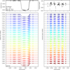 |
Fig. 1 White light curve of HD 209458 b’s HST/WFC3 transit with the best-fit transit model (upper left panel) and residuals of the fit (upper right panel), as well as the spectral light curves (lower left panel; offset) with fit transit models and the corresponding residuals (lower right panel). |
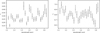 |
Fig. 2 Variation in the fitted model_ramp parameters r1 and r2 (cf. Eq. (1)) with wavelength. The dots represent best-fit values in each wavelength bin with 1 σ errors from the posterior. Both r1 and r2 are clearly not wavelength-independent. |
Parameters for the spectroscopic light curve fits with assigned uniform priors (U).
2.2 Recreation of the Deming et al. (2013) data reduction method
In the original reduction, we noticed a zig-zag pattern (see Fig. 3) of alternating higher and lower transit depths between subsequent exposures, particularly at shorter wavelengths. This pattern was not present in the original transmission spectrum by Deming et al. (2013). To investigate the origin of this pattern, we recreated the reduction method used by Deming et al. (2013). As they were the first to report the extraction of an atmospheric transmission spectrum from spatially scanned transit observations of an exoplanet, they employed a slightly different method than the one commonly used today. The main differences between the two methods are explained below.
After extracting a 1D spectrum at each exposure, as in the current method, Deming et al. (2013) convolved each of these spectra with a Gaussian kernel of FWHM = 4 pix to reduce the effect of undersampling the spectrum and avoid degradation of the spectral resolution. The template spectrum for the wavelength correction was not derived from a modelled stellar spectrum, but through averaging the spectra one hour before the start of the transit and one hour after the end. Furthermore, all individual spectra were resampled to a finer wavelength sampling and then interpolated to a common wavelength solution. At each exposure, the template spectrum was fit separately to the individual spectrum via least-squares fitting by shifting it in wavelength and stretching it in flux. The residuals of this fit, i.e. fit minus template spectrum, were binned into the same 28 wavelength channels, as mentioned earlier. We then fit an eclipse model from the batman code (Kreidberg 2015) and a linear base-line to these residuals. Here, the eclipse model was used instead of the transit model to fit declines and inclines of the flux in the residuals. The transmission spectrum was generated by adding the eclipse depth at each binned wavelength to the white light transit depth. We were successful in recreating this method.
While working on this method, we realised that smoothing the individual spectra at each exposure with a Gaussian kernel was the crucial step to avoid the zig-zag pattern, which also appeared in the transmission spectrum generated with the reduction method of Deming et al. (2013) when the smoothing was turned off. As a result, we implemented this step in the PACMAN code. Deming et al. (2013) included this additional smoothing originally to reduce undersampling effects due to changes in the stellar line shapes during the transit. These could also be the reason for the pattern we see in our transmission spectra before adding the Gaussian convolution. However, Deming et al. (2013) noted the most pronounced differences near strong stellar lines, for example Paschen-β (λ = 1.28 μm), and we do not see strong effects there (see Fig. 3). Nevertheless, the added Gaussian convolution step helps to avoid the zig-zag pattern. Figure 3 shows a comparison of the model_ramp spectra before and after applying the Gaussian convolution, and Fig. 4 shows the transmission spectrum obtained using both models for the instrument systematics compared to the transmission spectrum of Deming et al. (2013).
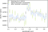 |
Fig. 3 Comparison of HST/WFC3 transmission spectra with (blue) and without (green) applying the additional Gaussian convolution (see Sect. 2.2) in the data reduction. Both spectra use the model_ramp model. The green spectrum without the additional smoothing step shows a zig-zag pattern of alternating transit depths between subsequent exposures. The grey spectrum is from Deming et al. (2013) for comparison. |
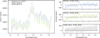 |
Fig. 4 Comparison of HST/WFC3 transmission spectra for three different data reduction and fitting methods for HD 209458 b. The blue spectrum uses exponential functions to fit the systematics at the beginning of each orbit (model_ramp fit), whereas the green spectrum assumes wavelength independent systematics (divide_white fit). The grey spectrum is the original transmission spectrum published by Deming et al. (2013). The right panels show the differences between all three spectra. Noticeable is the linear trend with wavelength in the residuals for all three cases. |
3 Atmospheric retrievals of the newly reduced HST spectrum
Atmospheric retrievals are a powerful tool for analysing transmission spectra. For this study, we used petitRADTRANS, which incorporates the pymultinest (Buchner et al. 2014) nested sampling algorithm, to perform the atmospheric retrievals. The chosen models and the parameter set-up are introduced in the following Sect. 3.1. In Sect. 3.2 we summarise the results of the atmospheric retrieval analyses of the newly reduced HST/WFC3 transmission spectrum.
3.1 Model and parameter set-up
Several previous studies (e.g. Madhusudhan et al. 2014a; Benneke 2015; Barstow et al. 2017; MacDonald & Madhusudhan 2017, and Xue et al. 2024) have run retrievals on HD 209458 b’s transmission spectrum. The results, especially the water abundances obtained, were contradictory, as mentioned earlier. In the following, we describe the model and parameter set-up for atmospheric retrievals in this paper. As stated above, we used the model_ramp transmission spectrum for the retrievals. For comparison, we also ran retrievals on the original spectrum published by Deming et al. (2013). Using the planetary radius Rpl = 1.359 RJup and mass Mpl = 0.682 MJup (Bonomo et al. 2017), we retrieved a reference pressure Pref at which this radius and mass are reached, together with the other model parameters. This method has the advantage of using directly measurable quantities for the planet instead of the inferred gravity log (g).
We assumed an isothermal atmosphere for the planet and tested cloud-free models, patchy clouds, and a completely opaque grey cloud deck. Table 2 shows the parameter inputs adopted for the forward models, and Table 3 provides an overview of all the cloud models tested in this study. Table 4 provides a list of all retrievals run on the spectra with the results.
We used a free chemistry retrieval approach with H2O, CH4, NH3, HCN, and Na as line-absorbing species in the atmosphere, given by the main absorbers in the wavelength range of the transmission spectrum and the claimed findings of previous work (MacDonald & Madhusudhan 2017; Tsiaras et al. 2018; Xue et al. 2024). We used a model resolution of 200, which is sufficient for the resolution of our data (less than R = 100). For the rebinning of the opacities, we used the Exo_k package (Leconte 2021) in the correlated-k mode of petitRADTRANS. We used the opacities calculated from the Pokazatel (Polyansky et al. 2018) line list for H2O, HITEMP (Hargreaves et al. 2020) for CH4, the lists by Coles et al. (2019) for NH3 and by Harris et al. (2006) for HCN, and the Piskunov et al. (1995) line list for Na. For all the line species, we adopted log-uniform priors with mass fraction abundance limits of 10−12 to 1. Hydrogen and helium were assumed to be responsible for Rayleigh scattering in the atmosphere and also to contribute to the continuum opacities via collision-induced absorption of H2 − H2 and H2 − He. We assumed an atmosphere consisting mainly of hydrogen and helium with mass mixing ratios of 0.74 and 0.24, respectively. Due to the fairly small size of the retrievals, we used 1000 live points.
Input parameters for the retrievals of the HST spectra.
Overview of the different cloud models used in this study.
3.2 Retrieval results
A list of all retrievals on the different HST spectra can be found in Table 4. To robustly estimate the various parameters and compare the different models, we used a Bayesian framework. The Bayesian evidence quantifies the suitability of the tested atmospheric model to the data (MacDonald & Madhusudhan 2017). The Bayes factor Zref/Z gives an indication of which model is favoured, and factors of 3, 12, and 150 are often interpreted respectively as weak, moderate, and strong detections of the reference over the other model (Trotta 2008; Benneke & Seager 2013). Bayes factors can also be transformed into σ-significances, using Eqs. (8) and (9) in Benneke & Seager (2013). With this approach, we first determined the best-fitting atmospheric model from cloudy, patchy, or no cloud models, using all line species in the retrievals. As Table 4 shows, all three models have similar Bayesian evidence and Bayes factors, which are too small to even weakly distinguish one model from the others. The best-fit spectra for these models are shown in Fig. 5. The clouds expected on a planet similar to HD 209458 b could consist of Fe, Ni, Al2O3, Mg2SiO4, MgSiO3, MgFeSiO4, SiC, TiO2, or MnS (Burrows & Sharp 1999; Benneke 2015; Mbarek & Kempton 2016; Woitke et al. 2018; Kitzmann et al. 2024) assuming a solar-composition gas.
In the further analysis of this spectrum, we used the cloud-free model as a reference because it has fewer parameters than the cloudy or patchy clouds model. As the Bayes factors do not clearly distinguish between them, we prefer the simplest possible model, which also has the lowest ![Mathematical equation: $\[\chi_{red}^{2}\]$](/articles/aa/full_html/2025/08/aa55577-25/aa55577-25-eq6.png) value. The different line-absorbing species were tested by running retrievals in which one absorber was left out to determine how well it was detected. As Table 4 shows, H2O was the only species detected, with a significance of 4σ (calculated from Bayes factors). None of the other absorbers are significantly detected. Moreover, we compared the full model with all absorbing species to one that included only water; we found that the latter was moderately favoured by a Bayes factor of 5, further emphasising the fact that water is the only relevant line absorber in this wavelength range. The best-fit spectra for several of the tested models are shown in Fig. 6. H2O is clearly recognisable as the main absorbing molecular species in this wavelength range.
value. The different line-absorbing species were tested by running retrievals in which one absorber was left out to determine how well it was detected. As Table 4 shows, H2O was the only species detected, with a significance of 4σ (calculated from Bayes factors). None of the other absorbers are significantly detected. Moreover, we compared the full model with all absorbing species to one that included only water; we found that the latter was moderately favoured by a Bayes factor of 5, further emphasising the fact that water is the only relevant line absorber in this wavelength range. The best-fit spectra for several of the tested models are shown in Fig. 6. H2O is clearly recognisable as the main absorbing molecular species in this wavelength range.
To combine the results for the parameters of all different retrieval models, we applied the Bayesian model averaging (BMA) method (Nixon et al. 2024; Nasedkin et al. 2024b). For parameters that are shared between several models, we obtained a combined posterior distribution. For the calculation, the posterior distributions of different models were summed with weights according to their Bayesian evidence (see Eqs. (12)–(14) in Nasedkin et al. 2024b). This resulted in more robust uncertainties for every parameter as the uncertainties from the data and prior distribution as well as the model uncertainty itself were taken into account. To avoid bias in the results, all the models used in the averaging have to be conceptually different. Therefore, we averaged only models with different cloud treatments, including all species, since most line absorbers do not have constrained abundances. Averaging over all models would possibly bias the results towards the cloud-free case, as these make up the majority of the models. In Fig. A.2, we show the averaged posterior distributions for the parameters present in most models. Since the abundances of CH4, NH3, HCN, and Na are not constrained, we only report 3σ upper limits of log(χCH4) = −3.43, log(χNH3) = −2.62, log(χHCN) = −2.66, and log(χNa) = −2.01. We could not reproduce former detections of methane or nitrogenous species, as claimed in MacDonald & Madhusudhan (2017). The retrieved values for all parameters can be found in the Appendix, Table A.1.
For comparison, we ran the same retrievals using the original transmission spectrum published by Deming et al. (2013). The retrievals show similar results for the H2O abundance, but the ![Mathematical equation: $\[\chi_{\text {red }}^{2}\]$](/articles/aa/full_html/2025/08/aa55577-25/aa55577-25-eq22.png) values of the retrievals using our data reduction are much lower (1.33 vs. 1.99 for the preferred cloud-free, only H2O model, cf. Table 4). This shows that the new data reduction indeed has an effect and might change the results, as we obtain better model fits to our transmission spectrum.
values of the retrievals using our data reduction are much lower (1.33 vs. 1.99 for the preferred cloud-free, only H2O model, cf. Table 4). This shows that the new data reduction indeed has an effect and might change the results, as we obtain better model fits to our transmission spectrum.
Figure 7 shows that we retrieved a Bayesian averaged water abundance of log(χH2O) = ![Mathematical equation: $\[-5.22_{-0.40}^{+2.37}\]$](/articles/aa/full_html/2025/08/aa55577-25/aa55577-25-eq23.png) from the HST spectrum. This is well below solar abundance, and is consistent with several previous studies (Madhusudhan et al. 2014a; Barstow et al. 2017; MacDonald & Madhusudhan 2017). The low water abundance can be explained by the use of cloud-free models when retrieving the HST spectrum. Since the water feature in the spectrum is quite small and in most models no clouds are present to suppress it, a lower water abundance is needed to fit the data than when a cloud is present (Welbanks & Madhusudhan 2021). This trend can be seen in Table 4 and in Table 6 for the joint HST-JWST retrievals. As Madhusudhan et al. (2014b) state, such a sub-solar water abundance could be explained by a significant sub-solar metallicity; alternatively, a highly super-solar C/O would be required. From the JWST and the joint HST-JWST spectrum (see Sect. 4.2) as well as other hot Jupiter datasets (e.g. Ahrer et al. 2023; Fu et al. 2024; Bell et al. 2024), we expect a cloudy rather than a clear atmosphere for HD 209458 b. Therefore, we also included retrievals using the cloudy model and just H2O as a line absorber (Table 4). The water abundance matches those of the other retrievals and is between the cloud-free and cloudy results when we used all species in the retrievals (see Table 4). Even though the cloudy models are not favoured by the Bayesian evidence or the
from the HST spectrum. This is well below solar abundance, and is consistent with several previous studies (Madhusudhan et al. 2014a; Barstow et al. 2017; MacDonald & Madhusudhan 2017). The low water abundance can be explained by the use of cloud-free models when retrieving the HST spectrum. Since the water feature in the spectrum is quite small and in most models no clouds are present to suppress it, a lower water abundance is needed to fit the data than when a cloud is present (Welbanks & Madhusudhan 2021). This trend can be seen in Table 4 and in Table 6 for the joint HST-JWST retrievals. As Madhusudhan et al. (2014b) state, such a sub-solar water abundance could be explained by a significant sub-solar metallicity; alternatively, a highly super-solar C/O would be required. From the JWST and the joint HST-JWST spectrum (see Sect. 4.2) as well as other hot Jupiter datasets (e.g. Ahrer et al. 2023; Fu et al. 2024; Bell et al. 2024), we expect a cloudy rather than a clear atmosphere for HD 209458 b. Therefore, we also included retrievals using the cloudy model and just H2O as a line absorber (Table 4). The water abundance matches those of the other retrievals and is between the cloud-free and cloudy results when we used all species in the retrievals (see Table 4). Even though the cloudy models are not favoured by the Bayesian evidence or the ![Mathematical equation: $\[\chi_{\text {red }}^{2}\]$](/articles/aa/full_html/2025/08/aa55577-25/aa55577-25-eq24.png) values from the HST data alone, they are probably the most realistic models for HD 209458 b’s atmosphere. They also show a clear tendency (cf. Table 4) to higher H2O abundances, which we would expect. Since earlier analyses of the HST dataset mostly favoured lower H2O abundances, similar to our cloud-free models and in contradiction to expectations, our study clearly shows the limitations of obtaining robust results when using only HST data due to the limited wavelength coverage and precision. Here, adding JWST data with better precision and broader wavelength coverage leads to more robust results (see also Sect. 4.2). In addition, we caution against using only Bayesian evidence as a criterion to decide on the most likely models, as it may favour simpler but not necessarily more realistic models. Planetary atmospheres are inherently complex and might not be best described by simpler models, even if statistically preferred.
values from the HST data alone, they are probably the most realistic models for HD 209458 b’s atmosphere. They also show a clear tendency (cf. Table 4) to higher H2O abundances, which we would expect. Since earlier analyses of the HST dataset mostly favoured lower H2O abundances, similar to our cloud-free models and in contradiction to expectations, our study clearly shows the limitations of obtaining robust results when using only HST data due to the limited wavelength coverage and precision. Here, adding JWST data with better precision and broader wavelength coverage leads to more robust results (see also Sect. 4.2). In addition, we caution against using only Bayesian evidence as a criterion to decide on the most likely models, as it may favour simpler but not necessarily more realistic models. Planetary atmospheres are inherently complex and might not be best described by simpler models, even if statistically preferred.
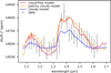 |
Fig. 5 Comparison of best-fit spectra with different cloud assumptions. The retrieval uses the model_ramp fit HST/WFC3 spectrum (grey dots). All three retrievals include all tested absorbing species (see Table 4). The red spectrum is cloud-free, the blue one cloudy, and the orange spectrum is the best fit for patchy clouds. |
Summary of all retrievals run on the HST spectra.
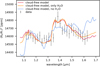 |
Fig. 6 Comparison of best-fit cloud-free spectra for retrievals of the model_ramp fit HST/WFC3 spectrum. The red spectrum is the same as in Fig. 5. The orange spectrum is the best fit for the model with the highest Bayesian evidence (clear atmosphere and only H2O as line absorber). The light blue spectrum is the model that does not contain water as an absorber. |
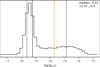 |
Fig. 7 Bayesian model averaged posterior distribution for H2O from the HST/WFC3 retrievals. The black line indicates the median of the distribution, and the dashed lines are the ±34.1% confidence regions. The orange lines shows the solar value (log(χH2O) = −3.70) at 1 mbar and 1200 K. Since most of the models used for the BMA do not include clouds, the results are more heavily weighted towards the cloud-free solution, and therefore lower H2O abundances (see text). |
4 Atmospheric retrievals of the combined HST-JWST spectrum
As shown in Fig. 4, the new data reduction used in this study yields slightly different results compared to the original spectrum, which made it worthwhile to conduct a joint atmospheric analysis of this planet again. The broader wavelength coverage of the combined dataset also allowed us to test a broader range of retrieval approaches, including different and more complex cloud models, and species that do not absorb in the HST wavelength range.
4.1 Joint retrieval set-up
JWST/NIRCam operates in a wavelength range different from HST’s WFC3, so we included CO2 and CO in the list of line absorbers for the joint retrieval. Because several years passed between the observations, differences in stellar activity cannot be excluded. The two instruments are also affected by different systematics. To account for these differences, we also introduced an optional offset with a Gaussian prior (which covers the offset retrieved by Xue et al. 2024) for the HST data relative to the JWST data in the parameters. For the temperature, we adopted a broader uniform prior and included the planet’s mass and radius (Bonomo et al. 2017) along with the associated errors as retrieved parameters in the set-up. It was not feasible to retrieve the HST data alone while including these additional free parameters, due to the limited number of data points. The results we obtained were not influenced by the choice of narrow uniform priors for the planet’s mass and radius. We obtained comparable results for all the parameters when using wider Gaussian priors, with the exception of the reference pressure, as was expected. Since the retrievals using the narrow priors have a shorter runtime, we continued using them. For the atmospheric model, we used the same isothermal transmission model as described in Sect. 3.1, with the same line lists for the absorbers and the HITEMP (Hargreaves et al. 2020) list for CO and the list by Yurchenko et al. (2020) for CO2. The input parameters for the joint retrievals are provided in Table 5. Due to the larger dataset, we used 4000 live points for the joint retrievals. We ran the retrievals on the model_ramp HST data, combined with the JWST/NIRCam data published by Xue et al. (2024).
Input parameters for the joint retrievals on the combined HSTJWST spectra.
4.2 Joint retrieval results
Table 6 presents the results of the combined retrievals. To determine the best model, we used the approach described in Sect. 3.2. Since the cloudy model has a slightly higher Bayesian evidence log (Z) than the patchy cloud model, we selected the cloudy model for further analysis as it also has one fewer parameter, one that is not strictly necessary to fit the data. Both models show a reasonably strong preference (3.6 σ) for a clear atmosphere. Best-fit spectra for all three models are shown in Fig. 8.
For the cloudy models, we evaluated which line species are required to fit the data properly. By comparing the Bayesian evidence, only H2O and CO2 can be robustly claimed to be detected (Table 6). The cloudy model with only these two molecules as line absorbers has the highest Bayesian evidence of all tested models. This further supports the conclusion that all other absorbing species are unnecessary for interpreting the data. Water is detected at over 14σ (for the corresponding Bayes factors, see Table 6) with a log volume mixing ratio of log(χH2O) = ![Mathematical equation: $\[-4.47_{-0.50}^{+1.26}\]$](/articles/aa/full_html/2025/08/aa55577-25/aa55577-25-eq25.png) in the cloudy model and log(χH2O) =
in the cloudy model and log(χH2O) = ![Mathematical equation: $\[-4.51_{-0.48}^{+1.15}\]$](/articles/aa/full_html/2025/08/aa55577-25/aa55577-25-eq26.png) in the model that only includes H2O and CO2. CO2 is detected at more than 7σ (see Table 6) with a log volume mixing ratio of log(χCO2) =
in the model that only includes H2O and CO2. CO2 is detected at more than 7σ (see Table 6) with a log volume mixing ratio of log(χCO2) = ![Mathematical equation: $\[-7.64_{-0.37}^{+1.18}\]$](/articles/aa/full_html/2025/08/aa55577-25/aa55577-25-eq27.png) in the cloudy model and log(χCO2) =
in the cloudy model and log(χCO2) = ![Mathematical equation: $\[-7.67_{-0.36}^{+1.07}\]$](/articles/aa/full_html/2025/08/aa55577-25/aa55577-25-eq28.png) in the model that only includes H2O and CO2. The model with the highest evidence (clouds and only H2O and CO2 as line absorbers) is preferred over the one that includes all other species tested by 3.1σ. All other tested species are not required to fit the spectrum with significances ranging from 2.8 to 3.0 σ, and they do not show constrained posterior distributions. Therefore, we only report upper limits for the volume mixing ratios of all these species (see Sect. 4.4). Figure 9 shows the best-fit spectra of some of the tested models, and Fig. A.4 presents the corner plot for the model with the highest Bayesian evidence, the cloudy model including only H2O and CO2.
in the model that only includes H2O and CO2. The model with the highest evidence (clouds and only H2O and CO2 as line absorbers) is preferred over the one that includes all other species tested by 3.1σ. All other tested species are not required to fit the spectrum with significances ranging from 2.8 to 3.0 σ, and they do not show constrained posterior distributions. Therefore, we only report upper limits for the volume mixing ratios of all these species (see Sect. 4.4). Figure 9 shows the best-fit spectra of some of the tested models, and Fig. A.4 presents the corner plot for the model with the highest Bayesian evidence, the cloudy model including only H2O and CO2.
Tsai et al. (2023) detected photochemically produced SO2 in the atmosphere of the hot Jupiter WASP-39 b. Since this molecule could also be present in the atmospheres of other hot Jupiters, we included it as an absorber in the analysis, using the line list from Underwood et al. (2016). We only retrieved a 3σ upper limit of log(χSO2) = −5.93 for the volume mixing ratio. The Bayes factor also disfavours the inclusion of SO2 in the species required to describe the atmosphere of HD 209458 b with a significance of 1.82σ compared to the cloudy model, and 3.3σ compared to the cloudy model that only includes H2O and CO2, which has the highest Bayesian evidence.
We also tested H2S, another sulphur-bearing species expected at the planetary temperature of HD 209458 b. Xue et al. (2024) reported a tentative hint of its presence in the atmosphere, and H2S was previously detected on the hot Jupiter HD 189733 b (Fu et al. 2024). Our retrievals using the ExoMol line list (Azzam et al. 2016) do not yield a constrained posterior distribution for H2S. We obtained a 3σ upper limit for its volume mixing ratio of log(χH2S) = −4.00, with Bayesian evidence favouring the cloudy model without it (see Table 6).
The measured water abundances from the joint spectra are higher than those from the retrievals of the HST spectrum alone. Since the spectral range of the combined HST-JWST spectrum is wider than previously analysed (see Sect. 3) and contains an additional water feature around 2.8 μm (cf. Fig. 11), the water abundance is likely more easily constrainable and more reliable than the result obtained using only HST data. The results for all the parameters and retrievals can be found in Tables A.2 and A.3.
Summary of all retrievals run on the combined HST-JWST spectra.
4.3 Retrievals with more complex clouds
Since the cloudy model and patchy cloud model have almost identical Bayesian evidence, and the assumptions for the clouds are quite simple–a grey cloud deck at a retrieved pressure Pcloud in the atmosphere–we also tested a more complex model for the clouds. We used the model described in Dyrek et al. (2023, Sect. 3.2 of the supplementary materials). Their model employs the following description for the cloud opacity κcloud:
![Mathematical equation: $\[\begin{array}{lr}\kappa_{\text {cloud }}=\frac{\kappa_{\text {base }}}{1+\left(\frac{\lambda}{\lambda_0}\right)^p}\left(\frac{P}{P_{\text {base }}}\right)^{f_{\text {sed }}} & \text { if } P<P_{\text {base }} \text { and } \\\kappa_{\text {cloud }}=0 & \text { if } P \geq P_{\text {base}}.\end{array}\]$](/articles/aa/full_html/2025/08/aa55577-25/aa55577-25-eq62.png) (2)
(2)
Here λ represents the wavelength in micrometres and P the pressure in bars. The free parameters also include the opacity at the cloud base κbase, the reference wavelength λ0, the pressure at the cloud base Pbase, the power-law coefficient p (which describes the opacity dependence on the wavelength at λ ≫ λ0), and the sedimentation efficiency of the cloud particles fsed. The input values for these cloud parameters are listed in Table 7. For all other retrieved parameters, we used the same priors as before (cf. Table 5), with the exception of the cloud pressure log (Pcloud), which was excluded.
The results of the retrievals found using this more complex cloud model are shown in Table 6. All of these models exhibit slightly lower Bayesian evidence than the simple grey cloud-deck model, despite having more free parameters to adjust. Therefore, the more complex model is not necessary to describe the clouds of HD 209458 b. Complex cloud and complex patchy cloud models are not significantly ruled out compared to the simple cloud model, with significance levels of 2.1 and 1.6σ, respectively. On the other hand, the more complex cloud model that includes only H2O and CO2 as line absorbers is ruled out by 3.6σ in comparison to the simple cloud model that includes only H2O and CO2. Notably, the retrievals with the more complex cloud model yield higher water abundances. This can be explained by the fact that for the more complex model the cloud opacity extends above the cloud base at Pbase and obscures the water to a greater degree. For the simple cloud model, everything below the cloud location at Pcloud is obscured, but the atmosphere is clear above it. Figure 8 also shows the best-fit spectra with the more complex cloud model compared to those using the simple cloud approximation of a grey opacity at a retrieved pressure. The results for all parameters and retrievals can be found in Tables A.2 and A.3.
 |
Fig. 8 Comparison of best-fit spectra for retrievals of the joint HST-JWST spectrum using different cloud models. The fits include all tested absorbing species except for SO2 and H2S (see Table 6). The red spectrum is cloud-free, the blue spectrum is cloudy, and the orange spectrum is the best fit for patchy clouds. The dashed spectra are the best fits using the more complex cloud model described in Sect. 4.3. We also fit for an offset between the HST and JWST data, which is visible by eye in the figure (for details, see Tables A.2 and A.3). |
4.4 Results of the Bayesian model averaging
As for the HST spectral fits, we used Bayesian model averaging to account for the model uncertainty in the retrieved parameters. To avoid biases in the process, we averaged the cloud-free, cloudy, patchy clouds, complex clouds, and complex patchy clouds model, excluding the quite similar cloudy models in which just one species was left out. Since most of the species are not actually detectable, this would lead to a combination of the same cloudy model several times. Figure A.3 shows the Bayesian model averaged posteriors for the parameters present in most of the models tested. From our uniform cloud models tested, we report a grey cloud deck at a Bayesian model averaged pressure of Pcloud = ![Mathematical equation: $\[1.74_{-1.58}^{+4.01}\]$](/articles/aa/full_html/2025/08/aa55577-25/aa55577-25-eq64.png) · 10−2 bar in the atmosphere of HD 209458 b. The averaged water abundance corresponds to a volume mixing ratio of log(χH2O) =
· 10−2 bar in the atmosphere of HD 209458 b. The averaged water abundance corresponds to a volume mixing ratio of log(χH2O) = ![Mathematical equation: $\[-3.91_{-0.86}^{+1.05}\]$](/articles/aa/full_html/2025/08/aa55577-25/aa55577-25-eq65.png) (see Fig. 10). The solar water abundance at a representative pressure level of 1 mbar is −3.70. Therefore, our measured value agrees with the solar abundance within 1σ. CO2 is detected with an abundance of log(χCO2) =
(see Fig. 10). The solar water abundance at a representative pressure level of 1 mbar is −3.70. Therefore, our measured value agrees with the solar abundance within 1σ. CO2 is detected with an abundance of log(χCO2) = ![Mathematical equation: $\[-7.16_{-0.76}^{+1.02}\]$](/articles/aa/full_html/2025/08/aa55577-25/aa55577-25-eq66.png) (see Fig. 10), which is also consistent with solar abundances within 1σ. No other species tested show constrained posterior distributions, and therefore we can only provide 3σ upper limits on abundances. These are log(χCH4) = −6.35, log(χNH3) = −5.16, log(χHCN) = −5.99, log(χNa) = −1.87, and log(χCO) = −3.26. Comparing the results of the joint HST-JWST spectrum with the averaged abundances of the different species with the solar values at 1 mbar, we find that almost all of them (with the exception of CO) are consistent within 1σ with the solar values (Fig. A.3, Fig. 10), as expected from planet formation models (Öberg & Bergin 2016; Booth et al. 2017). This challenges the results of Madhusudhan et al. (2014a) and MacDonald & Madhusudhan (2017), while our results are in agreement with those of Line et al. (2016), Pinhas et al. (2019), Welbanks et al. (2019), Tsiaras et al. (2018) and Welbanks & Madhusudhan (2021). One caveat is that all of these previous studies based their results on the HST spectrum alone. Our measured upper limits on the abundances of CH4, NH3, and HCN are all lower, but still consistent with the corresponding results of Xue et al. (2024). Similarly to Xue et al. (2024), our findings do not confirm the high-resolution ground-based spectroscopy results of Giacobbe et al. (2021), who reported detections of CH4, NH3, HCN, and C2H2. These findings were also already refuted by Blain et al. (2024a).
(see Fig. 10), which is also consistent with solar abundances within 1σ. No other species tested show constrained posterior distributions, and therefore we can only provide 3σ upper limits on abundances. These are log(χCH4) = −6.35, log(χNH3) = −5.16, log(χHCN) = −5.99, log(χNa) = −1.87, and log(χCO) = −3.26. Comparing the results of the joint HST-JWST spectrum with the averaged abundances of the different species with the solar values at 1 mbar, we find that almost all of them (with the exception of CO) are consistent within 1σ with the solar values (Fig. A.3, Fig. 10), as expected from planet formation models (Öberg & Bergin 2016; Booth et al. 2017). This challenges the results of Madhusudhan et al. (2014a) and MacDonald & Madhusudhan (2017), while our results are in agreement with those of Line et al. (2016), Pinhas et al. (2019), Welbanks et al. (2019), Tsiaras et al. (2018) and Welbanks & Madhusudhan (2021). One caveat is that all of these previous studies based their results on the HST spectrum alone. Our measured upper limits on the abundances of CH4, NH3, and HCN are all lower, but still consistent with the corresponding results of Xue et al. (2024). Similarly to Xue et al. (2024), our findings do not confirm the high-resolution ground-based spectroscopy results of Giacobbe et al. (2021), who reported detections of CH4, NH3, HCN, and C2H2. These findings were also already refuted by Blain et al. (2024a).
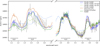 |
Fig. 9 Comparison of best-fit spectra for retrievals of the joint HST-JWST spectrum using different molecular absorbers and a grey cloud. The orange spectrum is the best-fit case from the model with the highest Bayesian evidence: a grey cloud and only H2O and CO2 as line absorbers. The light blue dashed spectrum does not include water as an absorber, whereas the light green dashed spectrum is without CO2. The dark green spectrum is the best fit of the cloudy+CO prior model (see Sect. 4.5). As in Fig. 8, there is a vertical offset between the HST and JWST data. |
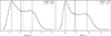 |
Fig. 10 Bayesian model averaged posterior distributions for H2O (left) and CO2 (right). The black line indicates the median of the distributions, and the dashed lines are the ±34.1% confidence regions. The orange lines show the solar value of log(χH2O) = −3.70 and log(χCO2) = −7.05 at 1 mbar and 1200 K. |
4.5 Metallicities and C/O values
To compare our free retrieval results with those of previous work that assumed chemical equilibrium, we calculated the metallicity and C/O from the volume mixing ratio posterior distributions of our cloudy retrieval. As we only account for H2, He, and the line-absorbing species tested in the retrievals, the metallicity obtained is a lower estimate of the actual atmospheric metallicity of HD 209458 bat ~1 mbar. The C/O was calculated from the C/H and O/H that we obtained from the retrieved volume mixing ratios. Our results indicate a metal-depleted atmosphere (atmospheric metallicity of [M/H] = ![Mathematical equation: $\[-1.35_{-0.73}^{+1.25}\]$](/articles/aa/full_html/2025/08/aa55577-25/aa55577-25-eq67.png) ), which is consistent with solar values at the ~1 σ level. We also derived an extremely low C/O of
), which is consistent with solar values at the ~1 σ level. We also derived an extremely low C/O of ![Mathematical equation: $\[1.33_{-0.70}^{+4.79}\]$](/articles/aa/full_html/2025/08/aa55577-25/aa55577-25-eq68.png) · 10−3. The results are likely driven by the low CO abundance (3 σ upper limit of log(χCO) = −3.26) measured in our spectra and the absence of CH4 (3σ upper limit of log(χCH4) = −6.35). The apparent depletion of CO relative to the solar value may be an artefact of the clouds, which mute the features in the CO wavelength band through strong absorption (visible in Fig. 11). Furthermore, Fig. 11 clearly shows that in the wavelength range where CO could be detected (4.4–5.2 μm) it is additionally obscured by stronger water absorption. Therefore, no features due to CO absorption are visible. In addition, all features from absorbing species other than H2O and CO2 are hidden beneath the cloud deck and consequently are not easy to constrain, even though their opacity still contributes to the total measured opacity. Additionally, the figure illustrates the muting effect of the grey cloud deck on the individual absorbing features, especially those due to water.
· 10−3. The results are likely driven by the low CO abundance (3 σ upper limit of log(χCO) = −3.26) measured in our spectra and the absence of CH4 (3σ upper limit of log(χCH4) = −6.35). The apparent depletion of CO relative to the solar value may be an artefact of the clouds, which mute the features in the CO wavelength band through strong absorption (visible in Fig. 11). Furthermore, Fig. 11 clearly shows that in the wavelength range where CO could be detected (4.4–5.2 μm) it is additionally obscured by stronger water absorption. Therefore, no features due to CO absorption are visible. In addition, all features from absorbing species other than H2O and CO2 are hidden beneath the cloud deck and consequently are not easy to constrain, even though their opacity still contributes to the total measured opacity. Additionally, the figure illustrates the muting effect of the grey cloud deck on the individual absorbing features, especially those due to water.
To account for hidden CO, we fit the data again using a ground-based high-resolution CO abundance measurement from Brogi & Line (2019) as a prior in a retrieval with a grey cloud deck (uniform prior U(−3.5, 0.0) for the CO mass fraction). From here on, this model is referred to as cloudy+CO prior. In the ground-based observations CO is visible, even if we cannot detect it in the JWST data, because for the high-resolution result many individual absorption lines around 2.3 μm are combined for the final detection (Brogi & Line 2019). In addition, at this wavelength, water does not absorb as strongly (cf. Fig. 11). The best-fit spectrum and the corner plot are shown in Fig. 9 and Fig. A.5, respectively. The logarithmic Bayesian evidence for this retrieval is 365.4 ± 0.2, and is therefore disfavoured by 2.6σ compared to the cloudy retrieval with the broader CO prior; however, the higher retrieved CO volume mixing ratio of log(χCO) = ![Mathematical equation: $\[-4.15_{-0.30}^{+0.51}\]$](/articles/aa/full_html/2025/08/aa55577-25/aa55577-25-eq69.png) shifts the metallicity and C/O distribution to more physically reasonable values of [M/H] =
shifts the metallicity and C/O distribution to more physically reasonable values of [M/H] = ![Mathematical equation: $\[0.10_{-0.40}^{+0.41}\]$](/articles/aa/full_html/2025/08/aa55577-25/aa55577-25-eq70.png) for the metallicity and
for the metallicity and ![Mathematical equation: $\[0.054_{-0.034}^{+0.080}\]$](/articles/aa/full_html/2025/08/aa55577-25/aa55577-25-eq71.png) for the C/O (Fig. 12). The metallicity is consistent with the solar value and the CO abundance is slightly below solar, but the C/O is significantly sub-solar, indicating an atmosphere rich in oxygen and depleted in carbon.
for the C/O (Fig. 12). The metallicity is consistent with the solar value and the CO abundance is slightly below solar, but the C/O is significantly sub-solar, indicating an atmosphere rich in oxygen and depleted in carbon.
 |
Fig. 11 Contribution of the opacities of line-absorbing species to the transmission spectrum. The best-fit spectrum shows the cloudy+CO prior model (see text). The absorption features of H2O and CO2 are clearly visible, for the latter due to its strong absorption even though the abundance is low (see Fig. 10). |
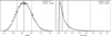 |
Fig. 12 Metallicity (left) and C/O (right) distribution calculated from the posterior distributions of the cloudy+CO prior retrieval. The black solid lines indicate the median, and the dashed lines depict the ±34.1% confidence regions. The dotted line shows the 3σ upper limit of 0.454 for C/O. The same calculations without a tight CO prior yielded a very sub-solar metallicity of [M/H] = |
![Mathematical equation: $\[-1.35_{-0.73}^{+1.25}\]$](/articles/aa/full_html/2025/08/aa55577-25/aa55577-25-eq72.png)
![Mathematical equation: $\[1.33_{-0.70}^{+4.79}\]$](/articles/aa/full_html/2025/08/aa55577-25/aa55577-25-eq73.png)
4.6 Comparison with previous work
In Xue et al. (2024), the authors presented results for equilibrium chemistry retrievals of the JWST/NIRCam data (and one combined HST-JWST retrieval), including the planet’s radius (at a pressure of 1 bar), temperature, metallicity, C/O, the pressure at the cloud top, the cloud fraction, and the mixing ratios of CH4, NH3, C2H2, and HCN. The only relevant absorbing species they identified were H2O and CO2, with a tentative detection of H2S. They find a metallicity of [M/H] = ![Mathematical equation: $\[0.63_{-0.24}^{+0.31}\]$](/articles/aa/full_html/2025/08/aa55577-25/aa55577-25-eq74.png) and a C/O value of
and a C/O value of ![Mathematical equation: $\[0.19_{-0.09}^{+0.14}\]$](/articles/aa/full_html/2025/08/aa55577-25/aa55577-25-eq75.png) . Their retrieval favours a patchy cloud model with a covering fraction of around 70%.
. Their retrieval favours a patchy cloud model with a covering fraction of around 70%.
In this work we focus on free retrievals that do not impose equilibrium chemistry. Our combined HST and JWST free chemistry retrievals yield broadly similar results to Xue et al. (2024), with confident detections of H2O, CO2, and clouds. However, even with the CO prior, our inferred metallicity and C/O are still lower than those reported by Xue et al. (2024) at 2.4 and 1.7σ, respectively. One reason for this difference could be that the equilibrium chemistry retrieval of Xue et al. (2024) is sensitive to the shape of the previously published HST spectrum. We find that our results are more consistent with Xue et al. (2024) when they analyse the JWST data alone. In this case, their retrieved C/O value of ![Mathematical equation: $\[0.08_{-0.05}^{+0.09}\]$](/articles/aa/full_html/2025/08/aa55577-25/aa55577-25-eq76.png) for this dataset alone agrees within 1 σ with our result.
for this dataset alone agrees within 1 σ with our result.
Some other differences include no evidence for H2S in our retrievals; instead, we find a 3σ upper limit of log(χH2S) = −4.00, due to the unconstrained posterior distribution of the volume mixing ratio. The Xue et al. (2024) retrievals suggest a cloud coverage of 70%, whereas our retrievals slightly favour a uniform grey cloud deck. However, the cloud coverage of our patchy cloud retrieval is comparable to their results. A notable feature in their analysis is a correlation between the planet’s radius and temperature (see Figure 3 in Xue et al. 2024), which our results do not show. The authors suggest that this could be caused by the limited wavelength coverage in their study, which may explain the absence in our analysis that benefits from the broader coverage provided by the HST data.
During the preparation of this work, Verma et al. (2025) also analysed the atmospheric composition of HD 209458 b. They find a mostly isothermal atmosphere for HD 209458 b as well, and obtain molecular abundances from free chemistry retrievals of the HST/WFC3 and JWST/NIRCam data that are comparable to ours within 1σ. In addition, they include HST/STIS observations and note that their slightly lower abundances are sub-solar in all cases. In agreement with our results and the Xue et al. (2024) study, they can only constrain H2O and CO2 abundances and report upper limits for CH4, NH3, HCN, Na, and CO that are lower than our results. They note, however, that their molecular abundances are overestimated when using less data coverage (i.e. only the NIRCam data). In addition Verma et al. (2025) performed equilibrium chemistry and grid retrievals to constrain the metallicity and C/O. Using only HST/WFC3 and JWST/NIRCam data, they find solar metallicities (in agreement with our results) and sub-solar C/O results, comparable but higher than ours. When including the HST/STIS data they report solar C/O values, which therefore strongly disagree with our results. This they explain by the additional data coverage, especially in the shorter optical wavelengths, which helps to break the degeneracy between cloud and haze effects and molecular abundances, therefore allowing better constraints on the latter. This in turn changes the retrieved metallicity and especially the C/O results, and is possibly the reason for the disagreement as their retrievals without the HST/STIS data resulted in very sub-solar C/O values as well.
4.7 Comparison with the VULCAN 1D model
Finally, we compared our results with predictions from the 1D photochemical VULCAN model (Tsai et al. 2021) (see Fig. 13). The VULCAN predictions are calculated using a solar metallicity and our caluclated C/O of = 0.054. All of our retrieved 3σ upper limits are in agreement with the VULCAN model. For the cloudy+CO prior retrieval, only the CO2 abundance is slightly higher than the VULCAN predictions (cf. Fig. 13). The differences may arise because our retrievals suggest a much lower C/O than that used in the model in Tsai et al. (2021). An additional comparison of the Bayesian model averaged results (see Fig. A.3) with the VULCAN model predictions shows upper limits that agree for all species (including CO). The H2O and CO2 volume mixing ratios measured from the averaging are lower than those shown in Fig. 13. The Bayesian model averaged CO2 abundance is in agreement with the predicted values from the model, but the water abundance is lower.
Figure 13 also shows that with our results we cannot distinguish between equilibrium or disequilibrium abundances in HD 209458 b’s atmosphere. Future ground-based results, which might be able to constrain the abundances of CH4 or nitrogenous species in the atmosphere, could resolve this ambiguity.
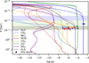 |
Fig. 13 Comparison of the cloudy+CO prior retrieval results with the VULCAN 1D photochemical kinetics model by Tsai et al. (2021) (solid lines) and thermochemical equilibrium abundances (dashed lines). The dots represent the volume mixing ratios from our retrievals (with error bars for H2O, CO2, and CO; upper limits for CH4, NH3, HCN, SO2, and H2S). The shaded regions represent the atmospheric pressure levels at which the absorption is most active for the species, starting at the cloud level at 1.44 mbar (see Fig. 11 and Table 6). For CO2 (light green) and H2O (light blue), the absorption pressure level reaches higher up in the atmosphere. The Bayesian model averaged results are similar, except for H2O, which is smaller than the VULCAN 1D results, and the CO2 abundance, which agrees with the model prediction. |
5 Discussion and conclusions
This study provides a comprehensive analysis of the atmospheric transmission spectrum of the hot Jupiter exoplanet HD 209458 b, including an updated fit to the HST/WFC3 data. To measure the abundances of line-absorbing species in the planet’s atmosphere, we performed atmospheric retrievals on the reanalysed transmission spectrum with a range of different cloud models. Using only the HST spectrum, the cloud-free model was slightly preferred. The only absorbing species conclusively detected was H2O, with a sub-solar abundance of ![Mathematical equation: $\[0.71_{-0.05}^{+0.59}\]$](/articles/aa/full_html/2025/08/aa55577-25/aa55577-25-eq77.png) × solar (Bayesian model averaged value). Although this value is low and in agreement with several previous studies (e.g. Madhusudhan et al. 2014a; Barstow et al. 2017; MacDonald & Madhusudhan 2017), the 1σ uncertainty includes the solar value. Our larger error bars are probably a better representation of the uncertainty in the cloud properties. Our approach to treat the wavelength-dependent systematics in the HST/WFC3 transmission spectrum with special attention did not change the surprisingly low water abundances measured from this spectrum. Different models without clouds yielded similar water abundances (see Table 4). Including a grey cloud deck, even if not favoured by this dataset but clearly so with the wider wavelength coverage of the added JWST/NIRCam data, pushes the water abundance to more reasonable values and probably describes the state of HD 209458 b’s atmosphere better, even if it is not statistically favoured. Accounting for the systematics in the Hubble data reduction might therefore change the abundances at a level below the current uncertainties, and other factors (e.g. the cloud coverage) have a more pronounced effect on the results. In general, our study shows that the HST/WFC3 data do not have sufficient wavelength coverage to obtain robust results for HD 209458 b.
× solar (Bayesian model averaged value). Although this value is low and in agreement with several previous studies (e.g. Madhusudhan et al. 2014a; Barstow et al. 2017; MacDonald & Madhusudhan 2017), the 1σ uncertainty includes the solar value. Our larger error bars are probably a better representation of the uncertainty in the cloud properties. Our approach to treat the wavelength-dependent systematics in the HST/WFC3 transmission spectrum with special attention did not change the surprisingly low water abundances measured from this spectrum. Different models without clouds yielded similar water abundances (see Table 4). Including a grey cloud deck, even if not favoured by this dataset but clearly so with the wider wavelength coverage of the added JWST/NIRCam data, pushes the water abundance to more reasonable values and probably describes the state of HD 209458 b’s atmosphere better, even if it is not statistically favoured. Accounting for the systematics in the Hubble data reduction might therefore change the abundances at a level below the current uncertainties, and other factors (e.g. the cloud coverage) have a more pronounced effect on the results. In general, our study shows that the HST/WFC3 data do not have sufficient wavelength coverage to obtain robust results for HD 209458 b.
We also combined our HST/WFC3 data with archival JWST/NIRCam data and retrieved the atmospheric properties based on the joint spectrum. The combined retrieval resulted in an H2O abundance of ![Mathematical equation: $\[0.95_{-0.17}^{+0.35}\]$](/articles/aa/full_html/2025/08/aa55577-25/aa55577-25-eq78.png) × solar and a CO2 abundance of
× solar and a CO2 abundance of ![Mathematical equation: $\[0.94_{-0.09}^{+0.16}\]$](/articles/aa/full_html/2025/08/aa55577-25/aa55577-25-eq79.png) × solar (with only upper limits for other species). Compared to our fits for the HST data alone, these results are in better agreement with the predictions from planet formation models and previous studies by Pinhas et al. (2019), Welbanks et al. (2019), and Welbanks & Madhusudhan (2021). To directly compare our results with the equilibrium chemistry retrieval results from Xue et al. (2024), we calculated the metallicity and C/O from the cloudy retrieval results. In our initial analysis, both values were very low ([M/H] =
× solar (with only upper limits for other species). Compared to our fits for the HST data alone, these results are in better agreement with the predictions from planet formation models and previous studies by Pinhas et al. (2019), Welbanks et al. (2019), and Welbanks & Madhusudhan (2021). To directly compare our results with the equilibrium chemistry retrieval results from Xue et al. (2024), we calculated the metallicity and C/O from the cloudy retrieval results. In our initial analysis, both values were very low ([M/H] = ![Mathematical equation: $\[-1.35_{-0.73}^{+1.25}\]$](/articles/aa/full_html/2025/08/aa55577-25/aa55577-25-eq80.png) , C/O =
, C/O = ![Mathematical equation: $\[1.33_{-0.70}^{+4.79}\]$](/articles/aa/full_html/2025/08/aa55577-25/aa55577-25-eq81.png) · 10−3), primarily due to the extremely depleted CO abundance we retrieved, which disagrees with previous ground-based high-resolution measurements of CO (Brogi & Line 2019). When we used a more informed prior on the CO abundance, based on the ground-based high-resolution results, we obtained results similar to those of Xue et al. (2024). For this case the highest likelihood model fits almost as well as the model that used a wider prior (a Bayes factor of 3 difference when the model with the wider prior is used as reference). With this result we obtained a more realistic, solar-like metallicity of [M/H] =
· 10−3), primarily due to the extremely depleted CO abundance we retrieved, which disagrees with previous ground-based high-resolution measurements of CO (Brogi & Line 2019). When we used a more informed prior on the CO abundance, based on the ground-based high-resolution results, we obtained results similar to those of Xue et al. (2024). For this case the highest likelihood model fits almost as well as the model that used a wider prior (a Bayes factor of 3 difference when the model with the wider prior is used as reference). With this result we obtained a more realistic, solar-like metallicity of [M/H] = ![Mathematical equation: $\[0.10_{-0.40}^{+0.41}\]$](/articles/aa/full_html/2025/08/aa55577-25/aa55577-25-eq82.png) and a C/O of
and a C/O of ![Mathematical equation: $\[0.054_{-0.034}^{+0.080}\]$](/articles/aa/full_html/2025/08/aa55577-25/aa55577-25-eq83.png) with a 3 σ upper limit of 0.454, which is significantly lower than the stellar C/O of 0.47 (Brewer et al. 2017).
with a 3 σ upper limit of 0.454, which is significantly lower than the stellar C/O of 0.47 (Brewer et al. 2017).
Our results highlight the sensitivity of fundamental atmospheric parameters (C/O and metallicity) to details of the model assumptions. For the HST/WFC3 data alone, we found that cloud-free models were preferred, even though clouds are strongly favoured when the JWST data are added. Similarly, even with both datasets included, CO is not detected, which tends to push the C/O and metallicity towards extremely low values. The fact that CO is not detectable in the JWST spectrum is particularly concerning, given that HD 209458 b is one of the easiest known transmission spectroscopy targets and CO is strongly detected from the ground (Brogi & Line 2019). One possible explanation is that at the low spectral resolution of these data, the carbon monoxide features are hidden by strong opacity of clouds and H2O. Another possibility is that the simplified cloud models used in the retrieval do not fully capture the effect of clouds on the spectrum. To avoid misinterpreting the spectra for this planet and others, a combination of space and high-resolution ground-based data should be considered for other studies as well. Furthermore, our analysis calls into question the use of Bayesian evidence as the sole criterion for model selection. Given that the ‘best’ models missed important features that we know to be present (cloud, CO), Bayesian model averaging is a safer approach that better captures the true model uncertainty. This is even more important for lower S/N targets, such as sub-Neptunes and Earth-like planets, where the data quality will never match what we have for a (comparatively) easy target like HD 209458 b.
To further improve our understanding of HD 209458 b’s atmosphere, future studies should consider that to get a full census of the atmospheric composition, models also need to account for species with fewer or weaker lines that are not easily visible in low-resolution transmission spectra. In general, the isothermal pressure-temperature profile and the cloud assumptions used here may also be too simplistic to fully reveal the atmospheric composition and structure of HD 209458 b. Observing the planet in the mid- to far-infrared wavelength range could provide insights into the composition of the clouds in its atmosphere. Additionally, considering different particle sizes in the clouds could offer a better understanding of their influence on the spectrum.
The low metallicity and C/O results are consistent with the picture that HD 209458 b formed by core accretion beyond and migrated inward of the snowlines of carbon-bearing species (Öberg et al. 2011), and experienced metal enrichment through pebble or planetesimal pollution before the planet reached its present-day location (Espinoza et al. 2017; Brewer et al. 2017). In general, low planetary C/O results suggest a significant amount of pebble accretion during or after the formation, and a formation further out in the protoplanetary disk where planets can accrete more icy bodies, which are in general more oxygen-rich (Cridland et al. 2019). According to Penzlin et al. (2024), very low C/O values are only reached for planets that migrated through the disc from further out, and therefore in addition accreted silicate-rich planetesimals in the inner disk where the carbon is already destroyed. These studies, together with our measured C/O result for HD 209458 b, may indicate an original formation far from its current location close to the star and strong accretion processes of solids before and during a phase of disk migration. However, these models have a number of uncertainties that make it challenging at this stage to draw firm conclusions regarding the formation of HD 209458 b (Mollière et al. 2022; Feinstein et al. 2025).
Acknowledgements
We thank the anonymous reviewer for their thorough and insightful report. This research is based on observations made with the NASA/ESA Hubble Space Telescope obtained from the Space Telescope Science Institute, which is operated by the Association of Universities for Research in Astronomy, Inc., under NASA contract NAS 5–26555. These observations are associated with programme GO 12181. This work is based in part on observations made with the NASA/ESA/CSA James Webb Space Telescope. The data were obtained from the Mikulski Archive for Space Telescopes at the Space Telescope Science Institute, which is operated by the Association of Universities for Research in Astronomy, Inc., under NASA contract NAS 5-03127 for JWST. These observations are associated with programme GTO 1274. Software used: astropy (Astropy Collaboration 2018), batman (Kreidberg 2015), ExoTiC-LD (Grant & Wakeford 2024), matplotlib (Hunter 2007), numpy (Harris et al. 2020), PACMAN (Zieba & Kreidberg 2022), petitRADTRANS (Mollière et al. 2019; Nasedkin et al. 2024a; Blain et al. 2024b), pymultinest (Buchner et al. 2014), scipy (Virtanen et al. 2020).
Appendix A Additional figures and tables
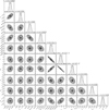 |
Fig. A.1 Corner plot with 1,2, and 3σ contours for the white light curve fit (Fig. 1), including all fit parameters. |
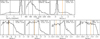 |
Fig. A.2 Bayesian model averaged results for all parameters from the model_ramp HST/WFC3 retrievals. The black line indicates the median of the distributions, and the dashed lines show the ±34.1% confidence regions. The abundances for the line-absorbing species are given in log volume mixing ratios. The orange lines indicate the solar value at 1 mbar and 1200 K. |
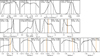 |
Fig. A.3 Averaged posterior distributions for all parameters from the combined HST-JWST retrievals using BMA. The black line indicates the median of the distributions, and the dashed lines are the ±34.1% confidence regions. The orange lines indicate the solar value at 1 mbar and 1200 K. |
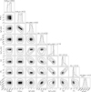 |
Fig. A.4 Corner plot for the cloudy retrieval of the joint HST-JWST spectrum, only including H2O and CO2 as line absorbers. This is the model with the highest Bayesian evidence. |
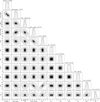 |
Fig. A.5 Corner plot for the cloudy+CO prior retrieval of the joint HST-JWST spectrum. |
Summary of retrievals run on the HST/WFC3 spectra with all the results.
Summary of retrievals run on the combined HST-JWST spectra.
Summary of retrievals run on the combined HST-JWST spectra using the more complex cloud model or a more informed prior for the CO abundance.
References
- Ahrer, E.-M., Stevenson, K. B., Mansfield, M., et al. 2023, Nature, 614, 653 [NASA ADS] [CrossRef] [Google Scholar]
- Astropy Collaboration (Price-Whelan, A. M., et al.) 2018, AJ, 156, 123 [Google Scholar]
- Azzam, A. A. A., Tennyson, J., Yurchenko, S. N., & Naumenko, O. V. 2016, MNRAS, 460, 4063 [NASA ADS] [CrossRef] [Google Scholar]
- Barstow, J. K., Aigrain, S., Irwin, P. G. J., & Sing, D. K. 2017, ApJ, 834, 50 [Google Scholar]
- Bell, T. J., Crouzet, N., Cubillos, P. E., et al. 2024, Nat. Astron., 8, 879 [Google Scholar]
- Benneke, B. 2015, arXiv e-prints [arXiv:1504.07655] [Google Scholar]
- Benneke, B., & Seager, S. 2013, ApJ, 778, 153 [Google Scholar]
- Blain, D., Landman, R., Mollière, P., & Dittmann, J. 2024a, A&A, 690, A63 [NASA ADS] [CrossRef] [EDP Sciences] [Google Scholar]
- Blain, D., Mollière, P., & Nasedkin, E. 2024b, JOSS, 9, 7028 [Google Scholar]
- Bonomo, A. S., Desidera, S., Benatti, S., et al. 2017, A&A, 602, A107 [NASA ADS] [CrossRef] [EDP Sciences] [Google Scholar]
- Booth, R. A., Clarke, C. J., Madhusudhan, N., & Ilee, J. D. 2017, MNRAS, 469, 3994 [Google Scholar]
- Brewer, J. M., Fischer, D. A., & Madhusudhan, N. 2017, AJ, 153, 83 [NASA ADS] [CrossRef] [Google Scholar]
- Brogi, M., & Line, M. R. 2019, AJ, 157, 114 [Google Scholar]
- Brogi, M., Line, M., Bean, J., Désert, J.-M., & Schwarz, H. 2017, ApJ, 839, L2 [NASA ADS] [CrossRef] [Google Scholar]
- Buchner, J., Georgakakis, A., Nandra, K., et al. 2014, A&A, 564, A125 [NASA ADS] [CrossRef] [EDP Sciences] [Google Scholar]
- Burrows, A., & Sharp, C. M. 1999, ApJ, 512, 843 [NASA ADS] [CrossRef] [Google Scholar]
- Casasayas-Barris, N., Palle, E., Stangret, M., Chen, G., & Yan, F. 2020, Eur. Planet. Sci. Cong., 811 [Google Scholar]
- Charbonneau, D., Brown, T. M., Latham, D. W., & Mayor, M. 2000, ApJ, 529, L45 [Google Scholar]
- Charbonneau, D., Brown, T. M., Noyes, R. W., & Gilliland, R. L. 2002, ApJ, 568, 377 [Google Scholar]
- Coles, P. A., Yurchenko, S. N., & Tennyson, J. 2019, MNRAS, 490, 4638 [CrossRef] [Google Scholar]
- Cridland, A. J., Dishoeck, E. F. v., Alessi, M., & Pudritz, R. E. 2019, A&A, 632, A63 [NASA ADS] [CrossRef] [EDP Sciences] [Google Scholar]
- Deming, D., Wilkins, A., McCullough, P., et al. 2013, ApJ, 774, 95 [Google Scholar]
- Dyrek, A., Min, M., Decin, L., et al. 2023, Nature, 625, 51 [Google Scholar]
- Espinoza, N., Fortney, J. J., Miguel, Y., Thorngren, D., & Murray-Clay, R. 2017, ApJ, 838, L9 [Google Scholar]
- Feinstein, A. D., Booth, R. A., Bergner, J. B., et al. 2025, ArXiv e-prints [arXiv:2506.00669] [Google Scholar]
- Foreman-Mackey, D., Hogg, D. W., Lang, D., & Goodman, J. 2013, PASP, 125, 306 [Google Scholar]
- Fortney, J. J., Mordasini, C., Nettelmann, N., et al. 2013, ApJ, 775, 80 [Google Scholar]
- Fu, G., Welbanks, L., Deming, D., et al. 2024, Nature, 632, 752 [Google Scholar]
- Giacobbe, P., Brogi, M., Gandhi, S., et al. 2021, Nature, 592, 205 [NASA ADS] [CrossRef] [Google Scholar]
- Grant, D., & Wakeford, H. R. 2024, JOSS, 9, 6816 [Google Scholar]
- Hargreaves, R. J., Gordon, I. E., Rey, M., et al. 2020, ApJS, 247, 55 [NASA ADS] [CrossRef] [Google Scholar]
- Harris, G. J., Tennyson, J., Kaminsky, B. M., Pavlenko, Y. V., & Jones, H. R. A. 2006, MNRAS, 367, 400 [Google Scholar]
- Harris, C. R., Millman, K. J., van der Walt, S. J., et al. 2020, Nature, 585, 357 [NASA ADS] [CrossRef] [Google Scholar]
- Helled, R., & Lunine, J. 2014, MNRAS, 441, 2273 [NASA ADS] [CrossRef] [Google Scholar]
- Henry, G. W., Marcy, G. W., Butler, R. P., & Vogt, S. S. 2000, ApJ, 529, L41 [Google Scholar]
- Horne, K. 1986, PASP, 98, 609 [Google Scholar]
- Hunter, J. D. 2007, Comput. Sci. Eng., 9, 90 [NASA ADS] [CrossRef] [Google Scholar]
- Kitzmann, D., Stock, J. W., & Patzer, A. B. C. 2024, MNRAS, 527, 7263 [Google Scholar]
- Kreidberg, L. 2015, PASP, 127, 1161 [Google Scholar]
- Kreidberg, L., Bean, J. L., Désert, J.-M., et al. 2014, Nature, 505, 69 [Google Scholar]
- Kurucz, R.-L. 1993, Kurucz CD-Rom, 13 (Cambridge, Mass.: Smithsonian Astrophysical Observatory) [Google Scholar]
- Leconte, J. 2021, A&A, 645, A20 [NASA ADS] [CrossRef] [EDP Sciences] [Google Scholar]
- Line, M. R., & Parmentier, V. 2016, ApJ, 820, 78 [Google Scholar]
- Line, M. R., Stevenson, K. B., Bean, J., et al. 2016, AJ, 152, 203 [NASA ADS] [CrossRef] [Google Scholar]
- MacDonald, R. J., & Madhusudhan, N. 2017, MNRAS, 469, 1979 [Google Scholar]
- Madhusudhan, N., & Seager, S. 2009, ApJ, 707, 24 [NASA ADS] [CrossRef] [Google Scholar]
- Madhusudhan, N., Crouzet, N., McCullough, P. R., Deming, D., & Hedges, C. 2014a, ApJ, 791, L9 [Google Scholar]
- Madhusudhan, N., Knutson, H., Fortney, J. J., & Barman, T. 2014b, Protostars and Planets VI, eds. H. Beuther, R. S. Klessen, C. P. Dullemond, & T. Henning (Tucson: University of Arizona Press), 739 [Google Scholar]
- Mbarek, R., & Kempton, E. M.-R. 2016, ApJ, 827, 121 [CrossRef] [Google Scholar]
- Mollière, P., Wardenier, J. P., van Boekel, R., et al. 2019, A&A, 627, A67 [Google Scholar]
- Mollière, P., Molyarova, T., Bitsch, B., et al. 2022, ApJ, 934, 74 [CrossRef] [Google Scholar]
- Nasedkin, E., Mollière, P., & Blain, D. 2024a, JOSS, 9, 5875 [Google Scholar]
- Nasedkin, E., Mollière, P., Lacour, S., et al. 2024b, A&A, 687, A298 [NASA ADS] [CrossRef] [EDP Sciences] [Google Scholar]
- Nixon, M. C., Welbanks, L., McGill, P., & Kempton, E. M.-R. 2024, ApJ, 966, 156 [Google Scholar]
- Öberg, K. I., & Bergin, E. A. 2016, ApJ, 831, L19 [Google Scholar]
- Öberg, K. I., Murray-Clay, R., & Bergin, E. A. 2011, ApJ, 743, L16 [Google Scholar]
- Penzlin, A. B. T., Booth, R. A., Kirk, J., et al. 2024, MNRAS, 535, 171 [NASA ADS] [CrossRef] [Google Scholar]
- Pinhas, A., Madhusudhan, N., Gandhi, S., & MacDonald, R. 2019, MNRAS, 482, 1485 [Google Scholar]
- Piskunov, N. E., Kupka, F., Ryabchikova, T. A., Weiss, W. W., & Jeffery, C. S. 1995, A&AS, 112, 525 [Google Scholar]
- Polyansky, O. L., Kyuberis, A. A., Zobov, N. F., et al. 2018, MNRAS, 480, 2597 [NASA ADS] [CrossRef] [Google Scholar]
- Rosenthal, L. J., Fulton, B. J., Hirsch, L. A., et al. 2021, ApJS, 255, 8 [NASA ADS] [CrossRef] [Google Scholar]
- Sing, D. K., Fortney, J. J., Nikolov, N., et al. 2016, Nature, 529, 59 [Google Scholar]
- Snellen, I. A. G., de Kok, R. J., de Mooij, E. J. W., & Albrecht, S. 2010, Nature, 465, 1049 [Google Scholar]
- Swain, M. R., Tinetti, G., Vasisht, G., et al. 2009, ApJ, 704, 1616 [Google Scholar]
- Trotta, R. 2008, Contemp. Phys., 49, 71 [Google Scholar]
- Tsai, S.-M., Malik, M., Kitzmann, D., et al. 2021, ApJ, 923, 264 [NASA ADS] [CrossRef] [Google Scholar]
- Tsai, S.-M., Lee, E. K. H., Powell, D., et al. 2023, Nature, 617, 483 [CrossRef] [Google Scholar]
- Tsiaras, A., Waldmann, I. P., Zingales, T., et al. 2018, AJ, 155, 156 [NASA ADS] [CrossRef] [Google Scholar]
- Underwood, D. S., Tennyson, J., Yurchenko, S. N., et al. 2016, MNRAS, 459, 3890 [NASA ADS] [CrossRef] [Google Scholar]
- Verma, A., Goyal, J., Avarsekar, S., & Shukla, G. 2025, arXiv e-prints [arXiv:2505.04413] [Google Scholar]
- Virtanen, P., Gommers, R., Oliphant, T. E., et al. 2020, Nat. Methods, 17, 261 [Google Scholar]
- Welbanks, L., & Madhusudhan, N. 2021, ApJ, 913, 114 [NASA ADS] [CrossRef] [Google Scholar]
- Welbanks, L., Madhusudhan, N., Allard, N. F., et al. 2019, ApJ, 887, L20 [NASA ADS] [CrossRef] [Google Scholar]
- Woitke, P., Helling, C., Hunter, G. H., et al. 2018, A&A, 614, A1 [NASA ADS] [CrossRef] [EDP Sciences] [Google Scholar]
- Xue, Q., Bean, J. L., Zhang, M., et al. 2024, ApJ, 963, L5 [NASA ADS] [CrossRef] [Google Scholar]
- Yurchenko, S. N., Mellor, T. M., Freedman, R. S., & Tennyson, J. 2020, MNRAS, 496, 5282 [NASA ADS] [CrossRef] [Google Scholar]
- Zieba, S., & Kreidberg, L. 2022, JOSS, 7, 4838 [Google Scholar]
https://simbad.cds.unistra.fr/simbad/sim-id?Ident=HD+209458, 15.11.2023.
All Tables
Parameters for the spectroscopic light curve fits with assigned uniform priors (U).
Summary of retrievals run on the combined HST-JWST spectra using the more complex cloud model or a more informed prior for the CO abundance.
All Figures
|
Fig. 1 White light curve of HD 209458 b’s HST/WFC3 transit with the best-fit transit model (upper left panel) and residuals of the fit (upper right panel), as well as the spectral light curves (lower left panel; offset) with fit transit models and the corresponding residuals (lower right panel). |
| In the text | |
|
Fig. 2 Variation in the fitted model_ramp parameters r1 and r2 (cf. Eq. (1)) with wavelength. The dots represent best-fit values in each wavelength bin with 1 σ errors from the posterior. Both r1 and r2 are clearly not wavelength-independent. |
| In the text | |
|
Fig. 3 Comparison of HST/WFC3 transmission spectra with (blue) and without (green) applying the additional Gaussian convolution (see Sect. 2.2) in the data reduction. Both spectra use the model_ramp model. The green spectrum without the additional smoothing step shows a zig-zag pattern of alternating transit depths between subsequent exposures. The grey spectrum is from Deming et al. (2013) for comparison. |
| In the text | |
|
Fig. 4 Comparison of HST/WFC3 transmission spectra for three different data reduction and fitting methods for HD 209458 b. The blue spectrum uses exponential functions to fit the systematics at the beginning of each orbit (model_ramp fit), whereas the green spectrum assumes wavelength independent systematics (divide_white fit). The grey spectrum is the original transmission spectrum published by Deming et al. (2013). The right panels show the differences between all three spectra. Noticeable is the linear trend with wavelength in the residuals for all three cases. |
| In the text | |
|
Fig. 5 Comparison of best-fit spectra with different cloud assumptions. The retrieval uses the model_ramp fit HST/WFC3 spectrum (grey dots). All three retrievals include all tested absorbing species (see Table 4). The red spectrum is cloud-free, the blue one cloudy, and the orange spectrum is the best fit for patchy clouds. |
| In the text | |
|
Fig. 6 Comparison of best-fit cloud-free spectra for retrievals of the model_ramp fit HST/WFC3 spectrum. The red spectrum is the same as in Fig. 5. The orange spectrum is the best fit for the model with the highest Bayesian evidence (clear atmosphere and only H2O as line absorber). The light blue spectrum is the model that does not contain water as an absorber. |
| In the text | |
|
Fig. 7 Bayesian model averaged posterior distribution for H2O from the HST/WFC3 retrievals. The black line indicates the median of the distribution, and the dashed lines are the ±34.1% confidence regions. The orange lines shows the solar value (log(χH2O) = −3.70) at 1 mbar and 1200 K. Since most of the models used for the BMA do not include clouds, the results are more heavily weighted towards the cloud-free solution, and therefore lower H2O abundances (see text). |
| In the text | |
|
Fig. 8 Comparison of best-fit spectra for retrievals of the joint HST-JWST spectrum using different cloud models. The fits include all tested absorbing species except for SO2 and H2S (see Table 6). The red spectrum is cloud-free, the blue spectrum is cloudy, and the orange spectrum is the best fit for patchy clouds. The dashed spectra are the best fits using the more complex cloud model described in Sect. 4.3. We also fit for an offset between the HST and JWST data, which is visible by eye in the figure (for details, see Tables A.2 and A.3). |
| In the text | |
|
Fig. 9 Comparison of best-fit spectra for retrievals of the joint HST-JWST spectrum using different molecular absorbers and a grey cloud. The orange spectrum is the best-fit case from the model with the highest Bayesian evidence: a grey cloud and only H2O and CO2 as line absorbers. The light blue dashed spectrum does not include water as an absorber, whereas the light green dashed spectrum is without CO2. The dark green spectrum is the best fit of the cloudy+CO prior model (see Sect. 4.5). As in Fig. 8, there is a vertical offset between the HST and JWST data. |
| In the text | |
|
Fig. 10 Bayesian model averaged posterior distributions for H2O (left) and CO2 (right). The black line indicates the median of the distributions, and the dashed lines are the ±34.1% confidence regions. The orange lines show the solar value of log(χH2O) = −3.70 and log(χCO2) = −7.05 at 1 mbar and 1200 K. |
| In the text | |
|
Fig. 11 Contribution of the opacities of line-absorbing species to the transmission spectrum. The best-fit spectrum shows the cloudy+CO prior model (see text). The absorption features of H2O and CO2 are clearly visible, for the latter due to its strong absorption even though the abundance is low (see Fig. 10). |
| In the text | |
|
Fig. 12 Metallicity (left) and C/O (right) distribution calculated from the posterior distributions of the cloudy+CO prior retrieval. The black solid lines indicate the median, and the dashed lines depict the ±34.1% confidence regions. The dotted line shows the 3σ upper limit of 0.454 for C/O. The same calculations without a tight CO prior yielded a very sub-solar metallicity of [M/H] = |
| In the text | |
|
Fig. 13 Comparison of the cloudy+CO prior retrieval results with the VULCAN 1D photochemical kinetics model by Tsai et al. (2021) (solid lines) and thermochemical equilibrium abundances (dashed lines). The dots represent the volume mixing ratios from our retrievals (with error bars for H2O, CO2, and CO; upper limits for CH4, NH3, HCN, SO2, and H2S). The shaded regions represent the atmospheric pressure levels at which the absorption is most active for the species, starting at the cloud level at 1.44 mbar (see Fig. 11 and Table 6). For CO2 (light green) and H2O (light blue), the absorption pressure level reaches higher up in the atmosphere. The Bayesian model averaged results are similar, except for H2O, which is smaller than the VULCAN 1D results, and the CO2 abundance, which agrees with the model prediction. |
| In the text | |
|
Fig. A.1 Corner plot with 1,2, and 3σ contours for the white light curve fit (Fig. 1), including all fit parameters. |
| In the text | |
|
Fig. A.2 Bayesian model averaged results for all parameters from the model_ramp HST/WFC3 retrievals. The black line indicates the median of the distributions, and the dashed lines show the ±34.1% confidence regions. The abundances for the line-absorbing species are given in log volume mixing ratios. The orange lines indicate the solar value at 1 mbar and 1200 K. |
| In the text | |
|
Fig. A.3 Averaged posterior distributions for all parameters from the combined HST-JWST retrievals using BMA. The black line indicates the median of the distributions, and the dashed lines are the ±34.1% confidence regions. The orange lines indicate the solar value at 1 mbar and 1200 K. |
| In the text | |
|
Fig. A.4 Corner plot for the cloudy retrieval of the joint HST-JWST spectrum, only including H2O and CO2 as line absorbers. This is the model with the highest Bayesian evidence. |
| In the text | |
|
Fig. A.5 Corner plot for the cloudy+CO prior retrieval of the joint HST-JWST spectrum. |
| In the text | |
Current usage metrics show cumulative count of Article Views (full-text article views including HTML views, PDF and ePub downloads, according to the available data) and Abstracts Views on Vision4Press platform.
Data correspond to usage on the plateform after 2015. The current usage metrics is available 48-96 hours after online publication and is updated daily on week days.
Initial download of the metrics may take a while.