| Issue |
A&A
Volume 700, August 2025
|
|
|---|---|---|
| Article Number | A195 | |
| Number of page(s) | 19 | |
| Section | Catalogs and data | |
| DOI | https://doi.org/10.1051/0004-6361/202555695 | |
| Published online | 19 August 2025 | |
Survey of Surveys
II. Stellar parameters for 23 million stars
1
INAF – Osservatorio Astrofisico di Arcetri,
Largo E. Fermi 5,
50125
Firenze,
Italy
2
Space Science Data Center,
Via del Politecnico SNC,
00133
Roma,
Italy
3
INAF – Osservatorio Astronomico di Roma,
Via Frascati 33,
00040,
Monte Porzio Catone, Roma,
Italy
4
Institute of Astronomy,
48 Pyatnitskaya St.,
119017
Moscow,
Russia
5
Dipartimento di Fisica e Astronomia, Università di Firenze,
Via G. Sansone 1,
50019
Sesto Fiorentino,
FI,
Italy
6
Instituto de Astrofísica de Canarias,
38205
La Laguna,
Tenerife,
Spain
7
Universidad de La Laguna, Dpto. Astrofísica,
38206
La Laguna,
Tenerife,
Spain
8
Université Côte d’Azur, Observatoire de la Côte d’Azur, CNRS, Laboratoire Lagrange,
Nice,
France
9
Zentrum für Astronomie der Universität Heidelberg, Landessternwarte,
Königstuhl 12,
69117
Heidelberg,
Germany
10
Max Planck Institute for Astronomy,
Königstuhl 17,
69117
Heidelberg,
Germany
11
Leibniz-Institut für Astrophysik Potsdam (AIP),
An der Sternwarte 16,
14482
Potsdam,
Germany
★ Corresponding author.
Received:
28
May
2025
Accepted:
2
July
2025
Abstract
Context. In the current panorama of large surveys, the vast amount of data that are obtained with different methods, data types, formats, and stellar samples prevents an efficient use of the available information.
Aims. The Survey of Surveys is a project to critically compile survey results into a single catalog to facilitate the scientific use of the available information. In this second release, we present two new catalogs of stellar parameters (Teff, log g, and [Fe/H]).
Methods. To build the first catalog, SoS-Spectro, we internally and externally calibrated stellar parameters from five spectroscopic surveys (APOGEE, GALAH, Gaia-ESO, RAVE, and LAMOST). Our external calibration on the PASTEL database of high-resolution spectroscopy ensures better performances for data of metal-poor red giants. The second catalog, SoS-ML catalog, is obtained by using SoS-Spectro as a reference to train a multilayer perceptron that predicts stellar parameters based on two photometric surveys, SDSS and SkyMapper. As a novel approach, we built on previous parameter sets from Gaia DR3 and other sources to improve their precision and accuracy.
Results. We obtained a catalog of stellar parameters for about 23 million stars that we make publicly available. We validated our results with several comparisons with other machine-learning catalogs, stellar clusters, and astroseismic samples. We found substantial improvements in the parameter estimates compared to other machine-learning methods in terms of precision and accuracy, especially in the metal-poor range. This was particularly evident when we validated our results with globular clusters.
Conclusions. Our results at the low-metallicity end improve for two reasons: First, we used a reference catalog (the SoS-Spectro) that was calibrated using high-resolution spectroscopic data; and second, we chose to build on pre-existing parameter estimates from Gaia and Andrae et al. and did not attempt to obtain our predictions from survey data alone.
Key words: methods: data analysis / methods: numerical / techniques: spectroscopic / catalogs / surveys / stars: fundamental parameters
© The Authors 2025
 Open Access article, published by EDP Sciences, under the terms of the Creative Commons Attribution License (https://creativecommons.org/licenses/by/4.0), which permits unrestricted use, distribution, and reproduction in any medium, provided the original work is properly cited.
This article is published in open access under the Subscribe to Open model. This email address is being protected from spambots. You need JavaScript enabled to view it. to support open access publication.
1 Introduction
Large-scale spectroscopic surveys have significantly advanced our understanding of stellar astrophysics by providing a tremendous amount of spectra for several million stars, including spectra with a low to medium resolution, such as those from the RAdial Velocity Experiment (RAVE; Steinmetz et al. 2006), the Sloan Extension for Galactic Understanding and Exploration (SEGUE; Yanny et al. 2009), and the Large sky Area Multi Object fiber Spectroscopic Telescope (LAMOST; Zhao et al. 2012), or spectra at high resolution, such as the Galactic Archaeology with HERMES (GALAH; Buder et al. 2018), the Apache Point Observatory Galactic Evolution Experiment (APOGEE; Schiavon et al. 2024), and the Gaia-ESO survey (Gilmore et al. 2012). The data provided by these surveys allow us to directly derive precise estimates of key parameters such as the effective temperature (Teff), the surface gravity (log ɡ), the metallicity ([Fe/H]), and individual chemical abundances for a few million stars in the Milky Way.
In recent years, these surveys spawned several works that were focused on machine-learning (ML) methods (i.e., neural networks or simpler methods) in order to extract information from stellar spectra (Ness et al. (2015); Ting et al. (2019); Fabbro et al. (2018); Guiglion et al. (2024); Anders et al. (2022)). ML in astrophysics saw a huge development in the last decades of the twentieth century and rose to a widespread usage in the first decades of the twentyfirst century. The term can be used in general to cover different disciplines from artificial intelligence to neural networks and computational statistics. In general, we refer to ML techniques when we speak of algorithms that make use of heterogeneous or generally complex data to automatically learn and build a model that produces a desired output with statistical methods.
High-quality spectroscopic measurements are hard to obtain on large stellar samples, however, which require much telescope time, and thus, most of the available data come from photometric surveys, which provide observations in many different bands that include hundreds of millions (up to billions) of stars. Some of the most important photometric surveys are the Sloan Digital Sky Survey (SDSS; Abazajian et al. 2003), the SkyMapper Southern Sky Survey (SM; Keller et al. 2007), and the Two Micron All-Sky Survey (2MASS; Skrutskie et al. 2006). While not as accurate as spectroscopic data, photometry can indeed be used to derive a rough estimate of Teff, log ɡ, and [Fe/H], mainly by employing empirical or theoretical relations, and it is used by many astronomers to analyze huge star samples. The availability of high-quality spectroscopic measurements, together with reliable estimates of distance and reddening, is of paramount importance to derive high-quality estimates of the above parameters from photometric surveys.
With this in mind, we provide here the second data release of the Survey of Surveys, which presents astrophysical parameters for about 23 million stars. It contains (i) a new version of the spectroscopic Survey of Surveys (SoS-Spectro, see Tsantaki et al. 2022) and (ii) the first version of the Survey of Suveys obtained with ML (SoS-ML). In particular, we calibrate the SoS-Spectro parameters with external high-resolution spectro-scopic parameters. For SoS-ML, we obtain stellar parameters from photometric surveys by improving the accuracy compared to literature ML estimates, or in other words, by enhancing previous estimates. The strength of this method is that unlike in purely predictive approaches (without initial estimates in the input features), we did not try to produce parameter estimates from scratch and are therefore less affected by strong deviations of the model from the real measurement. To achieve this goal and train our ML model, we used the spectroscopic estimates of Teff, log ɡ, and [Fe/H] provided by SoS-Spectro. We also used the astrometric, photometric, and spectroscopic data from Gaia DR3 to obtain parameters based on large photometric datasets such as SM for the southern and SDSS for the northern hemisphere.
This paper is organized as follows: in Sect. 2 we describe our selected data samples from Gaia DR3, SDSS, and SM. In Sect. 3, we calibrate the reference SoS-Spectro catalog. In Sect. 4, we describe the algorithm we used and its training. In Sect. 5, we build the SoS-ML catalog. In Sect. 6, we validate the results, and in Sect. 7, we summarize our results and draw our conclusions.
2 Reference datasets
Our analysis is based on different data sources. We describe the selection and preparation of the catalogs for each of the sources below.
2.1 Gaia
Gaia DR3 data1 (Gaia Collaboration 2023) were used to facilitate an accurate cross-match between catalogs. In particular, the coordinates reported in our final catalog are in the Gaia DR3 system. We also used several indicators of stellar blending, binarity, nonstellarity, and variability to clean the sample.
Part of the information in the Gaia catalog, such as magnitude, colors, and stellar parameters, were used as input parameters for our work. We complemented the Gaia DR3 catalog with distances derived by Bailer-Jones et al. (2021). Finally, we used teff_gspphot and logg_gspphot as input parameters (Sect 4.2); we used the [Fe/H] estimates from Andrae et al. (2023) instead of mh_gspphot from Gaia DR3 because we realized that they agree with the SoS-Spectro metallicities better than those of Gaia. Specifically, we observed an overall Root Mean Square Error (RMSE) that is better by 0.15 dex on the whole sample and 0.22 dex better on low-metallicity stars ([Fe/H] ≤ −1.5 dex). Because our goal is to estimate the SoS-Spectro measurements, this difference had a definitely positive impact.
We applied the following selection criteria:
We removed sources without either phot_bp_mean_mag or phot_rp_mean_mag.
We removed sources with ipd_frac_multi_peak> 10, ipd_frac_ odd_win > 10, or ruwe > 1.4 to avoid contamination by neighboring objects (see also Lindegren et al. 2021; Mannucci et al. 2022);.
We removed sources with the non_single_star or VARIABLE flags and those with the in_qso_candidates and in_galaxy_candidates flags.
We only included sources with a distance in Bailer-Jones et al. (2021) and in particular used the geometric distance determinations because we noted a posteriori that they produced slightly better results.
We removed stars with a spectroscopic rotational broadening (vbroad) of more than 30km s−1 when this parameter was available because their colors might be altered by gravity darkening and their spectroscopic parameters are less reliable.
We removed all stars with a photometric temperature (teff_gspphot) greater than 9000 K because they were not consistent among the spectroscopic surveys.
We removed stars with G > 18 mag, parallax_error > 0.1 or astrometric_sigma5d_max> 0.1 because their astro-metric parameters were worse. After initial tests, we realized that ≃13% of the stars were clearly giants in the spectroscopic surveys, but they lay on the main sequence in the absolute and dereddened Gaia color-magnitude diagram. This conflicting information confused the algorithm so that it provided incorrect log ɡ predictions for many stars in the training set. The adopted cut reduced the stars with conflicting information to about 1% of the global sample and significantly improved our predictions.
2.2 SDSS
For the northern hemisphere, we used photometry from SDSS DR132 (Albareti et al. 2017). In DR13, no new data were added, but the previous SDSS photometric data were recalibrated and thus improved considerably. The release contains almost half a billion objects with five-band uɡriɀ photometry (Fig. 1). We cross-matched SDSS with our Gaia DR3 selected sample (Sect. 2.1) using the software by Marrese et al. (2017, 2019). We dropped all stars in each catalog that corresponded to more than one star in the other catalog. This selection might appear very strict, but for this initial experiment, we preferred to work on the cleanest possible sample of stars.
We removed galaxies from SDSS DR13 with type=6, and we used only well-measured stars with clean=1. To facilitate the cross-match with Gaia, we also removed stars with any of the five uɡriɀ magnitudes outside of the range 0–25 mag. We excluded stars with fewer than two valid magnitude measurements and stars with reddening greater than 10 mag in the ɡ band. After these selections and after cross-matching with our cleaned sample from Gaia DR3, our SDSS dataset contained about nine million stars that are distributed in the sky as shown in Fig. 2.
We computed the absolute magnitudes using Gaia distances D (Bailer-Jones et al. 2021) and the extinction coefficients AB from the SDSS catalog in each band B using the equation
 (1)
(1)
where MB and mB are the absolute and relative magnitudes in each band B, respectively. We used the absorption coefficients AB that are provided in the SDSS catalog for each band.
 |
Fig. 1 Photometric passbands of Gaia (top panel), SDSS (middle panel), and SkyMapper (bottom panel) as obtained from the SVO filter profile service (Rodrigo et al. 2024, http://svo2.cab.inta-csic.es/theory/fps/). |
2.3 Skymapper
For the southern hemisphere, we relied on SkyMapper DR23 (Huang et al. 2021), which contains photometry in the six uvgriz bands (Fig. 1) for half a billion stars. We cross-matched SM with our selection of sources from Gaia DR3 using the software by Marrese et al. (2017, 2019), and similarly to the case of the SDSS, we removed from each catalog all stars that corresponded to more than one star in the other catalog. We computed absolute magnitudes as in the case of SDSS (Eq. (1)). We used E(B−V) provided in the SM catalog, which was obtained from the maps by Schlegel et al. (1998), and we obtained the AB absorption in each band B following the SM recipes4. We removed stars with reddening greater than 10 mag in the ɡ band. To remove most nonstellar objects, we used the criterion classStar >0.8. We also removed problematic measurements with the conditions flag=0 and flagPSF=0. Similarly to the SDSS case, we removed stars outside the range 0–25 mag. After these selections and after cross-matching with our cleaned Gaia DR3 sample, the sample contained ten million stars that are distributed in the sky as shown in Fig. 2.
3 Spectroscopic Survey of Surveys
Our sample of stars with known spectroscopic Teff, log ɡ, and [Fe/H] (which we used as labels, according to the ML conventions) was obtained from the first SoS data release (Tsantaki et al. 2022)5. Although the release only contains radial velocities (RV), a preliminary catalog of stellar parameters was also prepared (hereafter SoS-Spectro) and used to study the trend of RV in each survey against different parameters. This was built using the following spectroscopic surveys: APOGEE DR16 (Ahumada et al. 2020), GALAH DR2 (Buder et al. 2018), Gaia-ESO DR3 (Gilmore et al. 2012), RAVE DR6 (Steinmetz et al. 2020a,b), and LAMOST DR5 (Deng et al. 2012). The homogenization procedure was very simple (see equations in Appendix A by Tsantaki et al. 2022): The Teff of LAMOST and the [Fe/H] of RAVE were calibrated, and then an average of all surveys was taken. The typical uncertainties of SoS-Spectro are nevertheless quite small, about ≲100 K in Teff and ≃0.1 dex in log ɡ and [Fe/H], and the catalog contains almost five million stars.
SoS-Spectro was already successfully used to characterize the Landolt and Stetson secondary standard stars (Pancino et al. 2022), with excellent results even for difficult parameters such as low log ɡ or [Fe/H]. The final SoS-Spectro parameters, homogenized and recalibrated as described below, are made available along with those derived from the SDSS and SM photometry using ML (see Sect. 5). The few duplicates that were present in the original SoS preliminary catalog were removed and were not considered in this study.
3.1 External calibration of SoS-Spectro
Before we proceeded, we compared the SoS-Spectro parameters with a high-resolution compilation from the literature, the PASTEL database (Soubiran et al. 2016). The resulting median and median absolute deviations (hereafter MAD6) for SoS-Spectro minus PASTEL are ∆Teff = −9 ± 143 K, ∆log ɡ = −0.05 ± 0.21 dex, and ∆[Fe/H]=0 ± 0.11 dex. This is quite satisfactory. A large spread and overestimation are present in the log ɡ comparison for giants (up to 2 dex), which appears to worsen at lower metallicity. We verified that the same behavior appears in the individual surveys when compared with PASTEL (see also Figs. 3 to 8 by Soubiran et al. 2022), and therefore, it is not a result of our recalibration and merging procedure, but is a consistent and systematic difference between PASTEL and each of the considered spectroscopic surveys. We suspect that the problem might be related to the practical difficulties of measuring correct abundances for metal-poor giants, but based on this comparison, it is difficult to decide whether the problem lies in PASTEL or in the surveys. We also observe that above ≃7000 K, the Teff agreement between PASTEL and SoS-Spectro breaks down. The reason is that the spectroscopic surveys disagree in general with each other in this temperature regime. Therefore, we expect the agreement to improve when we apply a more sophisticated homogenization and external recalibration procedure in future releases of the SoS-Spectro catalog.
We also compared our [Fe/H] results with data from open and globular clusters (see also Sect. 6.4) and observed the same trend as in the PASTEL comparison. Based on this, we decided to calibrate our SoS-Spectro results against PASTEL using a three-parameter linear fit. We fit the difference SoS-Spectro minus PASTEL with the following function:
![Mathematical equation: $\Delta f = a + b \cdot {\rm{T}}_{{\rm{eff}}}^{{\rm{SoS}}} + {\rm{c}} \cdot {\rm{log}}\,{{\rm{g}}^{{\rm{SoS}}}} + {\rm{d}} \cdot {\left[ {{\rm{Fe/H}}} \right]^{{\rm{SoS}}}}.$](/articles/aa/full_html/2025/08/aa55695-25/aa55695-25-eq2.png) (2)
(2)
This fit was computed for ≃15 000 measurements, corresponding to ≃14000 unique stars in common. In Fig. 3 we show the result of this correction. On average, the computed error correction values are −36.8 K for Teff, 0.05 dex for log ɡ, and −0.008 dex for [Fe/H]. The fit correction coefficients for Teff, log ɡ, and [Fe/H] are summarized in Table 1. The deviations at low log ɡ and [Fe/H] were more than halved after the recalibration on PASTEL.
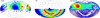 |
Fig. 2 Sky distribution of our sample selections after the cross-match with Gaia and all quality selections (Sect. 2) in an Aitoff projection of RA and Dec. The color scale refers to the density of points (blue is the minimum density, and red is the maximum density). |
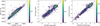 |
Fig. 3 Comparison of the SoS-Spectro atmospheric parameters (Tsantaki et al. 2022, after calibration) with the literature compilation of high-resolution studies in the PASTEL database (Soubiran et al. 2016), for ≃15 000 measurements, corresponding to ≃14 000 unique stars in common (see Sect. 3 for details). The lighter color corresponds to a higher data density per pixel. The gray points in the background represent the uncorrected data before we applied Eq. (2). |
3.2 Systematics due to survey releases in SoS-Spectro
It is important to note that the SoS-Spectro parameters we present are not based on the latest releases of spectroscopic surveys and Gaia. The latest releases contain several improvements in the data analysis pipelines that are expected to yield more accurate spectroscopic parameters. Preliminary tests revealed some biases in the SoS-Spectro parameters, in particular, when plotted against the absolute G-band magnitude. These biases are attributed to differences in the data releases of individual surveys (see Appendix A), with observed oscillations as a function of absolute magnitude in the following ranges: about 10–150 K in Teff, 0.1–0.3 dex in log ɡ, and 0.02–0.15 dex in [Fe/H] (see Fig. A.1).
Fit correction coefficients for Teff, log ɡ, and [Fe/H].
4 Neural network model
In our previous work (Pancino et al. 2022), we applied a few simple ML algorithms (i.e., random forest, K-neighbors, and support vector regression, or SVR) to a sample of about 6000 secondary standard stars from Landolt and Stetson photometry, with excellent results. In this study, however, the sample size is larger by a few orders of magnitude, and we immediately realized that even the simplest multilayer perceptron (MLP) network quickly outperformed other simpler ML techniques such as SVR.
The nonlinear technique MLP uses artificial neurons and is thus often called artificial neural network (ANN). The neurons each have an activation function that depends on an input. A matrix of neurons defines a layer, and multiple layers can be stacked (the output of each layer serves as the input to the next layer). Each neuron is connected with all the inputs, and specific weights determine which input and how an input contributes to activating the neuron itself to produce an output, based on a nonlinear activation function. Training is performed on a dataset sample in order to converge the weights to the optimal numbers that best reduces the error on the output, using what is generically called a loss function (i.e., the mean error, RMSE, and so on). MLP usually performs better the larger the training dataset, but it is harder to interpret than simpler methods.
4.1 Network design
We used the Keras Python interface (Chollet et al. 2015) for the TensorFlow library (Abadi et al. 2015). The MLP network was built by sequentially stacking a fully connected (dense) layer with a leaky rectified linear unit activation function (leaky ReLU), a batch normalization layer, and a dropout layer7. The batch normalization layer maintains the mean output close to zero with a standard deviation equal to one. The leaky ReLU was chosen because the network performs and converges better. The leaky ReLU together with normalization helped us to compensate for the vanishing-gradient problem, where some coefficient continuously decreases with the depth of the network, and eventually impairs the ability to efficiently use all layers to learn from input. Both batch normalization and dropout layers helped us to avoid overfitting (i.e., a poorly generalized solution).
We selected a total of 18 hidden layers with varying sizes between 80 and 160 elements, with the smaller sizes at the extremes and the larger sizes in the middle (i.e., a diamond shape). During the training, we varied the loss function by allowing the model to minimize the mean absolute error for the first 20% of training time. During the remaining 80% of the training time, the model instead minimized the symmetric mean absolute percentage error (SMAPE), which is defined as
 (3)
(3)
where y is the true (reference) value, ypred is the value predicted by the network, and ϵ = 10−3 is a low value introduced in order to avoid an explosion of the function. This choice allowed us to optimize the convergence by first reducing the maximum error over the whole dataset, thus trying to minimize the effect of outliers, and finally, to reduce the relative error in a second phase.
For each required output parameter (Teff, log ɡ, and [Fe/H]), we trained a different network for performance reasons on limited hardware. The output layer therefore is only one element wide. In the future, we will experiment with more complex methods that also exploit the interdependence of the three parameters, but the current results are satisfactory (see also Sect. 6).
Other precautions were taken in order to allow the network to provide a robust response even when some of the input parameters were missing. Specifically, we added a flag for each parameter (thus doubling the input size) that takes a boolean value to indicate the presence of a valid measure for the corresponding parameter. Then, we proceeded to substitute all missing parameters with zeros, which allowed the network to operate even in the presence of missing values. Since the network knows whether a measure is available, it can take this information into account when it processes the input and can produce an output even when data are missing. This is a common occurrence in large and heterogeneous catalogs.
4.2 Choice of input parameters (features)
The final choice of the input parameters (called “features” in the ML lexicon) was made following two different strategies. On the one hand, we tried a brute-force approach by adding as many input parameters as possible and discarding only those that were clearly irrelevant (e.g., source IDs). On the other hand, we selected a list of parameters that are commonly considered relevant from the astrophysical point of view for predicting the quantities of interest (e.g., dereddened colors, to predict the temperature). We finally followed an intermediate approach by adding those parameters to the physically relevant list of parameters that in the brute-force list appeared to improve the result by reducing the error of one percent at least. We also removed some of the apparently relevant parameters that appeared to provide a negligible contribution to the final accuracy to reduce computing times.
In Tables 2 and 3, we report the selected input parameter lists for the SDSS and SM samples, respectively. They differ slightly mainly because the υ band was added in SM. For each band, we included both the reddened and dereddened absolute magnitudes because we realized that the two most important parameters for our algorithm were distance and reddening. Since reddening can sometimes be very high (we obtained values up to 500 in ɡ band for a few stars before the filtering), we observed a small but consistent increase in the performance (around 10%) when the dereddened magnitudes were added, perhaps because the algorithm can take reddening deviations better into account and computes the prediction accordingly. The parameter selection in Sect. 2 means that the applicability of the ML method we discuss is limited by the same constraints. This means that we only applied the method for input parameters that satisfied a certain quality standard.
Because of the typical problems that are encountered in massive ML predictions of astrophysical parameters and in spectroscopic surveys, which normally concern metal-poor stars and red giants or hot stars, we decided to test a different approach. We therefore also added estimates of Teff, log ɡ, from Gala DR3, and [Fe/H] from Andrae et al. (2023, see also Sect. 2.1) to the list of input parameters because our preliminary tests showed that the algorithm would benefit from an initial estimate. As we show in Section 6, this also allowed us to improve the predictions compared to that initial estimate. We also realized that adding the error estimates for the same parameters consistently increased the performance by a few percent, probably because the errors helped the algorithm to determine how much trust to place in each provided estimate.
4.3 Training and testing
We cross-matched our previously selected SDSS and SM samples with SoS-Spectro and obtained two different samples of about 300 000 and 800 000 stars, respectively. These samples provided the spectroscopic measurements for Teff, log g, and [Fe/H] that we used as labels to train the model. In our first attempts, we observed that our model performed poorly (with an evident overestimation) on very low metallicities ([Fe/H] ≲ −2 dex) because the two training samples had very few stars in that metallicity range. This is a common problem for spectro-scopic surveys and ML methods (see Sect. C.1 and Fig. C.1). We thus added metal-poor stars from the PASTEL catalog to the SoS sample because they agree well with the recalibrated SoS-Spectro. We selected stars with [Fe/H] < −1 dex in common with the SDSS and SM samples, which yielded an additional 139 and 267 stars, respectively. While the numbers may seem small, they increased the population of very metal-poor stars by an order of magnitude. As detailed in Appendix C.1, the addition of these very metal-poor stars did not solve the problem of spec-troscopic surveys and ML methods in this metallicity range, but it did improve the [Fe/H] performance over the entire metallicity range (Fig. C.1).
On the previously defined SDSS and SM training samples, where we had the SoS (and very few PASTEL) measurements for Teff, log ɡ, and [Fe/H] to act as a label, we trained two different networks and reserved 80% of the sample for the training phase, 10% for the internal validation phase, and 10% for the final testing phase. We monitored that the performance on the testing sample was never too far from the performance obtained on the training and validation samples in order to avoid overfitting.
In principle, the reference dataset, SoS-Spectro, is the true measure that we wish to reproduce. It is clear, however (Sects. 3.1 and 6), that the reference catalog itself has its own random deviations and biases, which will be faithfully reproduced by the MLP. In other words, the algorithm cannot perform better than the reference dataset. Therefore, any error estimate on the MLP performance needs to be combined with the uncertainties in the reference dataset (see Sect. 5.1). In Fig. 4, we show the MLP error distribution obtained on the test subsample (without any other error contribution, i.e., the difference with respect to SoS-Spectro).
In order to characterize the model performance, we report various error determinations in Table 4. The results for the SDSS and SM only show modest biases of ≃50 K in Teff, ≃0.1 dex in log ɡ, and a bias lower than 0.1 dex in [Fe/H]. The mean and the σ are slightly higher than the median and the MAD because of a long tail of rare, but high errors, as shown in Fig. 4.
In Figure 5, we show the comparison between the ML predictions on the stars in common between the SM and SDSS training and test datasets (55 696 stars). The models used for each set came from a different training on slightly different parameters, and the excellent agreement between the two predictions therefore is proof that the method is robust enough to be trusted preliminarily. We find median differences of 26 K in Teff, 0.03 dex in log ɡ, and 0.04 dex in [Fe/H].
Errors of the ML-predicted variables on the test sample with respect to errors from SoS-Spectro.
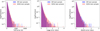 |
Fig. 4 Distribution of the ML prediction errors on the test dataset in the SM (blue) and SDSS sample case (red). The y-scale indicates the logarithm of the fraction of the training dataset in each bin (a total of 100 bins). |
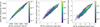 |
Fig. 5 Comparison between the ML predictions obtained on the intersection between SDSS and SM training plus test sample and SM sample (55 696 stars). The lighter color corresponds to a higher data density per pixel. |
5 Machine-learning Survey of Surveys
After validating the performance of the method on the test sample, we ran the trained model on the full datasets of the SM and SDSS (i.e., not just the stars that were matched against SoS-Spectro). Each dataset accounts for about nine to ten million stars after the relevant filtering was applied (see Sects. 2.2 and 2.3).
5.1 Error estimation
In Table 4, we reported the median error obtained on the test subsample by comparing the ML-predicted values with the reference values of SoS-Spectro. In the following, we will refer to this error component as etrain. It represents the accuracy of the ML method.
In order to test the repeatability of the model predictions against the choice of the training sample, we realized ten different trainings of the model for each of the SDSS and SM datasets, starting from different random choices of the training, validation, and test samples. For each parameter, we then computed the MAD of the predictions for each star in the full set, obtained with the ten differently trained models, along with the median prediction. We used our median prediction as our actual prediction and thus mitigated the impact of potential random outliers, and we used the MAD as a repeatability (precision) error component that we hereafter refer to as erep.
Our final error estimate for each parameter and each star in the SM and SDSS datasets is the result of the combination of the two previously identified error components (etrain and erep), which are considered independent and thus summed in quadrature,
 (4)
(4)
This error was included in the final catalog (Sect. 5.2). In Table 5 we report its mean and median value for each parameter and each dataset. The Kiel diagrams of the two sets of predictions for the SDSS and SM datasets, colored by the estimated errors, are shown and discussed in Appendix B, together with the respective error distributions.
5.2 Final catalog
To compose the final catalog of ML-predicted parameters, we merged the SM and SDSS datasets by averaging the predictions obtained on stars in common, which are compatible with each other (see Fig. 5). We applied the following filters on the final ML-predicted parameters and errors:
Teff < 3000 K or Teff > 8000 K
log ɡ < −0.5 dex or log ɡ > 5.5 dex
[Fe/H] < −3.5 dex or [Fe/H] > 1.0 dex
eML on Teff > 10%
eML on log ɡ > 1.0 dex
eML on [Fe/H] > 1.0 dex
The final catalog contains around 19 million stars obtained with ML, and only 1557 were removed using the above criteria. To this catalog, we added in separate columns (see Table 6) the SoS-Spectro measurements, including the stars from SoS-spectro that did not match with Gaia + SDSS or to Gaia + SM, or where we were unable to apply the ML algorithm because of the quality constraints on the input parameters described in the selection criteria in Sect. 2, which account for about 3.75 million stars, and lack a corresponding ML estimate. The final catalog composed in this way contains about 23 million stars. The catalog contains a newly defined SoSid, which was built by combining a healpix index with a running number to ensure that the id was unique throughout the SoS project. In Table 5 we show the statistical properties of the final estimated ML errors for the three parameters in the merged catalog. We note that the spread on the errors is very small, as indicated by the σ and MAD, and the mean and median values are in general compatible with those typically found in spectroscopic surveys. We applied the ML model to stars that may be not enclosed in the training set (see Fig. B.1 in Appendix B), and we therefore decided to evaluate whether the input parameters we used to compute the ML values of the predicted quantities were compatible with the region spanned by the training set. We computed a probability density function (PDF) with the treeKDE algorithm (Scaldelai et al. 2024), which is extremely fast on large datasets, over the full dimensionality of the training parameter spaces (SDSS and SM), and we added a boolean flag (“SDSS_train_area” or “SM_train_area”) set to “true” if the input features fall into the 99% threshold of the region defined by the respective PDF.
In Fig. 6, we show the Kiel diagram for the final combined catalog, colored with the errors on the three parameters. The errors appear to be very similarly distributed to those of the SDSS and SM catalogs seen separately (Fig. B.1), but the error range is noticeably smaller after the quality cuts described above. The areas with larger errors are generally at the margins of the main body of the distributions, which are often outside of the parameter range covered by the reference catalog, the SoS-Spectro.
Notably, higher errors are also visible: (i) in the high-temperature low-gravity region containing the Hertzsprung gap, the extended horizontal branch, and yellow stragglers; (ii) in the cool dwarfs and pre-main-sequence region to the lower right, which is known to be difficult to analyze accurately; and (iii) immediately below the main sequence at any temperature, marking a region in which likely binaries composed of a main-sequence and a white dwarf star could lie, as well as subdwarfs in general.
The catalog presented in Table 6 combines the SoS-Spectro and SoS-ML catalogs and constitutes the second release of the SoS.
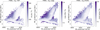 |
Fig. 6 Kiel diagram for the final catalog, colored with the estimated errors on the three parameters. From left to right: Teff, log ɡ, and [Fe/H]. The diagram is divided into small hexagonal bins, and the color represents the average of the error inside the bin. |
Second release of the Survey of Surveys, containing the SoS-Spectro and the SoS-ML catalogs.
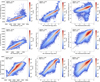 |
Fig. 7 Comparison of the atmospheric parameters predicted by our ML approach (abscissae) and literature ML catalogs (ordinates). The left plots show Teff comparisons, the middle plots show log g, and the right plots show [Fe/H], The top row shows the comparison with Zhang et al. (2023). the middle row shows the comparison with Gu et al. (2025), and the bottom row shows the comparison with Andrae et al. (2023). The dashed line represents the 1:1 relation. |
6 Science validation
We carried out several tests to validate our results, to understand the strengths and weaknesses of our catalog, and to compare with other literature sources. We discuss the comparisons with other ML methods and the validation with star clusters below. Other validation tests are presented in Appendix C.
6.1 Comparison with Zhang et al
Zhang et al. (2023) employed machine-learning to obtain atmospheric parameters from Gaia XP spectra. They used a data-driven forward model trained on LAMOST and incorporated near-infrared photometry to reduce degeneracies in the parameter estimation. The approach is based on modeling the Gaia XP spectra with known astrophysical parameters and then inferring the parameters for all Gaia XP spectra.
In the top row of Fig. 7, we compare the parameters obtained in this work with those by Zhang et al. (2023). We focus on the stars for which they reported a confidence level higher than 0.5. For the vast majority of stars, we find excellent agreement, with very small trends and biases. There are long tails of discrepant determinations in all three parameters, however, which concern a small fraction of the stars in common. For log ɡ, some objects in Zhang et al. (2023) display values that extend up to 8, which is significantly higher than the typical range for main-sequence stars and giants. Similarly, we observe discrepancies in [Fe/H] values, which reach values as low as −7 dex in Zhang et al. (2023). Metallicities lower than −4 are not typical for the majority of stars and would be considered extreme. They would correspond to rare, very old stars or, most likely, artifacts in the data, as the LAMOST survey does not have metallicity values lower than −2.5. Stars exhibiting extreme log ɡ and [Fe/H] values are the same objects, supporting the idea that these may be artifacts in the Zhang et al. (2023) results. This cannot be said with confidence about the major offset in effective temperatures, however. Most stars in the hot-star subset identified in their work agree well with our results for other parameters. It is worth noting here that the subset of hot stars identified by Zhang et al. (2023) is concentrated near the Galactic plane. Since effective temperature estimates depend on accurate extinction corrections, it is difficult to determine which set of Teff values is more reliable in this case.
6.2 Comparison with Gu et al
The second release of the SAGES database (Gu et al. 2025) presents an ML derivation of stellar parameters for over 21 million stars based on a vast compilation of data obtained by integrating spectroscopic estimates and high-resolution data from the literature with photometric observations from SAGES DR1 (Fan et al. 2023), Gaia DR3 (Gaia Collaboration 2023), All-WISE (Cutri et al. 2021), 2MASS (Cutri et al. 2003), and GALEX (Bianchi et al. 2014). They employed an ML approach based on the random forest algorithm to infer Teff, log ɡ, and metallicity. As labels, the data from LAMOST DR10 (Zhao et al. 2012) and APOGEE DR17 (Abdurro'uf et al. 2022) were used, augmented with the data from PASTEL (Soubiran et al. 2016) and RAVE DR5 (Kunder et al. 2017).
Because the method and size of the resulting catalog is similar with ours, the comparison with the SAGE catalog is particularly relevant; it is shown in the middle row of Fig. 7 and agrees very well. There are no significant groups of outliers, unlike in the comparison with Zhang et al. (2023). We only noted a small trend in Teff that is qualitatively similar to the trend in the comparison with Zhang et al. (2023), but completely different from the trend in the comparison with Andrae et al. (2023). The observed trend appears to be well within the combined uncertainties reported in the catalogs (<150 K at the extremes), but it would be interesting to explore this feature further in the future.
6.3 Comparison with Andrae et al
In our ML approach, we used the metallicity [Fe/H] from Andrae et al. (2023) as an input parameter because their metallicities agree better with the SoS-Spectro and PASTEL than the Gaia DR3 GSP-Phot metallicities. We did not use their Teff and log ɡ values, and a comparison is therefore still relevant. Andrae et al. (2023) applied the XGBoost machine-learning algorithm to publicly available Gaia XP spectra and trained their model on stellar parameters from the APOGEE survey, complemented with a set of very metal-poor stars. Their catalog is far larger than ours and comprises 175 million stars.
The bottom row of Fig. 7 shows the comparison. While the [Fe/H] values agree extremely well, as expected, because we used them as input parameters to the ML prediction, we observe a large spread. Combined with our favorable comparison with star clusters (Sect. 6.4), this shows that by building upon the work by Andrae et al. (2023), we were indeed able to obtain improved predictions with our approach. On the other hand, we observe striking patterns in the comparison with Teff and log ɡ that are absent in the comparisons with Zhang et al. (2023) and Gu et al. (2025). Interestingly, Gu et al. (2025) observe the same patterns in the comparison of their log g values with those from Andrae et al. (2023), which indicates features in the Andrae et al. (2023) catalog rather than in ours.
6.4 Validation on star clusters
To further test our metallicity predictions, we validated our results using a sample of globular and open clusters. For globular clusters, the metallicities we used for the validation were taken from Harris (1996), while we selected probable members using Vasiliev & Baumgardt (2021) with a membership probability threshold of 0.8. We focused on 20 globular clusters with more than 20 members with ML predictions in our catalog. For open clusters, we used high-quality metallicities from Netopil et al. (2016), and we selected members based on Hunt & Reffert (2024). As with the globular clusters, we focused on 16 open clusters with more than 20 members in our ML sample. In Fig. 8, we extended the comparison to the other ML catalogs examined in the previous sections using the same clusters, reference metallicities, and member selection procedure.
For globular clusters, which are notoriously difficult to parameterize correctly with ML methods or even in the typical spectroscopic surveys, our predictions are excellent, and they appear to have smaller offsets from Harris (1996) and smaller spreads compared to those of the other ML methods. Additionally, our predictions are equally good at all metallicities, unlike in the case of other ML methods. This proves that our approach of building upon previous work (in this case by Andrae et al. 2023) to improve on it instead of starting from scratch is suitable to improve the predictions at the low-metallicity end. Our recalibration of the SoS-Spectro on PASTEL probably also played an important role by improving the [Fe/H] reference values for metal-poor giants, and thus, for globular clusters.
For open clusters, we observe an underestimation in the predictions of all ML methods, except for Gu et al. (2025). The offset is about −0.1 dex or slightly more, depending on the method. Despite their better mean values, the spread in the predictions by Gu et al. (2025) within each cluster is larger. A detailed cluster-by-cluster and star-by-star comparison is presented in Appendix D. Our approach appears to perform similarly well to the other methods at solar metallicity, with a small improvement on the spread within each cluster compared to other ML methods, and with a small improvement on the zeropoint compared to our input dataset from Andrae et al. (2023). Concerning the observed offset with Netopil et al. (2016), the extremely similar behavior among the different ML methods suggests that the observed systematics might stem from the catalog by Netopil et al. (2016). We thus tried to compare our results to other literature sources, such as Dias et al. (2021) or Kharchenko et al. (2013), which is a compilation of metallicities from other sources, but we obtained very similar −0.1 dex offsets. The origin of the offsets therefore currently remains unexplained.
7 Conclusions
We presented the second release of the SoS catalog. It contains atmospheric parameters, namely Teff, log ɡ, and [Fe/H], for about 23 million stars, with estimated formal errors of about 50 K for Teff and about 0.07–0.08 dex for log ɡ and [Fe/H]. The catalog is composed of two parts: SoS-Spectro and SoS-ML. The SoS-Spectro catalog (Sect. 3) is the result of a simple homogenization procedure applied to the same five spectroscopic surveys as in Tsantaki et al. (2022), recalibrated on the high-resolution spectroscopy analysis collected by Soubiran et al. (2016) in PASTEL.
The SoS-ML catalog (Sect. 5) is the result of a ML method application to enhance previous estimates of stellar parameters, that is, to improve their precision and accuracy. In particular, we relied on Teff and log ɡ estimates by Gaia DR3 and [Fe/H] estimates by Andrae et al. (2023). We used large photometry surveys, such as SDSS and SM, to refine the parameters. This was also made possible by leveraging the large Gaia DR3 dataset with precise astrometry and photometry, which was also key to our accurate cross-match between catalogs. We selected a very simple multilayer perceptron architecture (Sect. 4) that yielded extremely good results, even compared with the recent literature (Sect. 6). Compared to previous efforts in deriving stellar parameters with ML, our method has two main differences. The first key ingredient is the SoS-Spectro reference catalog, which is recalibrated on high-resolution spectroscopy: Our model was trained on the SoS values to accurately reproduce them from the photometric inputs. The second ingredient is that we did not try to predict the parameters from scratch, but built on previous estimates by Gaia DR3 and Andrae et al. (2023).
To summarize our validation results (Sect. 6 and Appendix C), our results compare extremely well with other ML catalogs in the literature for the vast majority of stars in common. We lack some of the samples of spurious determinations that are visible in other catalogs, however. Additionally, our results show a smaller spread, that is, our internal errors (precision) are smaller. Our catalog size is comparable with the sizes of some ML catalogs in the literature (e.g., Zhang et al. 2023; Gu et al. 2025), but is smaller by one order of magnitude than Andrae et al. (2023) and smaller by two orders of magnitude than Gaia DR3. For star clusters, we perform similarly well as or slightly better than other ML methods at solar metallicity, but the improvement in the globular cluster metallicity range in accuracy and precision is striking. We also tried to improve on the problems of ML methods at even lower metallicities by augmenting our training set with a few hundred very metal-poor stars ([Fe/H] ≲ −2 dex; Appendix C.1), but this only produced a slight improvement at all metallicities and failed to solve the problem.
In future work, we will try to address the problems at very low metallicities, but also work to increase the sample sizes by including more photometric and spectroscopic surveys. An addition of abundance ratios to the list of parameters would surely be a worthwhile goal. It is also vital in general to refine the extinction and distance inputs to improve on the quality and quantity of the predictions. Finally, several additional improvements can be achieved by using more sophisticated algorithmic approaches that make use of precategorization, clustering, and feature enhancement.
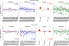 |
Fig. 8 Comparison of metallicity predictions for globular (top row) and open clusters (bottom row). Our results are shown in purple in the leftmost panels, the results by Andrae et al. (2023) are plotted in blue in the center left panels, the results by Gu et al. (2025) are shown in red in the center right panels, and the results by Zhang et al. (2023) are shown in green in the rightmost panels. The boxplots show the metallicity differences with respect to the values reported by Harris (1996) and Netopil et al. (2016) for selected clusters. The boxes represent the interquartile range (IQR), the central lines the median, and the whiskers extend to 1.5 times the IQR. Outliers are marked as individual points. The mean metallicity difference (M) and standard deviation (Σ) are annotated in each panel. The dashed line at zero indicates perfect agreement with the literature values (zero-line). Clusters are sorted by ascending metallicity. |
Data availability
The SoS DR2 catalog is available at the CDS via https://cdsarc.cds.unistra.fr/viz-bin/cat/J/A+A/700/A195 and on the SoS portal at the Space Science Data Center https://gaiaportal.ssdc.asi.it/SoS2.
Acknowledgements
People. We acknowledge interesting exchanges of ideas with our colleagues: G. Battaglia, S. Fabbro, I. Gonzalez Rivera, G. Kordopatis, M. Valentini. Funding. Funded by the European Union (ERC-2022-AdG, “Star-Dance: the non-canonical evolution of stars in clusters”, Grant Agreement 101093572, PI: E. Pancino). Views and opinions expressed are however those of the author(s) only and do not necessarily reflect those of the European Union or the European Research Council. Neither the European Union nor the granting authority can be held responsible for them. We also acknowledge the financial support to this research by INAF, through the Mainstream Grant “Chemo-dynamics of globular clusters: the Gaia revolution” (no. 1.05.01.86.22, P.I. E. Pancino). We are thankful for the team meetings at the International Space Science Institute (Bern) for fruitful discussions and were supported by the ISSI International Team project “AsteroSHOP: large Spectroscopic surveys HOmogenisation Program” (PI: G. Thomas). EP acknowledges financial support from PRIN-MIUR-22: CHRONOS: adjusting the clock(s) to unveil the CHRONO-chemo-dynamical Structure of the Galaxy” (PI: S. Cassisi) funded by the European Union – Next Generation EU. MT thanks INAF for the Large Grant EPOCH and the Mini-Grant PILOT (1.05.23.04.02). PMM and SM acknowledge financial support from the ASI-INAF agreement no. 2022-14-HH.0. GFT acknowledges support from the Agencia Estatal de Investigación del Ministerio de Ciencia en Innovación (AEI-MICIN) and the European Regional Development Fund (ERDF) under grant numbers PID2020-118778GB-I00/10.13039/501100011033 and PID2023-150319NB-C21/C22 and the AEI under grant number CEX2019-000920-S. GG acknowledges support by Deutsche Forschungs-gemeinschaft (DFG, German Research Foundation) – project-IDs: eBer-22-59652 (GU 2240/1-1 “Galactic Archaeology with Convolutional Neural-Networks: Realising the potential of Gaia and 4MOST”). This project has received funding from the European Research Council (ERC) under the European Union’s Horizon 2020 research and innovation programme (Grant agreement No. 949173). FG gratefully acknowledges support from the French National Research Agency (ANR) funded projects “MWDisc” (ANR-20-CE31-0004) and “Pristine” (ANR-18-CE31-0017) Data. This work has made use of data from the European Space Agency (ESA) mission Gaia (https://www.cosmos.esa.int/gaia), processed by the Gaia Data Processing and Analysis Consortium (DPAC, https://www.cosmos.esa.int/web/gaia/dpac/consortium). Funding for the DPAC has been provided by national institutions, in particular the institutions participating in the Gaia Multilateral Agreement. Funding for the Sloan Digital Sky Survey IV has been provided by the Alfred P. Sloan Foundation, the U.S. Department of Energy Office of Science, and the Participating Institutions. SDSS-IV acknowledges support and resources from the Center for High Performance Computing at the University of Utah. The national facility capability for SkyMapper has been funded through ARC LIEF grant LE130100104 from the Australian Research Council, awarded to the University of Sydney, the Australian National University, Swinburne University of Technology, the University of Queensland, the University of Western Australia, the University of Melbourne, Curtin University of Technology, Monash University and the Australian Astronomical Observatory. Software. Most of the plotting and data analysis was carried out using R (R Core Team 2017; Dowle & Srinivasan 2017) and Python (Chollet et al. 2015; Abadi et al. 2015).This research has made use of the SIMBAD database (Wenger et al. 2000) and the VizieR catalogue access tool (Ochsenbein et al. 2000), both operated at CDS, Strasbourg, France. Preliminary data exploration relied heavily on TopCat (Taylor 2005).
Appendix A Systematics among survey releases
In this section, we present a detailed comparison of the SoS-Spectro parameters with the most recent updates from the APOGEE DR17, GALAH DR4, and LAMOST DR10 surveys. As previously mentioned, the SoS-Spectro parameters are based on earlier data releases, which can lead to systematic biases when compared with the most recent versions. To ensure a fair comparison with high-quality data, we apply the following selection criteria, as recommended by the survey authors:
APOGEE DR17: aspcapflag ≠ star_bad
GALAH DR4: flag_sp = 0, flag_fe_h = 0, snr_px_ccd3 > 30
LAMOST DR10: snr > 30
Figure A.1 illustrates the differences between the SoS-Spectro parameters and the latest survey releases. The plots also include comparisons between the original data releases used in SoS-Spectro and the latest versions of each survey. We found that the systematic differences appear as wavy-like patterns when plotted against the absolute G-band magnitude from Gaia DR3. The typical differences between SoS-Spectro parameters and those from APOGEE DR17, GALAH DR4, and LAMOST DR10 are summarized in Table A.1. These observed differences reflect substantial improvements in the latest APOGEE and GALAH datasets. APOGEE DR17 features a reworked ASPCAP pipeline, a new synthetic spectral grid including NLTE effects, and auxiliary analyses using alternative libraries. GALAH DR4 benefits from a more stable wavelength calibration (especially near CCD edges) and enhanced outlier detection, yielding more reliable spectroscopic parameters.
More in details, in the comparison with GALAH DR4, the data show increased variability, with wider interquartile range (IQR) compared to APOGEE, especially in Teff and logɡ. Notably, greater scatter in logɡ is observed among stars brighter than MG = 0. Despite this variability, the median offsets remain small, indicating overall consistency between SoS-Spectro and GALAH parameters.
Finally, we compared SoS-Spectro parameters with LAM-OST DR10. While logɡ shows negligible median deviation, a systematic offset of 0.05 dex is found between [Fe/H] values in DR5 and DR10, indicating a shift in calibration. The offset in Teff between SoS-Spectro and DR10 is also clear and cannot be solely explained by differences with DR5. This offset originates from the specific corrections applied to LAMOST DR5 temperatures during the construction of the SoS-Spectro catalog.
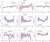 |
Fig. A.1 Differences in Teff, log g, and [Fe/H] between earlier and later data releases of three major spectroscopic surveys. Top: APOGEE DR16 vs DR17 (orange) and SoS-Spectro vs DR17 (blue); middle: GALAH DR2 vs DR4 (magenta) and SoS-Spectro vs DR4 (blue); bottom: LAMOST DR5 vs DR10 (pink) and SoS-Spectro vs DR10 (blue). Square markers denote internal survey updates, round markers show differences with SoS-Spectro, and shaded regions represent the interquartile range of residuals. These comparisons reveal that the SoS-Spectro discrepancies are of similar or smaller scale than the internal changes across survey versions. |
Appendix B Uncertainties in SDSS and SM
The training and application datasets are composed of two distinct parts based on SDSS and SM photometry. While the main text presents the combined results for clarity, this appendix provides the separate results for each survey, offering a more detailed view of the model performance.
In figure B.1, we show the Kiel diagrams obtained on the full SDSS and SM catalogs, as selected in sections 2.2 and 2.3 and colored with the estimated error eML on each parameter Teff, logɡ, and [Fe/H]. The error value is dominated by erep and thus indicate the repeatability of the prediction and the solidity of the model solution for the stars in that region of the parameter space. It is to be expected that the regions which have poor or no coverage within the training sample (indicated by the black line in Fig. B.1) show the largest error.
Comparison of SoS-Spectro parameters with the latest versions of the surveys.
In figure B.2, we show the distributions of eML for the three parameters over each dataset. We notice that the distribution of [Fe/H] errors on the SM dataset has larger tails, which however are several order of magnitudes less populous than the distribution peak and thus do not affect significantly the global median or mean error.
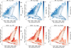 |
Fig. B.1 Kiel Diagram for the SM (above) and SDSS (below) full sample, colored with the estimated errors on the three parameters. From left to right: Teff, log ɡ, and [Fe/H]. Hexagonal bins are colored based on the average of the errors inside the bin. The black line approximately encloses the region covered by the respective “train_area” flags described in Sect. 5.2. |
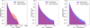 |
Fig. B.2 Distribution of EML SM dataset (green) and the SDSS dataset (red). The y scale indicates the logarithm of the fraction of the dataset in each bin (total of 100 bins). |
Appendix C Additional validation
C.1 Very metal-poor stars
If spectroscopic surveys and ML methods have trouble predicting [Fe/H] for metal-poor stars, in particular giants, this is even more pronounced in the case of very metal-poor stars, i.e., stars with [Fe/H] ≲ −2 dex. Fig. C.1 illustrates the problem for our catalog as well as the ones by Zhang et al. (2023), Andrae et al. (2023), and Gu et al. (2025). The effect is observed both in the comparison with PASTEL and with the SAGA database (Suda et al. 2008). We tried to tackle the problem by augmenting the training sets for SDSS and SM with a few hundred very metal-poor stars selected from PASTEL (Sect. 4.2). The results before (grey) and after (purple) adding the stars are shown in the left panels of Fig. C.1. As can be seen, their addition to the training sample did not solve the problem with the very metal-poor stars, but it did slightly improve our [Fe/H] estimates over the entire metallicity range.
C.2 White dwarfs
Our training sample does not include any white dwarf star (WD), but it is reasonable to expect that some WD might be present in the photometric catalogs and they could in principle have been wrongly parameterized. To verify that there are no WD in our final catalog, we cross-matched it with two published WD catalogs. The first is the Gentile Fusillo et al. (2021) catalog, which contains more than 1.2 million WDs and is based on Gaia DR3. A cross-match with this catalog yielded no common objects, suggesting that our catalog is indeed free from WDs. The second is the recently published single and binary WD catalog by Jackim et al. (2024), which identifies single and binary WDs using GALEX UV color magnitude diagrams. The cross-match identified 40 276 objects in our final catalog, only 200 of which are classified as single WDs by Jackim et al. (2024). However, when these objects are plotted on the HR diagram, they fall outside the WD locus (see Fig. C.2). Instead, they are distributed in regions associated with main-sequence stars or other stellar populations. This suggests that these objects are not single WD, but likely the non-WD components of binary systems, or alternatively stars that display UV excess because they are chromospherically active. Notably, none of these objects exhibit increased errors or abnormal properties, suggesting that their UV excess does not significantly impact their optical properties.
C.3 Gravity comparison with APOKASC
The third APOKASC (APOKASC-3) catalog (Pinsonneault et al. 2025) provides a comprehensive dataset for 15808 evolved stars, combining spectroscopic parameters from APOGEE with asteroseismic measurements from NASA’s Kepler mission (Borucki 2016). Of these, detailed parameters such as stellar evolutionary state, surface gravity, mass, radius, and age are available for 12418 stars, calibrated using Gaia luminosities and APOGEE spectroscopic effective temperatures.
The catalog features precise asteroseismic measurements with median fractional uncertainties of 0.6% in vmax and ∆v, and 1.8% in radius, making it a reliable resource for validating derived stellar parameters. Given its robust calibration and high data quality, APOKASC-3 is well-suited for testing log ɡ values, providing a consistent and independent benchmark for stellar characterization studies.
Fig. C.3 shows the comparison between the surface gravity log ɡ values estimated in APOKASC-3 and those predicted in our work. The error bars on our predictions represent the associated uncertainties. As can be seen, a systematic offset is present, albeit the few stars in common, with a median difference of 0.14 dex and with the errorbars barely touching the 1:1 line. The effect is visible especially for giants with log ɡ ≲ 2.5 dex. This difference is consistent with the offset observed between the SoS-Spectro dataset (used as a reference for ML training) and high-quality log ɡ measurements from the PASTEL catalog (see Fig.3). Such discrepancies likely results from general inconsistencies in the determination of log ɡ for giant stars across large spectroscopic surveys, which are impacted also by NLTE effects, especially at low metallicity. Our recalibration of the SoS-Spectro on PASTEL was not sufficient to erase this trend with log ɡ, unlike what happened for [Fe/H] in the case of globular clusters. This remains one important challenge for the future SoS data releases and for spectroscopic surveys and ML methods in general.
C.4 Validation of cool star temperatures using spectral types
Among the most striking features in the comparisons presented in Sect. 6 is the difference in Teff with Andrae et al. (2023), particularly for the cool stars in our catalog. To explore this discrepancy, we selected stars with ML-predicted Teff < 3400 K and cross-matched them with the Simbad database8. Among these, we identified approximately 700 stars with spectral types ranging from M2 to M6, the majority being classified as M4V. We grouped the spectral types into rounded categories and calculated the median effective temperature for each group using both our ML predictions and the estimates of Andrae et al. (2023).
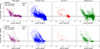 |
Fig. C.1 Comparison of the [Fe/H] predicted by this work and by three literature ML catalogs with the PASTEL (top row) and SAGA (bottom row) databases. Our results are shown in the leftmost plots, where the grey points show the results before, and the purple ones after, augmenting the reference SoS-Spectro catalog with very metal-poor stars. The median [Fe/H] differences for the before and after augmentation samples (computed only for [Fe/H] < −2) are indicated in the top-left corner of the first plot in each row. A similar comparison is presented for the following catalogs: Andrae et al. (2023, blue, center-left panels), Gu et al. (2025, red, center-right panels), and Zhang et al. (2023, green, rightmost panels). |
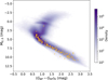 |
Fig. C.2 HR diagram showing the distribution of objects from our final catalog. MG is calculated using parallax. Yellow stars indicate 200 single UV-excess objects from Jackim et al. (2024) found in our catalog. |
Fig. C.4 presents these medians, along with the range of temperature estimates shown as whiskers. For reference, we also include the Teff for each spectral type as provided by Pecaut & Mamajek (2013). It is important to note that these values are strictly valid for main-sequence stars, while our sample may contain a few giants and several pre-main sequence stars. Nonetheless, they offer a reasonable benchmark for Teff estimates based on spectral type. In this regard, our results align more closely with the known spectral classifications.
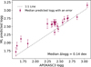 |
Fig. C.3 Comparison of surface gravity log g values by APOKASC-3 with those predicted using machine learning in this study. The error bars represent the uncertainties in our predictions. |
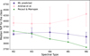 |
Fig. C.4 Calculated median effective temperatures and their range (whiskers) for each spectral type from Andrae et al. (pink squares) and as predicted in this paper (purple diamonds). The values provided by Pecaut & Mamajek are shown as green stars. |
Appendix D Cluster by cluster [Fe/H] comparisons
In this section, we present a cluster-by-cluster comparison of the [Fe/H] estimates derived in this work with those obtained from external ML-based studies. We adopt the same cluster membership selections and literature metallicity values as in Sect. 6.
D.1 Globular clusters
Under these criteria, 20 globular clusters are retained, although only two (NGC 7078 and NGC 7079) have sufficient data from Gu et al. (2025) to be included. Figure D.1 shows, for each group, the distribution of differences between the estimated [Fe/H] values and the metallicities in the Harris (1996) catalog. Each subplot presents histograms of the residuals for each data source, allowing a direct visual comparison across ML methods. The histograms are normalized by the number of objects in each dataset to account for differences in sample size. As can be seen, our method generally produces narrower and more centered residual distributions, indicating improved consistency with reference metallicities.
Nevertheless, some clusters exhibit notable deviations from Harris, which merit further discussion. NGC 288 shows systematically higher metallicities across all data sources, consistent with the results of Mészáros et al. (2020), who report a 0.136 dex offset from Harris. For NGC 7078 (M 15), both the mean and scatter are elevated, which may reflect the large discrepancies found between LTE and NLTE abundance estimates in this cluster (Kovalev et al. 2019). In the case of NGC 6218, Harris (1996) reports [Fe/H] = −1.37, while APOGEE-based studies find systematically higher values (−1.26 to −1.27; Horta et al. 2020; Schiavon et al. 2024), suggesting possible systematic offsets in either APOGEE or the Harris (1996) compilation. It is worth mentioning that our results tend to align more closely with those reported by Schiavon et al. (2024) than with the Harris (1996) catalog. This agreement may stem from the fact that recent catalogue of Schiavon et al. (2024) make use of APOGEE-based measurements, and our estimates are also based on spectroscopic surveys. For NGC 3201, although our mean metallicity agrees with both Harris and Schiavon et al. (2024), the large difference between their reference values (−1.59 and −1.39, respectively) may explain the broader residual distribution we observe. Similarly, NGC 5139 (ω Cen) shows a higher dispersion, although this is expected due to its complex internal metallicity distribution.
A few clusters show sligthly larger spreads in our SoS-ML catalog. NGC 6254 exhibits a larger scatter in our results compared to other surveys. A similar trend was noted by Pagnini et al. (2025), who reported a dispersion of 0.07 dex, slightly lower than what we observe. However, their estimate assumes that the ASPCAP uncertainties are reliable. This assumption may not hold, as previous analyses have shown that APOGEE’s reported uncertainties can be significantly underestimated, with the three-cornered hat method revealing much larger true errors (Tsantaki et al. 2022). NGC 7099 and NGC 6752 both display slightly elevated or broadened residuals across data sources without any clear explanation in the literature.
D.2 Open clusters
Following the criteria described above, we used the members list by Hunt & Reffert (2024) and compared our results with the homogeneous mean cluster metallicities compiled by Netopil et al. (2016), based on high-resolution spectroscopy. We used 16 open clusters with more than 20 bona fide members. As reported in Sect. 6.4, all the ML methods show an average offset with the reference mean [Fe/H] for the selected open clusters. The same offset remained when comparing against different catalogs, such as Kharchenko et al. (2016) or Dias et al. (2021).
The cluster-by-cluster comparisons are shown in Fig. D.2. They generally confirm the agreement among the ML methods, with the only exception of NGC 1817, where the results by Gu et al. (2025) appear to have a smaller bias and a larger spread. We also note a general tendency of our predictions to have a smaller spread and fewer outliers in the distributions of each cluster, similarly to what observed for globular clusters, but in a less pronounced way. This confirms that we could improve slightly on the precision of the predicted [Fe/H] values in the range of Solar metallicity, but not on the bias, compared to other methods.
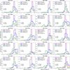 |
Fig. D.1 The [Fe/H] differences between predictions from various ML methods and Harris (1996) reference values for globular clusters. Each panel represents a cluster, with histograms of [Fe/H] differences for the four ML methods explored in Sect. 6: this paper, Andrae et al. (2023), Zhang et al. (2023), and Gu et al. (2025). The mean and standard deviation of the differences are annotated only for our method. |
References
- Abadi, M., Agarwal, A., Barham, P., et al. 2015, TensorFlow: Large-Scale Machine Learning on Heterogeneous Systems, software available from https://tensorflow.org [Google Scholar]
- Abazajian, K., Adelman-McCarthy, J. K., Agüeros, M. A., et al. 2003, AJ, 126, 2081 [Google Scholar]
- Abdurro’uf, Accetta, K., Aerts, C., et al. 2022, ApJS, 259, 35 [NASA ADS] [CrossRef] [Google Scholar]
- Ahumada, R., Allende Prieto, C., Almeida, A., et al. 2020, ApJS, 249, 3 [NASA ADS] [CrossRef] [Google Scholar]
- Albareti, F. D., Allende Prieto, C., Almeida, A., et al. 2017, ApJS, 233, 25 [Google Scholar]
- Anders, F., Khalatyan, A., Guiglion, G., et al. 2022, in EAS2022, European Astronomical Society Annual Meeting, 1891 [Google Scholar]
- Andrae, R., Rix, H.-W., & Chandra, V. 2023, ApJS, 267, 8 [NASA ADS] [CrossRef] [Google Scholar]
- Bailer-Jones, C. A. L., Rybizki, J., Fouesneau, M., Demleitner, M., & Andrae, R. 2021, AJ, 161, 147 [Google Scholar]
- Bianchi, L., Conti, A., & Shiao, B. 2014, Adv. Space Res., 53, 900 [Google Scholar]
- Borucki, W. J. 2016, Rep. Progr. Phys., 79, 036901 [Google Scholar]
- Buder, S., Asplund, M., Duong, L., et al. 2018, MNRAS, 478, 4513 [Google Scholar]
- Chollet, F., et al. 2015, Keras, https://keras.io [Google Scholar]
- Cutri, R. M., Skrutskie, M. F., van Dyk, S., et al. 2003, VizieR Online Data Catalog: 2MASS All-Sky Catalog of Point Sources (Cutri+ 2003), VizieR On-line Data Catalog: II/246. Originally published in: University of Massachusetts and Infrared Processing and Analysis Center, (IPAC/California Institute of Technology) [Google Scholar]
- Cutri, R. M., Wright, E. L., Conrow, T., et al. 2021, VizieR Online Data Catalog: AllWISE Data Release (Cutri+ 2013), VizieR On-line Data Catalog: II/328. Originally published in: IPAC/Caltech [Google Scholar]
- Deng, L.-C., Newberg, H. J., Liu, C., et al. 2012, Res. Astron. Astrophys., 12, 735 [Google Scholar]
- Dias, W. S., Monteiro, H., Moitinho, A., et al. 2021, MNRAS, 504, 356 [NASA ADS] [CrossRef] [Google Scholar]
- Dowle, M., & Srinivasan, A. 2017, data.table: Extension of ‘data.frame’, https://CRAN.R-project.org/package=data.table [Google Scholar]
- Fabbro, S., Venn, K. A., O’Briain, T., et al. 2018, MNRAS, 475, 2978 [Google Scholar]
- Fan, Z., Zhao, G., Wang, W., et al. 2023, ApJS, 268, 9 [NASA ADS] [CrossRef] [Google Scholar]
- Gaia Collaboration (Vallenari, A., et al.) 2023, A&A, 674, A1 [NASA ADS] [CrossRef] [EDP Sciences] [Google Scholar]
- Gentile Fusillo, N. P., Tremblay, P. E., Cukanovaite, E., et al. 2021, MNRAS, 508, 3877 [NASA ADS] [CrossRef] [Google Scholar]
- Gilmore, G., Randich, S., Asplund, M., et al. 2012, The Messenger, 147, 25 [NASA ADS] [Google Scholar]
- Gu, H., Fan, Z., Zhao, G., et al. 2025, ApJS, 277, 19 [Google Scholar]
- Guiglion, G., Nepal, S., Chiappini, C., et al. 2024, A&A, 682, A9 [NASA ADS] [CrossRef] [EDP Sciences] [Google Scholar]
- Harris, W. E. 1996, AJ, 112, 1487 [Google Scholar]
- Horta, D., Schiavon, R. P., Mackereth, J. T., et al. 2020, MNRAS, 493, 3363 [NASA ADS] [CrossRef] [Google Scholar]
- Huang, Y., Yuan, H., Li, C., et al. 2021, ApJ, 907, 68 [NASA ADS] [CrossRef] [Google Scholar]
- Hunt, E. L., & Reffert, S. 2024, A&A, 686, A42 [NASA ADS] [CrossRef] [EDP Sciences] [Google Scholar]
- Jackim, R., Heyl, J., & Richer, H. 2024, arXiv e-prints [arXiv:2404.07388] [Google Scholar]
- Keller, S. C., Schmidt, B. P., Bessell, M. S., et al. 2007, PASA, 24, 1 [NASA ADS] [CrossRef] [Google Scholar]
- Kharchenko, N. V., Piskunov, A. E., Schilbach, E., Röser, S., & Scholz, R. D. 2013, A&A, 558, A53 [NASA ADS] [CrossRef] [EDP Sciences] [Google Scholar]
- Kharchenko, N. V., Piskunov, A. E., Schilbach, E., Röser, S., & Scholz, R. D. 2016, A&A, 585, A101 [NASA ADS] [CrossRef] [EDP Sciences] [Google Scholar]
- Kovalev, M., Bergemann, M., Ting, Y.-S., & Rix, H.-W. 2019, A&A, 628, A54 [NASA ADS] [CrossRef] [EDP Sciences] [Google Scholar]
- Kunder, A., Kordopatis, G., Steinmetz, M., et al. 2017, AJ, 153, 75 [Google Scholar]
- Lindegren, L., Klioner, S. A., Hernandez, J., et al. 2021, A&A, 649, A2 [NASA ADS] [CrossRef] [EDP Sciences] [Google Scholar]
- Mannucci, F., Pancino, E., Belfiore, F., et al. 2022, Nat. Astron., 6, 1185 [NASA ADS] [CrossRef] [Google Scholar]
- Marrese, P. M., Marinoni, S., Fabrizio, M., & Giuffrida, G. 2017, A&A, 607, A105 [NASA ADS] [CrossRef] [EDP Sciences] [Google Scholar]
- Marrese, P. M., Marinoni, S., Fabrizio, M., & Altavilla, G. 2019, A&A, 621, A144 [NASA ADS] [CrossRef] [EDP Sciences] [Google Scholar]
- Mészáros, S., Masseron, T., García-Hernández, D. A., et al. 2020, MNRAS, 492, 1641 [Google Scholar]
- Ness, M., Hogg, D. W., Rix, H. W., Ho, A. Y. Q., & Zasowski, G. 2015, ApJ, 808, 16 [NASA ADS] [CrossRef] [Google Scholar]
- Netopil, M., Paunzen, E., Heiter, U., & Soubiran, C. 2016, A&A, 585, A150 [NASA ADS] [CrossRef] [EDP Sciences] [Google Scholar]
- Ochsenbein, F., Bauer, P., & Marcout, J. 2000, A&AS, 143, 23 [NASA ADS] [CrossRef] [EDP Sciences] [Google Scholar]
- Pagnini, G., Di Matteo, P., Haywood, M., et al. 2025, A&A, 693, A155 [NASA ADS] [CrossRef] [EDP Sciences] [Google Scholar]
- Pancino, E., Marrese, P. M., Marinoni, S., et al. 2022, A&A, 664, A109 [NASA ADS] [CrossRef] [EDP Sciences] [Google Scholar]
- Pecaut, M. J., & Mamajek, E. E. 2013, ApJS, 208, 9 [Google Scholar]
- Pinsonneault, M. H., Zinn, J. C., Tayar, J., et al. 2025, ApJS, 276, 69 [NASA ADS] [CrossRef] [Google Scholar]
- R Core Team 2017, R: A Language and Environment for Statistical Computing, R Foundation for Statistical Computing, Vienna, Austria [Google Scholar]
- Rodrigo, C., Cruz, P., Aguilar, J. F., et al. 2024, A&A, 689, A93 [NASA ADS] [CrossRef] [EDP Sciences] [Google Scholar]
- Scaldelai, D., Matioli, L. C., & and, S. R. S. 2024, J. Appl. Statist., 51, 740 [Google Scholar]
- Schiavon, R. P., Phillips, S. G., Myers, N., et al. 2024, MNRAS, 528, 1393 [CrossRef] [Google Scholar]
- Schlegel, D. J., Finkbeiner, D. P., & Davis, M. 1998, ApJ, 500, 525 [Google Scholar]
- Skrutskie, M. F., Cutri, R. M., Stiening, R., et al. 2006, AJ, 131, 1163 [NASA ADS] [CrossRef] [Google Scholar]
- Soubiran, C., Le Campion, J.-F., Brouillet, N., & Chemin, L. 2016, A&A, 591, A118 [NASA ADS] [CrossRef] [EDP Sciences] [Google Scholar]
- Soubiran, C., Brouillet, N., & Casamiquela, L. 2022, A&A, 663, A4 [NASA ADS] [CrossRef] [EDP Sciences] [Google Scholar]
- Steinmetz, M., Zwitter, T., Siebert, A., et al. 2006, AJ, 132, 1645 [Google Scholar]
- Steinmetz, M., Guiglion, G., McMillan, P. J., et al. 2020a, AJ, 160, 83 [NASA ADS] [CrossRef] [Google Scholar]
- Steinmetz, M., Matijevic, G., Enke, H., et al. 2020b, AJ, 160, 82 [NASA ADS] [CrossRef] [Google Scholar]
- Suda, T., Katsuta, Y., Yamada, S., et al. 2008, PASJ, 60, 1159 [NASA ADS] [Google Scholar]
- Taylor, M. B. 2005, in Astronomical Society of the Pacific Conference Series, 347, Astronomical Data Analysis Software and Systems XIV, eds. P. Shopbell, M. Britton, & R. Ebert, 29 [NASA ADS] [Google Scholar]
- Ting, Y.-S., Conroy, C., Rix, H.-W., & Cargile, P. 2019, ApJ, 879, 69 [Google Scholar]
- Tsantaki, M., Pancino, E., Marrese, P., et al. 2022, A&A, 659, A95 [NASA ADS] [CrossRef] [EDP Sciences] [Google Scholar]
- Vasiliev, E., & Baumgardt, H. 2021, MNRAS, 505, 5978 [NASA ADS] [CrossRef] [Google Scholar]
- Wenger, M., Ochsenbein, F., Egret, D., et al. 2000, A&AS, 143, 9 [NASA ADS] [CrossRef] [EDP Sciences] [Google Scholar]
- Yanny, B., Rockosi, C., Newberg, H. J., et al. 2009, AJ, 137, 4377 [Google Scholar]
- Zhang, X., Green, G. M., & Rix, H.-W. 2023, MNRAS, 524, 1855 [NASA ADS] [CrossRef] [Google Scholar]
- Zhao, G., Zhao, Y.-H., Chu, Y.-Q., Jing, Y.-P., & Deng, L.-C. 2012, Res. Astron. Astrophys., 12, 723 [NASA ADS] [CrossRef] [Google Scholar]
Defined as MAD = k median(|e − median(e)|), where e is the vector of all the absolute values of the errors e = abs(xpred − xtrue), and k is a scaling factor which is added to rescale the MAD to the standard deviation (i.e., k ≃ 1.4826) for normally distributed data.
The advantage of this choice is that the whole training procedure was run on a simple desktop PC with consumer hardware. After our optimization, each training run took only a few hours of CPU time.
All Tables
Errors of the ML-predicted variables on the test sample with respect to errors from SoS-Spectro.
Second release of the Survey of Surveys, containing the SoS-Spectro and the SoS-ML catalogs.
All Figures
|
Fig. 1 Photometric passbands of Gaia (top panel), SDSS (middle panel), and SkyMapper (bottom panel) as obtained from the SVO filter profile service (Rodrigo et al. 2024, http://svo2.cab.inta-csic.es/theory/fps/). |
| In the text | |
|
Fig. 2 Sky distribution of our sample selections after the cross-match with Gaia and all quality selections (Sect. 2) in an Aitoff projection of RA and Dec. The color scale refers to the density of points (blue is the minimum density, and red is the maximum density). |
| In the text | |
|
Fig. 3 Comparison of the SoS-Spectro atmospheric parameters (Tsantaki et al. 2022, after calibration) with the literature compilation of high-resolution studies in the PASTEL database (Soubiran et al. 2016), for ≃15 000 measurements, corresponding to ≃14 000 unique stars in common (see Sect. 3 for details). The lighter color corresponds to a higher data density per pixel. The gray points in the background represent the uncorrected data before we applied Eq. (2). |
| In the text | |
|
Fig. 4 Distribution of the ML prediction errors on the test dataset in the SM (blue) and SDSS sample case (red). The y-scale indicates the logarithm of the fraction of the training dataset in each bin (a total of 100 bins). |
| In the text | |
|
Fig. 5 Comparison between the ML predictions obtained on the intersection between SDSS and SM training plus test sample and SM sample (55 696 stars). The lighter color corresponds to a higher data density per pixel. |
| In the text | |
|
Fig. 6 Kiel diagram for the final catalog, colored with the estimated errors on the three parameters. From left to right: Teff, log ɡ, and [Fe/H]. The diagram is divided into small hexagonal bins, and the color represents the average of the error inside the bin. |
| In the text | |
|
Fig. 7 Comparison of the atmospheric parameters predicted by our ML approach (abscissae) and literature ML catalogs (ordinates). The left plots show Teff comparisons, the middle plots show log g, and the right plots show [Fe/H], The top row shows the comparison with Zhang et al. (2023). the middle row shows the comparison with Gu et al. (2025), and the bottom row shows the comparison with Andrae et al. (2023). The dashed line represents the 1:1 relation. |
| In the text | |
|
Fig. 8 Comparison of metallicity predictions for globular (top row) and open clusters (bottom row). Our results are shown in purple in the leftmost panels, the results by Andrae et al. (2023) are plotted in blue in the center left panels, the results by Gu et al. (2025) are shown in red in the center right panels, and the results by Zhang et al. (2023) are shown in green in the rightmost panels. The boxplots show the metallicity differences with respect to the values reported by Harris (1996) and Netopil et al. (2016) for selected clusters. The boxes represent the interquartile range (IQR), the central lines the median, and the whiskers extend to 1.5 times the IQR. Outliers are marked as individual points. The mean metallicity difference (M) and standard deviation (Σ) are annotated in each panel. The dashed line at zero indicates perfect agreement with the literature values (zero-line). Clusters are sorted by ascending metallicity. |
| In the text | |
|
Fig. A.1 Differences in Teff, log g, and [Fe/H] between earlier and later data releases of three major spectroscopic surveys. Top: APOGEE DR16 vs DR17 (orange) and SoS-Spectro vs DR17 (blue); middle: GALAH DR2 vs DR4 (magenta) and SoS-Spectro vs DR4 (blue); bottom: LAMOST DR5 vs DR10 (pink) and SoS-Spectro vs DR10 (blue). Square markers denote internal survey updates, round markers show differences with SoS-Spectro, and shaded regions represent the interquartile range of residuals. These comparisons reveal that the SoS-Spectro discrepancies are of similar or smaller scale than the internal changes across survey versions. |
| In the text | |
|
Fig. B.1 Kiel Diagram for the SM (above) and SDSS (below) full sample, colored with the estimated errors on the three parameters. From left to right: Teff, log ɡ, and [Fe/H]. Hexagonal bins are colored based on the average of the errors inside the bin. The black line approximately encloses the region covered by the respective “train_area” flags described in Sect. 5.2. |
| In the text | |
|
Fig. B.2 Distribution of EML SM dataset (green) and the SDSS dataset (red). The y scale indicates the logarithm of the fraction of the dataset in each bin (total of 100 bins). |
| In the text | |
|
Fig. C.1 Comparison of the [Fe/H] predicted by this work and by three literature ML catalogs with the PASTEL (top row) and SAGA (bottom row) databases. Our results are shown in the leftmost plots, where the grey points show the results before, and the purple ones after, augmenting the reference SoS-Spectro catalog with very metal-poor stars. The median [Fe/H] differences for the before and after augmentation samples (computed only for [Fe/H] < −2) are indicated in the top-left corner of the first plot in each row. A similar comparison is presented for the following catalogs: Andrae et al. (2023, blue, center-left panels), Gu et al. (2025, red, center-right panels), and Zhang et al. (2023, green, rightmost panels). |
| In the text | |
|
Fig. C.2 HR diagram showing the distribution of objects from our final catalog. MG is calculated using parallax. Yellow stars indicate 200 single UV-excess objects from Jackim et al. (2024) found in our catalog. |
| In the text | |
|
Fig. C.3 Comparison of surface gravity log g values by APOKASC-3 with those predicted using machine learning in this study. The error bars represent the uncertainties in our predictions. |
| In the text | |
|
Fig. C.4 Calculated median effective temperatures and their range (whiskers) for each spectral type from Andrae et al. (pink squares) and as predicted in this paper (purple diamonds). The values provided by Pecaut & Mamajek are shown as green stars. |
| In the text | |
|
Fig. D.1 The [Fe/H] differences between predictions from various ML methods and Harris (1996) reference values for globular clusters. Each panel represents a cluster, with histograms of [Fe/H] differences for the four ML methods explored in Sect. 6: this paper, Andrae et al. (2023), Zhang et al. (2023), and Gu et al. (2025). The mean and standard deviation of the differences are annotated only for our method. |
| In the text | |
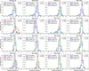 |
Fig. D.2 The same as in Fig. D.1, but for open clusters. |
| In the text | |
Current usage metrics show cumulative count of Article Views (full-text article views including HTML views, PDF and ePub downloads, according to the available data) and Abstracts Views on Vision4Press platform.
Data correspond to usage on the plateform after 2015. The current usage metrics is available 48-96 hours after online publication and is updated daily on week days.
Initial download of the metrics may take a while.