| Issue |
A&A
Volume 701, September 2025
|
|
|---|---|---|
| Article Number | A259 | |
| Number of page(s) | 20 | |
| Section | Planets, planetary systems, and small bodies | |
| DOI | https://doi.org/10.1051/0004-6361/202453124 | |
| Published online | 23 September 2025 | |
Effect of multi-dust species on the inner rim of magnetized protoplanetary disks
1
Max-Planck Institute for Astronomy (MPIA),
Königstuhl 17,
69117
Heidelberg,
Germany
2
Charles University, Fac Math & Phys, Astronomical Institute,
V Holešovičkách 747/2,
180 00
Prague 8,
Czech Republic
3
Center for Astrophysics, Harvard & Smithsonian,
60 Garden Street, M208,
Cambridge,
MA
02138,
USA
4
HUN-REN Research Centre for Astronomy and Earth Sciences, Konkoly Observatory,
Konkoly-Thege Miklós út 15–17,
1121
Budapest,
Hungary
5
CSFK, MTA Centre of Excellence,
Konkoly-Thege Miklós út 15–17,
1121
Budapest,
Hungary
★ Corresponding author: This email address is being protected from spambots. You need JavaScript enabled to view it.
Received:
22
November
2024
Accepted:
31
July
2025
Abstract
Context. Terrestrial planets are born in the inner regions of protoplanetary disks, that is, in the region within ten astronomical units (au). It is crucial to develop multi-physics models of this environment to understand how planets form. By developing a new class of multi-dust radiative magnetized inner rim models and comparing them with recent near-IR observational data, we can gain valuable insights into the conditions during planet formation.
Aims. Our goal is to study the influence of highly refractory dust species on the shape of the inner rim and to determine how the magnetic field affects the structure of the inner disk. The resulting temperature and density structures were analyzed and compared to observations. The comparison focused on the median spectral energy distribution of Herbig stars and interferometric constraints from the H, K, and N bands of three Herbig-type star-disk systems: HD 100546, HD 163296, and HD 169142.
Methods. With the new models, we investigated the influence of a large-scale magnetic field on the structure of the inner disk, and we studied the effect that the four most important dust species (corundum, iron, forsterite, and enstatite) shape the rim, each with its sublimation temperatures. Further, we improved our model by using frequency-dependent irradiation and the effect of accretion heating. With the Optool package, we obtained frequency-dependent opacities for each dust-grain family and calculated the corresponding temperature-dependent Planck and Rosseland opacities.
Results. When multiple dust species are considered, the dust sublimation front, that is, the inner rim, becomes smoother and radially more extended. The emission flux of strongly magnetized disks increases substantially between the L and N bands. Our results show that weakly magnetized disk models with large-scale vertical magnetic fields ≤0.3 Gauss at 1 au best fit with near-IR interferometric observations. Our model comparison supports the existence of moderate magnetic fields (β ≥ 104) that might drive a magnetic wind in the inner disk. Our results show that multi-dust models, including magnetic fields, still lack near-IR emission, especially in the H band. Half-light radii derived from H-band emission by near-IR interferometry indicate that the missing flux originates within the inner rim, where even corundum grains sublimate. One potential solution might be a heated gas disk or evaporating objects such as planetesimals close to the star.
Key words: accretion, accretion disks / hydrodynamics / instabilities / Sun: magnetic fields / planets and satellites: formation / protoplanetary disks
© The Authors 2025
 Open Access article, published by EDP Sciences, under the terms of the Creative Commons Attribution License (https://creativecommons.org/licenses/by/4.0), which permits unrestricted use, distribution, and reproduction in any medium, provided the original work is properly cited.
This article is published in open access under the Subscribe to Open model.
Open Access funding provided by Max Planck Society.
1 Introduction
The formation of planets is one of the most crucial questions of modern astrophysics. More than 5000 exoplanetary systems have been detected so far. The Kepler mission focused on planetary systems around F-, G-, and K-type stars and found that many rocky planets are located close to their host star, at orbital periods of about ten days (Lissauer et al. 2011; Batalha et al. 2013; Fabrycky et al. 2014; Lissauer et al. 2014). Moreover, multi-planet systems show an inner edge, at which the occurrence rate of planets suddenly increases (Mulders et al. 2015; Petigura et al. 2018; Mulders et al. 2018) and which are often composed of super-Earth planets in a compact configuration (Weiss et al. 2023). To understand the formation history of these compact super-Earth planets, we must understand the structure of the inner regions of the protoplanetary disk. In particular, the region in which silicate material sublimates at temperatures of about 1200–1400 K becomes increasingly interesting. Many important astrophysical characteristics come together here. At these locations and radially outward, the disk becomes optically thick to its thermal emission as a result of the condensation of the leading solid material components of iron (Fe), forsterite (Mg2SiO4), and enstatite (MgSiO3) (Woitke et al. 2018). Most of the near-IR continuum flux is emitted at these locations and is seen as a ring structure that is often referenced to the dust rim (Dullemond & Monnier 2010) that is located inside 1 au (Lazareff et al. 2017; GRAVITY Collaboration 2019). Close to this location, the disk is strongly enough ionized for the magne-torotational instability (MRI) to operate (Desch & Turner 2015; Flock et al. 2017; Thi et al. 2019; Lesur et al. 2023; Williams & Mohanty 2025). This leads to a transition in the gas dynamics at the dust rim: A very turbulent gas disk with turbulent velocities of several hundred meters per second (Flock et al. 2017) and an equivalent α-viscosity (Shakura & Sunyaev 1973) of about α ≈ 0.1 radially inward, but the level of turbulence drops several orders of magnitude radially outward (Turner et al. 2014; Lesur et al. 2023). Based on this transition in α, we expect a steep rise in the gas surface density and the total disk pressure. This inner edge of the so-called dead zone leads to an efficient concentration of solids, either in the form of pebbles that concentrate there at the local pressure maximum (Dzyurkevich et al. 2010; Flock et al. 2017; Ueda et al. 2019; Flock et al. 2019), or in the form of young inward-migrating planets that can become trapped at these locations (Ida & Lin 2010; Boley et al. 2014; Chatterjee & Tan 2014; Izidoro et al. 2017; Flock et al. 2019; Nesvorný et al. 2022; Chrenko et al. 2022; Dra˛z˙kowska et al. 2023).
The best direct observational constraints for these inner regions of planet formation come from either line or continuum emission in the near- or mid-IR. Observations of 51 Herbig AeBe objects by Lazareff et al. (2017) with the Precision Integrated-Optics Near-infrared Imaging ExpeRiment (PIONIER) instrument in the H band (1.6 µm) found evidence that the emission comes from a blackbody temperature of about 1800 K, which is higher than the typical sublimation temperature of the silicate grains. Observations by GRAVITY Collaboration (2019) with the GRAVITY instrument in the K band (2.2 µm) are consistent with dust grains that emit at about 1500 K. Varga et al. (2024) recently reported that metallic iron as the innermost disk continuum component of HD 144432 yielded somewhat better fits to their Very Large Telescope Interferometer (VLTI) data than amorphous carbon. A multiple-rim structure was postulated by Millan-Gabet et al. (2016) using the Keck Interferometer in nuller mode (Colavita et al. 2013). As shown by Varga et al. (2024), equilibrium chemistry codes such as GGchem (Woitke et al. 2018) can be used to explain the composition of the dust material in the inner disk regions.
New radiative hydrostatic models that include dust sublimation combined with hydrostatic equilibrium (Flock et al. 2016) recovered the detailed density and temperature regime and found distinct regions of a super-heated dust halo in front of the rim, a curved rim at which silicates sublimate, and a shadowed region (Ueda et al. 2017, 2019). Vinković & Cemeljić (2021) demonstrated the importance of the radiation pressure force in accelerating dust grains of 1 µm at the inner rim radially outward. Further radiative hydrostatic models were presented by Schobert et al. (2019) and Schobert & Peeters (2021), which included accretion heating and dust diffusion. Accretion heating is significant for the midplane temperature structure close to the inner rim, while dust diffusion affects the shape of the rim. Chrenko et al. (2024) recently applied these radiative hydrostatic models to the disk system HD 163296 to compare it in detail with near-IR interferometric observations. Their model partially matched up to moderate baselines, but they still had problems to fit the IR excess in the H band. The problem of missing H-band flux was discovered three decades ago (Hillenbrand et al. 1992). Several researchers tried to solve it using a puffed rim wall (Dullemond et al. 2001; Natta et al. 2001), a dust halo (Vinković et al. 2006), a disk wind (Bans & Königl 2012), magnetic pressure support Turner et al. (2014), or the contribution of polycyclic aromatic hydrocarbons (PAHs; Seok & Li 2017).
We investigate the effect of multiple dust species and magnetic fields on the rim structure. Highly refractory dust material, such as corundum, can survive closer to the star. We investigate whether multiple dust species can lead to a second rim structure, as postulated by Millan-Gabet et al. (2016). We consider four types of dust material: corundum, iron, forsterite, and enstatite. These are the main dust components close to the inner dust rim. We use the code GGchem (Woitke et al. 2018) to determine their sublimation curves.
Significant advancement is achieved by including the effect of a large-scale magnetic field by solving the magnetohydrostatic equations. We revisit the work by Turner et al. (2014), who predicted an increased H-band flux when magnetic pressure is included. These authors varied the density profile to mimic a puffed-up disk as a result of magnetic pressure. In our new class of models, we directly solve the magnetohydrostatic equations for different large-scale magnetic field configurations and investigate their effect on the temperature and density structure. We also added the impact of accretion heating as implemented by Schobert et al. (2019) and recently shown by Chrenko et al. (2024). To set our nominal stellar and disk parameters, we focus on the typical Herbig star because it was used to explain the median spectral energy distribution (SED) by Mulders & Dominik (2012), and we also used it in our previous work Flock et al. (2016) (model LS21). Additionally, we compare our results with a set of Herbig star-disk systems that share a very similar stellar luminosity and for which we have constraints in the H, K, and N bands, namely HD 163296, HD 169142, and HD 100546. Even though the disk density structure of these systems is diverse, the similar stellar luminosity should enable a comparison to their inner rim structure with our models (Menu et al. 2015; Lazareff et al. 2017; GRAVITY Collaboration 2019).
The structure of the paper is as follows: In Section 2, we review the numerical method and the new developments. Section 3 presents the results of the new radiative magnetohydrostatic models of a typical Herbig star. In Section 4, we post-process the radiative transfer and compare our models with observations by calculating spectra and images at different wavelengths. Sections 5 and 6 follow with the discussion and conclusion.
2 Method
Our 2D axisymmetric model in the meridional plane follows the setup presented by Flock et al. (2016) and by Flock et al. (2019). The following section reviews the main extensions and the steps to derive the radiation magnetohydrostatic equilibrium. The radiation magnetohydrostatic equilibrium was solved by iterating the radiative transfer, including irradiation, with the magnetostatic reconstruction. In the first step, the gas surface density profile was determined using
 (1)
(1)
at the cylindrical radius R, assuming a constant radial mass accretion rate Ṁ, the viscosity
 (2)
(2)
the sound speed cs, the disk rotation frequency  with the gravitational constant G, the stellar mass M∗ and the stress-to-pressure ratio
![Mathematical equation: \alpha = \frac{1}{2} (\alpha_\mathrm{MRI} - \alpha_\mathrm{DZ} ) \left [ 1- \tanh{\left( \frac{T_\mathrm{MRI}-T}{T^\alpha_{\Delta}} \right )} \right ] + \alpha_\mathrm{DZ} \, ,](/articles/aa/full_html/2025/09/aa53124-24/aa53124-24-eq4.png) (3)
(3)
with the stress-to-pressure ratio in the active zone αMRI (T > TMRI), the stress-to-pressure ratio in the dead zone αDZ, the ionization transition for the MRI to operate TMRI, and the α-transition temperature range  . As in previous works, we used
  = 100K to smooth the sudden transition of the α parameter. The magnetic field was set using the vector potential A and calculating
  . The initial temperature field T(r, θ) was calculated using the optically thin solution of a passive irradiated disk. We then calculated the gas density ρ(r, θ) and the gas azimuthal velocity vφ (r, θ) by solving for magnetohydrostatic equilibrium in spherical geometry. Setting the time derivative to zero and assuming for the velocities υr = υθ = 0, the equations in spherical coordinates are
 (4)
(4)
 (5)
(5)
where the gravitational potential is Φ = GM*/r, and Pt is the sum of magnetic pressure B2/2 and thermal pressure P that relates to the temperature T through the ideal gas equation of state:
 (6)
(6)
with the mean molecular weight µg, the Boltzmann constant kB and the atomic mass unit u. The detailed equations used to derive each step’s rotation velocity and density are presented in Appendix A. We note that the magnetic field remains fixed during the iteration. To determine the magnetic field in each cell, we set the vector potential
 (7)
(7)
and calculated  to obtain a vertical magnetic field with a 1/R profile with R = r sin θ being the cylindrical radius and an azimuthal field which is twice as large at the midplane, having a 1/r profile:
 (8)
(8)
with A0 being in units of [G cm]. In the following, we use the midplane value of Bθ to reference to the vertical magnetic field Bz strength. Our reference model M001 has a vertical field strength at 1 au of 10 mG.
For a given density field, the radiation equilibrium is obtained as the steady-state solution to the following coupled set of equations:
 (9)
(9)
 (10)
(10)
with the adiabatic index γ, the radiation energy ER, the over frequency integrated irradiation flux F*, the viscous heating Qheat, the flux limiter λ (Levermore & Pomraning 1981), the Rosse-land and Planck opacity κR(T) and κP (T), the radiation constant aR = 4σb/c with the Stefan-Boltzmann constant σb, and c the speed of light. We choose for the mean molecular weight μg = 2.353 which represents a mixture between molecular hydrogen and helium. The adiabatic index is set to γ = 1.42 which is typically used for protoplanetary disks for this mixture (D’Angelo & Bodenheimer 2013; Bitsch et al. 2013; Marleau et al. 2019).
In this work, we include the effect of viscous heating, similar to what was done by Schobert et al. (2019) using
![Mathematical equation: Q_\mathrm{heat}= \rho \nu_\mathrm{t} [r \partial_\mathrm{r} \Omega]^2.](/articles/aa/full_html/2025/09/aa53124-24/aa53124-24-eq18.png) (11)
(11)
Schobert et al. (2019) and Chrenko et al. (2024) reported difficulty obtaining a stable solution when including the α temperature dependence. They both fixed the viscous heating to the value of αDZ. Here, we first tried to include viscous heating based on Eq. (3), but we could not obtain a stable solution. Dynamical models are required to capture the viscous heating due to the dependence of α on the temperature itself (Cecil & Flock 2024). In this work, we also use a constant αDZ everywhere in the disk. Viscous heating due to αDZ is a relevant heating source in the disk midplane regions beyond the inner rim, which become optically thick. We refer to the work by Cecil & Flock (2024) which includes a fully dynamical heating and viscous evolution of a T Tauri star-disk model of the inner rim.
Overview of the dust species.
2.1 Multiple dust species
We used the tool GGchem by Woitke et al. (2018) to derive the composition and the sublimation temperature using four different dust species, Al2O3 (corundum), Fe (iron), Mg2SiO4 (forsterite), and MgSiO3 (enstatite). Table 1 summarizes the dust species, their dust-to-gas mass ratio, and their fitting functions for sublimation. The maximum value of the individual mass ratio is taken from GGchem and follows the values of our solar system. In this work, we chose these typical values that we expect to be present for the chosen Herbig star-disk model. We remind that changing the value of the total dust-to-gas mass ratio, which we assume here to describe the small grains (≤10 μm), is similar to changing the total mass accretion rate, as both change the total vertical optical depth τz = κPΣ. The effect of changing Ṁ was studied in our previous work; see Flock et al. (2016). In this work, apart from the total dust-to-gas mass ratio, the ratio between the individual dust components is also taken from the standard solar model by GGchem. More details on the results of GGchem and how the fitting functions are derived can be found in Appendix B. To determine the sublimation temperature for each dust species, we use the fitting function  from Table 1. Together with the maximum mass ratio
  , we can determine in each step the abundance of the individual dust species using the following formula:
 (12)
(12)
with TΔ being the sublimation temperature range.
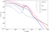 |
Fig. 1 Frequency-dependent opacity for the individual dust species. The solid line shows the total opacity (absorption + scattering), and the dotted line shows absorption alone. |
2.2 Temperature transition TΔ and 
To stabilize the solution of the combined radiative transfer and hydrostatic models, we need to prevent steep gradients. These can occur in either the accretion stress-to-pressure ratio, α (see Eq. (3)) or the dust-to-gas mass ratio,  (see Eq. (12)). A composition of only submicron silicate grains would sublimate over a short temperature range, usually shorter than what we could model with a grid capturing the whole disk. Solution to resolve the steep drop of the dust density at the silicate sublimation involves multiple grain sizes (Kama et al. 2009), static mesh refinement of the dust rim (Vinković 2012), dust diffusion (Schobert & Peeters 2021), or numerical smoothing (Flock et al. 2016). Models using a numerical smoothing with a single dust species without diffusion needed a smoothing of TΔ = 100 K, which was used by (Flock et al. 2016; Schobert et al. 2019; Flock et al. 2019; Chrenko et al. 2024). Including multiple dust species has the advantage of reducing the value of TΔ if needed, as the different sublimation temperatures of the dust species broaden the region over which the stellar irradiation is absorbed.
Another transition happens for the accretion stress-to-pressure ratio due to the transition between a highly turbulent and a low-turbulent state of the disk. This transition at the inner dead-zone edge mainly depends on the dust microphysics, the temperature, the magnetic field, and the external radiation (Desch & Turner 2015; Williams & Mohanty 2025). With a similar argument as before, previous works included a temperature transition to stabilize their models, while here models allowed a wider spread of values, from  K used by Flock et al. (2016); Schobert et al. (2019) to 70 K by Chrenko et al. (2024) to 25 K by Flock et al. (2019). In this work, we decided to use for most of the models the same temperature transition for both the α transition and the dust sublimation and set
  . In our reference model, we use TΔ = 100 K while we also present models for a steeper dust sublimation temperature range TΔ = 50 K.
2.3 Opacity
The wavelength-dependent opacities are generated with the Optool1 package for the different dust family species; see Table B.1. The frequency-dependent opacities, absorption, and total opacity per gram of dust are shown in Fig. 1. The frequency-dependent absorption opacity is used to determine the irradiation heating2. The irradiation flux is determined as
 (13)
(13)
with the Planck function B(νf, T∗), the solid angle Ωs, the surface temperature of the star T∗, the radius of the star R∗, the frequency νf, and the radial optical depth
 (14)
(14)
For the region between R∗ and the first cell in our domain, we take the gas opacity into account as the dust is fully sublimated. To determine the total absorption opacity in each cell, we sum the individual dust components  with λ = c/νf. The gas opacity is set to the low value of κgas = 10−6cm2/g and is constant along temperature and wavelength.
We generated mean Planck κP(T) and Rosseland’s opacities κR(T) from the wavelength-dependent opacities for the three dust family species, dependent on the local temperature. We note that we use the same silicate opacity for forsterite and enstatite. We include the total extinction opacity to determine the Rosseland opacity. To determine the total Planck and Rosseland opacity in each cell, we sum again over each dust component using  . More information on the opacity calculation can be found in Appendix B.
2.4 Model setup
We highlight again that compared to our previous models by Flock et al. (2019), we improve our models by three significant changes: (1) including frequency-dependent irradiation, (2) adding multiple dust species at different sublimation temperatures, and (3) adding large-scale magnetic fields. The first two main changes help to resolve the dust rim from a numerical point of view, and we do not need additional smoothing to avoid a sudden increase in ∆τr. This is because the location for radial optical depth unity τr(λ) = 1 differs for each wavelength, which broadens the layer where most of the irradiation heating is taking place. Also, the various dust components sublimate at different radii, smoothing out the radial profile of the total fD2G and so avoiding a sudden jump of dust density as is the case using a single dust species. We tested Eq. (12) for different resolutions in Appendix D to show convergence. Further discussion and alternative solutions for a single dust component of fD2G can be found in Flock et al. (2016) (Eq. (10)), Flock et al. (2019) (Eq. (9)), or Schobert & Peeters (2021) (Eq. (4)), which uses dust diffusion to smooth out the rim.
The final disk model is reached by iteratively solving for the radiation equilibrium solution and magnetohydrostatic equilibrium, including frequency-dependent irradiation from the star. Another difference to our previous model by Flock et al. (2016) and Flock et al. (2019) is that we use a cold boundary3 when determining the value of the radiation energy density in the ghost cells at the meridional boundary. However, we note that it remains difficult to argue what the correct boundary condition is (read more in the appendix of Chrenko et al. (2024). Our new models use a fixed temperature of 10 K within the ghost cells. Table 2 summarizes the model input parameters.
We follow previously established parameters of the radiative hydrodynamical models by Flock et al. (2016), model LS21, which should represent a class of Herbig-type stars used to derive a median SED by Mulders & Dominik (2012). For the ionization transition TMRI, we assume 900 K, which is set by thermionic emission of dust grains (Desch & Turner 2015). The accretion rate is constant over radius at 10−8 M⊙/yr. Compared to our previous models, we extend the domain to 100 au to capture the whole near and mid-IR emitting region of protoplanetary disks. The turbulent stress-to-pressure ratio is set to αMRI = 0.1 and αDZ = 0.001 which follows the results obtained from 3D radiation magnetohydrodynamic (MHD) simulations of the inner rim with a vertical magnetic field (Flock et al. 2017). To generate the initial conditions, we use a resolution of 2304 cells in radius with logarithmically increasing cell size and 216 cells in the meridional direction with uniform spacing for a domain extent from 0.1 to 100 au in radius and ∆θ = 0.6 rad (~34°). The inner domain boundary was chosen to reach hot enough temperatures so that the corundum dust component fully sublimates. For the different models, we vary the magnetic field strength, starting with a low value of Bz = 10 mG at 1 au, corresponding to a plasma beta (β = 2P/B2) of 2.26 × 10⁶ at the midplane after the radiation magnetohydrostatic equilibrium is reached for model M001. We increase the magnetic field strength successively until reaching a field strength of Bz = 0.3 G in the model M03 corresponding to a plasma beta of 2.51 × 10³. Following magnetic wind-driven accretion models, Bai & Goodman (2009) predict a minimum magnetic field of 0.1 Gauss to sustain an accretion rate of 10−8 M⊙/yr in the dead-zone, which would correspond to model M01. A similar magnetic field strength, corresponding to a plasma beta value of around β = 104, was also found by Lesur (2021) to be sufficient to sustain these accretion rates by a magnetically driven wind. Even stronger magnetized models are presented in Appendix E, reaching the maximum Bz = 3 Gauss in model M3.
Setup parameters for the disk models.
3 Results
We first show the results of our reference model M001. The radial surface density profiles of the gas and dust of model M001 are shown in Fig. 2, top. As shown in our previous works, the rise in the gas surface density becomes visible due to decreased accretion stress in the dead zone (Flock et al. 2016, 2019). Due to thermionic emission, the disk remains long enough ionized for the MRI to operate (Desch & Turner 2015), and the surface density rises beyond, but still close to, the dust sublimation front, around 0.34 au.
As shown in our previous models, due to the rise in surface density, there is a clear pressure maximum and a corresponding trap of solid material located at around 0.62 au, indicated with a dotted black line in Fig. 2, bottom. The temperature reaches 763 K at this dust trap with the disk aspect ratio H/R of 0.036. Fig. 2, top, also shows that the corundum grains survive the closest to the star, but only contribute a tiny fraction to the total dust surface density. Iron, forsterite, and enstatite show nearly the same sublimation region at 0.35 au. Only the corundum sublimates inward at 0.3 au.
The radial profiles of midplane temperature and aspect ratio H/R are shown in Fig. 2, bottom. The first substantial temperature drop happens at around 0.34 au due to the sudden dust condensation. A shallow drop in temperature then follows, which is caused by the curved rim, which changes the flaring and, therefore, the grazing angle of incoming irradiation at the disk surface between 0.4 and 1 au. The next steeper temperature drops happen between 1 and 3 au. Here, the accretion heating efficiency drops, which leads to a steeper drop in the temperature. There are two shadowed regions at 10 and 20 au, which can be seen in the H/R profile. In a shadowed region, the H/R remains constant over radius. In our models, these shadowed locations converge and do not propagate inward between the final iteration steps. In general, disk shadowing events were reported in previous works as well (Wu & Lithwick 2021; Ueda et al. 2021; Melon Fuksman & Klahr 2022; Kutra et al. 2024), and more dynamical simulations are needed to study their effect on the disk structure in the future.
Fig. 3 shows the 2D temperature and density structure of model M001. The temperature structure and the rim look broader and smoother compared to our previous model LS21 by Flock et al. (2016). We observe a hot dust halo in front of the rim. There is a round rim shape at which the temperature suddenly drops. Another main difference is the contribution of accretion heating, which results in the midplane being warmer than the layers below the irradiation absorption between 1 au and 3 au. There is a small shadowed region between 1 and 3 au and a flared disk beyond 3 au. For the reference model M001, the vertical magnetic field strength is 10 mG at 1 au. In the next subsection, we describe in more detail the influence of the magnetic field on the inner rim structure. The dotted green line shows the location where magnetic pressure equals thermal pressure. For model M001, the plasma beta unity line lies above the irradiation surface and in the optical thin layer. Due to the accretion heating, the snow line curves vertically and extends beyond 10 au in the midplane region, while in the disk atmosphere, it reaches further inward. To illustrate the snow line, we follow our previous routine by Flock et al. (2019) using the formula by Oka et al. (2011), which determines the water vapor mol fraction
 (15)
(15)
with the saturated vapor pressure
 (16)
(16)
We then determined the position where half of the water is in the form of ice by xice = 0.5 with
 (17)
(17)
Figure 3, bottom, presents the corresponding 2D gas density profile. The gas density is highest at the midplane at around 0.1 and 1 au, following the surface density profile. The H/R variations connected to the shadowing also become visible in gas density variations, especially in the upper layers. This can be seen best by looking at the pathway of the plasma beta unity line (dotted green line), which shows a jump between 1 and 3 au. In Fig. 3, we also show the sublimation of the corundum with the dotted magenta line. The steep temperature drop happens slightly radially outward compared to the dotted magenta line, which is because corundum condenses at small abundances that do not suffice to make the disk optically thick to stellar irradiation. The corundum thus contributes to the hot, optically thin emission. Fig. 3 also shows where the maximum of irradiation heating occurs (blue line), which is similar to the stellar spectrum weighted τr = 1 line. At the same time, the vertical rise of the line illustrates the grazing angle of the irradiation. The yellow and dotted orange lines trace the τz = 1 at 2.2 and 10 μm, which are almost tracing the identical disk surface and are both located below the τr = 1 line. To trace the midplane region, longer wavelengths are required (see the white separated dots, which trace the τz = 1 at 1 mm).
To disentangle the spatial distribution of various grain species, we show the corresponding 2D profile of corundum and iron dust grains in Fig. 4. The figure shows that a small amount of corundum survives in front of the inner rim due to the higher sublimation temperature than iron and the silicate group. The corundum grains constitute the heated dust halo before the rim. In contrast, the iron density shows a sudden and sharp drop at the rim. The sublimation temperature of iron is very close to enstatite and forsterite (see Appendix B). In both Figs. 3 and 4, we indicate the maximum pressure with a white circle at the midplane. In the following two sections, we introduce models with nearly no magnetization (β = 1.52 · 1010), with and without multi-grain species, and with different levels of TΔ to better distinguish their effect on the rim shape.
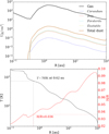 |
Fig. 2 Top: Surface density profile of model M001. The gas is shown in black, and the dust species are shown in color. Bottom: Midplane temperature profile (black) and H/R profile (red). The dotted line marks the position and corresponding temperature at the dust trap for which we would expect a substantial concentration of larger dust pebbles. |
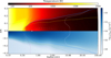 |
Fig. 3 2D temperature and gas density profile of model M001. The dotted green line shows plasma beta unity. The dotted black line shows the MRI transition (900 K contour line). The circle indicates the location of the pressure maxima where inward drifting pebbles can be trapped. The dotted magenta line shows the sublimation of the corundum. The solid white line shows the water snow line. The blue line shows the location of maximum irradiation heating corresponding to the τr = 1 line. The small yellow and orange dashes show the τz = 1 line at 2.2 and 10 μm (K and N bands). The small separated white dashes show the τz = 1 for 1 mm emission. |
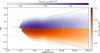 |
Fig. 4 2D dust density profile of model M001 for corundum (upper half) and iron (lower half). A small amount of corundum survives as a hot optically thin halo in front of the inner rim (τr = 1 blue contour). |
3.1 Rim shape and width
To study the effect of multiple dust species on the rim shape, we created two models with only one dust component, with and nearly without magnetic fields, model M001_S and model MZ_S. These models use the same total dust-to-gas mass ratio, given in Table 1, and assume only a single silicate species represented by forsterite. The results are summarized in Fig. 5 and Table 3. We measure the size and extent of the inner rim by determining the innermost location in the disk where τz = 1 and the outermost location where the temperature drops below 800 K at τi = 1 (Flock et al. 2016). Further, we determine the height of this location. Both pure silicate models M001_S and MZ_S show a compact inner rim, starting at 0.42 au with a 0.12 au extent reaching the outer rim. The different levels of magnetization show no effect on the position or extent of the rim, which is expected as here the thermal pressure dominates by many orders of magnitude. Adding multiple dust species makes the rim rounder and smoother. For model MZ, the inner rim moves inward, starting at 0.33 au with an extent of 0.19 au. The normalized ring width for the multi-dust species model  is 0.58 compared to 0.28 for the pure silicate models MZ_S and M001_S. A larger normalized ring width seemed to be what is observed when looking at K-band observations with the VLTI (see Fig. 3, left in GRAVITY Collaboration (2019)).
As reported in Section 2.2, the temperature range TΔ which controls the transition between the MRI turbulent inner disk and the more laminar outer disk at TMRI can influence the rim structure. To distinguish the effect of this transition region, we created model MZ_TD50, which uses a transition temperature of TΔ = 50 K. The effect can be seen in Fig. 5, bottom. The rim surface becomes slightly steeper compared to the reference models with ∆T = 100 K, shifting the rim a little bit outward from 0.33 au to 0.36 au and ∆Rrim from 0.19 au to 0.2 au. At the same time, the height of the rim is increased here as well, from ∆θ = 0.085 above the midplane to ∆θ = 0.093.
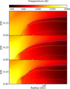 |
Fig. 5 Models with a very low magnetic field, zoomed into the temperature structure at the inner dust rim. From top to bottom: Model MZ_S with a single dust species, and models MZ and MZ_TD50 with multiple dust species. Model MZ_TD50 uses a steeper transition to change from αMRI to αDZ. The line styles are the same as in Fig. 3. |
Overview of the magnetized disk models.
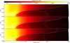 |
Fig. 6 2D temperature profile with increasing magnetization from top to bottom, showing models M001, M01, and M03. The dotted green line shows the plasma beta unity line. The blue line shows the location of maximal irradiation heating corresponding to the τr = 1 line. Using the local Planck opacity, the dotted yellow line shows the τz = 1 line. The solid white line shows the water snow line. |
3.2 Effect of magnetization
To study the effect of different magnetic fields, we show the 2D temperature profiles of the models with higher magnetization. Fig. 6 shows the different models with increasing magnetization from top to bottom. M001 and M01 are shown in the first and second row. The magnetization increases, which becomes visible in the shift of the plasma beta unity line closer to the midplane; see the dotted green line. The overall shape and extent of the inner rim are similar for all three levels of magnetizations (see Table 3). For higher magnetization, the disk becomes more puffed up, and the higher density leads to an extended heated dust halo inside the inner rim (compare temperature at R = 0.2 au and Z/R = 0.2 for different magnetized models in Fig. 6). Furthermore, higher magnetization reduces the grazing angle in the outer disk (beyond 3 au). Therefore, we observe that the ice line moves inwards, both at the midplane and the upper layers. At the midplane, the reduced density due to the larger vertical height leads to a reduction of the viscous heating. In the upper layers, two effects reduce the temperature and move the ice line inwards. First, the overall higher density leads to a higher optical depth, and so a reduction of the temperature in the disk atmosphere (above the τr = 1 line), and second, the grazing angle becomes reduced and so reduces the efficiency of irradiation absorption which can be seen by looking at the rise in the height of the blue line at around 10 au in Fig. 6. This reduction of the grazing angle is visible beyond 4 au in our models, radially inwards, the magnetic fields lead to an increase of the grazing angle due to the magnetic pressure support. We show the maximum heating by irradiation with the blue contour line, corresponding to the location of τr = 1. We determine the height at 1 au of this location to Z = 0.144 au for model M001 and M01. For model M03, we measure an increase to Z = 0.146 au. Our results show that the influence of moderate magnetic field strength becomes larger for the outer disk regions beyond 1 au, affecting the grazing angle of stellar starlight and so the disk flaring. The influence on the disk regions inside 1 au and in particular around the dust rim and the emitting region of the K-band emission remains small, as here the thermal pressure is much larger than the magnetic pressure.
Setup parameter for RADMC-3D.
4 Radiative transfer post-processing
In the following section, we post-process the dataset with the Monte-Carlo radiative transfer code RADMC-3D4 by Dullemond et al. (2012). The input parameters are summarized in Table 4. We first recalculate the dust temperature with RADMC-3D with the mctherm command using the 2D density of all four dust species. We ignore the gas opacity for this step. Here, we allow the individual dust species’ temperatures to decouple and assume isotropic scattering. In the second step, we calculate the images and the spectrum at different wavelengths.
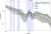 |
Fig. 7 SED for the different magnetized models from M001 to M03 calculated at 64 wavelengths (dots). The solid black line (crosses) and gray shaded color show the median SED and one-sigma error constructed by Mulders & Dominik (2012). All values shown here were normalized to a distance of 100 pc. |
4.1 SED comparison
In this subsection, we determine the SED for the individual magnetizations and compare it with the median SED, constructed by Mulders & Dominik (2012). The median SED comes with an upper and lower quartile information, telling us the range around the median where 50% of all flux values lie. We can use it to understand if our model represents a typical Herbig system or rather an outlier. Similar median SEDs were constructed for T Tauri stars (Furlan et al. 2006). The spectrum for the different magnetized models is shown in Fig. 7. The low and moderate magnetized models M001 and M01 show very similar SEDs even though model M01 has a midplane plasma beta with a factor 100 higher with βz = 2.29 × 10⁻⁴ at 1 au. As shown in Fig. 6, this can be explained by looking at the position of the β = 1 line, which lies above or close to the τr = 1 line. Here, the magnetization only affects the uppermost, low-density, and optically thin layers of the disk and so does not affect the temperature structure or the overall shape of the SED. Even though we did not fine-tune the model, the profile of the low- and moderate-magnetization models compares well with the median SED, mainly staying within the one-sigma deviations. The 10-µm feature in the median SED appears stronger than for our models and choice of opacity (comparing the flux ratio between 6 and 10 µm). This might indicate that our models are too optically thick, especially in the dead zone region, just outside the dust rim. Further, the H and K bands still show missing flux, similar to our previous work (Flock et al. 2016). The hot corundum grains that survive higher temperatures contribute to hot optically thin emission; however, the SED profile shows this contribution is insufficient. In the H band, the median flux is 1.7 times higher than the low magnetization models M001 and M01. In the N band at the peak of the silicate feature, the total flux of the low magnetized models matches very well with the median SED. At the same time, in the far-IR at 58 µm, the low magnetization models overshoot the emission flux by around two. For the higher magnetized model M03 with a midplane βz = 2.51 × 10³ at 1 au, the SED shows a clear increase of emission flux between the K and N bands. The increase in emission flux in the K band brings model M03 SED closer to the median SED. However, the model emission flux between 6 to 10 µm moves away from the median value. Overall, we think model M03 is less comparable to the median SED. The magnetic pressure increases the disk surface, affecting the stellar absorption layer, as shown in the previous section. The results of model M03 should be interpreted with care, as we would expect strong magnetic torques at the magnetic wind base for model M03, leading to a reduction of the surface density and so a change in the overall structure.
Comparison to the near-IR interferometry constraints of observed systems.
4.2 H-band comparison
First, we focus on the H-band observations with PIONIER/VLTI of Herbig type stars by Lazareff et al. (2017). As we have seen from the comparison to the median SED, our models still miss flux in the H band. The observations described in Lazareff et al. (2017) measured the fraction of H-band emission flux, which comes from the disk, and the radial position, where half of the emission is coming from. The half-light radii are the results of parametric fitting, and Chrenko et al. (2024) showed that this result can be used as a robust observational constraint. We chose observations of three Herbig stars with similar stellar luminosities to our model. The results are summarized in Table 5. We note that we used the distances from the Gaia DR3 release. The errors in the table are taken directly from the individual measurements of the different publications. What becomes directly visible is that the half-light radius in the H band of the three objects lies systematically inward compared to our models. HD 163296 and HD 100546 show similar positions, with 0.22 ± 0.05 au and 0.26 ± 0.01 au. HD 169142 has a half-light radius in the H band of 0.11 ± 0.02 au5, while an independent measurement with the Center for High Angular Resolution Astronomy (CHARA) long-baseline interferometer shows a best fit of 0.21 ± 0.01 au (Setterholm et al. 2018). For our fiducial model M001, we determined the H-band half-light radius to 0.31 au, while the higher magnetization model shows even a slight increase to 0.34 au for model M03. This comparison shows that most of the missing H-band flux should come from inside the silicate dust rim. Although we include corundum grains in our models, which survive close to the star at higher temperatures, they only slightly increase the H-band flux. The discussion section will outline some possible physical processes that could cause the additional compact emission. Further, we can compare the disk H-band emission fraction to the stellar contribution. For the models, we determine the H-band emission fraction from the disk by using the emission flux from our model domain starting at 0.1 au. From the VLTI observations, this is done by fitting three components to the visibility profile: an unresolved stellar component that manifests as a plateau at longer baselines, resolved disk emission at shorter baselines, and extended emission. Extended emission in the H band could be caused by scattered starlight, but the previous observations of these three objects reported strong vari-ations6. In our models, roughly one-third of the emission in the H band comes from the disk. We determine a fraction of 0.28 of disk H-band emission for the model M001, increasing to 0.3 for model M03. For the selection of Herbig systems, the values are diverse, from 0.76 ± 0.01 for HD 163296, to 0.42 ± 0.02 in HD 100546, until 0.17 ± 0.01 in HD 169142. This also shows that at least the two specific systems follow the trend we saw for the median SED comparison: the overall flux in the H band coming from the disk is higher than in our models. One might think no IR excess is needed to describe the H-band flux for the system HD 169142 due to the low fraction of disk emission in the H band. However, previous works also needed to add hot dust emission at 1800 K to fit the H-band emission (Tschudi & Schmid 2021).
4.3 K-band comparison
For the K-band comparison, we focus on the observations and data obtained with GRAVITY/VLTI by GRAVITY Collaboration (2019). All three objects show very similar K-band half-light radii, with 0.33 ± 0.07 au for HD 169142, over 0.3 ± 0.01 au for HD 163296 to 0.28 ± 0.01 au for HD 100546. These results match our fiducial model M001, which has a halflight radius of 0.34 au. The higher magnetized models show values of 0.42 au for model M03, less comparable to the observations. Here, the larger radius is an effect of the higher K band emission at larger radii (see Section 4.5). The spread in the fraction of disk emission between the three observed objects is smaller in the K band compared to the H band, with 0.81 ± 0.01 for HD 163296 to 0.63 ± 0.01 for HD 100546 until 0.4 ± 0.05 for HD 169142 again the lowest fraction as it was seen in the H band7. Our models show a fraction of disk K-band emission ranging from 0.46 for model M001 to 0.51 in model M03. Overall, the fraction of disk emission in the K band is still higher in the observed disks than in our models, except for the system HD 169142, which shows a value similar to model M001. This is consistent with the median SED showing a higher K-band flux than our models. We summarize: the K-band half-light radius matches our models better, especially for the low magnetized models, which could indicate that the shape, position, and dust temperature could represent the observed systems. Still, an additional hot emission component is needed within the dust rim to explain the H-band half-light radius and the total flux in both H and K bands.
4.4 N-band comparison
We focus on the observations taken with MIDI/VLTI by Menu et al. (2015) for the N-band comparison. In the MIDI N band, the observations recovered the total flux and the half-light radius. We normalized the total flux to a distance of 100 pc as we did for the median SED. One quickly notices a much larger spread in the N-band emission for our selection of the three Herbig-type systems compared to our models. HD 100546 has the largest N-band flux, with 69.1 ± 1.5 Jy and a half-light radius of 21.3 ± 1.1 au. In contrast, HD 163296 shows a half-light radius of 0.82 ± 0.05 au and a flux of 16.3 ± 0.6 Jy. Further HD 169142 shows only a flux of 0.92 ± 0.26 Jy with a half-light radius of 9.5 ± 2.3 au. For all our models, the N-band half-light radius remains inside 1 au, ranging from 0.79 au for model M001 to 0.93 au for model M03. As previously reported, the magnetic fields affect mostly the mid-IR flux, including the N-band flux. We obtain a flux of 25.7 Jy for model M001 in the N band, which increases for higher magnetization to 36.2 Jy for model M03. Finally, we note again that the median SED showed a total N-band flux of 28 ± 15 Jy, which compares very well to our fiducial model. The comparison shows that the system HD 163296 best fits our model and the median SED. Given the large deviations for the N band results for the systems HD 100546 and HD 169142, we believe that these systems could be more complex, for instance, either being a circumbinary disk or having a dust-depleted inner disk. Menu et al. (2015) also argue that both systems HD 100546 and HD 169142 have wide dust gaps affecting their N-band emission.
We conclude the last two subsections by showing Fig. 8, which summarizes the results in the K and N bands and compares the observations. The system HD 169142 (black cuboid) shows the largest error in the K-band half-light radius, still comparing well with the K-band half-light radius of our models. This system shows the lowest N-band emission (color), which might be a combination of having a low accretion rate and the inner disk regions being depleted in dust or shadowed, indicated by the large half-light radius of ≈9.5 au in the N band. The system HD 100546 (yellow cuboid), in contrast, has a relatively high accretion rate and shows the highest N-band flux, together with a colossal N-band half-light radius of ≈21.3 au, indicating a dust-depleted inner disk region. The errors in the H and K bands are minimal, with the K-band radius also being close to the values from our models. The system HD 163296 (dark blue cuboid – top left), with a similar accretion rate as HD 100546, compares best to our models. The half-light radius in the K band (≈0.3 au), the N-band half-light radius (≈0.82 au), and the total N-band flux (≈16 Jy) are very close to our models, especially the low magnetized model M001.
4.5 H-band emission and effect of accretion heating
In our new models, we have shown that adding multiple grain species with realistic sublimation temperatures and abundance makes the rim smoother. However, even though corundum grains survive at higher temperatures, they do not increase the H-band flux. On the contrary, the H-band flux decreases, as the rim becomes broader and smoother. The effect is shown in the top panel of Fig. 9. The dotted green line shows that a more compact and less smooth rim helps in increasing the H and K-band flux. Having only silicate grains, the H-band flux increases as the rim becomes less smooth and more wall-like. We added one additional model M001_S_TC, similar to Chrenko et al. (2024), to include a single dust component with a constant condensation temperature of 1550 K. This configuration leads to a more compact and hotter dust rim. A more wall-like structure like this was also recommended by Chrenko et al. (2024) to fit the visibility curves for HD 163296 better. For this model M001_S_TC, the SED profile looks very similar to the median SED; compare the blue line in Fig. 9, top. When comparing the half-light radius model M001_S_TC can only fit the H-band half-light radius with aH = 0.24, which compares well with the systems HD 163296 and HD 100546. However, the half-light radius of the K band remains too small compared to observations. We, therefore, conclude that a better fitting model would be similar to M001 with additional H-band flux of unknown origin without affecting the overall smooth rim structure much. In the discussion section, we present additional RADMC3D models that could produce this additional flux. The details of these pure silicate models can be found in Appendix C. In the previous subsections, we ignored the accretion heating in the RADMC3D models. To check the influence of the viscous heating onto the SED, we incorporate viscous heating into RADMC3D by using the local αheat to calculate the internal heating using the heatsource.inp file. Here, we implement a fixed α heating profile depending on the radius using
![Mathematical equation: \alpha_\mathrm{heat}=\frac{1}{2} ( \alpha_\mathrm{MRI} - \alpha_\mathrm{DZ}) \left [ 1.0 - \tanh \left ( \frac{r-0.3\, \mathrm{au}}{0.1\, \mathrm{au}} \right ) \right ] + \alpha_\mathrm{DZ}](/articles/aa/full_html/2025/09/aa53124-24/aa53124-24-eq41.png) (18)
(18)
to also capture the stronger heating inwards the dust rim expected by the MRI. The value of 0.3 au was chosen to represent the MRI transition of the reference model. The profile is static to prevent any dynamic feedback. The transition range was chosen here over 0.1 au. A model SED with viscous heating like this is shown in Fig. 9 (see the dashed red line). There is nearly no difference compared to the passive model, with only a slight increase in the flux between 5 and 20 µm. For instance, we see an 8% flux increase with accretion heating at 10 µm. This can be explained by accretion heating, which increases only the midplane temperature. It does not strongly affect the temperature layer directly below the irradiation absorption, which contributes most to the near-IR emission. Further, the MRI heated, dust-free, optical thin regime contributes only a little to the total flux (see Fig. 9, bottom).
The radial intensity profile at the K band is shown in Fig. 9, bottom. The intensity peak is emitted from the “nose” of the dust rim, located at the midplane and around 0.35 au for most models. The accretion heating increases the emission inside the rim (see Fig. 9, bottom) but not strong enough to change the total flux (see Fig. 9, top). The profile remains very similar to the passively heated model. The radial intensity profile of the higher magnetized model M03 shows that the flux increase comes from the region radially outward 0.6 au, which can be explained by the slightly puffed-up surface for irradiation absorption. For the model M001_S_TC the emission is more compact and overall higher due to the higher temperature of the “wall-like” rim.
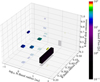 |
Fig. 8 Visualizing the entries in Table 5. For the observed disks, the position and size of the block size represent the corresponding value and error. For the model entries, we set a constant block size (the three equally sized blocks). The color of the block represents the N-band flux normalized at 100 pc for each object and model. |
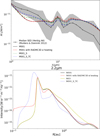 |
Fig. 9 Top: SED for additional models with accretion heating (red dashed), with silicate grains alone (dotted green), and with silicates with a constant and high (Tev = 1550 K) sublimation temperature M001_S_TC (dotted blue). The red dashed line was calculated based on model M001, including accretion heating in the RADMC3D calculation. Bottom: radial intensity profile along the major axis (Y=0) for models M001, M03, M001 with accretion heating in RADMC3D and model M001_S_TC in the K band (2.2 µm). |
4.6 Synthetic images in the K, L, and N bands
The 2D images, calculated with an inclination of 45 degrees in the K L, and N bands, are summarized in Fig. 10. The low and moderate magnetization models M001 and M03 show very similar emission profiles in the K and L bands. They show the peak emission from a narrow ring with a broader, less intense outer ring. In the N band, model M03 shows a more extended emission area due to the small changes in the flaring angle. For comparison, we also show the model M001_S_TS with one dust component and a fine-tuned dust sublimation temperature independent of the local pressure. This model image shows a more compact, broader, and brighter ring of emission. In Appendix E, we show further an image for the very magnetized model M3.
4.7 Toy model to account for the emission deficit by adding hot dust emission
In this section, we present two additional RADMC3D models. The goal here was to boost the H-band emission without changing the physical structure of our models. In the first model, we added a small amount of corundum dust to mimic more dust material inside the rim. We added a flat value of the dust to gas mass ratio to the corundum dust density times the gas density 10−8ρ. This should mimic an optically thin dust halo surrounding the disk. For this dust halo, we neglected dust sublimation for these extra grains. The SED profile of this “dust halo” RADMC3D model is shown in Fig. 11, dotted blue line. The H- and K-band emission increases due to the higher emission of hot material; however, it still cannot explain the observed values.
For the second model, we assumed emission from compact evaporating planetesimals with a surface temperature of 1800 K, a circular emitting area with a radius of 0.0733 au. The choice of the temperature is motivated by the highest refractory material sublimation temperature. The choice of the area was arbitrary and set to match the emission at 2 µm. As we would expect large tails of hot dust emission due to the planetesimals’ evaporation, it is not easy to estimate the amount and mass of planetesimal material that could cause this emission. We expected the evaporation tail, and therefore the emitting area, to be several orders of magnitude larger than the planetesimal’s area itself (Biermann 1963). For this “evaporating objects” model, we added a point source of stellar emission in the stars.inp file of the RADMC3D setup. The exact position is at the center in the X–Y plane and in the Z-direction 0.015 au above the central star, which is a constraint for the current axisymmetric setup and version of RADMC3D. We show and compare the SED profile in Fig. 11, green dashed line. The “evaporating objects” model, which assumed an additional continuum source to mimic evaporating planetesimals, can match the H- and K-band emission flux well. We note that both models require fine-tuning. The extra dust is fine-tuned as it cannot be too large, as it otherwise becomes optically thick for the irradiation, which reduces the temperature in the inner regions. For the small objects model, we needed to fine-tune the area to match the emission.
5 Discussion
5.1 Width of the α transition at the edge of the inner dead zone
One important property of the inner dead-zone edge is the steepness of the surface density rise. A steeper rise in surface density leads to larger outward migration torque onto planets trapped at this location (Masset et al. 2006; Flock et al. 2019; Chrenko et al. 2022). At the same time, the steepness of the surface density rise determines the strength of the radial pressure gradient and so the efficiency of concentrating pebbles (Izidoro et al. 2021). This steepness is determined by the drop of the MRI activity, which depends on the strengths of the nonideal diffusivity of Ohmic, Ambipolar, and Hall. As a guideline, Desch & Turner (2015) (see Fig. 17 for the midplane) showed that the Ohmic and Ambipolar Elsasser number increases from 0.1 to 1.0 between 900 K and 950 K, pointing to a transition of around 50 K. However, this depends on many parameters, like the strength of the magnetic field, the local ionization rate by radiation, the local gas and dust density, and the dust size (Delage et al. 2022). New models of ionization focusing on the inner disk Williams & Mohanty (2025) emphasize the importance of the grain size distribution, also showing a very steep drop in resistivity with temperature, but did not specify the Elsasser number. Global 3D radiation non-ideal MHD simulations also point to a very sharp drop in MRI activity (Flock et al. 2017) between 900 K and 1000 K, with an α drop by at least 2 orders of magnitude. We summarize that most of the works point to a very sharp ionization transition between 100 K and below, close to the resolution limit of current 2D or 3D radiation MHD models.
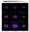 |
Fig. 10 2D intensity map calculated for an inclination of 45° in the K band (2.2 μm, top), L band (3.45 μm, middle), and N band (10 μm, bottom) using a linear color map and normalized over the individual peak intensity in units of W sr−1 m−2 Hz−1. From left to right: Models M001, M03, and M001_S_TS. |
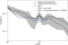 |
Fig. 11 Similar to Fig. 7, showing the SED for two additional models that include a dust halo (dotted blue line) and evaporating objects (dashed green line). The solid black line (crosses) and gray shading show the median SED and one-sigma error constructed by Mulders & Dominik (2012). All values shown here were normalized to a distance at 100 pc. |
5.2 Constraining the magnetic flux in the inner disk
With our models, one goal was to answer the question about the strength of the magnetic field in the inner disk based on the current observational constraints. The goal is based on the idea that the disk becomes more puffed-up due to magnetic pressure support, and so the thermal IR emission substantially increases. Our results show that this effect occurs at relatively strong magnetic field strengths for the models M03 and beyond, corresponding to plasma beta values of around ≈103. This substantial excess in emission is not seen in the median SED. We therefore argue that most of the observed young Herbig disks are weakly magnetized with beta values ⪆104. We remember the limitation of our models, especially for the strongly magnetized models in Appendix E. Dynamical simulations will here show a substantial increase in the accretion rate (Lesur et al. 2023), reducing the density and changing the temperature structure. Future models should include the magnetic torque and the corresponding accretion stress.
5.3 Location of the magnetic wind base
The wind base of the magnetic-driven wind can be approximated in our models with the τr = 1 layer as most of the far-UV radiation is absorbed close to this layer; see the blue line in Fig. 6. By comparing model M001 to model M03, we see that the magnetization at this location changes from a weakly magnetized case (β > 1) in model M001 to a stronger magnetized case (β < 1) in model M03 at this height. However, even with this change, the location in height for both τr = 1 and β = 1 remains close by, which explains that the resulting emission profiles are very similar. Our results show that as long as the far-UV or irradiation absorption layers remain below or close to the magnetized layer (β = 1 region), we would not expect a substantial change in the near-IR emission. However, we notice a stronger effect in the N-band emission, which is due to the change in the grazing angle. The increase in the N-band flux for higher magnetization was seen both in the images and in the total flux (see Table 5 and Fig. 10).
5.4 The nature of H-band emission and opacity sources inside the silicate sublimation
Our results show that including magnetization and multi-dust species affects the density and temperature structure. Although the IR flux increases for stronger magnetic fields, the results show that magnetic fields alone cannot explain the excess in the H-band flux. Turner et al. (2014) were able to find a better match to the observed H-band flux using a magnetically supported disk. However, they set the inner dust rim location by hand without including dust sublimation. Further, they used a density fit to model the effect of the magnetic field, and they modeled only one field strength. Their models also were overshooting the emission flux at around 6 to 7 µm, similar to our models with a field strength above Bz = 0.3 G at 1 au (see Appendix E).
Adding corundum grains makes the rim smoother and radially more extended, which has the opposite effect of a sharp wall and even reduces the flux in the H band (see Fig. 9). Another potential opacity source inside the silicate sublimation could come from graphite. In this work, we do not consider graphite grains, as several studies have pointed out that it is not the main carbon carrier in protoplanetary disks. Most carbon is supposed to be locked in amorphous carbon or PAH (Draine & Lee 1984; Serra Díaz-Cano & Jones 2008; Anderson et al. 2017). Furthermore, graphite is not included in the reference model of GGChem, which we choose for our model (see Woitke et al. 2018). They argue that most of the carbon is being lost at around 500 K at the soot line (see also Bergin et al. 2023). A recent work by Anderson et al. (2017) mentioned that refractory carbon might be destroyed before reaching the inner disk. However, we note that most of the works still focus on the main carbon carriers in amorphous grains and PAHs. Adding a small amount of graphite could lead to an optically thin heated layer, which would be an interesting study for the future.
Another source of opacity could come from various metal lines in the gas phase (Dullemond & Monnier 2010). By integrating over these lines with high spectral resolution Malygin et al. (2014) showed that metal lines in the gas phase can contribute significantly to the mean Planck opacity. This high opacity would block most of the stellar irradiation and shift the dust rim radially inwards. Realistic photochemistry (Kamp et al. 2017) and self-shielding rates might help to overcome this. In contrast, the Rosseland mean opacities are expected to remain small for the gas opacity, with values similar to those taken for this work (see more in Appendix B1 of Flock et al. (2019).
By fine-tuning and modifying the sublimation temperature and using a single dust component, we can almost match the H-band flux of the median SED and the H-band half-light radius (see also Chrenko et al. (2024). However, this tuned model is inconsistent with the observed K- and L-band half-light radius, and it ignores the sublimation temperature derived by GGchem. To match the H-band flux without affecting the rest of the disk structure of our reference model, we need an additional continuum component, which is geometrically thin and so does not block the irradiation onto the dust rim. Larger objects, for instance, a swarm of kilometer-sized evaporating objects on eccentric orbits, might be able to contribute an additional hot component.
6 Conclusion
We presented a new class of 2D radiative magnetohydrostatic multi-dust species disk models for protoplanetary disks. Our reference model followed a Herbig-type star-disk system with L* = 21L⊙ and a mass accretion rate of Ṁ = 1.0 × 10⁻⁸ M⊙/yr. The dust sublimation was determined using the code GGchem with solar abundance ratios for corundum, iron, forsterite, and enstatite grains at different temperatures and densities. The opacities were determined using the package Optool for each dust species. We implemented frequency-dependent irradiation, viscous heating, and the temperature-dependent Planck and Rosse-land opacities. By changing the strength of the magnetic field, we obtained several temperature and density profiles with different magnetization levels. By post-processing with a Monte Carlo radiative transfer, we determined the SED, the half-light radius in the H, K, and N bands, and the disk emission fraction for these wavelengths. We presented synthetic images and also compared our models to the results of detailed H-, K-, and N-band interferometric observations of systems HD 163296, HD 169142, and HD 100546 based on previous surveys by the PIO-NIER and GRAVITY instruments at the VLTI. Our key results are listed below:
The addition of multiple dust components with different sublimation temperatures broadens and smooths the inner dust rim. Corundum grains survive closer inside the inner rim and contribute as hot and optically thin dust emission in front of the dust rim. The optical thick rim starts at about 0.35 au for our choice of star and disk parameters. In our models, the magnetic fields mainly affect the upper layers in the disk in which magnetic pressure dominates. This increases the surface at which stellar irradiation is absorbed;
For our typical Herbig model, we observed a pressure bump at 0.62 au, which is an efficient trap for inward-drifting pebbles. The effect of including accretion heating and a temperature-dependent dust opacity varied the steepness of the temperature drop along the radius. These variations perturb the radial profile of H/R and resulted in several shadowed regions;
Based on the detailed comparison with observations in the H, K, and N bands, we found that magnetic field strengths of 0.1 Gauss at 1au and below fit the median SED best. These magnetic field strengths correspond to midplane plasma beta values of about 2 × 10⁴ and higher. This magnetic field strength is high enough to enable the mass accretion rate by magnetically driven winds in the model;
The effect of the magnetic fields increase when the plasma beta unity layer is less extended vertically than the irradiation layer (the height of the β = 1 line compared to the τr = 1 line). In contrast, the magnetic field strength of 0.3 Gauss and above at 1au emits more strongly in the mid-IR;
The observed H-band flux is still higher than in our models. Additional dust species make the rim smoother and so reduce the H-band emission compared to a single dust model with a steeper rim shape. Our results show that the magnetic pressure-supported atmosphere increases the emission in the mid-IR (3-9 μm) but less in the near-IR (≤2 μm), as most of the H-band flux is coming from a region near the midplane, which remains unaffected by magnetic fields;
The observed half-light radius of the H-band emission is closer to the star and inwards the dust rim. The observations show a half-light radius of aH ≤ 0.26 au while our models show aH ≥ 0.31. The results indicate that a geometrically thin, hot continuum emission is still missing. We are able to increase the H-band emission using an additional optical thin, non-sublimating dust component. We are able to match the H- and K-band emission of the median SED by fine-tuning the area of an additional compact emission at T = 1800 K, which should mimic a swarm of eccentric, larger evaporating objects inside the rim location;
The K-band half-light radius best fits our disk models, especially for low and moderate magnetization levels. Higher magnetization makes the K-band emission broader and shifts the half-light radius outwards. The total K-band flux from observations is also higher than our models, as in the case of the H band;
The N-band flux of 25.7 Jy for our low magnetized model matches best the median SED value. In contrast, we see a substantial spread in the N-band flux for the three specific disk systems, ranging over a factor of 75, with HD 169142 having the lowest value with 0.92 ± 0.26 Jy and HD 100546 the highest with 69.1 ± 1.5 Jy. The system HD 163296 best fits the low and moderate magnetization models when comparing K-band radius, N-band radius, and total N-band flux. With increasing magnetization, the N-band flux increases in our models, which might help to constrain disk magnetization in the future;
We find that the effect of viscous heating on the near and mid-IR emission remains low. The viscous heating mainly affects the midplane temperatures. While the water snow line is pushed outward, the temperature in the upper disk layers remains primarily unchanged. A viscously heated, MonteCarlo radiative transfer disk model shows an increase of N-band flux by only 8% compared to the passively heated disk model.
Finally, we find that very high magnetization levels change the disk’s structure to an envelope. In this case, the vertical density profile becomes flat due to the dominant magnetic pressure, and the temperature falls off with the radial distance to the star. Future work should perform such model cases in dynamical simulations to investigate the structure, which might be relevant for the very early phase of star and disk formation.
Acknowledgements
The authors thank Karine Perraut, Catherine Dougados, and Lucas Labadie for their discussions and feedback on interpreting the VLTI results during the YSO Gravity meeting in 2024. We also thank Jean-Philip Berger and John Monnier for their discussions and for interpreting the CHARA results. This research was supported in part by the grant NSF PHY-2309135 to the Kavli Institute for Theoretical Physics (KITP). M. F. has received funding from the European Research Council (ERC) under the European Union’s Horizon 2020 research and innovation program (grant agreement No. 757957). The work of O.C. was supported by the Czech Science Foundation (grant 21-23067M) and the Charles University Research Centre program (No. UNCE/24/SCI/005). T.U. acknowledges the support of the DFG-Grant, project number 465962023. J. V. is funded by the Hungarian NKFIH OTKA project no. K-132406 and no. K-147380. J. V. acknowledges support from the Fizeau Exchange Visitors program. The research leading to these results has received funding from the European Union’s Horizon 2020 research and innovation program under Grant Agreement 101004719 (ORP). This project has received funding from the European Research Council (ERC) under the European Union’s Horizon 2020 research and innovation program (PROTOPLANETS, grant agreement No. 101002188). This work was also supported by the NKFIH NKKP grant ADVANCED 149943 and the NKFIH excellence grant TKP2021-NKTA-64. Project no.149943 has been implemented with the support provided by the Ministry of Culture and Innovation of Hungary from the National Research, Development and Innovation Fund, financed under the NKKP ADVANCED funding scheme.
Appendix A Equations for the radiation magnetostatic case
In this section, we display the magnetohydrostatic equations, which are solved to derive the azimuthal velocity and the density structure. Using the corresponding divergence operator, we can determine  with
with
 (A.1)
(A.1)
and then do a half-cell integration to obtain the new density using
 (A.2)
(A.2)
The magnetic field remains fixed during all iteration steps.
Appendix B GGchem and Optool
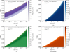 |
Fig. B.1 Dust species abundance in the density and temperature plane calculated with GGchem: corundum (a), iron (b), forsterite (c), and enstatite (d). The red lines show where 50% of the maximum abundance is reached. The dashed lines show the fitting function we derived and used for our models. |
For GGchem, we used the standard model using solar abundances, with equilibrium condensation and 1800 points in each direction of the 2D temperature and density regime (Woitke et al. 2018). We show the abundance of the different dust species derived in Fig. B.1. The fitting functions are summarized in Table 1 and Fig. B.2, left. The command to derive the corresponding dust opacities is summarized in Table B.1. The first command calculates the opacity for the two silicate dust grain groups. We follow the standard DIANA opacities (Woitke et al. 2016), which assume a specific pyroxene (70% Mg) and carbon in a mass ratio 0.87/0.13 and with a porosity of 25%. We assume a grain size distribution with grains between 0.05µm and 10µm with the typical grain size power law of a−3.5 . In our models, the DIANA opacities represent the opacity of the enstatite and forsterite, the two most significant mass fractions of the dust mass composition; see Table 5. The opacity for the corundum and iron are calculated using the same dust size distribution with a zero porosity level. Finally, we note that further improvements of the opacity are possible as the DIANA opacity is based on Mg0.7Fe0.3SiO3 plus carbon material, while forsterite (Mg2SiO4) and enstatite (MgSiO3) are purely composed of Mg, Si, and O. The temperature-dependent Rosseland and Planck mean opacities used for the model are shown in Fig. B.2, right. We also note that we assume three separate dust species when averaging the mean opacity in section 2.3 instead of forming a new complex grain species with multiple ingredients. By calculating with Optool for a grain mixture of Corundum, Iron, and Silicates, each with 33% mass fraction, we found an absorption opacity at 1 µm larger by around 67% compared to just averaging over the grain opacity of the three species with pure material composition. Determining the opacity in each cell for a specific mixture of dust species would require running Optool for each dust mixture in every cell, which would go beyond the scope of this work.
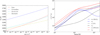 |
Fig. B.2 Left: Derived fitting functions of the sublimation temperature for the dust species. Right: Planck and Rosseland opacities dependent on temperature for the three groups of dust species. The Rosseland opacities were calculated using the total extinction opacity. |
Commands to generate the opacity using Optool.
Appendix C Pure silicate grains test
We explain here the model M001_S and M001_S_TS, which both have only one dust species. The total dust mass stays the same. However, we had to replace Eq. (12) with the previous formula used by Flock et al. (2019) to resolve the optical depth transition due to the steep rise in dust density. The other parameters and setup remain the same. The rim has a steeper and more considerable vertical extent, similar to that found in (Flock et al. 2016). Further, for model M001_S_TS, we fix the evaporation temperature to a constant temperature value of 1550 K without any density dependence. This leads to an even steeper wall, similar to that described in Chrenko et al. (2024).
Appendix D Resolution test
In this section, we test the convergence of the models. We especially want to test the new sublimation function (see Eq. (12)). We double the resolution of model M001, having 4608 cells in the radial direction and 432 in the θ direction. We compare the radial profile of the temperature and the density profiles of corundum and iron at the height of Z/R = 0.1 in Fig. D.1, left. The results are very similar and show convergence. An overview of the temperature profile from all models in Table 3 is shown in Fig. D.1, right.
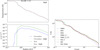 |
Fig. D.1 Convergence test for model M001 with double resolution. The profiles of temperature (top left) and dust densities (bottom left) remain very similar. Right: 1D midplane temperature profile for all models listed in Table 3. |
Appendix E Strongly magnetized models
Figure E.1 shows the temperature profiles for the models with very high magnetization; see Table E.1. Looking now at models M06 and M1 (first and second row), the ice-line continues to move inward due to the steeper temperature gradient caused by the higher density in the disk atmosphere. The disk becomes more similar to an optically thick envelope. By further increasing the magnetization in model M1 and M3, the disk becomes fully magnetically dominated with the plasma beta below unity inside 1.2 au. In the optical thick envelope, the stellar radiation is quickly absorbed. In model M3, the local density becomes so high that it becomes optically thick even close to the vertical boundary. Close to the vertical boundary, the temperature is affected by the boundary condition. The dust trap moves first inward, reaching 0.43 au for model M06 and then moves outward beyond 1 au for model M1 and M3 due to the combined effect of magnetic pressure and the drop in α. The magnetic-dominated atmosphere puffs the disk up, leading to a plateau and secondary ring in the K-band image; see Fig. E.2, left. The SED shows that the magnetized models show a strong excess at mid-IR wavelength, which is not seen in the median SED; see Fig. E.2, right. An apparent excess in emission between 3 to 10 µm is due to the modified density and temperature structure. This excess in the mid-IR was also reported in the work by Turner et al. (2014); see their Fig. 7. We obtained a slight increase in H- and K-band emission for the magnetized models; however, the overall shape of the SED does not match. As emphasized in the discussion section, the high-magnetized models have a limitation. Magnetic torques in the upper disk layers would lead to a strong accretion rate and, therefore, reduce the surface density substantially, so the overall structure in temperature and density would also change.
Overview of the strongly magnetized disk models.
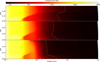 |
Fig. E.1 2D temperature profile with increasing magnetization from top to bottom showing models: M06,M1 and M3. The dotted green line shows the plasma beta unity line. |
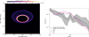 |
Fig. E.2 Left: 2D intensity map calculated for an inclination of 45° at 2.2 μm zoomed into the 1 au region shown for the very magnetized model M3. Right: SED for the high magnetized models from M06 to M3 showing the 64 calculated wavelength points (dots). The gray shaded color and solid black line show the median SED constructed by Mulders & Dominik (2012). All values were normalized to a distance at 100 pc. |
References
- Anderson, D. E., Bergin, E. A., Blake, G. A., et al. 2017, ApJ, 845, 13 [NASA ADS] [CrossRef] [Google Scholar]
- Bai, X.-N., & Goodman, J. 2009, ApJ, 701, 737 [NASA ADS] [CrossRef] [Google Scholar]
- Bans, A., & Königl, A. 2012, ApJ, 758, 100 [Google Scholar]
- Batalha, N. M., Rowe, J. F., Bryson, S. T., et al. 2013, ApJS, 204, 24 [Google Scholar]
- Bergin, E. A., Kempton, E. M. R., Hirschmann, M., et al. 2023, ApJ, 949, L17 [Google Scholar]
- Biermann, L. 1963, Space Sci. Rev., 1, 553 [Google Scholar]
- Bitsch, B., Crida, A., Morbidelli, A., Kley, W., & Dobbs-Dixon, I. 2013, A&A, 549, A124 [NASA ADS] [CrossRef] [EDP Sciences] [Google Scholar]
- Boley, A. C., Morris, M. A., & Ford, E. B. 2014, ApJ, 792, L27 [Google Scholar]
- Cecil, M., & Flock, M. 2024, A&A, 692, A171 [NASA ADS] [CrossRef] [EDP Sciences] [Google Scholar]
- Chatterjee, S., & Tan, J. C. 2014, ApJ, 780, 53 [Google Scholar]
- Chrenko, O., Chametla, R. O., Nesvorný, D., & Flock, M. 2022, A&A, 666, A63 [NASA ADS] [CrossRef] [EDP Sciences] [Google Scholar]
- Chrenko, O., Flock, M., Ueda, T., et al. 2024, AJ, 167, 124 [Google Scholar]
- Colavita, M. M., Wizinowich, P. L., Akeson, R. L., et al. 2013, PASP, 125, 1226 [Google Scholar]
- D’Angelo, G., & Bodenheimer, P. 2013, ApJ, 778, 77 [Google Scholar]
- Delage, T. N., Okuzumi, S., Flock, M., Pinilla, P., & Dzyurkevich, N. 2022, A&A, 658, A97 [NASA ADS] [CrossRef] [EDP Sciences] [Google Scholar]
- Desch, S. J., & Turner, N. J. 2015, ApJ, 811, 156 [NASA ADS] [CrossRef] [Google Scholar]
- Draine, B. T., & Lee, H. M. 1984, ApJ, 285, 89 [NASA ADS] [CrossRef] [Google Scholar]
- Dra˛z˙kowska, J., Bitsch, B., Lambrechts, M., et al. 2023, in Astronomical Society of the Pacific Conference Series, 534, Protostars and Planets VII, eds. S. Inutsuka, Y. Aikawa, T. Muto, K. Tomida, & M. Tamura, 717 [Google Scholar]
- Dullemond, C. P., & Monnier, J. D. 2010, ARA&A, 48, 205 [NASA ADS] [CrossRef] [Google Scholar]
- Dullemond, C. P., Dominik, C., & Natta, A. 2001, ApJ, 560, 957 [NASA ADS] [CrossRef] [Google Scholar]
- Dullemond, C. P., Juhasz, A., Pohl, A., et al. 2012, Astrophysics Source Code Library [record ascl:1202.015] [Google Scholar]
- Dzyurkevich, N., Flock, M., Turner, N. J., Klahr, H., & Henning, T. 2010, A&A, 515, A70 [NASA ADS] [CrossRef] [EDP Sciences] [Google Scholar]
- Fabrycky, D. C., Lissauer, J. J., Ragozzine, D., et al. 2014, ApJ, 790, 146 [Google Scholar]
- Flock, M., Fromang, S., González, M., & Commerçon, B. 2013, A&A, 560, A43 [NASA ADS] [CrossRef] [EDP Sciences] [Google Scholar]
- Flock, M., Fromang, S., Turner, N. J., & Benisty, M. 2016, ApJ, 827, 144 [CrossRef] [Google Scholar]
- Flock, M., Fromang, S., Turner, N. J., & Benisty, M. 2017, ApJ, 835, 230 [CrossRef] [Google Scholar]
- Flock, M., Turner, N. J., Mulders, G. D., et al. 2019, A&A, 630, A147 [NASA ADS] [CrossRef] [EDP Sciences] [Google Scholar]
- Furlan, E., Hartmann, L., Calvet, N., et al. 2006, ApJS, 165, 568 [CrossRef] [Google Scholar]
- Grady, C. A., Schneider, G., Hamaguchi, K., et al. 2007, ApJ, 665, 1391 [Google Scholar]
- GRAVITY Collaboration (Perraut, K., et al.) 2019, A&A, 632, A53 [NASA ADS] [CrossRef] [EDP Sciences] [Google Scholar]
- Hillenbrand, L. A., Strom, S. E., Vrba, F. J., & Keene, J. 1992, ApJ, 397, 613 [CrossRef] [Google Scholar]
- Ida, S., & Lin, D. N. C. 2010, ApJ, 719, 810 [Google Scholar]
- Izidoro, A., Ogihara, M., Raymond, S. N., et al. 2017, MNRAS, 470, 1750 [Google Scholar]
- Izidoro, A., Bitsch, B., & Dasgupta, R. 2021, ApJ, 915, 62 [NASA ADS] [CrossRef] [Google Scholar]
- Kama, M., Min, M., & Dominik, C. 2009, A&A, 506, 1199 [NASA ADS] [CrossRef] [EDP Sciences] [Google Scholar]
- Kamp, I., Thi, W. F., Woitke, P., et al. 2017, A&A, 607, A41 [NASA ADS] [CrossRef] [EDP Sciences] [Google Scholar]
- Kutra, T., Wu, Y., & Lithwick, Y. 2024, ApJ, 964, 165 [Google Scholar]
- Lazareff, B., Berger, J. P., Kluska, J., et al. 2017, A&A, 599, A85 [NASA ADS] [CrossRef] [EDP Sciences] [Google Scholar]
- Lesur, G., Flock, M., Ercolano, B., et al. 2023, in Astronomical Society of the Pacific Conference Series, 534, eds. S. Inutsuka, Y. Aikawa, T. Muto, K. Tomida, & M. Tamura, 465 [Google Scholar]
- Lesur, G. R. J. 2021, A&A, 650, A35 [NASA ADS] [CrossRef] [EDP Sciences] [Google Scholar]
- Levermore, C. D., & Pomraning, G. C. 1981, ApJ, 248, 321 [NASA ADS] [CrossRef] [Google Scholar]
- Lissauer, J. J., Ragozzine, D., Fabrycky, D. C., et al. 2011, ApJS, 197, 8 [Google Scholar]
- Lissauer, J. J., Dawson, R. I., & Tremaine, S. 2014, Nature, 513, 336 [Google Scholar]
- Malygin, M. G., Kuiper, R., Klahr, H., Dullemond, C. P., & Henning, T. 2014, A&A, 568, A91 [NASA ADS] [CrossRef] [EDP Sciences] [Google Scholar]
- Marleau, G.-D., Mordasini, C., & Kuiper, R. 2019, ApJ, 881, 144 [Google Scholar]
- Masset, F. S., Morbidelli, A., Crida, A., & Ferreira, J. 2006, ApJ, 642, 478 [Google Scholar]
- Melon Fuksman, J. D., & Klahr, H. 2022, ApJ, 936, 16 [NASA ADS] [CrossRef] [Google Scholar]
- Mendigutía, I., de Wit, W. J., Oudmaijer, R. D., et al. 2015, MNRAS, 453, 2126 [CrossRef] [Google Scholar]
- Menu, J., van Boekel, R., Henning, T., et al. 2015, A&A, 581, A107 [NASA ADS] [CrossRef] [EDP Sciences] [Google Scholar]
- Millan-Gabet, R., Che, X., Monnier, J. D., et al. 2016, ApJ, 826, 120 [Google Scholar]
- Mulders, G. D., & Dominik, C. 2012, A&A, 539, A9 [NASA ADS] [CrossRef] [EDP Sciences] [Google Scholar]
- Mulders, G. D., Pascucci, I., & Apai, D. 2015, ApJ, 798, 112 [Google Scholar]
- Mulders, G. D., Pascucci, I., Apai, D., & Ciesla, F. J. 2018, AJ, 156, 24 [Google Scholar]
- Natta, A., Prusti, T., Neri, R., et al. 2001, A&A, 371, 186 [NASA ADS] [CrossRef] [EDP Sciences] [Google Scholar]
- Nesvorný, D., Chrenko, O., & Flock, M. 2022, ApJ, 925, 38 [NASA ADS] [CrossRef] [Google Scholar]
- Oka, A., Nakamoto, T., & Ida, S. 2011, ApJ, 738, 141 [Google Scholar]
- Petigura, E. A., Marcy, G. W., Winn, J. N., et al. 2018, AJ, 155, 89 [Google Scholar]
- Schobert, B. N., Peeters, A. G., & Rath, F. 2019, ApJ, 881, 56 [NASA ADS] [CrossRef] [Google Scholar]
- Schobert, B. N., & Peeters, A. G. 2021, A&A, 651, A27 [NASA ADS] [CrossRef] [EDP Sciences] [Google Scholar]
- Seok, J. Y., & Li, A. 2017, ApJ, 835, 291 [Google Scholar]
- Serra Díaz-Cano, L., & Jones, A. P. 2008, A&A, 492, 127 [NASA ADS] [CrossRef] [EDP Sciences] [Google Scholar]
- Setterholm, B. R., Monnier, J. D., Davies, C. L., et al. 2018, ApJ, 869, 164 [NASA ADS] [CrossRef] [Google Scholar]
- Shakura, N. I., & Sunyaev, R. A. 1973, A&A, 24, 337 [NASA ADS] [Google Scholar]
- Thi, W. F., Lesur, G., Woitke, P., et al. 2019, A&A, 632, A44 [NASA ADS] [CrossRef] [EDP Sciences] [Google Scholar]
- Tschudi, C., & Schmid, H. M. 2021, A&A, 655, A37 [NASA ADS] [CrossRef] [EDP Sciences] [Google Scholar]
- Turner, N. J., Benisty, M., Dullemond, C. P., & Hirose, S. 2014, ApJ, 780, 42 [Google Scholar]
- Ueda, T., Okuzumi, S., & Flock, M. 2017, ApJ, 843, 49 [NASA ADS] [CrossRef] [Google Scholar]
- Ueda, T., Flock, M., & Okuzumi, S. 2019, ApJ, 871, 10 [Google Scholar]
- Ueda, T., Flock, M., & Birnstiel, T. 2021, ApJ, 914, L38 [NASA ADS] [CrossRef] [Google Scholar]
- Varga, J., Hogerheijde, M., van Boekel, R., et al. 2021, A&A, 647, A56 [NASA ADS] [CrossRef] [EDP Sciences] [Google Scholar]
- Varga, J., Waters, L. B. F. M., Hogerheijde, M., et al. 2024, A&A, 681, A47 [NASA ADS] [CrossRef] [EDP Sciences] [Google Scholar]
- Vinković, D. 2012, MNRAS, 420, 1541 [Google Scholar]
- Vinković, D., & Cemeljić, M. 2021, MNRAS, 500, 506 [Google Scholar]
- Vinković, D., Ivezić, Ž., Jurkić, T., & Elitzur, M. 2006, ApJ, 636, 348 [Google Scholar]
- Weiss, L. M., Millholland, S. C., Petigura, E. A., et al. 2023, in Astronomical Society of the Pacific Conference Series, 534, eds. S. Inutsuka, Y. Aikawa, T. Muto, K. Tomida, & M. Tamura, 863 [Google Scholar]
- Wichittanakom, C., Oudmaijer, R. D., Fairlamb, J. R., et al. 2020, MNRAS, 493, 234 [Google Scholar]
- Williams, M., & Mohanty, S. 2025, MNRAS, 536, 1518 [Google Scholar]
- Woitke, P., Min, M., Pinte, C., et al. 2016, A&A, 586, A103 [NASA ADS] [CrossRef] [EDP Sciences] [Google Scholar]
- Woitke, P., Helling, C., Hunter, G. H., et al. 2018, A&A, 614, A1 [NASA ADS] [CrossRef] [EDP Sciences] [Google Scholar]
- Wu, Y., & Lithwick, Y. 2021, ApJ, 923, 123 [NASA ADS] [CrossRef] [Google Scholar]
Optool; see Appendix B for detailed command parameter.
In this model, we follow the frequency-dependent irradiation as by Flock et al. (2013) (Section 2.1) using 64 frequency bins.
A cold boundary sets the radiation energy density in the ghost cells to a small value. Therefore, the cooling efficiency is increased, and the resulting temperatures are more similar to temperatures obtained by pure Monte Carlo radiative transfer simulations of a passive irradiated disk, like it is done using RADMC3D (mctherm).
RADMC-3D 2.0.
We note that 0.11 au corresponds to 1 mas, close to the resolution limit of the VLTI PIONEER instrument.
For the H band: HD 163296 has an extended emission fraction fext of zero, while HD 100546 has fext = 0.11 and HD 169142 has fext = 0.08.
For the K band: the extended emission for the three objects are zero for HD 163296 and HD 100546. For HD 169142 the value is fext = 0.09.
All Tables
All Figures
|
Fig. 1 Frequency-dependent opacity for the individual dust species. The solid line shows the total opacity (absorption + scattering), and the dotted line shows absorption alone. |
| In the text | |
|
Fig. 2 Top: Surface density profile of model M001. The gas is shown in black, and the dust species are shown in color. Bottom: Midplane temperature profile (black) and H/R profile (red). The dotted line marks the position and corresponding temperature at the dust trap for which we would expect a substantial concentration of larger dust pebbles. |
| In the text | |
|
Fig. 3 2D temperature and gas density profile of model M001. The dotted green line shows plasma beta unity. The dotted black line shows the MRI transition (900 K contour line). The circle indicates the location of the pressure maxima where inward drifting pebbles can be trapped. The dotted magenta line shows the sublimation of the corundum. The solid white line shows the water snow line. The blue line shows the location of maximum irradiation heating corresponding to the τr = 1 line. The small yellow and orange dashes show the τz = 1 line at 2.2 and 10 μm (K and N bands). The small separated white dashes show the τz = 1 for 1 mm emission. |
| In the text | |
|
Fig. 4 2D dust density profile of model M001 for corundum (upper half) and iron (lower half). A small amount of corundum survives as a hot optically thin halo in front of the inner rim (τr = 1 blue contour). |
| In the text | |
|
Fig. 5 Models with a very low magnetic field, zoomed into the temperature structure at the inner dust rim. From top to bottom: Model MZ_S with a single dust species, and models MZ and MZ_TD50 with multiple dust species. Model MZ_TD50 uses a steeper transition to change from αMRI to αDZ. The line styles are the same as in Fig. 3. |
| In the text | |
|
Fig. 6 2D temperature profile with increasing magnetization from top to bottom, showing models M001, M01, and M03. The dotted green line shows the plasma beta unity line. The blue line shows the location of maximal irradiation heating corresponding to the τr = 1 line. Using the local Planck opacity, the dotted yellow line shows the τz = 1 line. The solid white line shows the water snow line. |
| In the text | |
|
Fig. 7 SED for the different magnetized models from M001 to M03 calculated at 64 wavelengths (dots). The solid black line (crosses) and gray shaded color show the median SED and one-sigma error constructed by Mulders & Dominik (2012). All values shown here were normalized to a distance of 100 pc. |
| In the text | |
|
Fig. 8 Visualizing the entries in Table 5. For the observed disks, the position and size of the block size represent the corresponding value and error. For the model entries, we set a constant block size (the three equally sized blocks). The color of the block represents the N-band flux normalized at 100 pc for each object and model. |
| In the text | |
|
Fig. 9 Top: SED for additional models with accretion heating (red dashed), with silicate grains alone (dotted green), and with silicates with a constant and high (Tev = 1550 K) sublimation temperature M001_S_TC (dotted blue). The red dashed line was calculated based on model M001, including accretion heating in the RADMC3D calculation. Bottom: radial intensity profile along the major axis (Y=0) for models M001, M03, M001 with accretion heating in RADMC3D and model M001_S_TC in the K band (2.2 µm). |
| In the text | |
|
Fig. 10 2D intensity map calculated for an inclination of 45° in the K band (2.2 μm, top), L band (3.45 μm, middle), and N band (10 μm, bottom) using a linear color map and normalized over the individual peak intensity in units of W sr−1 m−2 Hz−1. From left to right: Models M001, M03, and M001_S_TS. |
| In the text | |
|
Fig. 11 Similar to Fig. 7, showing the SED for two additional models that include a dust halo (dotted blue line) and evaporating objects (dashed green line). The solid black line (crosses) and gray shading show the median SED and one-sigma error constructed by Mulders & Dominik (2012). All values shown here were normalized to a distance at 100 pc. |
| In the text | |
|
Fig. B.1 Dust species abundance in the density and temperature plane calculated with GGchem: corundum (a), iron (b), forsterite (c), and enstatite (d). The red lines show where 50% of the maximum abundance is reached. The dashed lines show the fitting function we derived and used for our models. |
| In the text | |
|
Fig. B.2 Left: Derived fitting functions of the sublimation temperature for the dust species. Right: Planck and Rosseland opacities dependent on temperature for the three groups of dust species. The Rosseland opacities were calculated using the total extinction opacity. |
| In the text | |
|
Fig. D.1 Convergence test for model M001 with double resolution. The profiles of temperature (top left) and dust densities (bottom left) remain very similar. Right: 1D midplane temperature profile for all models listed in Table 3. |
| In the text | |
|
Fig. E.1 2D temperature profile with increasing magnetization from top to bottom showing models: M06,M1 and M3. The dotted green line shows the plasma beta unity line. |
| In the text | |
|
Fig. E.2 Left: 2D intensity map calculated for an inclination of 45° at 2.2 μm zoomed into the 1 au region shown for the very magnetized model M3. Right: SED for the high magnetized models from M06 to M3 showing the 64 calculated wavelength points (dots). The gray shaded color and solid black line show the median SED constructed by Mulders & Dominik (2012). All values were normalized to a distance at 100 pc. |
| In the text | |
Current usage metrics show cumulative count of Article Views (full-text article views including HTML views, PDF and ePub downloads, according to the available data) and Abstracts Views on Vision4Press platform.
Data correspond to usage on the plateform after 2015. The current usage metrics is available 48-96 hours after online publication and is updated daily on week days.
Initial download of the metrics may take a while.