| Issue |
A&A
Volume 701, September 2025
|
|
|---|---|---|
| Article Number | A155 | |
| Number of page(s) | 16 | |
| Section | Interstellar and circumstellar matter | |
| DOI | https://doi.org/10.1051/0004-6361/202453390 | |
| Published online | 12 September 2025 | |
A case investigation of an end-dominated collapse and hub-filament system, G53
1
Xinjiang Astronomical Observatory, Chinese Academy of Sciences,
830011
Urumqi,
PR China
2
University of Chinese Academy of Sciences,
100080
Beijing,
PR China
3
State Key Laboratory of Radio Astronomy and Technology,
A20 Datun Road, Chaoyang District,
100101
Beijing,
PR China
4
Xinjiang Key Laboratory of Radio Astrophysics,
Urumqi
830011,
PR China
5
Max-Planck-Institut für Radioastronomie,
Auf dem Hügel 69,
53121
Bonn,
Germany
6
Energetic Cosmos Laboratory, Nazarbayev University,
Astana
010000,
Kazakhstan
7
Netherlands Institute for Radio Astronomy, ASTRON,
7991 PD
Dwingeloo,
The Netherlands
8
Ural Federal University,
19 Mira Street,
620002
Ekaterinburg,
Russia
9
Department of Electronics and Astrophysics, Faculty of Physics and Technology, Al-Farabi Kazakh National University,
Almaty
050040,
Kazakhstan
★ Corresponding authors: This email address is being protected from spambots. You need JavaScript enabled to view it.
; This email address is being protected from spambots. You need JavaScript enabled to view it.
; This email address is being protected from spambots. You need JavaScript enabled to view it.
Received:
11
December
2024
Accepted:
22
July
2025
Abstract
Aims. G53 is an active star formation region with approximately 300 young stellar object (YSO) candidates and exhibits a long filament in CO (VLSR ~ 23 km s–1). To date, there has been no detailed study of its filament characteristics. We therefore explored the kinematics of the filament in the G53 region and the star formation activities triggered along it by combining data from various facilities.
Methods. We primarily utilized archival 13CO (1–0) data from the Galactic Ring Survey and NH3(1,1) observations from the Nanshan 26-meter radio telescope. Additionally, we incorporated 12CO (3–2) data from the CO High-Resolution Survey, as well as infrared data from Spitzer and Herschel, to study the G53 region. NH3 (1,1) was used to trace the ends of the molecular cloud G53 (G53W and G53E), while 13CO (1–0) was used to map the entire molecular cloud. We used CRISPY to identify the filament spine in the 13CO (1–0) position-position-velocity cube. Position-velocity diagrams along the filament spine were analyzed to extract kinematic information. Numerical simulations of a turbulent filament were conducted for comparison with the observed kinematics of G53. Additionally, YSOs in G53 were collected to evaluate the star formation activity.
Results. The velocity-integrated intensity map of 13CO (1–0) and the H2 column density map indicate that the filament G53 appears to be undergoing an end-dominated collapse (EDC) process. Position-velocity diagrams of 13CO (1–0) show that in G53W, the clumps C2 and C4 are possibly moving toward each other while accreting surrounding material. Our numerical simulations of the EDC scenario indicate that an isothermal filament initially fragments into several clumps due to turbulence, which subsequently merge at the ends. This further adds to the credibility of our hypothesis regarding the approaching motion of C2 and C4 in G53W. NH3 signals are detected only in the G53W and G53E regions, with significantly stronger signals in G53W. In G53W, the NH3(14) data reveal a hub-filament system (HFS) centered around C2. The analysis of NH3(1,1) shows a strong correlation between the magnitude of the velocity gradient and the velocity dispersion in the G53W region, suggesting that the accumulation of material in this area contributes to large-scale turbulence. Additionally, C2, located at the center of the HFS, exhibits a higher star formation efficiency than other regions in G53.
Key words: stars: formation / ISM: kinematics and dynamics / ISM: molecules / ISM: structure
© The Authors 2025
 Open Access article, published by EDP Sciences, under the terms of the Creative Commons Attribution License (https://creativecommons.org/licenses/by/4.0), which permits unrestricted use, distribution, and reproduction in any medium, provided the original work is properly cited.
This article is published in open access under the Subscribe to Open model. This email address is being protected from spambots. You need JavaScript enabled to view it. to support open access publication.
1 Introduction
In recent decades, filamentary structures have emerged as a prominent and significant feature within molecular clouds, thanks to advancements in infrared and submillimeter observations such as the APEX Telescope Large Area Survey of the Galaxy (ATLASGAL; Schuller et al. 2009) and the Herschel infrared Galactic Plane Survey (Hi-GAL; Molinari et al. 2010a). Filaments exhibit a broad range of masses, from as low as 1 M⊙ to over 105 M⊙, and span lengths from 0.1 to 100 parsecs (Hacar et al. 2013; Kainulainen et al. 2013, 2017; Kirk et al. 2013; Li et al. 2013, 2016; Wang et al. 2015, 2016, 2024; Mattern et al. 2018). To improve our understanding of the star formation process, filaments, as the initial conditions for star formation, have been a primary focus of study.
Some of these filamentary structures form more complex configurations known as hub-filament systems (HFSs; Myers 2009), where several filaments converge toward a central region or hub. These systems are of particular interest due to their association with high-mass star formation and star cluster development (Myers 2009; Hennemann et al. 2012; Schneider et al. 2012; Peretto et al. 2013; Liu et al. 2016; Yuan et al. 2018; Chen et al. 2020; Kumar et al. 2020, 2022; Liu et al. 2023). The central hubs typically have higher densities than the filaments that feed them (Myers 2009; Kumar et al. 2020; Liu et al. 2023), and the gas dynamics within these systems are indicative of mass accumulation processes that can lead to the formation of dense cores. Such systems are now recognized as important sites for studying the mechanisms behind the formation of massive stars and clusters, and they feature prominently in contemporary star formation models (Motte et al. 2018; Vázquez-Semadeni et al. 2019).
Another notable aspect of filamentary cloud dynamics is the phenomenon of end-dominated collapse (EDC; Dewangan et al. 2017, 2019; Bhadari et al. 2020), i.e., the ends of a finite filamentary structure collapse more rapidly than the central regions. The theory and numerical simulations of EDC have been studied by several astronomers (Clarke & Whitworth 2015; Hoemann et al. 2023; Sultanov & Khaibrakhmanov 2024). However, despite its significance in theoretical models, the detailed physical processes and implications of EDC remain under-explored, and further investigation is required to fully understand its role in the context of star formation.
Recently, Bhadari et al. (2022) discovered simultaneous evidence of EDC and HFSs in the giant molecular filament G45.3+0.1. Their study may open up new possibilities for understanding massive star formation, including the formation of HFSs. Building on this finding, we identify evidence of the coexistence of EDC and a HFS in another filamentary structure, G53.
G53 (the infrared three-color composite image of the entire G53 region is displayed in Fig. 1), associated with a giant molecular cloud traced by CO emission at a velocity of about 23 km s–1 and a kinematic distance of 1.7 kpc (Ragan et al. 2014; Kim et al. 2015), has garnered attention due to its distinctive filamentary structure and star formation activity. Previous research has characterized this region as being in an early stage of cluster development (Kim et al. 2015). The filament extends over approximately one degree in the mid-infrared and hosts numerous bright stellar objects along its length, indicating ongoing star formation. Despite these findings, the detailed dynamics of the filamentary structure and the property of EDC and the HFS have not yet been thoroughly investigated. The aim of this study is to further explore the kinematic characteristics of EDC and the HFS in the filament G53.
The data used in this paper are introduced in Sect. 2. Section 3 presents the results of our data processing. In Sect. 4, we discuss the kinematics of EDC and the HFS in G53, incorporating insights from numerical simulations. Section 5 provides a summary of the paper.
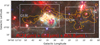 |
Fig. 1 Three-color composite image – MIPS 24 μm (red), IRAC4 8 μm (green), and IRAC3 5.8 μm (blue) – of the field containing G53. Two white rectangular boxes enclose the areas of G53W and G53E. The contours represent13CO (1–0) integrated intensity, with levels of [4, 8, 12, 16, 20]×RMS(= 0.9 K km s–1 ). Two purple stars mark the locations of HII G53.54-0.01 and HII G53.18+0.20. |
Main parameters of the Nanshan telescope.
2 Observations and archival data
2.1 NH3 observations
From February 2024 to April 2024, we conducted observations of NH3 (1,1) and (2,2) lines in G53 using the Xinjiang Astronomical Observatory Nanshan 26-meter radio telescope. We used a dual polarization channel superheterodyne receiver operating in the 22.0–24.2 GHz range, with a frequency centered at 23.708 GHz, to simultaneously observe the NH3 (1,1) and (2,2) lines. At this frequency, the telescope has a primary beam width (full width at half maximum) of ~ 2′ along with a velocity resolution of ~ 0.1 km s–1. The main parameters of the Nanshan 26-meter radio telescope are listed in Table 1.
During the observations, the system temperature were maintained at around 50 K on an antenna temperature  scale The elevation angle of the radio telescope was always above 20°. We used the on-the-fly (OTF) mapping mode, with each OTF map covering an area of 6′ × 6′ and an angular sampling step of 1′. All observations were conducted under clear weather conditions, resulting in a typical root mean square (RMS) noise level of ~25 mK.
2.2 Archivai data
2.2.1 The CO molecular data
The 13CO (1–0) data were obtained from the Boston University-Five College Radio Astronomy Observatory Galactic Ring Survey (GRS) with an angular and spectral resolution of 46″ and 0.21 km s–1, respectively, and a typical RMS sensitivity  . The survey used the SEQUOIA multi pixel array on the Five College Radio Astronomy Observatory 14 m telescope to cover a longitude range of l = 18°–55.7° and a latitude range of |b| < 1°, resulting in a total of 75.4 square degrees (Jackson et al. 2006).
We also used 12CO (3–2) data from the CO High-resolution Survey (COHRS; Park et al. 2023), which has mapped the inner Galactic plane over the range of 9.5° < l < 62.3° and |b| < 0.5° using the HARPS instrument on the James Clerk Maxwell Telescope (JCMT). These data have a spatial resolution of 16.6″ and a velocity resolution of 0.635 km s–1, achieving a mean RMS of ~0.6 K on  .
.
2.2.2 The infrared data
Hi-GAL, an Open Time Key Project of the Herschel Space Observatory made an unbiased photometric survey of the inner Galactic plane by mapping a 2° wide strip in the longitude range |l| < 60° in five wavebands between 70 μm and 500 μm (Molinari et al. 2010b). The Herschel Space Observatory is equipped with three instruments, Photodetector Array Camera and Spectrometer (PACS; Poglitsch et al. 2010), Spectral and Photometric Imaging Receiver (SPIRE; Griffin et al. 2010) and the Heterodyne Instrument for the Far Infrared (HIFI). PACS is responsible for the 70 μm and 160 μm bands, while SPIRE handles the 250, 350, and 500 μm bands. Data from the heterodyne instrument HIFI are not used in the following. Due to the predominantly single-velocity component spectra of the molecular cloud G53 (see below), we were able to utilize the Herschel H2 column density and temperature maps. Notably, only a small region (less than 10% of all pixels) exhibits a second velocity component in 13CO(1–0), located near l=53.35°, b=0.03°. We downloaded the Herschel H2 column density and dust temperature maps from the publicly available website1. These maps were generated for the EU-funded ViaLactea project (Molinari et al. 2010b). To create these maps, the Bayesian algorithm, the point process mapping method (Marsh et al. 2015, 2017) was applied to the Herschel images at 70, 160, 250, 350, and 500 μm.
The Infrared Array Camera (IRAC; Fazio et al. 2004) and Multiband Imaging Photometer (MIPS; Rieke et al. 2004) on board the Spitzer Space Telescope (Werner et al. 2004) provided a mid-infrared survey (3.6, 4.5, 5.8, 8.0 and 24, 70 μm) of the Inner Galaxy. The Spitzer 3.6, 4.5, 5.8, 8.0, and 24 μm data are used in this paper to fit the spectral energy distribution (SED) of young stellar objects (YSOs).
3 Results
In this section, we present the results of the NH3 and CO molecular data as well as infrared continuum maps. Included are also some physical parameters deduced from these measurements.
3.1 NH3 map
We extracted spectral data with a signal-to-noise ratio greater than 2.5 σ and created a velocity-integrated intensity map (Fig. 2, top panel) for NH3(1,1) with an integration range of 20–26 km s–1. We present the NH3 (2,2) spectrum of Region 1 in the inset plot of the top panel. The bottom panels show the NH3(1,1) spectra and fitting lines for the six regions. The detailed fitting method for NH3 is provided in Appendix A. The fitted parameter results are annotated at the top-left corner of each plot. Figures A.1a and A.1b depict maps of the center velocity and line width (of the central group of hyperfine components) obtained through fitting NH3(1,1), respectively.
3.2 CO gas morphology
We used GAUSSPY+2, a fully automated Gaussian decomposition package for emission line spectra (Lindner et al. 2015; Riener et al. 2019), to perform multicomponent Gaussian fitting on the13 CO (1–0) data of the G53 region and extracted the spectral data with center velocities between 20 and 26 km s–1 .In this paper, all velocities are with respect to the local standard of rest (LSR). We then mapped the integrated intensity, center velocity, and line width obtained from the fitting (see Fig. 4). Note that if a pixel has multiple velocity components within the range of 20–26 km s–1, we took their integrated intensity-weighted average for both the central velocity and the line width. In the 13CO (1–0) fitting process, we neglected the effects of self-absorption, as 13CO (1–0) is optically thin in the G53 region. Furthermore, a detailed analysis of the optical depth of 13CO (1–0) in G53 is presented in Appendix B. For the 12CO (3–2), we used moment maps in Fig. 4, rather than GAUSSPY+ fitting parameters. Because the 12CO (3–2) exhibits strong self-absorption in some dense regions (as shown in Fig. 9).
The 13CO (1–0) line traces the morphology of the entire G53 region. Figure 4 shows all the kinematic information of G53. Between 21 and 25 km s–1, G53 exhibits an elongated cloud structure. In Figs. Ea (the Berschel H2 column density) and Eb (the H2 column density derived from Fig. 4a), it is evident that material accumulates at both ends of G53, forming two dense regions, G53E and G53W (indicated by the white rectangles in Fig. 1). In Fig. 4c, it can be seen that the line width of G53W is slightly larger than that of G53E, which may indicate the presence of stronger turbulence in G53W. Figure 4b indicates that the G53W region exhibits a velocity gradients. For a detailed discussion, see Sect. 4.1.3.
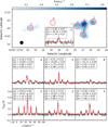 |
Fig. 2 Map and spectral lines of the NH3 (1,1). Top panel: velocity-integrated intensity map of the NH3 (1,1) main group of hyperfine components with an integration range of 20–26 km s–1. Six red circles mark the six main regions; each circle has a diameter of 3.33′. The inset shows the NH3(2,2) spectrum of Region 1. The p1, p2, and p3 represent the peak intensity in K, the line center velocity in km s–1, and the line width in km s–1, respectively. The black circle in the lower-left corner represents the beam size. Bottom panel: Ammonia (1,1) spectra for the six regions. The p2, p3, and p4 represent the line center velocity (Vlsr) in km s–1, the line width (ΔV) in km s–1, and the main group peak optical depth (τmain), respectively. p1 = A0 × τmain, where A0 is an arbitrary amplitude in units of K. Although A0 is an arbitrary amplitude, when τmain ≪ 1, A0 corresponds to the main group peak intensity. |
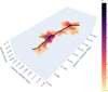 |
Fig. 3 13CO (1–0) PPV cube in G53 (magma) and the filament spine (black) and branches (green) identified from the cube using CRISPY. |
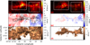 |
Fig. 4 Panels a–c: integrated intensity, center velocity, and line width of the 13CO (1–0) spectral data fitted using GAUSSPY+, respectively. The contours in panel a represent the NH3(1,1) main line integrated intensity, with contour levels of [3, 6, 9]×RMS(=0.06 K km s–1). The contours in panels b) and c represent the 13CO (1–0) integrated intensity, with contour levels of [4, 8, 12, 16, 20]×RMS(=0.9 K km s–1). Panels d–f: moment 0, moment 1, and moment 2 maps of the 12CO (3–2) transition, rather than the parameters from GAUSSPY+ fitting due to its self-absorption. The white rectangles in panels a and d are same as that in Fig. 1. |
3.3 Properties of the filament
Ragan et al. (2014) recognized the G53 molecular cloud as a coherent velocity filamentary structure. To conduct a detailed investigation of its filamentary properties, we utilized CRISPY3, a Python package designed to identify filament spines in 3D images (e.g., position–position–velocity cubes; Chen et al. 2014, 2020), to identify the 13CO (1–0) filament spine within G53 (see Fig. 3). The core of CRISPY relies on the subspace constrained mean shift (SCMS) algorithm. The mathematical framework behind SCMS was generalized by Chen et al. (2014) to operate on weighted, particle-like data in addition to their unweighted counterparts, which enables SCMS to run on gridded, multidimensional images. We applied an over-mask parameter to filter out pixels with intensities below 0.2 K in the 13CO (1–0) position-position-velocity (PPV) space, and set the minimum intensity threshold to 0.7 K. Additionally, to focus on the properties of the filament spine, we removed branches containing fewer than 2pc (which is width of the filament G53). The sky-projected length of the filament spine calculated using pruning method (this method is based on 2D version FilFinder4) in CRISPY is 30 pc. Based on the sky-projected spine, We used RadFil, a publicly available Python package5 to build and fit a radial profile (Zucker & Chen 2018), to fit the width of the spine with a Plummer function (see Appendix C), resulting in a full width at half maximum (FWHM) of 2.0 ± 0.4 pc (~4′). Its aspect ratio can be calculated as A = 15 ± 0.3.
We collected young stellar objects (YSOs; Kim et al. 2015) and dust cores from The ATLASGAL survey (Csengeri et al. 2014) in G53, respectively. Based on the IR spectral index defined as  , these YSO candidates are classified by Kim et al. (2015) as Class I (0.3 ≤ α, the youngest evolutionary class whose SED is rising toward the middle-IR, which indicates the presence of a dusty envelope infalling onto a central protostar), Flat spectrum (–0.3 ≤ α < 0.3, objects whose evolutionary status is likely between Class I and II), Class II (–1.6 ≤ α < –0.3, pre-main-sequence stars with warm optically thick dusty disks) and Class III (–2.56 ≤ α < –1.6, objects whose SED is mostly photospheric emission in the near-IR but which show some excess emission at longer wavelengths). These different types of YSOs are marked with different colors of star markers (red: Class I, yellow: Flat spectrum, green: Class II, blue: Class III).
The dense clumps on the filament G53 spine were identified using the astrodendro6 on the Herschel H2 column density map. In relation to Fig. 5, the dense material of regions 1 and 2 were identified as clumps C2 and C4, while the dense material of regions 6 and 7 were identified as clumps C3 and C1, respectively. Their shapes and positions on the sky plane are marked in Fig. D.1, and their physical parameters are listed in Table D.1. Detailed identification procedures can be found in Appendix D.
To better understand the kinematic information of the filament, we plotted the variation curves of different physical quantities along the spine of the filament. Figure 6 presents these results. Figures 6c and 6d show the distribution of the Herschel H2 dust temperature and column density. The green line in Fig. 6d represents the H2 column density derived from 13CO (1–0) (see Appendix E). It is evident that the material density in regions C1 and C3 of G53E, as well as in C2 and C4 of G53W, is significantly higher than in other areas. This may be due to the filament G53 undergoing EDC, where dense clumps form at the ends of the filament and converge toward the center, sweeping up mass as they move (Clarke & Whitworth 2015). Figures 6e and 6f show the distribution of center velocities and line widths fitted by GAUSSPY+ for 13CO (1–0). Two solid red line segments in Fig. 6e represent the velocity gradients along the filament spine at the locations of clumps C2 and C4, which are –0.17 and –0.74 km s–1 pc–1, respectively. The vertical dashed red lines represent the four clumps identified using the astrodendro on the Herschel H2 column density map. Figure 6g shows the surface density of YSOs at different stages along the filament spine. G53W C2 and G53E C1, C3 exhibit higher numbers of Class I, Flat spectrum, and Class II objects.
To assess the stability of the filament G53, we calculated the observed line mass (the ratio of the filament mass and length) and the virial line mass per parsec lengths of the filament. For the calculation of the virial line mass, we used the method applied by Dewangan et al. (2019) and He et al. (2023a). Using the 13CO data, the calculated virial line mass of the filament G53 is 264 ± 28 M⊙ pc–1, and the virial line mass derived from NH3 is 259 ± 24 M⊙ pc–1. For a detailed explanation of the calculation methods, please refer to Appendix F. For the calculation of the mass of the filament spine, we simply summed the Herschel H2 column density, and the result is 7966 ± 3168 M⊙. We further determined the observed line mass that is 265 ± 105 M⊙ pc–1. The virial line mass and the observed line mass are of the same order of magnitude, which may suggest that the entire filament is in virial equilibrium.
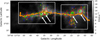 |
Fig. 5 Sky-projected filament spine. The background is the 13CO velocity-integrated intensity map. The orange corresponds to the sky-projected spine extracted by CRISPY. The lime ellipses represent dust cores from the ATLASGAL survey. The star markers in different colors represent YSOs at different stages: Class I (red), flat spectrum (yellow), Class II (green), and Class III (blue). The region marked with a red circle is the area of interest to us, where regions 1, 2, and 6 are labeled the same as in the top panel of Fig. 2, and region 7 is an additional region based on the top panel of Fig. 2. Region 7 shows a signal in CO and the Herschel H2 column density map, but no signal in NH3. White arrows indicate the positions of the end clumps in G53W and G53E. In G53W, the end clumps are located in regions 1 and 2, while in G53E, the end clumps are found in regions 6 and 7, as clearly depicted in the Herschel H2 column density map (shown in Figs. 7 and D.1). |
3.4 Gravitational field
Based on the Herschel H2 column densities, we calculated the 2D-projected gravitational potential field ϕ(x, y) of the filament G53 using phi_2d code7, which solves the 2D poisson equation in phase space based on the 2D column density distribution. This calculation method has been previously discussed in detail by He et al. (2023b) and Zhou et al. (2024). Following Appendix A in Zhou et al. (2024), We calculated the two eigenvalues (λmin and λmax, as shown in Fig. 7) of the tidal tensor using the following equation,

where T is the tidal tensor and its element is Tij = ∂i∂jϕ, and λ and a represent the eigenvalues and eigenvectors of the tidal tensor, respectively. The two eigenvalues control the motions of the gas along two orthogonal directions. If the eigenvalue is less than zero, the gas is expanding; if the eigenvalue is greater than zero, the gas is contracting (Li 2024). Figures 7a and 7b present the maps of λmax and λmin, Fig. 7c shows the direction of the gravitational field in G53, and Fig. 7d illustrates the directions of the two eigenvectors. Figures 6a and 6b plot the distribution of the gravitational potential and λmin along the filament spine, respectively. The gravitational potential wells are primarily located in the G53E and G53W regions.
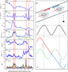 |
Fig. 6 Distribution of different physical parameters along the filament spine (see the orange line in Fig. 5). These physical quantities are the averaged values within a beam (46″) at the blue points in the top-left panel of Fig. C.1. Panels a and b: distribution of the gravitational potential and λmin (see Sect. 7) along the spine of the filament, respectively. Panels c and d: Herschel dust temperature and H2 column density (blue) and the H2 column density derived from 13CO (1–0) (green). Panels e and f: distributions of the center velocity and line width obtained by fitting 13CO (1–0). Their errors arise from the Gaussian fitting process. Panel g: YSO area density: total YSOs (black), Class I (red), flat spectrum (orange), Class II (green), and Class III (blue). The vertical dashed red lines mark the positions of clumps. Panel h: schematic diagram of the core formation model, which is explained in Sect. 4.1.3. Panel h: density profile along the projected filament (ρ) and velocity profile along the projected filament (VLSR). The two sets of velocity profiles in the bottom panel indicate two different scenarios. The dashed green line represents the velocity profile generated under the condition that the two clumps’ centroids are at rest relative to each other while accreting material along the filament. The solid line (composed of two segments, in red and blue) represents the velocity profile generated under the condition that the two clumps are moving toward each other while also accreting material along the filament. Red and blue curves represent redshift and blueshift clumps, respectively. |
3.5 ATLASGAL dust cores
We selected the dust cores located in the molecular cloud G53 from Table 2 of Csengeri et al. (2014) and marked them with lime ellipses in Fig. 5. To understand the gravitational stability of the dust cores in G53, we calculated the observed mass and virial ratio of these cores. The calculation method of observed mass is the same as that in Sect. 3.3. The calculation results are shown in Table G.1, column 7. Following Williams et al. (2018), we used a uniform sphere to assess the virial ratio,
 (1)
(1)
where aeff is the total velocity dispersion considering both thermal and nonthermal contributions from all molecules. We used the velocity dispersion of 13CO (1–0) as an approximation for aeff. R is the effective radius of the analyzed dust cores. M is the observed mass. The calculation results are shown in Table G.1 (Col. 8). The average virial parameter of the dust cores in the G53W region is 8.88, which is higher than the average value of 3.26 in the G53E region.
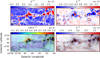 |
Fig. 7 Panels a and b: maps of the eigenvalues of the tidal tensor λmax and λmin (refer to Sect. 3.4) toward G53. The solid black ellipses represent C1, C3, C2, and C4 from left to right. The dashed black circles represent regions 4 and 3 from left to right. Panel c: Herschel H2 column density. Thee color and direction of the arrows indicate the magnitude and direction of the gravitational field. Panel d: same as panel c but with two opposing arrows in one direction indicating that the gas in this pixel is collapsing along the corresponding directions, while two arrows pointing away from each other indicate the gas in this pixel is expanding along the corresponding directions. |
4 Discussion
4.1 EDC in the molecular cloud G53
4.1.1 Evidence of an end-dominated collapse in G53
The numerical simulations of Clarke & Whitworth (2015) show that a filament with an aspect ratio A ≳ 5 and uniform density will undergo an EDC. In Sect. 3.3 we calculated the aspect ratio of the filament G53 as A ~ 15 > 5, which satisfies the conditions for an EDC. As shown in Fig. 4a, the dense gas clumps are concentrated at the two ends of the filament G53, indicating an onset of an EDC. Additionally, Fig. 6 also indicates signs of an EDC. For example, panel g shows the formation of two stellar clusters at the ends of the filament, G53E and G53W, and panel d shows a significant increase in H2 column density for G53e and G53W.
Signs of an EDC can also be observed from the kinematics of the gas, as shown in Figs. 4b and 6e. There is a significant velocity difference between C4 in the G53W region and C1 and C3 in the G53E region, which resembles the velocity field produced by the numerical simulation of EDCs (see Sect. 4.2). However, C2 in the G53W region shares a similar velocity with G53E, which will be discussed in Sect. 4.1.3.
Both G53W and G53E lie near the edges of the HII regions G53.54-0.01 and G53.18+0.20 (marked by purple stars in Fig. 1). We therefore need to rule out compression from these HII regions as the driver of collapse in G53W and G53E (e.g., through the “collect and collapse” process; Liu et al. 2017). For HII G53.18+0.20, located north of G53W, it belongs to a different velocity component than G53 (as reported by Kim et al. 2015). The HII region G53.18+0.20 is located at 9.7 kpc according to the Red MSX Source survey (Lumsden et al. 2013), which places it 8 kpc more distant than G53. This substantial separation in distance demonstrates that there is no physical connection between HII G53.18+0.20 and the G53. As for HII G53.54-0.01, adjacent to G53E, we find no kinematic evidence of HII feedback. Instead, HII G53.54-0.01 is likely part of G53E, where ionization has eroded the central gas, leaving only the periphery observed today.
4.1.2 Collapse timescale for the filament G53
Following the method of Yuan et al. (2020) for calculating collapse timescales of filaments, we used
 (2)
(2)
where ΔL = Lbefore – Lafter, and  . From the integrated intensity map of 13CO (1–0) (as shown in Fig. 4a), it is evident that there is a long gas tail in the eastern region of G53E. We believe this may be due to the original filament undergoing an EDC, causing the end clumps to move inward and leaving residual gas in their original positions. Therefore, for the filament G53 we can estimate the length of the filament prior to the EDC, Lbefore ≃ 30 pc, based on the extent of the filament gas, and estimate the current length of the filament, Lafter ≃ 14 pc, using the distance between the end clumps. We assumed that the average length of the filament during the EDC process is given by
  , and the filament width d ≃ 2 pc. The collapse time of the filament G53 is about 5.53 Myr. Additionally, we used the formula from Clarke & Whitworth (2015), tco1 ~ (0.49 + 0.26A)(Gρ)–1/2, to calculate the collapse timescale of the filament G53, resulting in 7.04 Myr. In this calculation, we assumed a cylindric geometry to calculate the volume density before collapse, which is ρ = Mf /(Lbefore × π × (d/2)2) = 5.73 × 10⁻²¹ g cm–3. Note that the time calculated using the method from Yuan et al. (2020) represents the time taken for the filament to collapse to its current state, while the time calculated using the method from Clarke & Whitworth (2015) refers to the moment when the two converging end-clumps merge. The latter exceeds the former by approximately ~1.3 Myr, indicating that G53 still requires nearly 1.3 Myr for the two converging end-clumps to merge.
4.1.3 Velocity distribution along the filament G53
Figure 6e shows the velocity profile along the filament spine, indicating a ~3 km s–1 velocity variation for the filament G53. The largest velocity gradient occurs between C2 and C4 in G53W. There are three possible explanations for the velocity gradient along the filament: (1) rotation, (2) local collision, and (3) gravitational accretion along the filament during core formation. The local velocity difference between C2 and C4 is unlikely to be caused by rotation, as such a scenario could tear apart the filament (Peretto et al. 2014; He et al. 2023a). Therefore, we interpreted this velocity gradient in the context of core formation and core collision. The velocity profile and column density profile at the positions of C2 and C4 may be explained by the core formation model from Hacar & Tafalla (2011). In Fig. 6h, we present the velocity distribution of VLSR produced by two clumps that are either at rest relative to each other or moving toward each other under the core formation model. The dashed green line indicates the velocity profile when the two clumps are at rest; if the two clumps move toward each other, it will result in redshift and blueshift at the locations of the two clumps, producing the velocity profile depicted by the solid line (composed of two segments: red and blue curves). This is similar to the velocity profile corresponding to C2 and C4 in Fig. 6e. This further indicates that C2 and C4 in the G53W region are converging based on the significant velocity difference observed at C2 and C4 in Fig. 6e. This scenario is similar to the EDC model from our numerical simulations discussed in Sect. 4.2. Assuming that the velocity of the clumps remains unchanged during their motion and that the clumps move at an angle of 45° to the line of sight, we calculated the time required for C4 and C2 to collide, which is at the order of 1 Myr. On a large scale, G53W and G53E are moving toward each other, with a velocity difference between C1 (or C3) and C4 of approximately 3 km s–1. Figure 8 presents a schematic diagram of the motion in G53.
 |
Fig. 8 Schematic cartoon of the kinematics of G53? Colored arrows indicate the movement directions of the molecular cloud and clumps, and the dashed black line represents the line-of-sight direction. |
4.1.4 Infall motion in clump C4
We also find signs of infall from 12CO (3–2) and C18O (1–0) spectra in clump C4. The optically thick 12CO(3–2) spectral line shows a red-blue asymmetric profile, with the blue side higher than the red side. In contrast, the optically thin C18O(1–0) exhibits a single peak, located between the red and blue ends of the 12CO (3–2) line, as shown in Fig. 9. Following Yang et al. (2020), we can further quantify the asymmetry of the12CO (3–2) line determining δV in the following way:
 (3)
(3)
where Vthick and Vthin represent the peak velocities of the optically thick and thin lines, respectively, and ΔVthin is the FWHM of the optically thin line. We used C18O (1–0) as the optically thin line and calculated the asymmetry of the 12CO(3–2) spectrum to be ~–0.94. Following the criteria of Mardones et al. (1997), where sources with δV < –0.25 are considered to have significant blue profiles, sources with δV > 0.25 are considered to have significant red profiles, and sources with –0.25 < δV < 0.25 exhibit asymmetry profiles, clump C4 can be identified as an infall source. We calculated the infall velocity of clump C4 using the following formula (Myers et al. 1996):
 (4)
(4)
where Vred and Vb1ue are the velocities of the red and blue peaks of the optically thick line, while Tred and Tblue are the corresponding peak intensities. Tdip is the intensity of the self-absorption dip between the two peaks. Note that this formula assumes that the infall velocity is Vinf ≪ ΔVthin(2 ln τ)1/2. We calculated the infall velocity of clump C4 to be Vinf ~ 0.37 km s–1. We further calculated its mass infall rate, Ṁinf = 4πR2Vinfn ~ 372 M⊙ Myr–1, where n=Mc1ump/(4/3πR3) is the average clump volume density, and R (~0.3 pc) is the effective radius of the clump extracted from the astrodendro. This is consistent with the mass infall rate (102–104 M⊙ Myr–1; He et al. 2015; Yang et al. 2020) in massive star formation regions.
4.2 Simulation of EDCs
Burkert & Hartmann (2004) presented 2D simulations of finite, self-gravitating gaseous sheets under an elliptical outer boundary. The results showed that the sheets eventually collapsed into a filamentary structure, with material accumulating at the ends of the filament. Later, Clarke & Whitworth (2015) specifically studied the collapse time of filaments using smoothed particle hydro-dynamic simulations of cold, uniform-density, self-gravitating filaments. They provided an estimate for the time required for the two end clumps to merge. To gain a clearer understanding of how a finite, truncated filament undergoes EDC in a turbulent medium, the nonviscous compressible hydrodynamic numerical simulation of an EDC was presented using the Athena++ code8 (Stone et al. 2020) with adaptive mesh refinement and the full multi-grid mode of the multi-grid self-gravity solver. We used a 3D isothermal cylinder with the thermal sound velocity cs = 0.2 km s–1 as the initial condition for the numerical simulation. The radial density distribution of the cylinder is (Ostriker 1964; André et al. 2014)
![Mathematical equation: $\rho \left( r \right) = {{{\rho _c}} \over {{{\left[ {1 + {{\left( {r/{R_{{\rm{flat}}}}} \right)}^2}} \right]}^{p/2}}}},$](/articles/aa/full_html/2025/09/aa53390-24/aa53390-24-eq12.png) (5)
(5)
where ρc = 1 × 10–22 g cm–3, Rflat = 2 pc, and p = 4 (this set of parameters allows thermal pressure to balance gravitational forces). The entire simulation was conducted on a 3D Cartesian grid with NX × NY × NZ = 256 × 256 × 256, with the physical range of X, Y, and Z axes from –10 to 10 pc. At evolution time t = 0 Myr, the axis of the 16 pc cylinder reunites with the Z axis. To reproduce a more realistic molecular cloud environment, we injected a velocity perturbation with a velocity power spectrum ∝ k–2 (where k is wave number; Gong & Ostriker 2011) into the grid at the beginning of the evolution.
We ran the simulation for 14 Myr, by which time two dense clumps had formed at the ends of the filament. We extracted three 2D snapshots at Y = 0 pc, as shown in Fig. 10, corresponding to evolution times of 2.17 (left panel), 6.51 (middle panel), and 10.22 (right panel) Myr. The background represents the velocity field υz in the Z direction, and the contours indicate the density distribution. At t = 6.51 Myr (middle panel), signs of an EDC begin to appear. There is a noticeable velocity gradient in the regions of the dense clumps at both ends, indicating that the two dense clumps are moving toward each other. This is very similar to the velocity field observed in Fig. 4b.
In our numerical simulations, it is observed that under the initial turbulent perturbations, the filament begins to fragment into several approximately equidistant clumps. Subsequently, due to edge effects, the clumps at the ends of the filament merge with each other. This phenomenon is similar to the observed motion of C4 and C2 toward each other in the G53W region.
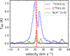 |
Fig. 9 Averaged spectra of different molecules in clump C4, calculated from the regions indicated by the red elliptical area in Fig. D.1. This includes in blue the 12CO (3–2), in red the C18O (1–0), and in green the N2H+ (1–0) transitions. The C18O (1–0) and N2H+ (1–0) data were obtained from Zhang et al. (2017) using observations from the IRAM 30 m telescope. Note that the condition for generating a blue-red asymmetry spectrum is that the cloud must exhibit a central condensation of material. We assumed that clump C4 satisfies this condition. |
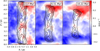 |
Fig. 10 2D snapshots (Y = 0 pc) at evolution time t = 2.17 (left panel), 6.51 (middle panel), and 10.22 (right panel) Myr. The Z direction is along the axis of the cylinder (note that the positive direction of the Z axis is downward), while X and Y are the two orthogonal directions perpendicular to the Z axis. The background is the velocity along Z axis (υz). The contours mark the distribution of the filament cloud density, with levels of 0.74, 0.99, 1.40, and 1.87 ×10⁻²² g cm–3. |
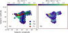 |
Fig. 11 Panel a: NH3 (1,1) line width obtained using the fitting method described in Appendix A. The blue, green, and red scatter markers represent Fe, Fw, and Fs, respectively, which correspond to the three branches connecting the hub center. Panel b: magnitude of the line-of-sight velocity gradient. The arrows indicate the direction of the velocity gradient. The solid red ellipses represent C2 and C4, and the dashed red circles represent regions 4 and 3. |
4.3 Kinematics inside the hub-filament system
HFSs are widespread sites of massive star formation within the interstellar medium (ISM). Understanding the origin of HFSs is crucial in explaining the process from molecular cloud formation leading to the development of dense cores. In the G53W region, the velocity-integrated intensity map of NH3 (1,1) (see Fig. 2) reveals a HFS centered on C2.
Figure 11 illustrates the HFS observed in G53W through the NH3 (1,1) velocity-integrated intensity map. The different colored circular markers represent various filament (actually, Fe and Fw are the segments of the filament spine, while Fs is a branch connected to the spine) connected to the hub center. We used the NH3 (1–0) molecular lines to analyze the kinematics of the G53W HFS. Figure 12a shows the distribution of the NH3(1,1) centroid velocity along Fe, Fw, and Fs. A significant velocity gradient can be observed along each filament starting at their common origin. In Sect. 4.1.3 we have discussed the velocity difference along Fw, interpreting it as the converging motion of clumps C2 and C4. Similarly, the velocity differences along Fe and Fs are also interpreted as the result of material in Regions 3 and 4 (top panel of Fig. 2) moving toward the central hub, consistent with the behavior observed at the ends of molecular clouds in our numerical simulations of the EDC. Another notable kinematic feature of G53W is the significant correlation between the velocity gradient and the NH3(1,1) line width (their spearman correlation coefficient is 0.74 and p-value << 0.05). Figures 11a and 11b display the line width and line-of-sight velocity gradient maps of NH3 (1,1), respectively, both showing higher values around the hub center, C2. Figures 12b and 12c illustrate the distribution of velocity gradient and line width along the filament branches, demonstrating a clear consistency between the two. Additionally, we performed a spearman statistical analysis on the line width and velocity gradient for all pixels in G53W, with results presented right panel in Fig. 13. To further analyze whether this line width distribution is caused by gravitational or tidal effects on larger scales, we also performed a spearman analysis between the line width and the gravitational potential as well as λmax – λmin (which can characterize the degree of deformation of the gas due to tidal forces), as shown in the left and middle panels of Fig. 13. Based on their relatively weak correlation coefficients (–0.09 and 0.13), we cannot conclude that this line width distribution is caused by gravitational or tidal effects. We guess that this phenomenon could be due to the relative motion between clumps, which enhances turbulence in the compressed gas layers between them, resulting in broader line widths. However, due to our limited resolution, the effects of protostellar feedback, infall motions, and beam smearing cannot be ruled out. Higher-resolution observations may be needed in the future to study molecular kinematics on smaller scales.
To understand the star formation in the HFS regions G53E and G53W, we utilized data from Kim et al. (2015) (Table 2), which lists the YSOs located in the G53 molecular cloud, including their magnitudes from the Two Micron All Sky Survey (2MASS) in the J, H, and Ks bands, and from the IRAC bands of 3.6, 4.5, 5.8, and 8.0 μm, as well as the MIPS band at 24 μm. We obtained the physical parameters of these YSOs by fitting their SED using the method9 described by Robitaille et al. (2006). These physical parameters include the mass and age of the YSOs. We calculated the total mass M★ total and average age t★ of the YSOs located in G53W and G53E. Using these parameters, we further determined the star formation efficiency (SFE) of G53W and G53E. SFE is defined as the ratio of the total mass of all YSOs to the mass of the molecular cloud, given by  . The results are shown in Table 2. It can be seen that G53W and G53E have similar evolutionary timescales and SFE. In addition, we also calculated SFE and star formation rate
  for the seven regions shown in Fig. 2 and 5, as listed in Table 2. It can be seen that Region 1 has a relatively high SFE and SFR, which may be related to its position at the hub center of G53W. This location allows it to receive material flows from three filament branches, nurturing the formation of massive stars within it. The mass accretion flow of Region 1, as calculated in Sect. 4.1.3, is fully sufficient to sustain the SFR in Region 1.
Information of YSOs in G53.
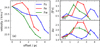 |
Fig. 12 Distributions of the line-of-sight velocity (a), velocity gradient (b), and line width (c) along the Fe, Fw, and Fs given in Fig. 11a, starting at their common origin. These physical quantities are extracted from the central pixel values of the colored circles in Fig. 11a. |
5 Conclusions
Combining numerical simulations, archival data, and our own observations of NH3, we conducted an investigation on the kinematics and star formation activity of the molecular cloud G53. The results are summarized as follows:
We mapped the NH3 (1,1) emission in G53 and found a relatively strong signal in the G53W region, where the NH3 morphology displays a HFS. However, in the G53E region, the NH3 (1,1) signal is very weak and the mapping range is particularly small. The NH3 (2,2) line was only detected in Clump C2 of G53W;
We used CRISPY to identify the filamentary structures in the PPV space of 13CO(1–0) for G53. The results show that material accumulates at both ends of the filament, forming a HFS at these ends. We also calculated the gravitational potential, which is in accordance with an accretion of material toward the ends. Most of the YSOs in the G53 region are concentrated at the ends of the filament (G53W and G53E), which may indicate that the EDC (where the ends of a finite filamentary structure collapse more rapidly than the central regions) of the filament has triggered star formation at both ends;
We analyzed the position-velocity diagram along the spine of the filament and found velocity gradients at C2 and C4, which may indicate material flow along the filament. Additionally, we found signs of infall into Clump C4 (red-blue asymmetry in 12CO (3–2)). The velocity difference between C2 and C4 suggests that the two clumps are moving toward each other;
We conducted hydrodynamic simulations of the EDC in a turbulent filament. The simulation results show that a critically stable isothermal cylinder, under turbulent perturbations, first fragments into several equally spaced clumps, which then merge toward the ends. These clumps eventually merge into two end clumps. This is consistent with our initial guess that C2 and C4 in G53W are moving toward each other;
Using NH3(1,1), we found a significant correlation between the line width and the velocity gradient in the G53W region. This line width distribution may indicate large-scale turbulence caused by the accumulation motion of the material;
We investigated the SFE in the G53 region by fitting the SEDs of YSOs. It was found that the SFE at the hub center, C2, in G53W is relatively high, which may be due to its location at the hub center, receiving sufficient material inflow to sustain star formation.
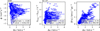 |
Fig. 13 Correlation between the line width and gravitational potential (left panel), λmax – λmin (middle panel), and velocity gradient (right panel) in the G53W region. λmax – λmin can characterize the degree of deformation of the gas due to tidal forces. The calculation of λmax and λmin is provided in Sect. 7. The Spearman correlation coefficient and p-value are labeled in the bottom-right corner of each panel. Note that each data point corresponds to a single pixel. Native pixels are not independent, due to beam convolution. |
Acknowledgements
We thank the referee for providing constructive comments that substantially improved the quality of the paper. This work was main funded by National Key R&D Program of China under grant Nos. (2023YFA1608002 and 2022YFA1603103) and Tianshan Talent Training Program 2024TSYCTD0013. It was also partially funded by the Regional Collaborative Innovation Project of Xinjiang Uyghur Autonomous Region grant 2022E0105, the NSFC under grants 12173075, 11973076, 12103082 and 12403033, the Natural Science Foundation of Xinjiang Uygur Autonomous Region under grant 2022D01E06, the CAS Light of West China Program 2021-XBQNXZ-028 and XBZG-ZDSYS-202212, the Xinjiang Key Laboratory of Radio Astrophysics under grant 2022D04033, The Tianshan Talent Program of Xinjiang Uygur Autonomous Region under Grant No.2022TSYCLJ0005, the Youth Innovation Promotion Association CAS, the Tianchi Talent Project of Xinjiang Uyghur Autonomous Region. This work is based on observations made with the Nanshan 26m radio telescope, which is operated by the Key Laboratory of Radio Astronomy, Chinese Academy of Sciences. In addition, this publication makes use of molecular line data from the Boston University-FCRAO Galactic Ring Survey (GRS). The GRS is a joint project of Boston University and Five College Radio Astronomy Observatory, funded by the National Science Foundation under grants AST-9800334, AST-0098562, & AST-0100793. C. Henkel has been funded by Chinese Academy of Sciences President’s International Fellowship Initiative grant No. 2025PVA0048. A.M. Sobolev has been funded by Chinese Academy of Sciences President’s International Fellowship Initiative grant No. 2024VMA0002 and by the Ministry of Science and Higher Education of the Russian Federation by an agreement FEUZ-2023-0019.
Appendix A Fitting NH3
Assuming that the optical depths of the five groups of hyperfine components of NH3 (1,1) are Gaussian functions, the total optical depth is the sum of these five components:
![Mathematical equation: $\tau \left( \upsilon \right) = {p_4}\mathop \sum \limits_{i = 1}^N {r_i}\exp \left[ { - 4\ln 2{{\left( {{{\upsilon - {\upsilon _i} - {p_2}} \over {{p_3}}}} \right)}^2}} \right].$](/articles/aa/full_html/2025/09/aa53390-24/aa53390-24-eq15.png) (A.1)
(A.1)
According to radiative transfer theory, the main beam brightness temperature TMB(υ) can be given by the following equation:
 (A.2)
(A.2)
where υi and ri represent the velocity offset and the intensity relative to the main component. p2, p3, and p4 represent the line center velocity (Vlsr), line width (ΔV), and main group optical depth (τmain), respectively. p1 = A0 × τmain (A0 is an arbitrary amplitude that is constrained by the measured TMB value). We used Eq. A.2 to fit NH3 (1,1).
For NH3 (2,2), we performed a simple Gaussian fit, where p1, p2, and p3 represent the peak intensity, line center velocity, and line width, respectively.
 |
Fig. A.1 Maps of the center velocity (a) and line width (of the main group of hyperfine components; b) obtained through fitting NH3(1,1). The contours represent the velocity-integrated intensity of NH3(1,1), with levels of 0.60, 0.80, 1.13, and 1.50 K km s–1. |
Appendix B Optical depth calculation of the 13CO (1-0)
In this section we calculate the optical depth of 13CO (1-0) in the G53 region using Eq. B.2, assuming Tex = 20 K. Figure B.1 presents the optical depth distribution of all pixels in the G53 region, showing that most pixels have an optical depth of less than 0.1.
 (B.1)
(B.1)
 (B.2)
(B.2)
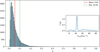 |
Fig. B.1 Histogram of the 13CO (1-0) optical depth in G53. The inset shows the averaged 13CO (1-0) spectral line for the entire G53 region (mapping region of Fig. 5). |
Appendix C Fitting of the spine width
Based on the sky-projected spine, We used RadFil, a publicly available Python package to build and fit a radial profile (Zucker & Chen 2018), to fit the width of the filament G53 with a Plummer function:
![Mathematical equation: ${\rm{N}}\left( {\rm{r}} \right) = {{{{\rm{N}}_0}} \over {{{\left[ {1 + {{\left( {{{\rm{r}} \over {{{\rm{R}}_{{\rm{fat}}}}}}} \right)}^2}} \right]}^{{{p - 1} \over 2}}}}},$](/articles/aa/full_html/2025/09/aa53390-24/aa53390-24-eq19.png) (C.1)
(C.1)
where N0 is the amplitude, p is the power index, and Rfat is the inner flattening radius. Figure C shows the fitting process and result. We used the following formula (Hacar et al. 2023) to calculate the FWHM of the filament:
 (C.2)
(C.2)
resulting in an FWHM of 2.0 pc.
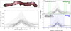 |
Fig. C.1 Top left: Underlying column density of the filament within the spine mask (background grayscale). The thick red line is the smoothed spine of the filament. The perpendicular red cuts are taken tangent to the smoothed spine. The peak column densities along the cut are marked via the blue scatter points. Bottom left: Column density profile along every cut. Right: Background fitting (top) and plummer fitting (bottom) result. |
Appendix D Clump identification
We masked the main region of the filament G53 from the Herschel H2 column density map and used astrodendro to identify clumps in the masked data. The minimum value of H2 column density for clumps identification was set to 8 × 1021 cm–2, which is considered as the threshold for star formation (André et al. 2010, 2014). The other parameters of the astrodendro are set as min_delta = 1 × 1017 cm–2 and min_npix = 30. We adopted equivalent ellipses as the shape of the clumps, and the identification results are shown in Fig. D.1 and Table D.1.
Clumps in the filament G53 spine.
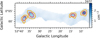 |
Fig. D.1 Herschel H2 column density map (background). The orange contours indicate the column density threshold of 8 × 1021 cm–2. The red ellipses represent the equivalent ellipses of the identified clumps. |
Appendix E The column density from the 13CO versus the Herschel column density
Following Xu & Ju (2014), we calculated the column density of 13CO using the following equation:
 (E.1)
(E.1)
where where the Herschel dust temperature is used as an approximation for the excitation temperature Tex. Then we used the relation  (Simon et al. 2001) to estimate the H2 column density (see Fig. E.1b). To compare with the Herschel column density, we convolved the Herschel column density data to a resolution of 46″ (see Fig. E.1a).
As seen in Fig. E.1a and Fig. E.1b, the Herschel dust and 13CO exhibit similar morphological structures, suggesting that they trace the same molecular cloud. In Fig. E.1c, the blue and orange points represent scatter plots of the column density from 13CO and the Herschel column density in G53E and G53W, respectively. This may indicate a potential difference in the  ratio between G53W and G53E.
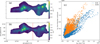 |
Fig. E.1 Panel (a): Herschel column density map. Panel (b): Hydrogen molecule column density derived from 13CO (1-0). The dashed red line represents the boundary between G53W and G53E. Panel (c): Column density derived from the 13CO vs. The Herschel column density. |
Appendix F Calculating the virial line mass of the filament
Following Dewangan et al. (2019) and He et al. (2023a), Mline,vir was calculated as
![Mathematical equation: ${M_{{\rm{line,vir}}}} = \left[ {1 + {{\left( {{{{\sigma _{{\rm{NT}}}}} \over {{c_{\rm{s}}}}}} \right)}^2}} \right] \times \left[ {16{M_ \odot }p{c^{ - 1}} \times \left( {{{{T_{{\rm{kin}}}}} \over {10K}}} \right)} \right],$](/articles/aa/full_html/2025/09/aa53390-24/aa53390-24-eq24.png) (F.1)
(F.1)
where  is the sound speed (μ = 2.37). The nonthermal velocity dispersion is defined as
 (F.2)
(F.2)
where kB is the Boltzmann constant, and mmol = 29mH for 13CO. Δυ is the line width obtained from fitting 13CO (1-0) (the mean value of pixel-by-pixel fitting results). Tkin is the gas kinetic temperature, which is approximated by the Herschel dust temperature.
Appendix G ATLASGAL dust cores in G53
We present the ATLASGAL dust cores located in the filament G53 region, as shown in Table G.1. The first six columns of this table are from Csengeri et al. (2014), while the seventh column (M) and the eighth column (αvir) are calculated using the methods described in Sect. 3.5. The positions of these ATLASGAL dust cores in G53 are marked with lime-colored ellipses in Fig. 5.
ATLASGAL dust cores in G53.
References
- André, P., Men’shchikov, A., Bontemps, S., et al. 2010, A&A, 518, L102 [NASA ADS] [CrossRef] [EDP Sciences] [Google Scholar]
- André, P., Di Francesco, J., Ward-Thompson, D., et al. 2014, in Protostars and Planets VI, eds. H. Beuther, R. S. Klessen, C. P. Dullemond, & T. Henning, 27 [Google Scholar]
- Bhadari, N. K., Dewangan, L. K., Pirogov, L. E., & Ojha, D. K. 2020, ApJ, 899, 167 [NASA ADS] [CrossRef] [Google Scholar]
- Bhadari, N. K., Dewangan, L. K., Ojha, D. K., Pirogov, L. E., & Maity, A. K. 2022, ApJ, 930, 169 [NASA ADS] [CrossRef] [Google Scholar]
- Burkert, A., & Hartmann, L. 2004, ApJ, 616, 288 [Google Scholar]
- Chen, Y.-C., Genovese, C. R., & Wasserman, L. 2014, arXiv e-prints [arXiv: 1406.1803] [Google Scholar]
- Chen, M. C.-Y., Di Francesco, J., Rosolowsky, E., et al. 2020, ApJ, 891, 84 [NASA ADS] [CrossRef] [Google Scholar]
- Clarke, S. D., & Whitworth, A. P. 2015, MNRAS, 449, 1819 [NASA ADS] [CrossRef] [Google Scholar]
- Csengeri, T., Urquhart, J. S., Schuller, F., et al. 2014, A&A, 565, A75 [NASA ADS] [CrossRef] [EDP Sciences] [Google Scholar]
- Dewangan, L. K., Baug, T., Ojha, D. K., et al. 2017, ApJ, 845, 34 [Google Scholar]
- Dewangan, L. K., Pirogov, L. E., Ryabukhina, O. L., Ojha, D. K., & Zinchenko, I. 2019, ApJ, 877, 1 [Google Scholar]
- Fazio, G. G., Hora, J. L., Allen, L. E., et al. 2004, ApJS, 154, 10 [Google Scholar]
- Gong, H., & Ostriker, E. C. 2011, ApJ, 729, 120 [NASA ADS] [CrossRef] [Google Scholar]
- Griffin, M. J., Abergel, A., Abreu, A., et al. 2010, A&A, 518, L3 [EDP Sciences] [Google Scholar]
- Hacar, A., & Tafalla, M. 2011, A&A, 533, A34 [NASA ADS] [CrossRef] [EDP Sciences] [Google Scholar]
- Hacar, A., Tafalla, M., Kauffmann, J., & Kovács, A. 2013, A&A, 554, A55 [NASA ADS] [CrossRef] [EDP Sciences] [Google Scholar]
- Hacar, A., Clark, S. E., Heitsch, F., et al. 2023, in Protostars and Planets VII, eds. S. Inutsuka, Y. Aikawa, T. Muto, K. Tomida, & M. Tamura, Astronomical Society of the Pacific Conference Series, 534, 153 [NASA ADS] [Google Scholar]
- He, Y.-X., Zhou, J.-J., Esimbek, J., et al. 2015, MNRAS, 450, 1926 [NASA ADS] [CrossRef] [Google Scholar]
- He, Y.-X., Liu, H.-L., Tang, X.-D., et al. 2023a, ApJ, 957, 61 [NASA ADS] [CrossRef] [Google Scholar]
- He, Z.-Z., Li, G.-X., & Burkert, A. 2023b, MNRAS, 526, L20 [NASA ADS] [CrossRef] [Google Scholar]
- Hennemann, M., Motte, F., Schneider, N., et al. 2012, A&A, 543, L3 [NASA ADS] [CrossRef] [EDP Sciences] [Google Scholar]
- Hoemann, E., Heigl, S., & Burkert, A. 2023, MNRAS, 525, 3998 [NASA ADS] [CrossRef] [Google Scholar]
- Jackson, J. M., Rathborne, J. M., Shah, R. Y., et al. 2006, ApJS, 163, 145 [NASA ADS] [CrossRef] [Google Scholar]
- Kainulainen, J., Ragan, S. E., Henning, T., & Stutz, A. 2013, A&A, 557, A120 [NASA ADS] [CrossRef] [EDP Sciences] [Google Scholar]
- Kainulainen, J., Stutz, A. M., Stanke, T., et al. 2017, A&A, 600, A141 [NASA ADS] [CrossRef] [EDP Sciences] [Google Scholar]
- Kim, H.-J., Koo, B.-C., & Davis, C. J. 2015, ApJ, 802, 59 [NASA ADS] [CrossRef] [Google Scholar]
- Kirk, H., Myers, P. C., Bourke, T. L., et al. 2013, ApJ, 766, 115 [Google Scholar]
- Kumar, M. S. N., Palmeirim, P., Arzoumanian, D., & Inutsuka, S. I. 2020, A&A, 642, A87 [EDP Sciences] [Google Scholar]
- Kumar, M. S. N., Arzoumanian, D., Men’shchikov, A., et al. 2022, A&A, 658, A114 [NASA ADS] [CrossRef] [EDP Sciences] [Google Scholar]
- Li, G.-X. 2024, MNRAS, 528, L52 [Google Scholar]
- Li, G.-X., Wyrowski, F., Menten, K., & Belloche, A. 2013, A&A, 559, A34 [NASA ADS] [CrossRef] [EDP Sciences] [Google Scholar]
- Li, G.-X., Urquhart, J. S., Leurini, S., et al. 2016, A&A, 591, A5 [NASA ADS] [CrossRef] [EDP Sciences] [Google Scholar]
- Lindner, R. R., Vera-Ciro, C., Murray, C. E., et al. 2015, AJ, 149, 138 [NASA ADS] [CrossRef] [Google Scholar]
- Liu, T., Zhang, Q., Kim, K.-T., et al. 2016, ApJ, 824, 31 [Google Scholar]
- Liu, T., Lacy, J., Li, P. S., et al. 2017, ApJ, 849, 25 [Google Scholar]
- Liu, H.-L., Tej, A., Liu, T., et al. 2023, MNRAS, 522, 3719 [NASA ADS] [CrossRef] [Google Scholar]
- Lumsden, S. L., Hoare, M. G., Urquhart, J. S., et al. 2013, ApJS, 208, 11 [Google Scholar]
- Mardones, D., Myers, P. C., Tafalla, M., et al. 1997, ApJ, 489, 719 [Google Scholar]
- Marsh, K. A., Whitworth, A. P., & Lomax, O. 2015, MNRAS, 454, 4282 [Google Scholar]
- Marsh, K. A., Whitworth, A. P., Lomax, O., et al. 2017, MNRAS, 471, 2730 [Google Scholar]
- Mattern, M., Kauffmann, J., Csengeri, T., et al. 2018, A&A, 619, A166 [NASA ADS] [CrossRef] [EDP Sciences] [Google Scholar]
- Molinari, S., Swinyard, B., Bally, J., et al. 2010a, A&A, 518, L100 [NASA ADS] [CrossRef] [EDP Sciences] [Google Scholar]
- Molinari, S., Swinyard, B., Bally, J., et al. 2010b, PASP, 122, 314 [Google Scholar]
- Motte, F., Bontemps, S., & Louvet, F. 2018, ARA&A, 56, 41 [NASA ADS] [CrossRef] [Google Scholar]
- Myers, P. C. 2009, ApJ, 700, 1609 [Google Scholar]
- Myers, P. C., Mardones, D., Tafalla, M., Williams, J. P., & Wilner, D. J. 1996, ApJ, 465, L133 [NASA ADS] [CrossRef] [Google Scholar]
- Ostriker, J. 1964, ApJ, 140, 1056 [Google Scholar]
- Park, G., Currie, M. J., Thomas, H. S., et al. 2023, ApJS, 264, 16 [NASA ADS] [CrossRef] [Google Scholar]
- Peretto, N., Fuller, G. A., Duarte-Cabral, A., et al. 2013, A&A, 555, A112 [NASA ADS] [CrossRef] [EDP Sciences] [Google Scholar]
- Peretto, N., Fuller, G. A., André, P., et al. 2014, A&A, 561, A83 [NASA ADS] [CrossRef] [EDP Sciences] [Google Scholar]
- Poglitsch, A., Waelkens, C., Geis, N., et al. 2010, A&A, 518, L2 [NASA ADS] [CrossRef] [EDP Sciences] [Google Scholar]
- Ragan, S. E., Henning, T., Tackenberg, J., et al. 2014, A&A, 568, A73 [NASA ADS] [CrossRef] [EDP Sciences] [Google Scholar]
- Rieke, G. H., Young, E. T., Engelbracht, C. W., et al. 2004, ApJS, 154, 25 [Google Scholar]
- Riener, M., Kainulainen, J., Henshaw, J. D., et al. 2019, A&A, 628, A78 [NASA ADS] [CrossRef] [EDP Sciences] [Google Scholar]
- Robitaille, T. P., Whitney, B. A., Indebetouw, R., Wood, K., & Denzmore, P. 2006, ApJS, 167, 256 [Google Scholar]
- Schneider, N., Csengeri, T., Hennemann, M., et al. 2012, A&A, 540, L11 [NASA ADS] [CrossRef] [EDP Sciences] [Google Scholar]
- Schuller, F., Menten, K. M., Contreras, Y., et al. 2009, A&A, 504, 415 [NASA ADS] [CrossRef] [EDP Sciences] [Google Scholar]
- Simon, R., Jackson, J. M., Clemens, D. P., Bania, T. M., & Heyer, M. H. 2001, ApJ, 551, 747 [NASA ADS] [CrossRef] [Google Scholar]
- Stone, J. M., Tomida, K., White, C. J., & Felker, K. G. 2020, ApJS, 249, 4 [NASA ADS] [CrossRef] [Google Scholar]
- Sultanov, I. M., & Khaibrakhmanov, S. A. 2024, Astron. Rep., 68, 60 [Google Scholar]
- Vázquez-Semadeni, E., Palau, A., Ballesteros-Paredes, J., G?mez, G. C., & Zamora-Avilés, M. 2019, MNRAS, 490, 3061 [CrossRef] [Google Scholar]
- Wang, K., Testi, L., Ginsburg, A., et al. 2015, MNRAS, 450, 4043 [Google Scholar]
- Wang, K., Testi, L., Burkert, A., et al. 2016, ApJS, 226, 9 [NASA ADS] [CrossRef] [Google Scholar]
- Wang, K., Ge, Y., & Baug, T. 2024, A&A, 686, L11 [NASA ADS] [CrossRef] [EDP Sciences] [Google Scholar]
- Werner, M. W., Roellig, T. L., Low, F. J., et al. 2004, ApJS, 154, 1 [NASA ADS] [CrossRef] [Google Scholar]
- Williams, G. M., Peretto, N., Avison, A., Duarte-Cabral, A., & Fuller, G. A. 2018, A&A, 613, A11 [NASA ADS] [CrossRef] [EDP Sciences] [Google Scholar]
- Xu, J.-L., & Ju, B.-G. 2014, A&A, 569, A36 [NASA ADS] [CrossRef] [EDP Sciences] [Google Scholar]
- Yang, Y., Jiang, Z.-B., Chen, Z.-W., et al. 2020, Res. Astron. Astrophys., 20, 115 [CrossRef] [Google Scholar]
- Yuan, J., Li, J.-Z., Wu, Y., et al. 2018, ApJ, 852, 12 [Google Scholar]
- Yuan, L., Li, G.-X., Zhu, M., et al. 2020, A&A, 637, A67 [EDP Sciences] [Google Scholar]
- Zhang, C.-P., Yuan, J.-H., Li, G.-X., Zhou, J.-J., & Wang, J.-J. 2017, A&A, 598, A76 [NASA ADS] [CrossRef] [EDP Sciences] [Google Scholar]
- Zhou, J. W., Dib, S., Juvela, M., et al. 2024, A&A, 686, A146 [NASA ADS] [CrossRef] [EDP Sciences] [Google Scholar]
- Zucker, C., & Chen, H. H.-H. 2018, ApJ, 864, 152 [NASA ADS] [CrossRef] [Google Scholar]
All Tables
All Figures
|
Fig. 1 Three-color composite image – MIPS 24 μm (red), IRAC4 8 μm (green), and IRAC3 5.8 μm (blue) – of the field containing G53. Two white rectangular boxes enclose the areas of G53W and G53E. The contours represent13CO (1–0) integrated intensity, with levels of [4, 8, 12, 16, 20]×RMS(= 0.9 K km s–1 ). Two purple stars mark the locations of HII G53.54-0.01 and HII G53.18+0.20. |
| In the text | |
|
Fig. 2 Map and spectral lines of the NH3 (1,1). Top panel: velocity-integrated intensity map of the NH3 (1,1) main group of hyperfine components with an integration range of 20–26 km s–1. Six red circles mark the six main regions; each circle has a diameter of 3.33′. The inset shows the NH3(2,2) spectrum of Region 1. The p1, p2, and p3 represent the peak intensity in K, the line center velocity in km s–1, and the line width in km s–1, respectively. The black circle in the lower-left corner represents the beam size. Bottom panel: Ammonia (1,1) spectra for the six regions. The p2, p3, and p4 represent the line center velocity (Vlsr) in km s–1, the line width (ΔV) in km s–1, and the main group peak optical depth (τmain), respectively. p1 = A0 × τmain, where A0 is an arbitrary amplitude in units of K. Although A0 is an arbitrary amplitude, when τmain ≪ 1, A0 corresponds to the main group peak intensity. |
| In the text | |
|
Fig. 3 13CO (1–0) PPV cube in G53 (magma) and the filament spine (black) and branches (green) identified from the cube using CRISPY. |
| In the text | |
|
Fig. 4 Panels a–c: integrated intensity, center velocity, and line width of the 13CO (1–0) spectral data fitted using GAUSSPY+, respectively. The contours in panel a represent the NH3(1,1) main line integrated intensity, with contour levels of [3, 6, 9]×RMS(=0.06 K km s–1). The contours in panels b) and c represent the 13CO (1–0) integrated intensity, with contour levels of [4, 8, 12, 16, 20]×RMS(=0.9 K km s–1). Panels d–f: moment 0, moment 1, and moment 2 maps of the 12CO (3–2) transition, rather than the parameters from GAUSSPY+ fitting due to its self-absorption. The white rectangles in panels a and d are same as that in Fig. 1. |
| In the text | |
|
Fig. 5 Sky-projected filament spine. The background is the 13CO velocity-integrated intensity map. The orange corresponds to the sky-projected spine extracted by CRISPY. The lime ellipses represent dust cores from the ATLASGAL survey. The star markers in different colors represent YSOs at different stages: Class I (red), flat spectrum (yellow), Class II (green), and Class III (blue). The region marked with a red circle is the area of interest to us, where regions 1, 2, and 6 are labeled the same as in the top panel of Fig. 2, and region 7 is an additional region based on the top panel of Fig. 2. Region 7 shows a signal in CO and the Herschel H2 column density map, but no signal in NH3. White arrows indicate the positions of the end clumps in G53W and G53E. In G53W, the end clumps are located in regions 1 and 2, while in G53E, the end clumps are found in regions 6 and 7, as clearly depicted in the Herschel H2 column density map (shown in Figs. 7 and D.1). |
| In the text | |
|
Fig. 6 Distribution of different physical parameters along the filament spine (see the orange line in Fig. 5). These physical quantities are the averaged values within a beam (46″) at the blue points in the top-left panel of Fig. C.1. Panels a and b: distribution of the gravitational potential and λmin (see Sect. 7) along the spine of the filament, respectively. Panels c and d: Herschel dust temperature and H2 column density (blue) and the H2 column density derived from 13CO (1–0) (green). Panels e and f: distributions of the center velocity and line width obtained by fitting 13CO (1–0). Their errors arise from the Gaussian fitting process. Panel g: YSO area density: total YSOs (black), Class I (red), flat spectrum (orange), Class II (green), and Class III (blue). The vertical dashed red lines mark the positions of clumps. Panel h: schematic diagram of the core formation model, which is explained in Sect. 4.1.3. Panel h: density profile along the projected filament (ρ) and velocity profile along the projected filament (VLSR). The two sets of velocity profiles in the bottom panel indicate two different scenarios. The dashed green line represents the velocity profile generated under the condition that the two clumps’ centroids are at rest relative to each other while accreting material along the filament. The solid line (composed of two segments, in red and blue) represents the velocity profile generated under the condition that the two clumps are moving toward each other while also accreting material along the filament. Red and blue curves represent redshift and blueshift clumps, respectively. |
| In the text | |
|
Fig. 7 Panels a and b: maps of the eigenvalues of the tidal tensor λmax and λmin (refer to Sect. 3.4) toward G53. The solid black ellipses represent C1, C3, C2, and C4 from left to right. The dashed black circles represent regions 4 and 3 from left to right. Panel c: Herschel H2 column density. Thee color and direction of the arrows indicate the magnitude and direction of the gravitational field. Panel d: same as panel c but with two opposing arrows in one direction indicating that the gas in this pixel is collapsing along the corresponding directions, while two arrows pointing away from each other indicate the gas in this pixel is expanding along the corresponding directions. |
| In the text | |
|
Fig. 8 Schematic cartoon of the kinematics of G53? Colored arrows indicate the movement directions of the molecular cloud and clumps, and the dashed black line represents the line-of-sight direction. |
| In the text | |
|
Fig. 9 Averaged spectra of different molecules in clump C4, calculated from the regions indicated by the red elliptical area in Fig. D.1. This includes in blue the 12CO (3–2), in red the C18O (1–0), and in green the N2H+ (1–0) transitions. The C18O (1–0) and N2H+ (1–0) data were obtained from Zhang et al. (2017) using observations from the IRAM 30 m telescope. Note that the condition for generating a blue-red asymmetry spectrum is that the cloud must exhibit a central condensation of material. We assumed that clump C4 satisfies this condition. |
| In the text | |
|
Fig. 10 2D snapshots (Y = 0 pc) at evolution time t = 2.17 (left panel), 6.51 (middle panel), and 10.22 (right panel) Myr. The Z direction is along the axis of the cylinder (note that the positive direction of the Z axis is downward), while X and Y are the two orthogonal directions perpendicular to the Z axis. The background is the velocity along Z axis (υz). The contours mark the distribution of the filament cloud density, with levels of 0.74, 0.99, 1.40, and 1.87 ×10⁻²² g cm–3. |
| In the text | |
|
Fig. 11 Panel a: NH3 (1,1) line width obtained using the fitting method described in Appendix A. The blue, green, and red scatter markers represent Fe, Fw, and Fs, respectively, which correspond to the three branches connecting the hub center. Panel b: magnitude of the line-of-sight velocity gradient. The arrows indicate the direction of the velocity gradient. The solid red ellipses represent C2 and C4, and the dashed red circles represent regions 4 and 3. |
| In the text | |
|
Fig. 12 Distributions of the line-of-sight velocity (a), velocity gradient (b), and line width (c) along the Fe, Fw, and Fs given in Fig. 11a, starting at their common origin. These physical quantities are extracted from the central pixel values of the colored circles in Fig. 11a. |
| In the text | |
|
Fig. 13 Correlation between the line width and gravitational potential (left panel), λmax – λmin (middle panel), and velocity gradient (right panel) in the G53W region. λmax – λmin can characterize the degree of deformation of the gas due to tidal forces. The calculation of λmax and λmin is provided in Sect. 7. The Spearman correlation coefficient and p-value are labeled in the bottom-right corner of each panel. Note that each data point corresponds to a single pixel. Native pixels are not independent, due to beam convolution. |
| In the text | |
|
Fig. A.1 Maps of the center velocity (a) and line width (of the main group of hyperfine components; b) obtained through fitting NH3(1,1). The contours represent the velocity-integrated intensity of NH3(1,1), with levels of 0.60, 0.80, 1.13, and 1.50 K km s–1. |
| In the text | |
|
Fig. B.1 Histogram of the 13CO (1-0) optical depth in G53. The inset shows the averaged 13CO (1-0) spectral line for the entire G53 region (mapping region of Fig. 5). |
| In the text | |
|
Fig. C.1 Top left: Underlying column density of the filament within the spine mask (background grayscale). The thick red line is the smoothed spine of the filament. The perpendicular red cuts are taken tangent to the smoothed spine. The peak column densities along the cut are marked via the blue scatter points. Bottom left: Column density profile along every cut. Right: Background fitting (top) and plummer fitting (bottom) result. |
| In the text | |
|
Fig. D.1 Herschel H2 column density map (background). The orange contours indicate the column density threshold of 8 × 1021 cm–2. The red ellipses represent the equivalent ellipses of the identified clumps. |
| In the text | |
|
Fig. E.1 Panel (a): Herschel column density map. Panel (b): Hydrogen molecule column density derived from 13CO (1-0). The dashed red line represents the boundary between G53W and G53E. Panel (c): Column density derived from the 13CO vs. The Herschel column density. |
| In the text | |
Current usage metrics show cumulative count of Article Views (full-text article views including HTML views, PDF and ePub downloads, according to the available data) and Abstracts Views on Vision4Press platform.
Data correspond to usage on the plateform after 2015. The current usage metrics is available 48-96 hours after online publication and is updated daily on week days.
Initial download of the metrics may take a while.