| Issue |
A&A
Volume 701, September 2025
|
|
|---|---|---|
| Article Number | A110 | |
| Number of page(s) | 16 | |
| Section | Cosmology (including clusters of galaxies) | |
| DOI | https://doi.org/10.1051/0004-6361/202453553 | |
| Published online | 04 September 2025 | |
The Cosmological analysis of X-ray cluster surveys
VII. Bypassing scaling relations with Lagrangian Deep Learning and Simulation-based inference
1
Laboratory of Astrophysics, École polytechnique fédérale de Lausanne (EPFL), CH-1015 Lausanne, Switzerland
2
Université Paris Cité, Université Paris-Saclay, CEA, CNRS, AIM, F-91191 Gif-sur-Yvette, France
3
Université Paris-Saclay, Université Paris Cité, CEA, CNRS, AIM, 91191 Gif-sur-Yvette, France
4
The Flatiron Institute, 162 5th Ave, New York, NY, 10010
USA
⋆ Corresponding author: This email address is being protected from spambots. You need JavaScript enabled to view it.
Received:
20
December
2024
Accepted:
14
July
2025
Abstract
Context. Galaxy clusters, the pinnacle of structure formation in our Universe, are a powerful cosmological probe. Several approaches have been proposed to express cluster number counts, but all these methods rely on empirical explicit scaling relations that link observed properties to the total cluster mass. These scaling relations are over-parametrised, inducing some degeneracy with cosmology. Moreover, they do not provide a direct handle on the numerous non-gravitational phenomena that affect the physics of the intra-cluster medium.
Aims. We aim to present a proof-of-concept to model cluster number counts that bypasses the explicit use of scaling relations. We rather implement the effect of several astrophysical processes to describe the cluster properties. We then evaluate the performance of this modelling with regard to the cosmological inference.
Methods. We developed an accelerated machine-learning baryonic field-emulator, based on an extension of the Lagrangian Deep Learning and trained on the CAMELS/IllustrisTNG simulations. We then created a pipeline that simulates cluster number counts in terms of XMM observable quantities. We finally compare the performances of our model, with that involving scaling relations, for the purpose of cosmological inference based on simulations.
Results. Our model correctly reproduces the cluster population from the calibration simulations at the fiducial parameter values, and allows us to constrain feedback mechanisms. The cosmological-inference analyses indicate that our simulation-based model is less degenerate than the approach using scaling relations.
Conclusions. This novel approach to modelling observed cluster number counts from simulations opens interesting perspectives for cluster cosmology. It has the potential to overcome the limitations of the standard approach, provided that the computing resolution and the volume of the simulations will allow a most realistic implementation of the complex phenomena driving cluster evolution.
Key words: cosmological parameters / X-rays: galaxies: clusters
© The Authors 2025
 Open Access article, published by EDP Sciences, under the terms of the Creative Commons Attribution License (https://creativecommons.org/licenses/by/4.0), which permits unrestricted use, distribution, and reproduction in any medium, provided the original work is properly cited.
This article is published in open access under the Subscribe to Open model. This email address is being protected from spambots. You need JavaScript enabled to view it. to support open access publication.
1. Introduction
One of the most intriguing open questions of modern cosmology, the nature of dark matter (DM), was raised almost a century ago by the study of velocities in galaxy clusters (Zwicky 1933), and, so far, it remains unanswered. At the turn of the third millennium, extensive supernova studies showed that expansion is accelerating in the local Universe (Riess et al. 1998; Perlmutter et al. 1999). This indicates that the present-day Universe is under the influence of some ‘negative pressure’, the so-called dark energy (DE). The matter-energy budget of the local Universe, thus only allows for a few percent of luminous baryonic matter.
To date, the simplest cosmological framework that accounts for the largest sample of observational facts is the ΛCDM model, within the framework of general relativity, where the DE is the cosmological constant Λ. We have now entered the era of precision cosmology, where large and deep extragalactic surveys are multiplying: eROSITA (Predehl et al. 2021), DESI (DESI Collaboration 2022), Euclid (Mellier et al. 2025), LSST (Ivezic et al. 2019), CMB-S4 (Abazajian et al. 2019), SKA (Maartens et al. 2015) and ATHENA (Nandra et al. 2013). These facilities should allow us to test theoretical models beyond the ΛCDM one by combining various cosmological probes.
Galaxy clusters hold a privileged position in this quest. As the ultimate product of hierarchical structure formation, clusters, the nodes of the cosmic web, are sensitive to both the growth of structures and to the geometry of the Universe. In particular, they occupy the high end of the halo mass function (HMF), which is very sensitive to several cosmological parameters, especially Ωm and σ8. This has motivated numerous cluster number-count studies for more than three decades (Henry et al. 1992; Vikhlinin et al. 2009; Mantz et al. 2010; Bocquet et al. 2019; Garrel et al. 2022). The detection of the intra-cluster gas (ICM) in X-ray is much less subject to projection effects than galaxy densities in the optical; moreover, ab initio modelling of the ICM is straightforward. For these reasons, X-ray-cluster cosmology has been very productive. Future prospects for this waveband are exciting: from the eROSITA all-sky survey (z ≤ 1; following the first survey analysis from Ghirardini et al. 2024) to ATHENA in the next decade (1 < z < 2; Cerardi et al. 2024). Similarly, surveys in the millimetre wavelength, also targeting the ICM through the Sunyaev-Zel’dovich effect, offer a promising avenue, from SPT currently (DES and SPT Collaborations 2025) to SPT-3G (Sobrin et al. 2022) and later CMB-S4.
The HMF predicts the number of clusters formed per unit mass and volume as a function of cosmic time. Because cluster masses are not directly measurable, scaling relations are used to relate X-ray luminosities or temperatures to mass, assuming hydrostatic equilibrium or using measurements from gravitational lensing to calibrate the mass scale.
The slope and evolution of the scaling relations can be predicted from a purely self-similar gravitational collapse of matter overdensities (Kaiser 1986). However, observed and simulated cluster populations present significant deviations from the expected scaling relations (e.g. Maughan et al. 2012; Adami et al. 2018; Bulbul et al. 2019; Bahar et al. 2022). The reason is twofold. First, each cluster is affected by its connections to the cosmic web, leading to non-spherical collapse and merger events; and hence to a departure from equilibrium (Arnaud et al. 2010; Mantz et al. 2016). Second, strong radiative cooling occurs at the cluster centres and non-gravitational processes inject energy into the ICM. This comes from active galactic nucleus (AGN) and supernova feedback, turbulence and magnetic fields. Fitting power laws with intrinsic dispersion (possibly as a function of redshift) is an easy way to encapsulate all non-gravitational effects in order to render the global properties of a cluster sample. However, these empirical scaling-relation coefficients are numerous (see Table 2) and degenerate with cosmology; for example, we want to know if clusters in a given mass range are not detected because they have not formed yet, or because they are under-luminous, or too extended. Moreover, scatter (and its evolution) is a key parameter in the relations, but it is difficult to measure because of selection effects. All in all, while useful for implementing the necessary mass-observable connections in the cosmological analysis, scaling relations are over-parametrised and do not allow direct insights into the individual non-gravitational processes that galaxy clustersexperience.
To date, all cluster-count analyses have used empirical scaling relations in their approach to cosmology (e.g Vikhlinin et al. 2009; Mantz et al. 2010 with mass and luminosity, respectively). Clerc et al. (2012a) and Clerc et al. (2012b) proposed forward modelling the theoretical number counts from the HMF down to the clusters’ properties, as registered by the detector (ASpiX method). In this new approach, the cluster population is summarised in a 3D X-ray-observable diagram (XOD) combining count rate, hardness ratio, and redshift (CR, HR, z), which is analogous to a flux-colour-redshift diagram in X-rays. Although the subsequent cosmological analysis bypasses the calculation of the individual clusters masses and provides better control on the measurement errors, it still relies on the scaling-relation formalism for the likelihood computation. Only implicit inference methods can eliminate this component.
In a subsequent work, we tested simulation-based inference techniques to perform number counts analysis (Kosiba et al. 2025); we only relied on scaling relations for modelling the detected cluster population, but we did not require any during inference. In the present work, our goal is to achieve the modelling of the physical cluster properties used in the cosmological inference, without the intermediate step involving scaling relations.
Hydrodynamical simulations offer a way to model clusters that takes into account the majority of the above-mentioned environmental and non-gravitational processes for a given set of cosmological parameters. They moreover implicitly carry information on the HMF and on the scaling relations. However, they are numerically too expensive to be used during the inference. To overcome this issue, we developed an accelerated simulation framework powered by machine-learning (ML) tools. Specifically, we combined GPU-accelerated DM-only (DMO) simulations with a fast baryonification technique, calibrated on hydrodynamical simulations. In a last step, we connected this model with the cosmological inference scheme from Kosiba et al. (2025). Of course, the ultimate success of the proposed methodology very much depends on the degree of realism of the simulations, but in the present paper, we intend to remain at the proof-of-concept level. We list three important issues that constitute the basis of the paper below.
-
Learning an accurate and fast ML baryonic field emulator to model cluster number counts. We describe the ML approach adopted in Section 2, along with the simulation pipeline that embeds it. The results are presented in Section 4.
-
The relevance of this approach for the inference. We detail the inference stages in Section 3, and combine it with the simulation-based model to present its results in Section 4.
-
Extent to which simulations are realistic. This point is currently an obvious showstopper for the application of the method to real observations. We discuss the problem from several viewpoints in Sections 4 and 5.
2. Fast simulations with extended Lagrangian deep learning
In this Section we describe a simulation-based forward model for cluster number counts. The model relies on DMO simulations and baryonification with Lagrangian deep learning (LDL), which makes it cheaper to run than full hydrodynamical simulations. We produced X-ray light cones from the emulated volumes and performed cluster detection and characterisation.
2.1. Hydrodynamical simulations
We used the CAMELS dataset (Villaescusa-Navarro et al. 2023) to train our ML emulator. It contains thousands of hydrodynamical simulation boxes, run with different codes and for various cosmological and astrophysical parameters. As such, it is a well-suited simulation set for ML projects. We only consider the CAMELS/IllustrisTNG (Pillepich et al. 2018; Nelson et al. 2019) suite here, specifically using the following subsets:
-
Cosmic variance (CV): 27 boxes of (50 h−1 Mpc)3, all at the fiducial parameters values.
-
Latin hypercube (LH): 1000 boxes of (25 h−1 Mpc)3, each one with a unique parameter set (Ωm, σ8, AAGN1, AAGN2, ASN1, ASN2). The latter four parameters tune the astrophysical feedback, respectively acting on the AGN energy accumulation rate, the AGN burstiness, the SN energy injection rate and the SN wind speed. The fiducial value and range of variation of all the parameters are shown in Table 1. We used a subset of 499 simulations from the full LH set.
Table 1.Summary of training data and simulation parameters in the CAMELS dataset.
Although the density of sampled points in the parameter space remains low, the LH strategy provides a quasi-uniform sampling, as shown in Appendix A. While a larger number of simulations is generally preferable, we note that the LH set has been successfully used to develop conditioned emulators (e.g. Hassan et al. 2022). In addition, the model we describe and train in Sect. 2.2.1 features a very shallow architecture, making it well suited for use with a small training dataset. If one were to increase the number of free parameters, the Sobol sequence sampling might offer a solution to cover high-dimensional spaces (which has already been applied in the CAMELS subset with 28 parameters, see Ni et al. 2023).
In this work, we focused on modelling the ICM electron number density, ne, and temperature, T, which allowed us to compute the X-ray emission of the gas (see Section 2.3). We pre-processed the input simulations to obtain these quantities on a regular grid, similarly to Villaescusa-Navarro et al. (2022). We used the cloud-in-cell (CIC) algorithm to spread the simulated particles in co-moving voxels. For both CV and LH, we used a voxel size of 0.39h−1 Mpc, which sets the working resolution throughout all this article.
In our simulation-based forward model, we evolved the DM with a fast particle-mesh (PM) approach, in order to further accelerate the field emulation. As a result, we resimulated the DM fields of all CAMELS/IllustrisTNG CV and LH with the code JAXPM1, starting from the same initial condition at z = 6. We trained our ML emulator to mock the baryonic properties from the PM-approximated DM instead of the original DM field. The PM method induces a smoothing at small scales, and several techniques have been employed to compensate this effect (Dai et al. 2018; Lanzieri et al. 2022). We did not use these methods here: our ML surrogate hence has the double objective of correcting the PM approximation and accurately modelling the baryonic properties.
Lastly, it is important to note here that we mainly trained our model on groups and lightweight clusters. Indeed, the small box size of CAMELS simulations prevents the formation of very massive halos. According to Lee et al. (2024), only ∼15% of LH boxes form a cluster with mass > 1014.5h−1 M⊙.
2.2. Fast baryonification
2.2.1. Base Lagrangian deep learning
We used the LDL (Dai & Seljak 2021) framework to quickly emulate ne and T from DM fields. This approach uses two kinds of learnable layers: one of particle displacement, and one of non-linear activation. The first one acts on the DM-simulated particles, moving them following a modified potential. We used two consecutive displacement layers in our LDL model. The activation layer, unique in our model, introduces the non-linearities of baryonic processes. Compared to deep generative models (such as U-nets) LDL is a very lightweight approach, and follows, by design, physical principles (rotation and translation invariance, particles moving along a potential).
Formally, if we consider an input overdensity field δ(x) (which is only the DM overdensity if this is the first layer), we first model a source term:
 (1)
(1)
with γ being a learnable parameter. We used a highly flexible radial Fourier filter based on a B-Spline 𝒮(Ξ, k), inspired from Lanzieri et al. (2022):
 (2)
(2)
where Ξ are the learnable B-Spline parameters. The displacement field, applied to the input particles, then reads:
 (3)
(3)
with α being an additional learnable parameter and ℱ−1 the inverse Fourier transform. After repeating this displacement procedure twice, the activation was performed with a rectified linear unit (ReLU):
 (4)
(4)
with b0, b1 and μ completing the list of learnable parameters, which we regrouped under the symbol Θ. We note that the output of the LDL is not a set of particles but a field on a co-moving grid.
The LDL layer parameters, similar to neural-network weights, were trained using the target property from a hydrodynamical simulation. As the end goal of our baryonification technique is to reproduce the X-ray emissivity (∝ne2T1/2) of the gas in clusters, the model was trained using the following loss functions:
![Mathematical equation: $$ \begin{aligned} \mathcal{L} _{n_e} = \sum _i \left||\mathbf O_s * \left[ \left( n^2_{e_{\rm LDL}}(x_i) - n^2_{e_{\rm true}}(x_i)\right) T^{1/2}_{\rm true}(x_i)\right] \right||\rho _{DM}(x_i), \end{aligned} $$](/articles/aa/full_html/2025/09/aa53553-24/aa53553-24-eq5.gif) (5)
(5)
![Mathematical equation: $$ \begin{aligned} \mathcal{L} _{T} = \sum _i \left||\mathbf O_s * \left[ n^2_{e_{\rm true}}(x_i) \left( T^{1/2}_{\rm LDL}(x_i) - T^{1/2}_{\rm true}(x_i)\right) \right] \right||\rho _{DM}(x_i), \end{aligned} $$](/articles/aa/full_html/2025/09/aa53553-24/aa53553-24-eq6.gif) (6)
(6)
which use a smoothing operator  . The value for n follows the prescription from Dai & Seljak (2021). We used the CAMELS/IllustrisTNG CV set here at z = 0.21, a choice motivated by the usual peak of the redshift distribution of clusters in current X-ray surveys.
2.2.2. Extended LDL
The LDL approach we sketched is trained to reproduce a specific simulation model; i.e. the fiducial model at a specific redshift. However, during the cosmological inference, we want to vary the cosmological parameters and the feedback parameters that may impact the intergalactic gas, which are AAGN1, AAGN2, ASN1 and ASN2 in CAMELS/IllustrisTNG. We hence needed an extended LDL model whose weights, Θ, are conditioned on the following simulation parameters: θsim = (Ωm, σ8, AAGN1, AAGN2, ASN1, ASN2). Then, as we needed to populate light cones, we also wanted this baryonification to depend on the redshift.
We retained the base LDL parameters trained on CV, which we coin Θfid. We used a simple multi-layer perceptron (MLP) to output a weight variation δΘ. Following a meta-learning approach, we then trained the MLP on the LH set, passing the weights to the LDL model:
 (7)
(7)
This second step of training was also restricted to z = 0.21. To make the baryonification model dependent on z, we duplicated the MLP δΘ(θsim) and retrained it separately at the available redshifts in the LH set. For a given z, surrounded by zk and zk + 1, the closest redshifts for which a model is trained, we computed δΘz(θsim) by linear interpolation between δΘzk(θsim) and δΘzk + 1(θsim). We find that by emulating ne in co-moving coordinates, the accuracy of our model is not improved by adding the dependence on z (z < 0.5, see Sec. 2.3). Consequently, we bypassed the interpolation step for ne. On the contrary, the T fields show a strong dependency on z, which can be explained by the strong influence of feedback on the temperature, so the redshift conditioning is required for T. We summarise the successive training stages in Figure 1. The functional scheme of the extended LDL is sketched in the Figure 2.
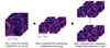 |
Fig. 1. Training stages of extended LDL. We first trained the base LDL parameters on the large volumes available for the fiducial model (CAMELS/CV) at z = 0.21. We then conditioned the LDL parameters on the cosmological and astrophysical parameters using the numerous boxes from the CAMELS/LH set. While the ne model performs equally at all redshifts, the T emulator has to be retrained separately at all available redshifts. |
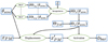 |
Fig. 2. Scheme of extended LDL. Blue rectangles denote quantities and green ovals denote transformations. The bottom row is the base LDL from Dai & Seljak (2021). Our extensions allow the baryon pasting to be conditioned on simulation parameters as well as on theredshift. |
2.3. Simulation-based pipeline
We used the extended LDL to produce mock X-ray observations. We generated 20 deg2 light cones extending from z = 0.1 out to z = 0.5. These boundaries are due to a current limitation of our code, which does not yet support parallelisation of one simulation over several GPUs. As a result, we tuned the redshift range so that one simulation almost fills up the memory of a 32Go V100 GPU. One light cone is made of 12 adjacent periodic boxes of equal co-moving size, each one evolved with different random initial conditions at z = 99. The depth of the boxes varies with Ωm, and so the number of particles and voxels. Several light cones profiles are displayed in Figure 4. We evolve DMO fields with JAXPM and then painted the electron number density and the temperature with the extended LDL in voxels, all at a fixed resolution of 0.39h−1 Mpc.
The detection was performed independently on each map along the line of sight, over the total [0.5–1]+[1–2] energy band, using sep (Barbary 2016), a python implementation of SExtractor (Bertin & Arnouts 1996). For each detected object, we summed the CR[0.5 − 2] in its corresponding segmentation mask to obtain the integrated source CR. We retained all sources with CR[0.5 − 2] > 0.02 c/s, a flux limit that gives a density of cluster similar to the XXL C1 sample with the traditional forward model (Kosiba et al. 2025). For the selected sources, we computed their hardness ratios HR ≡ CR[1 − 2]/CR[0.5 − 1], a tracer of the cluster temperature and redshift. The adopted detection method is simple and could be upgraded to better reproduce real-observation processing (Pacaud et al. 2006), but is sufficient for the purpose of this proof-of-concept paper. Moreover, we mention that projection effects within a light cone are ignored in the detection process. We omitted the Poisson noise and neglected measurement errors on the CR and the HR, which has an impact on the number of objects detected. Some X-ray mocks are shown as examples in Figure 3. We finally regrouped the objects detected in ten independent lightcones to populate a 3D XOD, representative of a 200 deg2 and 10ks depth survey carried out with XMM-Newton. These XODs serve as the input statistic used during the inference.
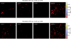 |
Fig. 3. X-ray mock examples generated with extended LDL. Each row consists of the same light cone, with three boxes individually projected (left and middle) and the full projected light cone with its 12 simulations boxes (right). The CR corresponds to a XMM-Newton EPIC/mos1+mos2+pn count-rate (without Poisson noise) in the [0.5–2] keV band. |
 |
Fig. 4. Light-cone profiles for Ωm = 0.1, 0.3, 0.5 (resp. black, green, blue), intersected with the 20 deg2 observed region (dashed red cone). The 12 adjacent periodic boxes (dashed rectangles) in each light cone share the same co-moving dimensions. Also shown with stars are the redshifts (0.1, 0.2, 0.3, 0.4, 0.5) for each cosmology. |
We then computed the X-ray emission of each voxel. We assumed the intracluster gas was at a fixed metallicity of Z = 0.3Z⊙, and we used pyatomDB2 (Foster et al. 2012) to compute the bremsstrahlung emission spectrum. We developed xrayflux3, a convenient wrapper of pyatomDB that redshifts the spectra and convolves them by the instrument response. We used the XMM-Newton/EPIC response files, and we obtain count rates (CRs) in the bands [0.5–1] and [1–2] keV (observer frame), similarly to the framework used in the XXL Survey (Pierre et al. 2016). We did not model the galactic absorption, which is negligible when observing far enough from the galactic plane, as in XXL. For wider surveys, the modelling of the galactic absorption and of its variations across the covered area would be necessary (as for instance in Clerc et al. 2024). For simplicity, we do not include X-ray AGNs in the field, and we did not add Poisson noise to the photon counts. We projected the boxes along the line of sight separately and obtained 12 X-ray maps in each energy band, with a resolution of ∼1′.
This pipeline benefits from GPU acceleration until the detection step. Thanks to the PM simulations and the extended LDL, the whole generation process is very fast: ∼100 seconds are required to produce an XOD of a 200 deg2 survey, evolving a total of ∼109 DM particles.
3. Simulation-based cosmological inference
We describe a fast forward model based on cosmological simulations in the previous section. From this, analytical scaling relations are required to write the likelihood and to perform a traditional inference scheme such as a MCMC one. However, here, our simulations do not provide us with such scaling relations, and this prevents us from using an explicit likelihood. We therefore turned to simulation-based inference (SBI), a new field that emerged thanks to the advances in ML. Specifically, the use of neural density estimators (such as Bishop 1994; Jimenez Rezende & Mohamed 2016) enabled us to learn the probability density of interest. We now detail our approach, which was inspired by Kosiba et al. (2025).
3.1. Neural compression
As a first step, we performed neural compression on our XODs. The motivation for this is that SBI techniques usually work better on low-dimension statistics. We built a convolutional neural network with ResNet blocks (He et al. 2015), which takes the XODs x as input (with the redshift dimension as image channels) and outputs the neural compression y (a vector containing 6 scalars, the size of the simulation parameter vector θsim). We used a rather shallow architecture, with four ResNet blocks (3 convolution layers each) followed by one MLP (3 dense layers). We trained our CNN to retrieve the latter using a mean-squared error loss, a choice that can lead to biased posterior (Lanzieri et al. 2025; Jeffrey et al. 2021). As we did not apply the posterior estimation on real data and were primarily interested by the size of the constraints, this choice is not critical in this work.
We generate a large sample of 48 000 XODs with our pipeline, each one with a random set of simulation parameters. 32 000 XODs were used for the training, 4000 for the validation, and 4000 for testing. The remaining 8000 are used for the inference. We applied a normalisation on both the input XODs and the target parameters such that all fields seen by the ResNet are between 0 and 1. The generation of these datasets necessitates ∼2000hGPU, while the ResNet training and the inference only requires ∼1hGPU.
3.2. Neural posterior estimation
We then directly learned the posterior from the compressed statistics y, using the neural posterior estimation (NPE) technique (Papamakarios & Murray 2016). Unlike the neural likelihood estimation (NLE, Wood 2010), the NPE is amortised, meaning that we do not need to retrain our density estimator when we have a new observation y0. One downside of the NPE is that the prior is encoded in the learnt density, and hence cannot be easily changed. We used a mixture density network (MDN) to emulate the conditional posterior qφ(θ ∣ y), with φ being the MDN weights. We used the package sbi (Tejero-Cantero et al. 2020) to train an MDN instantiated with ten Gaussian components. For any y0 unseen during training, we were able to directly sample the neural posterior qφ(θ ∣ y = y0), show the high-density regions, and compute the uncertainties on each parameter.
4. Results
We first introduce the analytical forward model to be compared with the simulation-based pipeline developed in this work. In a second step, we study the fidelity of the LDL surrogate simulations relatively to the original hydrodynamical CAMELS. Afterwards, we look at the possibility of obtaining posteriors using this accelerated, simulation-based forward model.
4.1. Analytical modelling
As a baseline for comparison, we considered a traditional forward model that uses empirical scaling relations. In this paper, we are mainly interested in comparing the two methods on the inference task, but we also compare the observed dN/dz in order to quantify the general level of realism of our model. We keep the fiducial values of Ωm and σ8 from Table 1, and retain the Planck Collaboration VI (2020) values for the remaining cosmological parameters. We then express the number counts in the mass-redshift plane with the HMF from Tinker et al. (2008). We used the scaling relations from Pacaud et al. (2018) to obtain the cluster temperature and luminosity, following which we computed the measured X-ray flux with the XMM-Newton/EPIC instruments using XSPEC (Arnaud 1996). As in the previous Section, we only kept the objects with a CR larger than CR[0.5 − 2],lim = 0.02 c/s. This does not ensure the selection functions are strictly equal between both models, as the detection algorithm used on the simulations may induce some artefacts. We finally obtain the source density in the (CR, HR, z) space, which we multiplied by the survey solid angle, 200 deg2. We compared the simulation-based and analytical forward models in Table 2.
Comparison of different number-count modelling in this work and from the literature.
4.2. Extended LDL results
Although we are interested in clusters, we first take a look at the raw LDL results, i.e. at the voxel level. In Figure 5, we show the voxel electron number density as a function of the DM density to critical density ratio, for the test simulations of the CV set, both for the original hydrodynamical boxes and their LDL-predicted counterparts. The dispersion of the LDL prediction is (1.90 ± 0.08)×10−5 cm−3 at the voxel level, which is significantly less than that of the original values, (3.0 ± 0.1)×10−5 cm−3 (over 5σ statistical difference). This means that our model does not fully capture the diversity of ne at a given ρDM/ρc. Moreover, we fitted and display power laws for both the target and predicted voxels. We computed the deviation of each voxel from the power law, and the correlation between the hydrodynamical and LDL deviations. The correlation coefficient is found to be 0.56, which indicates that the LDL voxels are not simply randomly dispersed around the mean power law. However, these results concern the properties of voxels only and do not yield much information on our primary focus (clusters), so we prevented ourselves from over-interpreting the raw LDL predictions.
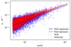 |
Fig. 5. Relation between electron number density, ne, and the DM density for the hydrodynamical simulations (blue crosses) and the LDL surrogate (red crosses) for the fiducial parameters and at z = 0.21. The blue and red lines denote the mean locus (respectively for the hydrodynamical and the LDL-predicted voxels). The voxel deviation from the mean for both methods is quite correlated (ρcorr = 0.56), but the LDL predictions do not reproduce the same scatter as in the originalsimulations. |
Secondly, we looked at the cluster results, using the procedure described in Sect. 2.3. Although we do not use explicit scaling relations in our modelling, in principle the cluster population in the CAMELS simulations should emulate implicit scaling relations, a physical consequence of the collapse of DM overdensities. Once again, relying on the test simulations from the CV set at z = 0.21, we computed the mock X-ray maps from both the original and the LDL simulations. We ran the detection on the ρDM/ρc maps, to avoid any bias towards the true or predicted structures in the CR maps. We compute the mass, the true CR and the predicted CR by integrating over the detection mask of each source. The mass measured here does not exactly relate to the spherical overdensity mass as in classical cluster studies. But as the detection uses a threshold of ρDM/ρc = 200, it can be considered as an approximation of M200c without the spherical assumption and including potential contaminants on the line of sight. Still, we can compare our hydrodynamical and LDL clusters since their mass estimates are consistent. In Figure 6, we first show the CR − M relation for each cluster set. Our LDL-emulated cluster sample reproduces the normalisation, slope and scatter of the clusters very well in CAMELS/CV. However, our approach does more than just recover the scaling relation; we again computed the deviation of each cluster CR to the mean relation and find that the LDL and true deviations are very well correlated (ρcorr = 0.88). This shows that, thanks to the 3D-modelling approach, our trained LDL is able to integrate some information from the cluster environments, and how this affects cluster properties. In that sense, our modelling is superior to an explicit and empirical scaling relation. We also computed the error on the prediction (see Figure 6, right panel), and find it to be two times smaller than the natural scatter of the CR − M relation. However, this study cannot be reproduced for the LH set, given that for one specific set of simulation parameters, we only have one (25h−1 Mpc)3 box, which does not provide sufficient statistics on clusters. This shows a limitation of the version of CAMELS we used here.
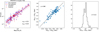 |
Fig. 6. CR − M scaling relation at z = 0.21 in CAMELS/IllustrisTNG simulations and in their LDL surrogate, for the fiducial model. These plots were done with the CV test set: 6 boxes with a volume of (50h−1 Mpc)3 each. Left: Direct comparison of hydrodynamical simulated clusters (blue crosses) and their LDL counterpart (red crosses). The plain lines and shaded region indicate respectively the mean relation and scatter for each method. The scaling relation is well reproduced by the LDL method. Middle: Deviation of hydrodynamical values and LDL prediction to the mean relation (blue points), and the 1:1 slope (dashed line). The strong correlation indicates that the LDL recovers more than just a scaling relation: it can learn why a specific cluster is over or under luminous, given its mass, thanks to its 3D DM distribution. Right: Histogram of CR prediction errors. At the cluster level, the LDL prediction appears unbiased, and with a scatter of 0.12 dex, smaller than the natural scatter of the CR − M relation. |
We compare the cluster number counts from simulation and analytical models in Figure 7. For our simulation-based model, we generated 48 surveys covering 50 deg2, with z ∈ [0.1, 0.5], and measured the redshift distribution in each of them. We obtain theoretical number counts with the analytical model presented in Section 4.1, for a survey with the same dimensions. We also display the observed distribution from the XXL Survey, although one should keep in mind that it is not directly comparable, because the XXL selection function is more complex than the simple CR cut we used. While the simulated and analytical distributions share the same peak position (at z = 0.2) and compatible number counts for z > 0.3, we observe a significant discrepancy at lower redshifts, where our simulation-based number count is larger than the explicit modelling: the total number of clusters with our LDL simulations is 40% higher than with the analytical model. This is surprising as we have previously shown that our LDL model reproduces the fiducial cluster population from CAMELS well. However, we have left several important questions. Firstly, it is possible that the X-ray luminosity of simulated clusters is not realistic enough. Pop et al. (2022) showed that the X-ray luminosity in IllustrisTNG clusters is slightly higher than that of observed samples, in particular for the core-excised luminosity. We also note in Pop et al. (2022) that the LX − M relation of IllustrisTNG clusters appears to be low scattered. Through selection effects, small differences in the simulated luminosities can cause notable changes in the dN/dz. In addition, we have no guarantee that the HMF arising from the CAMELS simulations is compatible with the functional fit from (Tinker et al. 2008). Notably, it is known that baryonic processes affect the HMF (Bocquet et al. 2016; Kugel et al. 2024). Aside from this consideration, we recall that we implemented very simple detection and property measurement processes, which are also likely to impact the number counts in terms of output. In this work, we focused on the LDL acceleration and SBI for cluster cosmology, so we leave these questions open for now. It will be necessary to consider them before applying our method to real data.
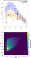 |
Fig. 7. Top: Redshift distribution of cluster counts for traditional forward model (with explicit scaling relations, orange histogram) and for the simulation-based model (with the LDL, blue histogram), here for a 50 deg2 survey extending from z = 0.1 to z = 0.5. The shaded regions display the 3σ Poisson standard deviation for each model. Also shown is the observed distribution of C1 clusters in the XXL Survey (dashed black histogram), however one should keep in mind that the selection function is in this case more complex than a simple flux cut. We stress that this Figure is not a goodness of fit: both models are calibrated independently. Bottom: Cluster population in CR–HR space for simulation-based model, also for a 50 deg2 survey extending from z = 0.1 to z = 0.5. The CR and HR in the simulation-based and scaling-relation-based models are computed differently; hence we did not compare their distributions. |
4.3. Posteriors
We now present the results of the simulation-based inference with the ResNet compressor and the NPE method. We recall that in the SBI steps, our models are trained and tested on the large dataset of XODs (48 000 cluster catalogues sampled) generated with the extended LDL and pipeline described in Section 2. We first look at the regression performance of the ResNet model, which was trained and tested on our simulated XOD dataset varying the six simulation parameters considered in this work, in Figure 8. The ResNet retrieves Ωm and σ8 well, as the points are distributed close to the 1:1 slope. The SN feedback parameters are also recovered, but with a larger scatter. However, the ResNet predictions are highly scattered for the AGN feedback parameters as currently implemented in CAMELS, and they present biases near the edge of the sampled prior (see Figure 8, bottom left and bottom right panels). This indicates that our forward model is not very sensitive to these parameters, at least under the XOD statistics and for a 200 deg2 survey. The weak response of our LDL model to the AGN feedback variations in fact stems from the CAMELS dataset itself. We discuss this point in Section 5.4.
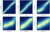 |
Fig. 8. Accuracy of ResNet regression for inferring Ωm, σ8, ASN1, AAGN1, ASN2 and AAGN2 from simulation-based XODs. The colour and contours show the shape of the density of points (arbitrary colour scale, all densities are normalised). The dashed line shows the 1:1 line (no error). We observe that the two cosmological parameters are well recovered. The SN feedback parameters are also rather well estimated, although with a stronger scatter. However, the ResNet struggles to retrieve the AGN feedback parameters, meaning that these parameters do not significantly influence our XOD statistics. |
Finally, we present the results of the NPE method. We used simulated XODs x0 that were used neither for the ResNet training nor its testing, and we used the ResNet to obtain their compressions y0. The compressions are in turn passed to the trained NPE, providing us with posterior estimations q(θ ∣ y = y0), marginalised over the feedback parameters. We show the 68% and 95% credibility regions on cosmology, marginalized over the feedback parameters, for 16 different y0 in Figure 9, where we simply excluded XODs simulated from parameters close to the border of the parameter space. We show, in addition, the position of the compression y0, and of the true underlying cosmological parameters θtrue. We stress that all θtrue shown are different. We add, in Appendix B, an analysis of the quality of our posteriors. This illustrates the viability of our model for a cosmological inference. The acceleration of the simulations with GPU resources and the LDL surrogate baryonification enables the creation of the datasets required by the SBI approach we used.
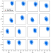 |
Fig. 9. NPE performed at different points in parameter space. XODs are produced from 200 deg2 X-ray surveys, selecting clusters with the flux cut CRlim = 0.02c/s. The posteriors (blue contours) are obtained with the NPE for XODs not seen during the ResNet or NPE trainings. A tested XOD x0 is compressed into a y0, the position of which in the parameter space is indicated by a red square. The green star shows the true parameters that were used to simulate x0. |
In Figure 9, the commonly observed degeneracy between σ8 and Ωm in cluster counts experiments appears notably weak. While this degeneracy typically arises from the role that σ8 and Ωm play in shaping the HMF, the impact of nuisance parameters on the degeneracy may vary between different models of X-ray cluster properties. In our framework, we tested this by comparing the inferred posteriors obtained with and without including feedback parameters in the analysis. For this purpose, we ran a new set of simulations with fixed astrophysics, reused our ResNet to convert the XODs into neural compressions, and finally retrained a posterior estimator conditioned solely on the cosmology. We took a fiducial diagram, x0, and passed it to both posterior models (one conditioned on all parameters and one conditioned only on cosmology), and we show the resulting contours in Figure 10. Our model retrieves a more pronounced degeneracy between σ8 and Ωm, with fixed feedback parameters. Interestingly, including them in the inference broadens the posterior, in particular along the transverse direction to thedegeneracy. We recall that feedback is also accounted for in a scaling-relation-based model, but through an empirical parametrisation that broadens the original Ωm–σ8 contour in a different manner.
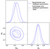 |
Fig. 10. Posteriors estimated from a fiducial XOD for different conditioning of NPE. The XOD is produced from a 200 deg2 X-ray survey, selecting clusters with the flux cut CRlim = 0.02 c/s. In plain blue we show a posterior marginalised on the feedback parameters, while in dashed blue we show a posterior from an NPE only conditioned on the cosmology. The vertical and horizontal lines recall the fiducial values used for generating the tested XOD. |
5. Discussion
5.1. Intrinsic degeneracies of the simulation-based and analytical models
To assess the relevance of our new modelling, we first studied the intrinsic degeneracies of both models. For the analytical forward model, we can explicitly write the likelihood. In writing an XOD as a set of expected number counts λi(θ) in bins of the (CR, HR, z) space, and if we assume that observed counts in different bins are independent and follow a Poisson distribution, we can express the Fisher matrix in the following manner:
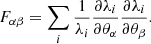 (8)
(8)
Under the assumption that the likelihood is Gaussian, the Fisher matrix can be inverted to obtain the optimal constraints achievable by the model. More details on the computation of the Fisher matrix can be found in Cerardi et al. (2024) and Kosiba et al. (2025).
In Figure 11 and 12, we show the full posteriors for the simulation-based and analytical models, respectively obtained through the NPE and Fisher analysis methods. An elongated contour indicates a degeneracy between parameters. Many clear degeneracies appear in the model with scaling relations; not only are the scaling relation coefficients degenerate between each other (e.g. αMT and γMT), they are also degenerate with the cosmological parameters (e.g. M0 and Ωm). This shows that even under our XOD statistic (which is superior to a representation in the mass redshift plane, see Clerc et al. 2012a), these parameters are hard to separate. We do not observe similar degeneracies for the simulation-based model. With the current set of parameters, only ASN1 and ASN2 seem slightly degenerate but, most importantly, none of the feedback parameters appear degenerate with cosmology. This is the consequence of our approach being based on feedback prescriptions describing the physical processes within the ICM. Our model carries inherent physical constraints on cluster observable properties. In this proof of concept, we assume that feedback models are correct (within the freedom given to the four feedback parameters), which introduces a lot of information in the inference.
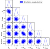 |
Fig. 11. Posteriors on cosmological and astrophysical parameters, using the simulation-based forward model and the NPE inference method. The tested diagram x0 is drawn from the fiducial model. XODs are produced from 200 deg2 X-ray surveys, selecting clusters with the flux cut CRlim = 0.02c/s. |
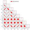 |
Fig. 12. Posteriors on cosmological and nuisance parameters, using the analytical forward model and the Fisher analysis, with explicit scaling relations. We observe that many pairs of parameters are degenerate (elongated contours), denoting the ill-parametrisation of this model. The simulation-based forward model does not show this behaviour in Figure 11. XODs are produced from 200 deg2 X-ray surveys, selecting clusters with the flux cut CRlim = 0.02c/s. |
5.2. Towards a universal parametrisation
The analytical modelling uses a set of empirical scaling relations that has to be well adapted to the chosen study; that is because there is no general modelling available (see i.e. the different references in Table 2). Depending on the observables and on the characteristics (more or less massive, more or less distant) of the detected sources, one would change the number of scaling relations used and the number of free parameters to best fit the data (see the compilation in Table 2). For instance, the eRASS1 analysis does not use the HR (thus, no L − T or M − T relation is needed), but it does include the optical richness λ (so an extra relation, M − λ, has to be modelled), and several model parameters have a redshift dependence at the cost of extra nuisance parameters. As the parameters of our simulation-based model are related to the physical processes in the ICM, we do not need need to change our parametrisation for a different set of observables. In Figure 13, we show the contours obtained if we run the analysis by simply removing one or two dimensions in the (CR, HR, z) space. The contours are slightly broadened because of the loss of information, but the constraints are still informative. This can also be seen in the Table 3, which compares the relative Figure of merit of these posteriors. Clerc et al. (2012a) found that the redshift distribution struggles to constrain cosmology, because of degeneracies between parameters that the CR–HR representation is able to break. With our simulation-based model trained on astrophysical processes, the dn/dz statistics provides constraints that are comparable to those from the CR–HR space. This prediction is quite different from that by Clerc et al. (2012a) (Figure 12) and suggests, that because our set of (non-cosmological) priors is more physically motivated than theirs, our scaling-relation-independent modelling of cluster properties is less degenerate. Our approach thus seems to ’naturally’ exclude entire unphysical regions of the coefficient-cosmology space, which were left open in the approach relying on scaling relations with priors. However, in this comparison, one has to consider that Clerc et al. (2012a) implemented measurement errors in the CR-HR space and had one more free cosmological parameter (w0), which led to additional degeneracies.
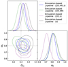 |
Fig. 13. Cosmological posteriors obtained with simulation-based forward model and NPE. We trained the NPE for several statistics: the full (CR, HR, z) XOD (blue contours), the (CR, HR) number counts (dashed green), the (CR, z) number counts (dashed purple) and only the z distribution (dashed black). The same simulations, forward model, and parametrisation were used, and we still recover informative constraints for all these cases. |
Performances of different test statistics with simulation-based model.
5.3. Scaling relations conditioned on astrophysical parameters
In Section 4.2, we study the CR–M scaling relations emulated in our simulations under the fiducial set of parameters. This provides a new way of modelling cluster number counts; we can use our simulation-based model to compute new scaling-relation coefficients when changing the cosmological and the feedback parameters. In Figure 14, we track the changes of the slope and scatter (two coefficients that have theoretical predictions, from which actual values may differ because of non-gravitational processes) of the CR–M law when changing ASN1 and ASN2. We simulated, for each set of parameters, 16 simulations with a volume of (150 × 150 × 50) h−3 Mpc3, at z = 0.21, projected on the last dimension. This represents 144 times the volume of one CAMELS simulation from the CV set, and hence provides us with many cluster detections to compute scaling relations. In the top panel of Figure 14, showing the variations of αCR − M, the error bars are large, and hence only general trends can be retained. We see that the parameter slightly increases (decreases) with increasing (decreasing) ASN1 (ASN2). This response of the slope parameter could explain the weak negative degeneracy observed in the full simulation-based posterior (Figure 11) in the ASN1–ASN2 region. The bottom panel of Figure 14 shows a cross effect of the two SN feedback parameters on the slope. At low values of ASN1, σCR − M is strongly affected when ASN2 is varied. Interestingly, this behaviour does not appear for high ASN1 values, at least for the current level of uncertainty on the data points. In Appendix C, we provide a more complete view of the dependence of the scaling relations on the simulation parameters, including Ωm and σ8.
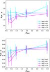 |
Fig. 14. CR–M relation coefficients as a function of simulation parameters, for large volumes emulated at z = 0.21. The x-axis varies the ASN1 feedback parameter, while the line colour denotes a change in ASN2. The top and bottom panels respectively show the variations of the slope αCR − M and of the intrinsic scatter σCR − M. The error bars show the interval covering 68% of the measured point around the median. The lines have been slightly shifted horizontally to improve readability. |
With a simulation-based model that considers all relevant astrophysical parameters from simulations, we could build an emulator of plausible scaling relations as a function of cosmological and astrophysical parameters and, subsequently, forward model cluster counts with these emulated scaling relations. This way, we would be able to sample the cosmological and astrophysical parameter space, avoiding forbidden regions and the degenerate parametrisation of the scaling relations. This would also allow an important increase in speed, as XODs created with emulated scaling relations would require fewer computational resources than with the simulation-based model. Traditional inference techniques would be available for this type of forward model, as we would obtain theoretical number counts instead of Poisson realisations of XODs. However, we would lose the spatial information on the cluster properties within the cosmic network (not used in this paper).
5.4. Potential application to real data
In order to apply our method for an inference with real data, several points should be carefully considered. The third question raised in the introduction, related to the realism of hydrodynamical simulations, becomes critical here. In Section 4.2, we note that our simulation-based model appears to predict more clusters than the analytical method. We ruled out a systematic error from the LDL prediction, as the luminosity mass relation for groups and clusters (Figure 6) is well reproduced. Candidates for this discrepancy might be the X-ray properties emulated in the CAMELS/IllustrisTNG simulations. As a result of the CAMELS implementation, SN and AGNs are tuned to provide realistic star formation histories, but not the overall properties of the X-ray cluster population. We hence highlight the importance of calibrating the sub-grid physical models on cluster-related observables. Besides the simulations used for calibration, another critical point is the detection method. For a forward model, it is important to integrate the same biases as the ones inherent to the processing of real data. Given that our method produces mock X-ray observations, the straightforward solution is to apply the same detection pipeline on both the real and mock data. To do this, some simplifications taken here have to be dropped; it becomes necessary to include AGN contaminants, CCD defaults, realistic diffuse and proton backgrounds, and a Poisson noise on the pixels photon counts. Concerning the measurement, error models are needed for a scaling-relation-based modelling (e.g. in Garrel et al. 2022), but not in a simulation-based modelling. Indeed, if the mocks and the detection are fully coherent with the observed data, the measurement errors would be encoded in the simulation output. As a result, we would not need an external model for that, as we do for a classical analysis.
A second improvement is expected regarding the simulations that serve to train the extended LDL. Villaescusa-Navarro et al. (2021), for instance found that the star formation rate density in the original CAMELS was not very sensitive to changes in the two selected AGN parameters that varied (only for Illustris/TNG). In addition, we also looked at the trend between ne, T and ρDM/ρc, at the voxel level in the CAMELS 1P set, which varies only one parameter at a time. We find that the gas properties are more affected by the SN parameters than by the AGN feedback. This could explain why our extended LDL is not very sensitive to these parameters. The surprising strong impact of SN feedback is in fact indirect: the coupling between SN and AGN feedback effectively tempers the latter, explaining the opposite trend from increased AGN activity (Tillman et al. 2023; Medlock et al. 2025). New versions of CAMELS simulations are being run that include the variations of additional physical parameters. More AGN feedback parameters will be implemented, specifically the threshold mass triggering the AGN kinetic feedback mode, a parameter that is known to significantly impact the X-ray luminosity of extragalactic gas (Truong et al. 2021). As a result, the extended LDL could be conditioned on parameters that effectively impact X-ray observables, and the learnt posterior could be marginalised on them. It will be necessary to test our approach under this new configuration to assess whether the additional parameters introduce degeneracies with the cosmology.
Another important asset of this new CAMELS dataset is the increase of the simulated box size, firstly to (50h−1 Mpc)3 and later to (100h−1 Mpc)3. This will first form more clusters and more massive ones, leading to more training samples for the LDL approach. Also, we only tested the fidelity of LDL-emulated scaling relations on the fiducial model, because the small boxes in the LH set only produce a handful of groups and lightweight clusters and do not provide us with sufficient statistics to compute scaling relations. The larger boxes of the next CAMELS iteration will provide us with more statistics. It could represent an opportunity to analyse the LDL generated clusters for non-fiducial sets of parameters. In addition, training and testing the extended LDL on more massive clusters will improve the consistency of our method when applied to bright cluster samples.
Another necessary improvement is related to the computational resources. Our approach can only currently run on a single GPU, which drastically limits the number of particles in a simulation. Here, the limiting factor has been the simulated volumes for the light-cone creation. This set the resolution of the LDL emulation, and hence we downgraded the CAMELS/IllustrisTNG simulations accordingly. A current work (Kabalan et al., in prep.) aims to parallelise critical parts of our simulations, which will eventually allow us to improve the resolution of our X-ray mocks. This is of particular importance as cluster cores can exhibit very diverse emission characteristics, and because the matter distribution in clusters contains information on the accretion and merger history of a given cluster.
6. Conclusions
In this paper, we present a novel approach to forward modelling cluster number counts in deep X-ray surveys. We used cosmological simulations, which integrate the dynamical and baryonic processes affecting the cluster luminosities. We have developed an accelerated baryonification technique by extending the LDL approach. The LDL uses particle displacements from corrections to the gravitational potential and non-linear activation to transform a DMO field into a targeted baryonic property field. As such, it is motivated by physical arguments and simpler than deep generative models. We allowed the baryonic properties to be conditioned on cosmology and on the feedback parameters. Moreover, our baryon pasting also depends on redshift. We adopted a novel, flexible Fourier filter to implement the LDL model and, subsequently, derived the cluster properties down to X-ray observables (i.e. XMM countrates in several bands). We created a large number of light cones (0.1 < z < 0.5, 200 deg2) to perform simulation-based cosmological inference for the cluster population in the CR-HR-z parameter space. We compared our results with the analytical approach.
Our method not only avoids inference on cosmology-dependent measurements (such as mass and luminosity), but also bypasses the use of empirical scaling relations to model the X-ray cluster properties. We now examine its impact on the three key questions raised in the introduction:
-
Accuracy of a fast ML emulator. We demonstrated that our extended LDL model was able to reproduce the cluster population from the original simulations, for the fiducial parameters. Moreover, our model does more than just recover the statistical properties of the population, it also partially captures the specificity of each individual cluster. In that sense, our modelling is superior to an approach based on scaling relations. However, due to the lack of simulated volume for non-fiducial parameters, we cannot run the same test in the whole parameter space. Improvements in the emulator resolution could help fix the remaining uncertainty on the X-ray fluxes at the individual cluster level. The availability of larger simulation boxes for some regions of the parameter space would help both the training and the testing of our model. The upcoming versions of CAMELS will satisfy this requirement. We recall that we chose a physics-based, lightweight ML approach. Conversely, one could try deep neural architecture to perform the baryonification, but at the cost of interpretability. It would be very informative to assess which approach performs better.
-
Viability for cosmological inference. Our fast baryonification method reduces the computational cost of a simulation-based forward model and thus enables cosmological inference. Compared to the analytical modelling, our approach is less degenerate and allows us to infer nuisance parameters that have a more physical meaning than scaling relation coefficients. Our parametrisation is indeed directly linked to well-identified astrophysical processes, and hence it is in principle more universal: it is insensitive to changes in the survey design or in the chosen summary statistics. Nonetheless, we can only leave free the parameters that are varied in the original CAMELS dataset, and it could be important to marginalise over other simulation parameters that are here fixed. Once again, the future developments of CAMELS will offer the opportunity to enlarge the conditioning of our extended LDL model.
-
Realism of the hydrodynamical simulations. Although this is not the main issue targeted in this work, the 40% difference between the simulation-based and analytical number counts may suggest a lack of realism. We question either the realism of the simulations, the fiducial values chosen for the feedback parameters, or the implementation of the retroaction mechanisms themselves. However, the gap we observe could also arise from our simplified cluster detection and characterisation process. Both, upgraded physics prescriptions in the hydrodynamical simulations and a more realistic detection chain will be necessary to apply our method to observed cluster samples. Although the output resolution of the simulations is not a critical point for our goals, the resolution of the hydrodynamic solver may well play a critical role in the realisms of the simulations.
Further work will be dedicated to a deeper analysis of the clusters emulated by the extended LDL, in order to characterise their profiles. We also plan to investigate discrepancies with the observational number counts by upgrading the production of the X-ray mocks. Regarding the fast baryon pasting approach, we will leverage the new large simulation sets in CAMELS to improve our analysis of the conditioning step. This will also allow us to more accurately map the scaling-relation coefficients as a function of the physical parameters (here SN and AGN feedback) as sketched in Figure 14. Consequently, we will be able to identify regions of the cosmology-coefficient space that are a priori forbidden by cluster physics. This would provide a novel approach to setting priors on the coefficients.
During the review process of this article, other works on SBI for cluster cosmology have been made available on arXiv (Zubeldia et al. 2025; Regamey et al. 2025, respectively for SZ and X-ray cluster samples). This demonstrates the growing interest in this new class of inference methods for cluster cosmology. However, these approaches differ from ours as they both employ scaling relations to forward model cluster properties.
Our simulation-based forward approach opens new avenues for implicit modelling and inference in cluster cosmology. In particular, when we are in a position to satisfactorily reproduce the observable properties of each individual cluster, the X-ray mapping will implicitly carry a lot of supplementary information relative to cluster environments and histories. This could in turn be implemented in the cosmological inference in terms of new observables. Hence, we can think of switching from CR-HR-z to a full spatial mapping of the cluster population in the form of CR-HR-z-x-y (x = RA, y = Dec). This would allow us to combine the current XOD with information comparable to the 2 pt-correlation function, but providing much more stringent constraints, since the X-ray cluster properties would be related to their location within the cosmic network. In this way, we anticipate that the new 5D summary statistics would exhaust the cosmological potential of an X-ray cluster survey, and remove most of the degeneracy in cluster cosmology. Joint modelling of other cosmological probes along with clusters is also a possibility within this framework, and it promises to break degeneracies between nuisance and cosmological parameters (Omori 2024).
Acknowledgments
The authors thank Camila Correa, Jean Ballet, Nicolas Clerc and Daisuke Nagai for relevant discussions around this work. The authors also thank the referee for insightful comments on this work. This work was granted access to the HPC resources of IDRIS under the allocations 2023-AD011013487 and 2024-AD011013487R2 made by GENCI. NC is grateful to the IDRIS technical team for their support on the Jean-Zay computational resources. NC thanks Shy Genel and Francisco Villaescusa-Navarro for sharing the CAMELS CV50 simulations. NC thanks Marine Lafitte for graphical help on the Figures.
References
- Abazajian, K., Addison, G., Adshead, P., et al. 2019, ArXiv e-prints [arXiv:1907.04473] [Google Scholar]
- Adami, C., Giles, P., Koulouridis, E., et al. 2018, A&A, 620, A5 [NASA ADS] [CrossRef] [EDP Sciences] [Google Scholar]
- Arnaud, K. A. 1996, ASP Conf. Ser., 101, 17 [Google Scholar]
- Arnaud, M., Pratt, G. W., Piffaretti, R., et al. 2010, A&A, 517, A92 [CrossRef] [EDP Sciences] [Google Scholar]
- Bahar, Y. E., Bulbul, E., Clerc, N., et al. 2022, A&A, 661, A7 [NASA ADS] [CrossRef] [EDP Sciences] [Google Scholar]
- Barbary, K. 2016, JOSS, 1, 58 [Google Scholar]
- Bertin, E., & Arnouts, S. 1996, A&AS, 117, 393 [NASA ADS] [CrossRef] [EDP Sciences] [Google Scholar]
- Bishop, C. M. 1994, Mixture density networks (Birmingham: Aston University) [Google Scholar]
- Bocquet, S., Saro, A., Dolag, K., & Mohr, J. J. 2016, MNRAS, 456, 2361 [Google Scholar]
- Bocquet, S., Dietrich, J. P., Schrabback, T., et al. 2019, ApJ, 878, 55 [Google Scholar]
- Bulbul, E., Chiu, I. N., Mohr, J. J., et al. 2019, ApJ, 871, 50 [Google Scholar]
- Cerardi, N., Pierre, M., Valageas, P., Garrel, C., & Pacaud, F. 2024, A&A, 682, A138 [NASA ADS] [CrossRef] [EDP Sciences] [Google Scholar]
- Clerc, N., Pierre, M., Pacaud, F., & Sadibekova, T. 2012a, MNRAS, 423, 3545 [NASA ADS] [CrossRef] [Google Scholar]
- Clerc, N., Sadibekova, T., Pierre, M., et al. 2012b, MNRAS, 423, 3561 [NASA ADS] [CrossRef] [Google Scholar]
- Clerc, N., Comparat, J., Seppi, R., et al. 2024, A&A, 687, A238 [NASA ADS] [CrossRef] [EDP Sciences] [Google Scholar]
- Dai, B., & Seljak, U. 2021, PNAS, 118, e2020324118 [Google Scholar]
- Dai, B., Feng, Y., & Seljak, U. 2018, JCAP, 2018, 009 [Google Scholar]
- DES and SPT Collaborations (Bocquet, S., et al.) 2025, Phys. Rev. D, 111, 063533 [Google Scholar]
- DESI Collaboration (Abareshi, B., et al.) 2022, AJ, 164, 207 [NASA ADS] [CrossRef] [Google Scholar]
- Foster, A. R., Ji, L., Smith, R. K., & Brickhouse, N. S. 2012, ApJ, 756, 128 [Google Scholar]
- Garrel, C., Pierre, M., Valageas, P., et al. 2022, A&A, 663, A3 [NASA ADS] [CrossRef] [EDP Sciences] [Google Scholar]
- Ghirardini, V., Bulbul, E., Artis, E., et al. 2024, A&A, 689, A298 [NASA ADS] [CrossRef] [EDP Sciences] [Google Scholar]
- Hassan, S., Villaescusa-Navarro, F., Wandelt, B., et al. 2022, ApJ, 937, 83 [NASA ADS] [CrossRef] [Google Scholar]
- He, K., Zhang, X., Ren, S., & Sun, J. 2015, ArXiv e-prints [arXiv:1512.03385] [Google Scholar]
- Henry, J. P., Gioia, I. M., Maccacaro, T., et al. 1992, ApJ, 386, 408 [NASA ADS] [CrossRef] [Google Scholar]
- Ivezic, Z., Kahn, S. M., Tyson, J. A., et al. 2019, ApJ, 873, 111 [NASA ADS] [CrossRef] [Google Scholar]
- Jeffrey, N., Alsing, J., & Lanusse, F. 2021, MNRAS, 501, 954 [Google Scholar]
- Jimenez Rezende, D., & Mohamed, S. 2016, ArXiv e-prints [arXiv:1505.05770] [Google Scholar]
- Kaiser, N. 1986, MNRAS, 222, 323 [Google Scholar]
- Kosiba, M., Cerardi, N., Pierre, M., et al. 2025, A&A, 693, A46 [NASA ADS] [CrossRef] [EDP Sciences] [Google Scholar]
- Kugel, R., Schaye, J., Schaller, M., et al. 2024, MNRAS, 534, 2378 [Google Scholar]
- Lanzieri, D., Lanusse, F., & Starck, J.-L. 2022, Machine Learning for Astrophysics, Proc. 39th International Conference on Machine Learning (ICML 2022), https://ml4astro.github.io/icml2022, 60 [Google Scholar]
- Lanzieri, D., Zeghal, J., Makinen, T. L., et al. 2025, A&A, 697, A162 [NASA ADS] [CrossRef] [EDP Sciences] [Google Scholar]
- Lee, M. E., Genel, S., Wandelt, B. D., et al. 2024, ApJ, 968, 11 [NASA ADS] [CrossRef] [Google Scholar]
- Maartens, R., Abdalla, F. B., Jarvis, M., & Santos, M. G. 2015, in PoS(AASKA14), 215, 016 [Google Scholar]
- Mantz, A., Allen, S. W., Rapetti, D., & Ebeling, H. 2010, MNRAS, 406, 1759 [NASA ADS] [Google Scholar]
- Mantz, A. B., Allen, S. W., Morris, R. G., et al. 2016, MNRAS, 463, 3582 [NASA ADS] [CrossRef] [Google Scholar]
- Maughan, B. J., Giles, P. A., Randall, S. W., Jones, C., & Forman, W. R. 2012, MNRAS, 421, 1583 [Google Scholar]
- Medlock, I., Neufeld, C., Nagai, D., et al. 2025, ApJ, 980, 61 [Google Scholar]
- Mellier, Y., Abdurro’uf, A., Barroso, J. A. A., et al. 2025, A&A, 697, A1 [Google Scholar]
- Nandra, K., Barret, D., Barcons, X., et al. 2013, ArXiv e-prints [arXiv:1306.2307] [Google Scholar]
- Nelson, D., Springel, V., Pillepich, A., et al. 2019, Computat. Astrophys. Cosmol., 6, 2 [NASA ADS] [CrossRef] [Google Scholar]
- Ni, Y., Genel, S., Anglés-Alcázar, D., et al. 2023, ApJ, 959, 136 [NASA ADS] [CrossRef] [Google Scholar]
- Omori, Y. 2024, MNRAS, 530, 5030 [NASA ADS] [CrossRef] [Google Scholar]
- Pacaud, F., Pierre, M., Refregier, A., et al. 2006, MNRAS, 372, 578 [NASA ADS] [CrossRef] [Google Scholar]
- Pacaud, F., Pierre, M., Melin, J.-B., et al. 2018, A&A, 620, A10 [NASA ADS] [CrossRef] [EDP Sciences] [Google Scholar]
- Papamakarios, G., & Murray, I. 2016, in NeurIPS (Curran Associates, Inc.), 29 [Google Scholar]
- Perlmutter, S., Turner, M. S., & White, M. 1999, Phys. Rev. Lett., 83, 670 [CrossRef] [Google Scholar]
- Pierre, M., Pacaud, F., Adami, C., et al. 2016, A&A, 592, A1 [NASA ADS] [CrossRef] [EDP Sciences] [Google Scholar]
- Pillepich, A., Springel, V., Nelson, D., et al. 2018, MNRAS, 473, 4077 [Google Scholar]
- Planck Collaboration, VI. 2020, A&A, 641, A6 [NASA ADS] [CrossRef] [EDP Sciences] [Google Scholar]
- Pop, A. R., Hernquist, L., Nagai, D., et al. 2022, ArXiv e-prints [arXiv:2205.11528] [Google Scholar]
- Predehl, P., Andritschke, R., Arefiev, V., et al. 2021, A&A, 647, A1 [EDP Sciences] [Google Scholar]
- Regamey, M., Eckert, D., Seppi, R., et al. 2025, A&A, submitted [arXiv:2506.05457] [Google Scholar]
- Riess, A. G., Filippenko, A. V., Challis, P., et al. 1998, AJ, 116, 1009 [Google Scholar]
- Sobrin, J. A., Anderson, A. J., Bender, A. N., et al. 2022, ApJS, 258, 42 [NASA ADS] [CrossRef] [Google Scholar]
- Tejero-Cantero, A., Boelts, J., Deistler, M., et al. 2020, JOSS, 5, 2505 [Google Scholar]
- Tillman, M. T., Burkhart, B., Tonnesen, S., et al. 2023, AJ, 166, 228 [Google Scholar]
- Tinker, J., Kravtsov, A. V., Klypin, A., et al. 2008, ApJ, 688, 709 [Google Scholar]
- Truong, N., Pillepich, A., & Werner, N. 2021, MNRAS, 501, 2210 [NASA ADS] [CrossRef] [Google Scholar]
- Vikhlinin, A., Kravtsov, A. V., Burenin, R. A., et al. 2009, ApJ, 692, 1060 [Google Scholar]
- Villaescusa-Navarro, F., Anglés-Alcázar, D., Genel, S., et al. 2021, ApJ, 915, 71 [NASA ADS] [CrossRef] [Google Scholar]
- Villaescusa-Navarro, F., Genel, S., Anglés-Alcázar, D., et al. 2022, ApJS, 259, 61 [NASA ADS] [CrossRef] [Google Scholar]
- Villaescusa-Navarro, F., Genel, S., Anglés-Alcázar, D., et al. 2023, ApJS, 265, 54 [NASA ADS] [CrossRef] [Google Scholar]
- Wood, S. N. 2010, Nature, 466, 1102 [Google Scholar]
- Zubeldia, I., Bolliet, B., Challinor, A., & Handley, W. 2025, ArXiv e-prints [arXiv:2504.10230] [Google Scholar]
- Zwicky, F. 1933, Helvetica Phys. Acta, 6, 110 [NASA ADS] [Google Scholar]
Appendix A: Sampling distribution for the simulation parameters
We used the CAMELS simulation suite to train and test our extended LDL method. In Figure A.1, we show the parameter distribution for each of six varied parameters, in the CAMELS/LH set. For completeness, we show both the distribution for the full suite (dotted lines, 1000 samples), and for the subset we used (plain lines, 499 samples). We do not observe a specific concentration of the simulated boxes parameters in the 1D distributions. By construction, the LH set samples parameters mimicking a uniform (or log-uniform for the feedback parameters) distribution. Our subset, even if it divides the density of points by a factor of 2, still conserves a rather regular sampling.
 |
Fig. A.1. 1D distributions of the simulations parameters in the CAMELS/LH suite. Dotted lines indicate the full suite (1000 boxes), while the plain lines show the actual distribution of the subset we used (499 boxes). |
Appendix B: Quality of the posteriors
We assessed the quality of the 1D posteriors on the cosmology. We began with 500 XODs x0 not seen during the ResNet and NPE trainings, which we compressed into y0. We followingly obtained 500 6-dimensional posteriors qφ(θ ∣ y = y0). We then obtained the 1D posteriors over Ωm and σ8 by marginalising over the other parameters. We computed the 1D rank for both Ωm and σ8:
 (B.1)
(B.1)
with p the 1D marginalised posterior. We show the distribution of r(θtrue, y0), for both parameters, in Figure B.1. A flat trend indicates no bias, while a slope reveals a bias. A concavity (resp. convexity) denotes an underconfidence (overconfidence) of the posterior. The linear trend for each plot indicates that our posteriors have the right size. However, the negative slope for Ωm shows that we are biased on this parameters, which could be explained by the MSE loss in the regression. Lanzieri et al. (2025) have for instance found that this loss function can induce a biased posterior. We devote to a further study the exploration of other SBI methods within our framework.
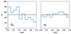 |
Fig. B.1. Ranks of the true Ωm (left) and σ8 (right) in the 1D marginalized posteriors. We have tested 500 different compressions y0, leading to the distributions represented in the blue histograms. If the posteriors are unbiased and with the proper width, the observed distribution should be pproximately flat (dashed black line). This is the case for σ8. However, Ωm exhibits a negative slope that indicate a bias, but still an appropriate posterior size (no apparent curvature). |
Appendix C: Deeper insights into the CR − M scaling relation coefficients as a function of simulation parameters
 |
Fig. C.1. 4D view of the dependance of the scaling relation coefficients on the simulation parameters. The marker size denotes the value of the scaling relation slope, and the marker color represents its dispersion. Both quantities are normalized with respect to the scaling relation of the fiducial model (central point). Top: Variation of the CR-M slope and scatter when varying Ωm, σ8, sampled on a linear grid. Bottom: Variation of the CR-M slope and scatter when varying ASN1 and ASN2, sampled on a logarithmic grid. |
In Figure C.1, we provide a 4D view of the scaling relation coefficients dependance on simulation parameters. In the Ωm-σ8 plane (top panel), both the scatter and the slope of the CR-M relation vary smoothly, with variations from -30% to +80% (resp. -10% to +40%) for the scatter (the slope). In the ASN1-ASN2 plane (bottom panel), we also observe trends, although the variations appear to be weaker (±10% in all cases) and a bit noisier.
All Tables
Comparison of different number-count modelling in this work and from the literature.
All Figures
|
Fig. 1. Training stages of extended LDL. We first trained the base LDL parameters on the large volumes available for the fiducial model (CAMELS/CV) at z = 0.21. We then conditioned the LDL parameters on the cosmological and astrophysical parameters using the numerous boxes from the CAMELS/LH set. While the ne model performs equally at all redshifts, the T emulator has to be retrained separately at all available redshifts. |
| In the text | |
|
Fig. 2. Scheme of extended LDL. Blue rectangles denote quantities and green ovals denote transformations. The bottom row is the base LDL from Dai & Seljak (2021). Our extensions allow the baryon pasting to be conditioned on simulation parameters as well as on theredshift. |
| In the text | |
|
Fig. 3. X-ray mock examples generated with extended LDL. Each row consists of the same light cone, with three boxes individually projected (left and middle) and the full projected light cone with its 12 simulations boxes (right). The CR corresponds to a XMM-Newton EPIC/mos1+mos2+pn count-rate (without Poisson noise) in the [0.5–2] keV band. |
| In the text | |
|
Fig. 4. Light-cone profiles for Ωm = 0.1, 0.3, 0.5 (resp. black, green, blue), intersected with the 20 deg2 observed region (dashed red cone). The 12 adjacent periodic boxes (dashed rectangles) in each light cone share the same co-moving dimensions. Also shown with stars are the redshifts (0.1, 0.2, 0.3, 0.4, 0.5) for each cosmology. |
| In the text | |
|
Fig. 5. Relation between electron number density, ne, and the DM density for the hydrodynamical simulations (blue crosses) and the LDL surrogate (red crosses) for the fiducial parameters and at z = 0.21. The blue and red lines denote the mean locus (respectively for the hydrodynamical and the LDL-predicted voxels). The voxel deviation from the mean for both methods is quite correlated (ρcorr = 0.56), but the LDL predictions do not reproduce the same scatter as in the originalsimulations. |
| In the text | |
|
Fig. 6. CR − M scaling relation at z = 0.21 in CAMELS/IllustrisTNG simulations and in their LDL surrogate, for the fiducial model. These plots were done with the CV test set: 6 boxes with a volume of (50h−1 Mpc)3 each. Left: Direct comparison of hydrodynamical simulated clusters (blue crosses) and their LDL counterpart (red crosses). The plain lines and shaded region indicate respectively the mean relation and scatter for each method. The scaling relation is well reproduced by the LDL method. Middle: Deviation of hydrodynamical values and LDL prediction to the mean relation (blue points), and the 1:1 slope (dashed line). The strong correlation indicates that the LDL recovers more than just a scaling relation: it can learn why a specific cluster is over or under luminous, given its mass, thanks to its 3D DM distribution. Right: Histogram of CR prediction errors. At the cluster level, the LDL prediction appears unbiased, and with a scatter of 0.12 dex, smaller than the natural scatter of the CR − M relation. |
| In the text | |
|
Fig. 7. Top: Redshift distribution of cluster counts for traditional forward model (with explicit scaling relations, orange histogram) and for the simulation-based model (with the LDL, blue histogram), here for a 50 deg2 survey extending from z = 0.1 to z = 0.5. The shaded regions display the 3σ Poisson standard deviation for each model. Also shown is the observed distribution of C1 clusters in the XXL Survey (dashed black histogram), however one should keep in mind that the selection function is in this case more complex than a simple flux cut. We stress that this Figure is not a goodness of fit: both models are calibrated independently. Bottom: Cluster population in CR–HR space for simulation-based model, also for a 50 deg2 survey extending from z = 0.1 to z = 0.5. The CR and HR in the simulation-based and scaling-relation-based models are computed differently; hence we did not compare their distributions. |
| In the text | |
|
Fig. 8. Accuracy of ResNet regression for inferring Ωm, σ8, ASN1, AAGN1, ASN2 and AAGN2 from simulation-based XODs. The colour and contours show the shape of the density of points (arbitrary colour scale, all densities are normalised). The dashed line shows the 1:1 line (no error). We observe that the two cosmological parameters are well recovered. The SN feedback parameters are also rather well estimated, although with a stronger scatter. However, the ResNet struggles to retrieve the AGN feedback parameters, meaning that these parameters do not significantly influence our XOD statistics. |
| In the text | |
|
Fig. 9. NPE performed at different points in parameter space. XODs are produced from 200 deg2 X-ray surveys, selecting clusters with the flux cut CRlim = 0.02c/s. The posteriors (blue contours) are obtained with the NPE for XODs not seen during the ResNet or NPE trainings. A tested XOD x0 is compressed into a y0, the position of which in the parameter space is indicated by a red square. The green star shows the true parameters that were used to simulate x0. |
| In the text | |
|
Fig. 10. Posteriors estimated from a fiducial XOD for different conditioning of NPE. The XOD is produced from a 200 deg2 X-ray survey, selecting clusters with the flux cut CRlim = 0.02 c/s. In plain blue we show a posterior marginalised on the feedback parameters, while in dashed blue we show a posterior from an NPE only conditioned on the cosmology. The vertical and horizontal lines recall the fiducial values used for generating the tested XOD. |
| In the text | |
|
Fig. 11. Posteriors on cosmological and astrophysical parameters, using the simulation-based forward model and the NPE inference method. The tested diagram x0 is drawn from the fiducial model. XODs are produced from 200 deg2 X-ray surveys, selecting clusters with the flux cut CRlim = 0.02c/s. |
| In the text | |
|
Fig. 12. Posteriors on cosmological and nuisance parameters, using the analytical forward model and the Fisher analysis, with explicit scaling relations. We observe that many pairs of parameters are degenerate (elongated contours), denoting the ill-parametrisation of this model. The simulation-based forward model does not show this behaviour in Figure 11. XODs are produced from 200 deg2 X-ray surveys, selecting clusters with the flux cut CRlim = 0.02c/s. |
| In the text | |
|
Fig. 13. Cosmological posteriors obtained with simulation-based forward model and NPE. We trained the NPE for several statistics: the full (CR, HR, z) XOD (blue contours), the (CR, HR) number counts (dashed green), the (CR, z) number counts (dashed purple) and only the z distribution (dashed black). The same simulations, forward model, and parametrisation were used, and we still recover informative constraints for all these cases. |
| In the text | |
|
Fig. 14. CR–M relation coefficients as a function of simulation parameters, for large volumes emulated at z = 0.21. The x-axis varies the ASN1 feedback parameter, while the line colour denotes a change in ASN2. The top and bottom panels respectively show the variations of the slope αCR − M and of the intrinsic scatter σCR − M. The error bars show the interval covering 68% of the measured point around the median. The lines have been slightly shifted horizontally to improve readability. |
| In the text | |
|
Fig. A.1. 1D distributions of the simulations parameters in the CAMELS/LH suite. Dotted lines indicate the full suite (1000 boxes), while the plain lines show the actual distribution of the subset we used (499 boxes). |
| In the text | |
|
Fig. B.1. Ranks of the true Ωm (left) and σ8 (right) in the 1D marginalized posteriors. We have tested 500 different compressions y0, leading to the distributions represented in the blue histograms. If the posteriors are unbiased and with the proper width, the observed distribution should be pproximately flat (dashed black line). This is the case for σ8. However, Ωm exhibits a negative slope that indicate a bias, but still an appropriate posterior size (no apparent curvature). |
| In the text | |
|
Fig. C.1. 4D view of the dependance of the scaling relation coefficients on the simulation parameters. The marker size denotes the value of the scaling relation slope, and the marker color represents its dispersion. Both quantities are normalized with respect to the scaling relation of the fiducial model (central point). Top: Variation of the CR-M slope and scatter when varying Ωm, σ8, sampled on a linear grid. Bottom: Variation of the CR-M slope and scatter when varying ASN1 and ASN2, sampled on a logarithmic grid. |
| In the text | |
Current usage metrics show cumulative count of Article Views (full-text article views including HTML views, PDF and ePub downloads, according to the available data) and Abstracts Views on Vision4Press platform.
Data correspond to usage on the plateform after 2015. The current usage metrics is available 48-96 hours after online publication and is updated daily on week days.
Initial download of the metrics may take a while.