| Issue |
A&A
Volume 701, September 2025
|
|
|---|---|---|
| Article Number | A263 | |
| Number of page(s) | 14 | |
| Section | Catalogs and data | |
| DOI | https://doi.org/10.1051/0004-6361/202553912 | |
| Published online | 24 September 2025 | |
Rotation of young solar-type stars as seen by Gaia and K2
1
INAF – Osservatorio Astrofisico di Catania,
Via S. Sofia, 78,
95123
Catania,
Italy
2
University of Catania, Astrophysics Section, Dept. of Physics and Astronomy,
Via S. Sofia, 78,
95123
Catania,
Italy
3
Université Paris-Saclay, Université Paris Cité, CEA, CNRS, AIM,
91191
Gif-sur-Yvette,
France
★ Corresponding author: This email address is being protected from spambots. You need JavaScript enabled to view it.
Received:
27
January
2025
Accepted:
26
July
2025
Abstract
Context. Accurate surface rotation measurements are crucial to estimate stellar ages and improve our understanding of stellar rotational evolution. Comparisons of datasets obtained from different space missions on common targets represent in this sense a way to explore the respective biases and reliability of the considered instruments, as well as a possibility to perform a more in-depth investigation of the properties of the observed stars.
Aims. In this perspective, we used observations from the K2 mission to provide an external validation to Gaia rotation measurements, and confront observables available from Gaia, K2, and Kepler.
Methods. We therefore cross-matched the Gaia rotation catalogue and the K2 mission Ecliptic Plane Input Catalogue (EPIC) in order to find Gaia stars with both measured rotation and periods and available K2 light curves. Using our cross-match, we analysed 1063 light curves from the K2 mission in order to characterise stellar rotational modulations and compare the recovered periods with Gaia reference values. The K2/Gaia cross-validated sample was used as a random-forest classifier training set to identify a subsample of Gaia stars with similar properties.
Results. We validate the Gaia rotation measurements for a large fraction of the sample and we discuss the possible origin of the discrepancies between some K2 and Gaia measurements. We note that the K2 sample does not include members of the low-activity ultra-fast-rotating (UFR) population that was highlighted by Gaia observations, a feature that we explain considering the instrumental capabilities of K2. Placing our sample in perspective with the full Gaia rotation catalogues and Kepler observations, we show that the population for which both Gaia and K2 are able to measure rotation is composed of young late-type stars, a significant fraction of which are not yet converged on the slow-rotator gyrochronological sequence. In order to identify additional targets that have properties similar to the cross-validated K2 sample (considering in particular rotation and activity index), we computed the local outlier factor (LOF) of the stars in the Gaia DR3 rotation catalogue, considering the K2 stars as reference, and we identified 40 423 stars with a high degree of similarity, which can be useful for future statistical studies.
Conclusions. For the purpose of characterising the properties of young solar-type fast rotators, future photometric space-borne missions such as PLATO will greatly benefit from the synergies with Gaia observations that we illustrate in this work.
Key words: stars: activity / stars: rotation / stars: solar-type / starspots
© The Authors 2025
 Open Access article, published by EDP Sciences, under the terms of the Creative Commons Attribution License (https://creativecommons.org/licenses/by/4.0), which permits unrestricted use, distribution, and reproduction in any medium, provided the original work is properly cited.
This article is published in open access under the Subscribe to Open model. This email address is being protected from spambots. You need JavaScript enabled to view it. to support open access publication.
1 Introduction
Rotation plays a crucial role in the complex magnetohydrody-namical interplay responsible for the existence of a variety of dynamo regimes in the convective envelopes of solar-type and low-mass stars (e.g. Brun & Browning 2017). An important feature of this stellar envelope magnetism is the slow but continuous loss to the surrounding medium of angular momentum carried away by particle injected in the stellar wind, resulting in a secular braking of stellar rotation (Skumanich 1972). As stars spin down, they enter the gyrochronological slow-rotator sequence (Barnes 2003, 2007; Lanzafame & Spada 2015), which allows a reliable estimation of their age, at least until they reach a transition regime where the efficiency of angular momentum transfer towards the stellar wind seems to weaken (e.g. van Saders et al. 2016; Hall et al. 2021). Collecting accurate measurements of surface rotation from pre-main sequence to the beginning of the subgiant phase is therefore crucial to estimate stellar ages, to calibrate angular momentum loss rate at different evolutionary stage and to elucidate the properties of the magnetic mechanisms driving this phenomenon (e.g. Metcalfe et al. 2022).
Since its launch in 2013, the Gaia mission (Gaia Collaboration 2016) has provided surface rotation measurements for a vast sample of late-type stars (Lanzafame et al. 2018; Distefano et al. 2023), especially for young fast rotators, unravelling unexpected regimes of activity and transitions for ultra-fast rotators (UFR, Lanzafame et al. 2019). Following the loss of the Kepler satellite (Borucki et al. 2010) second reaction wheel and the forced abandon of the initial Kepler field in 2013, the K2 mission (Howell et al. 2014) was designed in order to monitor the variability of stars located in pointing fields along the ecliptic plane. In particular, the observations collected by K2 demonstrated that some features characterised by Kepler for the rotational distribution of late-type stars such as the bimodality of rotation periods distribution (McQuillan et al. 2014), were not specific to this field of view (Reinhold & Hekker 2020; Gordon et al. 2021), supporting the hypothesis that the detected gap is connected with core-envelope coupling (Spada & Lanzafame 2020; Lu et al. 2022). The properties of the Kepler rotational sample was extensively reviewed and put in perspective with other surveys by Santos et al. (2024).
While the intersection between Kepler stars and Gaia targets with measured rotation is empty, some of the stars included in the Gaia rotation catalogue have been observed by the K2 mission. Considering stars with both Gaia and K2 time series allows an independent validation of stellar surface rotation measurements. In particular, it provides the opportunity to investigate the physical properties of the common targets and to compare the behaviour of the activity indexes obtained from each mission. As Kepler and K2 observations are very similar, this analysis also sets in perspective the respective regions of the parameter space that Kepler/K2 and Gaia allowed unraveling. Taking advantages of Gaia multi-band photometry and infrared spectroscopy, it also opens the perspective to shed a multi-wavelength light on the otherwise mono-band Kepler/K2 observations. We emphasise that, even if K2 probed an ensemble of fields with limited area when comparing it with the extent of the Transiting Exoplanet Survey Satellite (TESS, Ricker et al. 2015), the one-meter telescope aboard the Kepler satellite enables observations of fainter stars than for TESS.
In this paper, we study the sample of Gaia solar-type rotators for which K2 light curves are available. In particular, we explore how combining the multi-band Gaia observations with the quasi-continuous high precision photometric data from K2 allows us to constrain their rotation to activity relation. The layout of the paper is as follows. In Sect. 2, we present our method to cross-match entries between Gaia DR2, DR3 and K2 targets, before detailing the analysis we apply on K2 recovered light curves to measure stellar surface rotation. We show how the K2 sample compare with the full Gaia DR3 rotation catalogue and the Kepler sample of rotators in terms of activity indexes and other parameters collected through Gaia observations. In Sect. 3, we combine Gaia and K2 observations to explore the properties of the stars for which we were able to measure a reliable rotation period from the K2 light curve. In Sect. 4, we discuss the discrepancies observed between Gaia and K2 rotation measurements and we present a machine-learning-based analysis to attribute a reliability score to the Gaia rotators similar to the stars from the K2 reference sample. In Sect. 5, we present the conclusions and perspective of our analysis.
2 Data analysis
2.1 Gaia/K2 cross-match
Given that some stars with detected rotational modulation from Gaia DR2 (Gaia Collaboration 2018) are missing in Gaia DR3 (Gaia Collaboration 2023), it is necessary to consider rotation catalogues for both data releases in order to obtain an extensive cross-match with K2 observations.
We started by considering the cross-match catalogue between K2 Ecliptic Plane Input Catalog (EPIC) identifiers and Gaia DR2 identifiers1. We then collected the Gaia DR3 identifiers of the targets using the DR2 neighbourhood table from Gaia Early Data Release 3 (EDR3, Gaia Collaboration 2021), considering each time the closest neighbour found for each Gaia DR2 star. By cross-matching this list with the DR2 (Lanzafame et al. 2018) and DR3 (Distefano et al. 2023) rotation catalogues2 we recovered 1080 K2 stars with a Gaia rotation measurement. We gave priority to the DR3 rotation period when available. We note that we were able to assign to each K2 target a unique Gaia DR2 and DR3 identifier. Some of the targets are members of known open clusters (see Appendix A).
To carry out the subsequent analysis, we decided to consider the EPIC Variability Extraction and Removal for Exoplanet Science Targets (EVEREST, Luger et al. 2016) light curves, which are publicly available. The EVEREST data reduction process was designed for a versatile range of science cases, among which the analysis of stellar variability. We recovered the EVEREST light curves from the Mikulski Archive for Space Telescopes (MAST) using the interface provided by the lightkurve module (Lightkurve Collaboration 2018). We were able to download EVEREST light curves for 1063 targets among the 1080 stars in our cross-match. We show in Fig. 1 the sky location of the stars with recovered light curves, as well as their galactic locations. We compare this distribution to the population of stars with Gaia DR3 rotation periods. The distribution of K2 targets along the ecliptic plane and successive K2 pointings is clearly visible. For comparison, we also show the location of the Kepler field. As already mentioned, the field is outside of the sky region where the Gaia photometric observations allow a measurement of rotation.
2.2 Rotation analysis for K2 light curves
In order to apply our rotation measurement methodology to the EVEREST light curves, we discarded the data points with bad quality flags. In order to keep an evenly sampled time series, these data points were replaced by zero-values. We also had to deal with stars that were observed in several K2 sectors. In this case, before renormalising the light curves to zero-mean part-per-million time series, we adjusted the mean level of each segment so it was similar in each observation sector.
The procedure used to measure rotation periods in the K2 light curves is similar to the one described in Santos et al. (2019, 2021) and combines several analysis methods in order to ensure the robustness of the recovered periods (Aigrain et al. 2015). The analysis was performed with the Python module star-privateer3 (Breton et al. 2024b), originally developed as a demonstrator module for the stellar rotation and activity algorithms to be implemented in the Planetary Transit and Oscillations of Stars (PLATO, Rauer et al. 2025) mission pipeline.
A global wavelet power spectrum (GWPS) of the sixth-order Morlet wavelet decomposition (Torrence & Compo 1998; Liu et al. 2007; Mathur et al. 2010) of the time series is combined with the light curve auto-correlation function (ACF, McQuillan et al. 2013) to compute the composite spectrum (CS, Ceillier et al. 2017). A candidate rotation period is extracted from each of the three methods (GWPS, ACF, and CS). In the case of the GWPS and CS, the period is determined by fitting a set of Gaussian profiles on the spectrum. The central period of the profile with largest amplitude is taken as the candidate period. In the case of the ACF, we consider the first local maximum, or the second if it is at least two times higher than the first. To mitigate the edge effects in the wavelet transform, the time series was zero-padded before computing the wavelet power spectrum (WPS) and the GWPS. This multi-method analysis is illustrated in Fig. 2 in the case of EPIC 201121691 for which the final recovered rotation period is 3.9 days, consistent with the 4.2-day period provided in the Gaia catalogue. A gap in the light curve is visible between 10 and 20 days. This is due to the fact that we set to zero any measurements with bad quality flags, which occurred for a significant fraction of the light curve we analysed. Nevertheless, as visible in the panels displaying the WPS, GWPS, ACF, and CS, this does not bias the recovery of the rotation periods in the different methodology, as these methods are robust to the existence of missing data. Null values do not change the ACF profile, while the convolution process of the wavelet decomposition is only marginally affected by the gaps. However, it can happen, when the convoluting wavelet is on a similar timescale to the gap, that the WPS exhibits locally a spurious feature.
The final rotation period is selected by the Random Forest over Stellar Rotation methodology (ROOSTER; Breton et al. 2021), together with the attribution of a rotation score related to the reliability of the rotational modulation detected in the light curve. This rotation score takes values between 0 and 1 and is computed as the fraction of decision trees is in the forest that attributes the detected-rotation label to the light curve. The ROOSTER random forest classifiers were trained with data obtained from a subset of the Santos et al. (2019, 2021) Kepler rotation catalogue. In order to adapt the training parameter space to the fact that we expect to recover an important population of very fast rotators, we included a significant fraction of fast rotating stars in the training, and we subdivided all included light curves in chunks of 90 days to match the length of the K2 light curves. The performances of the classifiers were then validated with an independent subset of Kepler light curves. Considering this test set, the correct rotation period was recovered in 94.2% of the cases and, assuming a 0.5 rotation-score detection threshold, the rotating stars were correctly detected with a 93.2% accuracy. We recall that the main source of error at this step of the analysis usually comes from the confusion between the fundamental period and its first overtone, residual modulations from instrumental features (mostly the quarterly modulation from Kepler), or light curve contamination by background or neighbourhood stars. The Kepler quarterly modulation manifests itself mainly at 40–50 days and is an issue mostly when it has to be distinguished from a low-amplitude Sun-like signal with weak coherence over time. As we expect to detect mostly active fast rotators in our sample, this should not be a critical issue for the analysis of the K2 light curves. Although it was found that some instrumental features differ from Kepler to K2 (Moreno et al. 2021), we are able to show (see Appendix C) that it does not affect ROOSTER’s ability to correctly determine rotation periods. More details on the procedure we developed to adapt the ROOSTER training set for the analysis of K2 light curves can be found in Appendix B.
Once the rotation period has been measured, it is possible to compute the Sph photometric activity proxy (Mathur et al. 2014a,b) as the average of the standard deviations computed on time series segments of 5 × Prot in length. The Sph proxy was demonstrated to be strongly correlated with other standard activity indicators (Salabert et al. 2017). Combined with the rotation periods, it enables a reliable estimation of the stellar age through the magneto-gyrochronology method (Mathur et al. 2023).
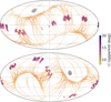 |
Fig. 1 Top: right ascension and declination map distribution of the Gaia targets possessing a Gaia rotation period from DR2 or DR3 and an EVEREST K2 light curve. The magnitude G is colour-coded. The full sample of Gaia targets with a rotation period in DR3 is shown for reference (Distefano et al. 2023) with their density colour-coded in orange. The location of the Kepler field is shown in grey. Bottom: same for the galactic location of the targets. |
3 Results
3.1 Rotation period in K2 versus Gaia
Among the sample of 1063 stars we analysed, we were able to extract 598 periods lying between 0.45 and 2.1 times the Gaia value and achieving a ROOSTER rotation score above 0.5. These validation criteria were deliberately relaxed. In particular, we wanted to account for the fact that most of the observations were not contemporaneous, meaning that the observable rotation periods may show significant variations due to the latitudinal migration of active regions with time. Hereafter we refer to this sample as the cross-validated sample. For 146 more stars, the K2 rotation period is outside of the range defined above, but the ROOSTER rotation score is above 0.9, supporting a reliable detection of rotation. As there is no independent validation of the K2 measurement from the Gaia observations for these stars, we required a higher ROOSTER score in order to keep these stars in our sample. We discuss the properties of these stars further in Sect. 4.1. Among this sample of 744 stars, 522 have reference Gaia measurements from DR3 and we use the values from Gaia DR2 for the 222 other stars. Their properties are summarised in Table D.1. For the 319 remaining stars, a visual inspection of their light curves and the results of the rotational analysis confirmed that the quality of the K2 observations was not sufficient to extract any useful observables for these targets. We therefore do not consider these remaining stars in what follows. In addition, unless mentioned otherwise, the Prot we display for the stars in our sample is the value obtained from the K2 light curves. In order to further validate the reliability of our K2 measurements, we compared our results with those obtained by Reinhold & Hekker (2020). Among our 744 stars, they published a rotation measurement for 337 targets, for which we obtain a very good agreement, beyond 95% (see Appendix C).
In Fig. 3, we compare the location of the stars in this sample in the diagram GBP - GRP versus apparent G magnitude to the Gaia DR3 stars with rotation periods and to the Kepler sample from Santos et al. (2019, 2021). The faint star cutoff is clearly visible in the Kepler stars as the distribution density abruptly decreases beyond G = 16. This cutoff is also visible in our K2 sample; we note that most of the targets beyond it are M-type stars, consistently with the fact that Gaia is able to probe a population of stars much more distant and fainter than the bulk population included in the Kepler Input Catalog (KIC) and the EPIC. We used the GBP - GRP measurements from Gaia DR3, which are available for the entirety of our sample, except for four targets. As the measurements from Gaia DR2 and DR3 are not homogeneous, these four stars are not displayed in the figures.
For this figure and all that follow, when possible we corrected the GBP - GRP value by subtracting the dereddening coefficient computed by the Gaia astrophysical parameter inference system (Apsis, Bailer-Jones et al. 2013; Creevey et al. 2023; Fouesneau et al. 2023).
The magnitude cutoff also has an impact when considering the absolute magnitude MG computed by the Apsis, as shown in Fig. 4. The MG distribution of our sample is very similar to the Kepler distribution, except for the group of brighter stars visible in the upper left corner. We recall that Santos et al. (2021) considered subgiant stars that are not considered in the Gaia rotation analysis. We also note that, at a given GBP - GRP colour, the MG range is wider for the Gaia population than for the stars observed by Kepler/K2, including significantly more stars that are less bright for a given GBP - GRP colour.
In Fig. 5, we show the GBP - GRP versus Prot diagram for our sample, compared with the reference distributions of Kepler and Gaia DR3 targets. This diagram is useful in order to characterise the rotational regime in which the K2-Gaia cross-match stars are located. The Gaia survey is shifted towards short periods with comparison to the Kepler measurements. The short-period cutoff of ∼0.3 days used for Gaia is visible. We also note that the bi-modality of the Kepler distribution (McQuillan et al. 2014), also detected in K2 (Gordon et al. 2021) is not apparent in Gaia, probably because the feature is blurred by the reduced precision of Gaia measurements in this range of periods. Most of the F- and G-type stars from the K2 sample occupy a region in the GBP - GRP versus Prot parameter space that corresponds to the young and fast rotators observed in Kepler for these given spectral types. This population corresponds to the first of the two groups of rotators characterised by Gaia for these spectral types, the second being composed of much faster rotators. For the second type, a comparison of the K2 periods with the Kepler distribution shows that most of the K- and M-type stars from the sample have not converged yet on the slow-rotator gyrochronological sequence. As expected, the Sph values are strongly anti-correlated with Prot, increasing as Prot decreases.
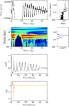 |
Fig. 2 From top to bottom: light curve (left) and power spectral density (right), WPS (left) and GWPS (right), ACF, and CS for EPIC 201121691. The set of Gaussian profiles fitted on the GWPS and the CS are shown in blue and orange, respectively. |
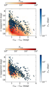 |
Fig. 3 Apparent magnitude G vs GBP - GRP diagram. Prot is colour-coded for the stars where the rotation period measured between K2 and Gaia is cross-validated. In the top panel the density distribution of stars with a Gaia rotation period is shown, while in the bottom panel our sample is compared to the distribution of the Kepler stars for which Santos et al. (2019, 2021) provided a rotation period. |
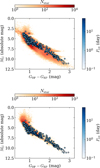 |
Fig. 4 Absolute magnitude MG vs GBP - GRP diagram. Prot is colour-coded for the stars where the rotation period measured between K2 and Gaia is cross-validated. In the top panel the density distribution of stars with a Gaia rotation period is shown, while in the bottom panel our sample is compared to the distribution of the Kepler stars for which Santos et al. (2019, 2021) provided a rotation period. |
3.2 Photometric activity index comparison
The K2 and Gaia rotation measurements allow us to derive photometric activity proxies. The K2 activity proxy that we use in this work is the Sph defined in Sect. 2.2 and already shown in the GBP - GRP versus Prot plot from Fig. 5. For a Gaia star with n observed segments, the Gaia activity proxy in the G band is defined as
![Mathematical equation: A_{\rm max} [G] = \max\limits_{i \in n} (G_{95\mathrm{th}, i} - G_{5\mathrm{th}, i}) ,](/articles/aa/full_html/2025/09/aa53912-25/aa53912-25-eq1.png) (1)
(1)
where G95th,i and G5th,i are the 95th and the 5th percentile of the G magnitude distribution in the ith segment.
We can see in Fig. 6 that most of the stars in our sample are located on the active edge of the Kepler distribution, while on the contrary Fig. 7 shows that they sample uniformly the Gaia distribution, with the notable exception of the region where the Gaia low-activity UFR stars are concentrated (see Lanzafame et al. 2019), and the upper right edge (slow and active rotators), which are also depleted. The absence of low-activity UFR stars in K2 can be explained considering the relationship between the apparent magnitude G and Amax[G]. As G increases, the rotation modulation detection of small amplitudes becomes more difficult with K2, as illustrated in Fig. 10. When we compare the Amax[G] versus G distribution of the K2 sample with the Gaia DR3 low-activity UFR sample, selected using the criterion defined by Lanzafame et al. (2019), i.e. Prot < 0.5 and Amax[G] < 0.05. Considering stars located at and absolute ecliptic latitude lower than 10° (which is roughly the range of latitude explored by the K2 mission), we see that there is almost no overlap between the two populations. Only nine stars in our cross-validated sample are inside the area defined by the Lanzafame et al. (2019) criterion, and most of them are on the high-activity edge of the UFR distribution (see Fig. 7). For the rest, we note that most of the K2 stars that are located close to the bulk area of the UFR in the Amax[G] versus G diagram are not fast rotators. This suggests that the UFR corresponds to a population of stars that is located further away from us than the objects observed by Kepler and K2.
It should also be noted that, given the selection cutoff operated for Gaia, the post-Kraft break F-type stars with fast rotation and low activity, visible in the lower left part of Fig. 6 (see Santos et al. 2021), are not represented in our sample, as already noted by Distefano et al. (2023). The correlation between Sph and Amax[G] is already apparent in these two diagrams.
In Fig. 8, we directly compare the Sph index to Amax[G]. Considering the Pearson correlation coefficients p4 between G magnitude variation and GBP - GRP colour provided segment-wise in the Gaia rotation catalogue, we also compute a mean correlation coefficient ρ̄ that we show together with the two activity indexes. Unavailable from mono-band photometric observations such as those performed by Kepler/K2, this coefficient therefore quantifies the level of correlation between the variation of the stellar apparent magnitude and the stellar colour. In other words, a positive coefficient means that an apparent darkening of the star (e.g. when star spots appear in the field of view) goes with a reddening of its emitted spectrum, while a star with a negative coefficient becomes bluer when darkening. The correlation case can be schematically interpreted as the passage of a cold dark spot which results in a simultaneous darkening and reddening of the stellar disc. A strong anti-correlation suggests on the contrary that the modulation is connected to the orbit of a hotter eclipsing companion. The ρ̄ coefficient is positive for the vast majority of the stars; only a few of them exhibit an anti-correlated behaviour. An important property that we highlight is that ρ̄ tends to increase with Sph index and Amax[G], as visible in Fig. 9, where we directly compare Sph and Amax[G] with ρ̄. Interestingly, for a small fraction of active stars, we have p < 0.
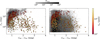 |
Fig. 5 Prot vs GBP - GRP diagram. The Sph value is colour-coded for the stars for which the Gaia and K2 rotation measurements are cross-validated. In the left panel, the sample is compared with the density distribution of the Kepler stars from Santos et al. (2019, 2021, in grey) while in the right panel it is compared with the density distribution of the stars from Gaia DR3 (in grey). |
 |
Fig. 6 S ph vs Prot diagram for the stars where the rotation period measured between K2 and Gaia is cross-validated. The Gaia activity index Amax[G] is colour-coded. The Kepler distribution from Santos et al. (2019, 2021) is shown in grey for comparison. The median value of the binned distribution along Prot is shown in blue. |
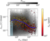 |
Fig. 7 Amax[G] vs Prot diagram for the stars where the rotation period measured between K2 and Gaia is cross-validated. The Sph is colour-coded. The full Gaia DR3 distribution from Distefano et al. (2023) is shown in grey for comparison. The median value of the binned distribution along Prot is shown in blue. The hatched blue area correspond to the UFR criterion selection from Lanzafame et al. (2019). |
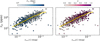 |
Fig. 8 Sph vs Amax [G] diagram for the stars where the rotation period measured between K2 and Gaia is cross-validated. In the left panel Prot are colour-coded, while in the right panel the mean Pearson correlation coefficient ρ̄ is colour-coded. For readability, ρ̄ values are colour-coded only in the 0 to 1 range. In both panels, the median value of the binned distribution along Amax [G] is shown in blue. |
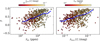 |
Fig. 9 Left: ρ̄ vs S ph diagram for the stars where the rotation period measured between K2 and Gaia is cross-validated. Amax[G] is colour-coded. The median value of the binned distribution along Amax[G] is shown in blue. Right: ρ̄ vs Amax[G] diagram for the stars where the rotation period measured between K2 and Gaia is cross-validated. Sph is colour-coded. The median value of the binned distribution along Sph is shown in blue. |
3.3 Targets with Gaia spectroscopic characterisation
In this section, we now consider all the stars of our sample for which we were able to measure a reliable rotation period from the K2 EVEREST light curve, and we turn to the possibilities of characterisation offered by Gaia infrared spectroscopic observations. Using the RVS data, Lanzafame et al. (2023) derived a chromospheric activity index αCaII-IRT. The αCaII-IRT being relevant only to compare stars with similar global properties, Lanzafame et al. (2023) defined the R′IRT activity indicator and provided the following formula to estimate it from the effective temperature, Teff, the metallicity, [M/H], and αCaII-IRT:
 (2)
(2)
Here θ = log Teff, and the logarithms are decimal logarithms. The ci coefficients depend on [M/H] and are interpolated using Table 1 from Lanzafame et al. (2023). Given the bounds of this table, we computed log R′IRT only for stars within the range −0.5 < [M/H] < 0.5. We also removed stars for which αCaII-IRT is smaller than three times its uncertainties, as the αCaII-IRT measurement in this case is probably dominated by random noise, and those who have log R′IRT < −5.7, as these stars can be considered inactive. To obtain a homogeneous sample, we considered only stars for which a Gaia RVS spectroscopic Teff and [M/H] values are available.
We directly compare log R′IRT to Sph and Amax[G] in Figs. 11 and 12, respectively. Although Sph and Amax[G] are both correlated with log R′IRT, there is a strong dispersion in the relation between the parameters. We recall that photometric activity indicators such as Sph and Amax[G] are only lower-limit proxies of activity as they might be biased by the inclination of the stellar rotation axis with respect to the observer’s line of sight, as well as the latitude of emergence of the active regions. We also verified again that the stars in our sample coincide with the active edge (larger log R′IRT) of the Kepler distribution.
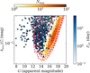 |
Fig. 10 Amax [G] vs G diagram for K2 stars (dots) with Prot colour-coded, compared with the density map of Gaia DR3 low-activity UFR stars located at absolute ecliptic latitude lower than 10°. The density contours (dashed red) of the full Gaia DR3 rotation catalogue are represented for comparison. |
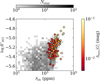 |
Fig. 11 log R′IRT vs Sph diagram with Amax[G] colour-coded for all stars with a reliable K2 rotation measurement where log R′IRT could be computed. The distribution of Kepler stars from Santos et al. (2019, 2021) for which log R′IRT could be computed is shown for comparison. |
4 Discussion
4.1 Discrepancies between Gaia and K2
As stated in Sect. 3.1, while we found consistent measurements for more than 80% of the stars where we validate the rotation measurements in the K2 light curve, the rotation periods obtained from the Gaia observations and K2 light curves differ for a fraction of this sample.
Before exploring in greater depth the origins of these differences, it is interesting to summarise and briefly discuss the respective advantages of Gaia and Kepler/K2 when it comes to measuring stellar surface rotation. On the one hand, the Kepler/K2 standard cadence of 30 minutes is well suited for surface activity modulation follow-up, but while most Kepler targets have a four-year light curve, the design of the K2 mission has uses K2 light curves that are 90-day segments, which in turn limits the possibility to monitor rotation in slow rotators. On the other hand, the Gaia observations are sparse but cover several years; the high photometric precision of the observation makes them ideal to monitor the long-term activity-induced modulation of the observed stars. In addition, the Gaia pixel size is several orders of magnitude smaller (59 milliarcsecond in the scanning direction) than for Kepler (3.98 arcsecond per pixel), which is important in the case of crowded fields, where light curves can be contaminated by neighbouring stars of similar brightness. The Gaia sensitivity also allows it to observe fainter stars (as already mentioned in Sect. 3.1 and Fig. 3), and it has access to multicolour photometry, while Kepler/K2 is mono-band. Finally, we note that the high cadence of Kepler/K2 is necessary in order to perform more in-depth studies of the morphology of the active regions (e.g. starspot modelling, see Lanza 2016; Breton et al. 2024a).
We recall that the rotation periods were measured in Gaia using the following methodology (Lanzafame et al. 2018; Distefano et al. 2023). For a given star, in each time series segment obtained by the instrument, the highest peak of the Lomb-Scargle periodogram (Lomb 1976; Scargle 1982; Zechmeister & Kürster 2009) is selected and validated if its false alarm probability is below 0.05. In this case, a sinusoidal model is fitted on the data in order to estimate the amplitude of the modulation. Finally, considering the set of periods extracted from the different segment, the mode of the distribution is taken as the best rotation period (see Lanzafame et al. 2018, for more details). Each segment contains at least 12 Gaia measurements and lasts no longer than 120 days (Lanzafame et al. 2018).
In order to investigate the possible origins of these discrepancies, we compare in Fig. 13 the rotation periods we extracted from the K2 light curves to the reference Gaia periods from DR2 and DR3. On the one hand, the diagram shows that, up to Prot ∼ 3–4 days, the overall agreement between K2 and Gaia is very good, validating that Gaia is extremely efficient at recovering rotation periods for fast rotators. On the other hand, for inconsistent measurements, we note that Gaia tends to underestimate the stellar rotation period in the majority of the cases, although in some cases the Gaia rotation period is overestimated.
It is important to note that stars outside the cross-validated sample exhibit in general a small activity index Amax[G] and a small correlation coefficient ρ̄. We also consider the stability criterion defined by Distefano et al. (2023): a star is flagged as having a stable modulation if the Gaia best rotation period differs by less than 5% from the main periodicity in the full Gaia time series. We note that 57% of the stars in the crossvalidated sample fulfil this stability criterion, while it is the case of only 47% of the other sample. This suggest that these different parameters may be used as quality assessments quantities. Another aspect to keep in mind is that the K2 stars we deal with have been observed by Gaia in a maximum of six segments. At different ecliptic latitudes, especially around 45° and close to the ecliptic pole, stars have been observed during a significantly larger number of visits (see Distefano et al. 2023). We also compare in Fig. 14 the location of the two populations on the Prot versus GBP - GRP diagram, with the inferred Sph as colourcoding. Again, in this diagram, we see that the distribution of the two subsamples is quite different: the stars with inconsistent measurements are concentrated on the bulk of the Kepler distribution.
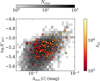 |
Fig. 12 log R′IRT vs Amax[G] diagram with Sph colour-coded for all stars with a reliable K2 rotation measurement where log R′IRT could be computed. The distribution of Gaia DR3 stars with rotation measurements for which log R′IRT could be computed is shown for comparison. |
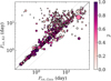 |
Fig. 13 Comparison between the rotation periods measured and validated in the K2 light curves, Prot,K2, and the reference values from the Gaia DR2 and DR3 catalogues, Prot,Gaia. The 1:0.45, 1:2.1 (dotted grey lines), and 1:1 (dashed black line) lines are shown. The mean correlation coefficient ρ̄ is colour-coded, and the dot size is proportional to the Amax[G] index. For readability, the ρ̄ values are colour-coded only in the 0 to 1 range. |
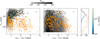 |
Fig. 14 Prot vs GBP - GRP diagram. The Sph value is colour-coded for the stars for which Gaia and K2 rotation measurements are cross-validated. The stars for which the measurements are consistent are shown in orange. In the left panel the sample is compared with the density distribution of the Kepler stars from Santos et al. (2019, 2021) (in grey), while in the right panel it is compared with the density distribution of the stars from Gaia DR3 (in grey). |
4.2 Identifying Gaia stars similar to the K2 subsample
In this section, we investigate the possibility of selecting Gaia stars that have properties similar to those in the K2 crossvalidated sample. To do so, we used the local outlier factor (LOF, Breunig et al. 2000), with the implementation provided by scikit-learn (Pedregosa et al. 2011). The LOF is an unsupervised method that is able to measure the local density of element clusters in a dataset and, from this, to estimate the degree of abnormality of unknown elements. A data point with a LOF close to 1 can be interpreted as a probable inlier, while a higher value suggests that the element is an outlier. It should be noted that there is no strict threshold distinguishing inliers from outliers and that the cutoff choice to separate inliers from outliers is therefore arbitrary. It is also important to keep in mind that the method allows the LOF of each element of the training dataset to be obtained, and that these LOFs are not mandatorily close to 1, depending on the position of a given element with respect to the density distribution of the dataset.
The parameters we used to compute the LOFs are the following: Gaia rotation period and corresponding error, Amax[G] activity index, number of observed segments, mean correlation coefficient, periodicity stability criterion, higher and lower value of the Lomb–Scargle false alarm probability estimated for the observation segments, magnitude G, and GBP - GRP. In Fig. 15 we compare the LOF distribution obtained for the reference K2 cross-validated sample and the LOF distribution of the other stars in the Gaia DR3 rotation catalogue. We note that while most of the stars in the reference sample have a LOF close to 1, there exist a tail of elements with a higher LOF, and therefore a higher degree of abnormality in the cross-validated sample. Additionally, only a small fraction of the Gaia DR3 rotation catalogue targets have a LOF close to 1. Selecting only stars with LOF ≤ 1.1 (i.e. 40 423 objects), we represent them in the Amax [G] versus Prot,Gaia plot in Fig. 16. Although some of the selected stars are fast rotators with a low level of activity (some of them laying in the UFR region), and very few stars with Prot > 20 days have been selected, we note that the parameter space covered by the stars with LOF ≤ 1.1 is globally located close to the bulk of the cross-validated K2 sample. As these values should be useful for future statistical studies, the full set of computed LOFs is available and is summarised in Table 1.
Excerpt of the table summarising the properties of the stars in the Gaia DR3 catalogue and their LOFs.
 |
Fig. 15 LOF computed for our K2 subsample (orange) and for the full set of Gaia DR3 stars (blue). |
5 Conclusion
In this work, we combined Gaia and K2 observations to characterise the sample of rotating solar-type stars that were observed by both missions. The rotation periods we extracted from the EVEREST reduction of the K2 observations were globally in good agreement with the Gaia measurements, especially for the fast rotators (Prot below 3–4 days). We discussed the discrepancies we observed between Gaia and K2 for a fraction of our sample, noting that these stars were slow rotators with a low level of activity, for which photometric rotation measurements are notoriously difficult to carry out. We also recalled the limited number of segments available for Gaia at the ecliptic latitudes where K2 stars are located. We also noted that the Gaia low-activity UFR population discussed by Lanzafame et al. (2019) is not represented in our K2 sample, preventing us from investigating the properties of this region of the diagram. In the context of this work, the elusive character of the UFR is explained by the fact that their Amax[G] versus G relationship makes the vast majority of them inaccessible for the instrumental capabilities of K2 (see Fig. 10). We proceeded to an extensive comparison of the photometric activity indicators obtained by each missions. We then considered the cases of the targets for which Gaia RVS observations are available, which allowed us to run a comparison between the log R′IRT indicator defined by Lanzafame et al. (2023) and the Sph photometric indicator, for both Kepler and K2 stars. Finally, noting that in our sample the stars with consistent K2 and Gaia parameters exhibit distinct properties in term of variability amplitude and correlation between the different Gaia colours, we computed the LOF of every star in the Gaia DR3 rotation catalogues with the K2 cross-validated sample as reference. We showed that the rotation–activity distribution of the 40 423 stars with LOF ≤ 1.1 exhibited a good similarity to the cross-validated K2 sample, which make them a good subsample to consider for future statistical studies.
Concerning other space missions, we anticipate that, due to their common strategy of full-scale coverage, TESS and Gaia should have an important number of stars with measured rotation in common. However, we recall that the 27-day sector length of the TESS observations means that it is difficult to measure the rotation periods of moderately slow and slow rotators located outside of the TESS continuous viewing zone. In this sense, the possibility to work with long temporal baseline continuous observations such as those that will be acquired by PLATO is crucial. The intersection between the two long-pointing PLATO fields of observation and Gaia targets with measured rotation periods should remain limited (see Fig. 2 from Nascimbeni et al. 2022, compared to our Fig. 1), but a fraction of the PLATO stars should still possess previous Gaia rotation measurements. Nevertheless, future data releases from Gaia should provide an increased set of activity indicators and rotation measurements for stars in the PLATO fields.
 |
Fig. 16 Amax[G] vs Prot,Gaia diagram for Gaia DR3 stars which have a LOF ≤ 1.1. The density of stars is colour-coded. The K2 cross-validated sample is shown in orange for comparison. |
Acknowledgements
The authors want to thank the anonymous referee for helpful comments that allowed improving the manuscript. S.N.B. acknowledges support from PLATO ASI-INAF agreement no. 2022-28-HH.0 “PLATO Fase D”. D.B.P. acknowledges support from PLATO CNES grant. S.N.B. thanks A.F. Lanza and R.A. García for useful discussions and advices. This paper includes data collected by the Kepler mission and obtained from the MAST data archive at the Space Telescope Science Institute (STScI). Funding for the Kepler mission is provided by the NASA Science Mission Directorate. STScI is operated by the Association of Universities for Research in Astronomy, Inc., under NASA contract NAS 5–26555. This work has made use of data from the European Space Agency (ESA) mission Gaia (https://www.cosmos.esa.int/gaia), processed by the Gaia Data Processing and Analysis Consortium (DPAC, https://www.cosmos.esa.int/web/gaia/dpac/consortium). Funding for the DPAC has been provided by national institutions, in particular the institutions participating in the Gaia Multilateral Agreement. This work made use of the gaia-kepler.fun crossmatch database created by Megan Bedell. This research made use of Lightkurve, a Python package for Kepler and TESS data analysis. Software: star-privateer (Breton et al. 2024b), numpy (Harris et al. 2020), matplotlib (Hunter 2007), scipy (Virtanen et al. 2020), astropy (Astropy Collaboration 2022), astroquery (Ginsburg et al. 2019), pandas (The pandas development team 2020), lightkurve (Lightkurve Collaboration 2018), scikit-learn (Pedregosa et al. 2011).
Data availability
Tables 1 and D.1 are available at the CDS via https://cdsarc.cds.unistra.fr/viz-bin/cat/J/A+A/701/A263.
Appendix A Targets belonging to open clusters
By cross-matching our list of targets with the cluster membership catalogue from Hunt & Reffert (2023), we find that 78 stars for which we were able to measure a rotation periods are part of known open clusters with a probability larger than 0.5. Among these stars, 28 belong to Pleiades, 25 to Praesepe, and 9 to Hyades. Rebull et al. (2016a,b); Stauffer et al. (2016) used K2 light curves to perform an extensive study of stellar variability in about one thousand candidate Pleiades members, reporting rotation measurements for 716 high-confidence members of the cluster. Brown et al. (2021) showed that stars for Pleiades exhibited the mid-frequency continuum (MFC), a signal of probable magnetic origin that significantly contributed to the variability of the targets where it was found, without being correlated with the modulation amplitude from active regions. Rotational properties in Praesepe were also already explored with K2 by Douglas et al. (2017), who reported rotation measurements for 677 targets. More recently, rotation periods for stars in Pleiades, Praesepe, and Hyades were provided by Long et al. (2023), among other open clusters. The age of Hyades is between 500 and 800 Myr (Pérez-Garrido et al. 2018), while for the Praesepe cluster it is thought to be between 580 and 700 Myr (Gossage et al. 2018; Douglas et al. 2019). We show in Fig. A.1 to the GBP -GRP versus Prot,K2 diagram. Praesepe and Hyades stars are globally slower rotators as expected from the age difference with Pleiades. The Prot,K2 versus Ssph diagram of Fig. A.2 shows that the slowest rotators of Praesepe and Hyades have transitioned towards less active regimes, while some of them still have an activity level comparable with the one observed in Pleiades.
 |
Fig. A.1 Prot vs GBP - GRP diagram for Praesepe (red), Pleiades (blue), and NGC 1647 (yellow) stars. The other stars in our sample are represented in grey for comparison. |
 |
Fig. A.2 Sph vs Prot diagram for Praesepe (red), Pleiades (blue), and NGC 1647 (yellow) stars. The other stars in our sample are represented in grey for comparison. |
Appendix B ROOSTER training set
In this Appendix we describe how the ROOSTER training set was adapted in order to correctly predict the rotation periods of the K2 targets. The training set for this work is composed of Kepler stars with rotation measurements performed by Santos et al. (2019, 2021). We consider the KEPSEISMIC light curves (García et al. 2011, 2014; Pires et al. 2015) where the signal beyond 55 day has been filtered out. Given the length of the K2 light curves and the prior knowledge on the period distribution provided by Gaia, we expect to have a significant number of fast rotators in the sample. We therefore included in the training set a first sample of 996 targets that includes all Kepler stars with periods below 1 day and a random selection of Kepler stars with periods spanning from 1 to 15 days. We then completed the sample with 996 more stars with no prior selection on the rotation periods, and 995 for which Santos et al. (2019, 2021) were not able to perform a measurement of the rotation period. This makes a total of 2987 stars in the training set.
Kepler light curves are four years long, spanning from 2009 to 2013, while K2 light curves are significantly shorter (about 90 days). In order to ensure that ROOSTER was trained with a set of parameters comparable to the ones we extracted from the K2 light curves, we subdivided our Kepler light curves in 90-day long chunks, and decided to consider each of these chunks independently. We then computed the GWPS, ACF, and CS of each of these chunks as outlined in Sect. 2.2.
The training parameters we considered are the following: the candidate rotation periods obtained with each methods, the width of the corresponding Gaussian profiles fitted in the case of the GWPS and CS (which are used as uncertainties on the period), the Sph value computed from each candidate period, its corresponding error, the HACF and GACF control parameters (Breton et al. 2021, e.g.), and the summary parameters of the Gaussian profiles fitted in the GWPS and CS (amplitude, central period, width, uncertainty).
For stars with measured rotation periods, we use a given 90-day chunk in the training set only if one of the candidate rotation periods match the reference values with a 10 % tolerance, otherwise we remove the chunk from the training sample. ROOSTER is finally trained with 16686 light curve chunks of stars with detected rotation and 10693 light curve chunks of stars without detection. It is tested with 4187 light curve chunks of stars with detected rotation and 2674 light curve chunks of stars without detection.
Appendix C Comparison with Reinhold & Hekker (2020)
Some of the stars for which we measured rotation in this work are part of the catalogue published by Reinhold & Hekker (2020)5. Over our 744 stars with measured rotation periods, we found 337 stars in common. As, for each star, Reinhold & Hekker (2020) provided one value per campaign of observation, when dealing with stars with multiple measurements, we considered only the closest value to our own measurement. As it is possible to see it in Fig. C.1, the agreement is very good: out of the 337 stars, 326 measurements are compatible within 25%. The majority of the stars outside this region (9 stars over 11) are close to the 1:2 and 1:0.5 line, suggesting a possible confusion between the fundamental period and its first overtone.
 |
Fig. C.1 Comparison between our measurements, Prot;ROOSTER, and those from Reinhold & Hekker (2020), Prot,K2;RH2020. The top panel shows Prot,K2;RoosTER vs Prot,K2;RH2020, while the bottom panel shows ΔProt,K2 vs Prot,K2;RH2020 with ΔProt,K2 = (Prot,K2;ROOSTER - Prot,K2;RH2020)/Prot,K2;RH2020. The 1:0.5, 1:2 (dotted grey lines), 1:0.75, 1:1.25 (dotted black lines), and 1:1 (dashed black line) lines are shown. |
Appendix D Summary table
Table D.1 summarises the properties of the 744 targets for which we measured a rotation period in the K2 light curve.
Excerpt of the table summarising the properties of the K2 stars studied in this work.
References
- Aigrain, S., Llama, J., Ceillier, T., et al. 2015, MNRAS, 450, 3211 [Google Scholar]
- Astropy Collaboration (Price-Whelan, A. M., et al.) 2022, ApJ, 935, 167 [NASA ADS] [CrossRef] [Google Scholar]
- Bailer-Jones, C. A. L., Andrae, R., Arcay, B., et al. 2013, A&A, 559, A74 [NASA ADS] [CrossRef] [EDP Sciences] [Google Scholar]
- Barnes, S. A. 2003, ApJ, 586, 464 [Google Scholar]
- Barnes, S. A. 2007, ApJ, 669, 1167 [Google Scholar]
- Borucki, W. J., Koch, D., Basri, G., et al. 2010, Science, 327, 977 [Google Scholar]
- Breton, S. N., Santos, A. R. G., Bugnet, L., et al. 2021, A&A, 647, A125 [EDP Sciences] [Google Scholar]
- Breton, S. N., Lanza, A. F., & Messina, S. 2024a, A&A, 682, A67 [NASA ADS] [CrossRef] [EDP Sciences] [Google Scholar]
- Breton, S. N., Lanza, A. F., Messina, S., et al. 2024b, A&A, 689, A229 [NASA ADS] [CrossRef] [EDP Sciences] [Google Scholar]
- Breunig, M. M., Kriegel, H.-P., Ng, R. T., & Sander, J. 2000, SIGMOD Rec., 29, 93 [Google Scholar]
- Brown, T. M., García, R. A., Mathur, S., Metcalfe, T. S., & Santos, Â. R. G. 2021, ApJ, 916, 66 [Google Scholar]
- Brun, A. S., & Browning, M. K. 2017, Living Rev. Solar Phys., 14, 4 [Google Scholar]
- Ceillier, T., Tayar, J., Mathur, S., et al. 2017, A&A, 605, A111 [NASA ADS] [CrossRef] [EDP Sciences] [Google Scholar]
- Creevey, O. L., Sordo, R., Pailler, F., et al. 2023, A&A, 674, A26 [NASA ADS] [CrossRef] [EDP Sciences] [Google Scholar]
- Distefano, E., Lanzafame, A. C., Brugaletta, E., et al. 2023, A&A, 674, A20 [NASA ADS] [CrossRef] [EDP Sciences] [Google Scholar]
- Douglas, S. T., Agüeros, M. A., Covey, K. R., & Kraus, A. 2017, ApJ, 842, 83 [Google Scholar]
- Douglas, S. T., Curtis, J. L., Agüeros, M. A., et al. 2019, ApJ, 879, 100 [Google Scholar]
- Fouesneau, M., Frémat, Y., Andrae, R., et al. 2023, A&A, 674, A28 [NASA ADS] [CrossRef] [EDP Sciences] [Google Scholar]
- Gaia Collaboration (Prusti, T., et al.) 2016, A&A, 595, A1 [NASA ADS] [CrossRef] [EDP Sciences] [Google Scholar]
- Gaia Collaboration (Brown, A. G. A., et al.) 2018, A&A, 616, A1 [NASA ADS] [CrossRef] [EDP Sciences] [Google Scholar]
- Gaia Collaboration (Brown, A. G. A., et al.) 2021, A&A, 649, A1 [NASA ADS] [CrossRef] [EDP Sciences] [Google Scholar]
- Gaia Collaboration (Vallenari, A., et al.) 2023, A&A, 674, A1 [NASA ADS] [CrossRef] [EDP Sciences] [Google Scholar]
- García, R. A., Hekker, S., Stello, D., et al. 2011, MNRAS, 414, L6 [NASA ADS] [CrossRef] [Google Scholar]
- García, R. A., Mathur, S., Pires, S., et al. 2014, A&A, 568, A10 [Google Scholar]
- Ginsburg, A., Sipo˝cz, B. M., Brasseur, C. E., et al. 2019, AJ, 157, 98 [NASA ADS] [CrossRef] [Google Scholar]
- Gordon, T. A., Davenport, J. R. A., Angus, R., et al. 2021, ApJ, 913, 70 [Google Scholar]
- Gossage, S., Conroy, C., Dotter, A., et al. 2018, ApJ, 863, 67 [Google Scholar]
- Hall, O. J., Davies, G. R., van Saders, J., et al. 2021, Nat. Astron., 5, 707 [NASA ADS] [CrossRef] [Google Scholar]
- Harris, C. R., Millman, K. J., van der Walt, S. J., et al. 2020, Nature, 585, 357 [NASA ADS] [CrossRef] [Google Scholar]
- Howell, S. B., Sobeck, C., Haas, M., et al. 2014, PASP, 126, 398 [Google Scholar]
- Hunt, E. L., & Reffert, S. 2023, A&A, 673, A114 [NASA ADS] [CrossRef] [EDP Sciences] [Google Scholar]
- Hunter, J. D. 2007, Comput. Sci. Eng., 9, 90 [NASA ADS] [CrossRef] [Google Scholar]
- Lanza, A. F. 2016, in Lecture Notes in Physics, 914, eds. J.-P. Rozelot, & C. Neiner (Berlin: Springer Verlag), 43 [Google Scholar]
- Lanzafame, A. C., & Spada, F. 2015, A&A, 584, A30 [NASA ADS] [CrossRef] [EDP Sciences] [Google Scholar]
- Lanzafame, A. C., Distefano, E., Messina, S., et al. 2018, A&A, 616, A16 [NASA ADS] [CrossRef] [EDP Sciences] [Google Scholar]
- Lanzafame, A. C., Distefano, E., Barnes, S. A., & Spada, F. 2019, ApJ, 877, 157 [NASA ADS] [CrossRef] [Google Scholar]
- Lanzafame, A. C., Brugaletta, E., Frémat, Y., et al. 2023, A&A, 674, A30 [NASA ADS] [CrossRef] [EDP Sciences] [Google Scholar]
- Lightkurve Collaboration (Cardoso, J. V. d. M., et al.) 2018, Astrophysics Source Code Library [record ascl:1812.013] [Google Scholar]
- Liu, Y., San Liang, X., & Weisberg, R. H. 2007, J. Atmos. Oceanic Technol., 24, 2093 [Google Scholar]
- Lomb, N. R. 1976, Ap&SS, 39, 447 [Google Scholar]
- Long, L., Bi, S., Zhang, J., et al. 2023, ApJS, 268, 30 [Google Scholar]
- Lu, Y. L., Curtis, J. L., Angus, R., David, T. J., & Hattori, S. 2022, AJ, 164, 251 [CrossRef] [Google Scholar]
- Luger, R., Agol, E., Kruse, E., et al. 2016, AJ, 152, 100 [Google Scholar]
- Mathur, S., García, R. A., Régulo, C., et al. 2010, A&A, 511, A46 [NASA ADS] [CrossRef] [EDP Sciences] [Google Scholar]
- Mathur, S., García, R. A., Ballot, J., et al. 2014a, A&A, 562, A124 [NASA ADS] [CrossRef] [EDP Sciences] [Google Scholar]
- Mathur, S., Salabert, D., García, R. A., & Ceillier, T. 2014b, J. Space Weather Space Climate, 4, A15 [NASA ADS] [CrossRef] [EDP Sciences] [Google Scholar]
- McQuillan, A., Aigrain, S., & Mazeh, T. 2013, MNRAS, 432, 1203 [Google Scholar]
- Mathur, S., Claytor, Z. R., Santos, Â. R. G., et al. 2023, ApJ, 952, 131 [NASA ADS] [CrossRef] [Google Scholar]
- McQuillan, A., Mazeh, T., & Aigrain, S. 2014, ApJS, 211, 24 [Google Scholar]
- Metcalfe, T. S., Finley, A. J., Kochukhov, O., et al. 2022, ApJ, 933, L17 [NASA ADS] [CrossRef] [Google Scholar]
- Moreno, J., Buttry, R., O’Brien, J., et al. 2021, AJ, 162, 232 [Google Scholar]
- Nascimbeni, V., Piotto, G., Börner, A., et al. 2022, A&A, 658, A31 [NASA ADS] [CrossRef] [EDP Sciences] [Google Scholar]
- Pedregosa, F., Varoquaux, G., Gramfort, A., et al. 2011, J. Mach. Learn. Res., 12, 2825 [Google Scholar]
- Pérez-Garrido, A., Lodieu, N., Rebolo, R., & Chinchilla, P. 2018, A&A, 620, A130 [NASA ADS] [CrossRef] [EDP Sciences] [Google Scholar]
- Pires, S., Mathur, S., García, R. A., et al. 2015, A&A, 574, A18 [NASA ADS] [CrossRef] [EDP Sciences] [Google Scholar]
- Rauer, H., Aerts, C., Cabrera, J., et al. 2025, Exp. Astron., 59, 26 [Google Scholar]
- Rebull, L. M., Stauffer, J. R., Bouvier, J., et al. 2016a, AJ, 152, 113 [Google Scholar]
- Rebull, L. M., Stauffer, J. R., Bouvier, J., et al. 2016b, AJ, 152, 114 [NASA ADS] [CrossRef] [Google Scholar]
- Reinhold, T., & Hekker, S. 2020, A&A, 635, A43 [NASA ADS] [CrossRef] [EDP Sciences] [Google Scholar]
- Ricker, G. R., Winn, J. N., Vanderspek, R., et al. 2015, J. Astron. Telesc. Instrum. Syst., 1, 014003 [Google Scholar]
- Salabert, D., García, R. A., Jiménez, A., et al. 2017, A&A, 608, A87 [NASA ADS] [CrossRef] [EDP Sciences] [Google Scholar]
- Santos, A. R. G., García, R. A., Mathur, S., et al. 2019, ApJS, 244, 21 [Google Scholar]
- Santos, A. R. G., Breton, S. N., Mathur, S., & García, R. A. 2021, ApJS, 255, 17 [NASA ADS] [CrossRef] [Google Scholar]
- Santos, A. R. G., Godoy-Rivera, D., Finley, A. J., et al. 2024, Front. Astron. Space Sci., 11 [Google Scholar]
- Scargle, J. D. 1982, ApJ, 263, 835 [Google Scholar]
- Skumanich, A. 1972, ApJ, 171, 565 [Google Scholar]
- Spada, F., & Lanzafame, A. C. 2020, A&A, 636, A76 [NASA ADS] [CrossRef] [EDP Sciences] [Google Scholar]
- Stauffer, J., Rebull, L., Bouvier, J., et al. 2016, AJ, 152, 115 [Google Scholar]
- The pandas development team 2020, https://doi.org/10.5281/zenodo.3509134 [Google Scholar]
- Torrence, C., & Compo, G. P. 1998, Bull. Am. Meteorol. Soc., 79, 61 [Google Scholar]
- van Saders, J. L., Ceillier, T., Metcalfe, T. S., et al. 2016, Nature, 529, 181 [Google Scholar]
- Virtanen, P., Gommers, R., Oliphant, T. E., et al. 2020, Nat. Methods, 17, 261 [Google Scholar]
- Zechmeister, M., & Kürster, M. 2009, A&A, 496, 577 [CrossRef] [EDP Sciences] [Google Scholar]
The K2-Gaia DR2 cross-match is available here: https://gaia-kepler.fun
See the online documentation of the vari_rotation_modulation table: https://gea.esac.esa.int/archive/documentation/GDR3/Data_analysis/chap_cu7var/sec_cu7var_rotmod/
The source code is accessible at https://gitlab.com/sybreton/star_privateer and the corresponding documentation is hosted at https://star-privateer.readthedocs.io/en/latest
The activity index Amax[G] and the correlation coefficients ρ are provided in the Gaia database only for objects of the vari_rotation_modulation table.
The catalogue is accessible on Vizier: https://cdsarc.u-strasbg.fr/viz-bin/cat/J/A+A/635/A43
All Tables
Excerpt of the table summarising the properties of the stars in the Gaia DR3 catalogue and their LOFs.
Excerpt of the table summarising the properties of the K2 stars studied in this work.
All Figures
|
Fig. 1 Top: right ascension and declination map distribution of the Gaia targets possessing a Gaia rotation period from DR2 or DR3 and an EVEREST K2 light curve. The magnitude G is colour-coded. The full sample of Gaia targets with a rotation period in DR3 is shown for reference (Distefano et al. 2023) with their density colour-coded in orange. The location of the Kepler field is shown in grey. Bottom: same for the galactic location of the targets. |
| In the text | |
|
Fig. 2 From top to bottom: light curve (left) and power spectral density (right), WPS (left) and GWPS (right), ACF, and CS for EPIC 201121691. The set of Gaussian profiles fitted on the GWPS and the CS are shown in blue and orange, respectively. |
| In the text | |
|
Fig. 3 Apparent magnitude G vs GBP - GRP diagram. Prot is colour-coded for the stars where the rotation period measured between K2 and Gaia is cross-validated. In the top panel the density distribution of stars with a Gaia rotation period is shown, while in the bottom panel our sample is compared to the distribution of the Kepler stars for which Santos et al. (2019, 2021) provided a rotation period. |
| In the text | |
|
Fig. 4 Absolute magnitude MG vs GBP - GRP diagram. Prot is colour-coded for the stars where the rotation period measured between K2 and Gaia is cross-validated. In the top panel the density distribution of stars with a Gaia rotation period is shown, while in the bottom panel our sample is compared to the distribution of the Kepler stars for which Santos et al. (2019, 2021) provided a rotation period. |
| In the text | |
|
Fig. 5 Prot vs GBP - GRP diagram. The Sph value is colour-coded for the stars for which the Gaia and K2 rotation measurements are cross-validated. In the left panel, the sample is compared with the density distribution of the Kepler stars from Santos et al. (2019, 2021, in grey) while in the right panel it is compared with the density distribution of the stars from Gaia DR3 (in grey). |
| In the text | |
|
Fig. 6 S ph vs Prot diagram for the stars where the rotation period measured between K2 and Gaia is cross-validated. The Gaia activity index Amax[G] is colour-coded. The Kepler distribution from Santos et al. (2019, 2021) is shown in grey for comparison. The median value of the binned distribution along Prot is shown in blue. |
| In the text | |
|
Fig. 7 Amax[G] vs Prot diagram for the stars where the rotation period measured between K2 and Gaia is cross-validated. The Sph is colour-coded. The full Gaia DR3 distribution from Distefano et al. (2023) is shown in grey for comparison. The median value of the binned distribution along Prot is shown in blue. The hatched blue area correspond to the UFR criterion selection from Lanzafame et al. (2019). |
| In the text | |
|
Fig. 8 Sph vs Amax [G] diagram for the stars where the rotation period measured between K2 and Gaia is cross-validated. In the left panel Prot are colour-coded, while in the right panel the mean Pearson correlation coefficient ρ̄ is colour-coded. For readability, ρ̄ values are colour-coded only in the 0 to 1 range. In both panels, the median value of the binned distribution along Amax [G] is shown in blue. |
| In the text | |
|
Fig. 9 Left: ρ̄ vs S ph diagram for the stars where the rotation period measured between K2 and Gaia is cross-validated. Amax[G] is colour-coded. The median value of the binned distribution along Amax[G] is shown in blue. Right: ρ̄ vs Amax[G] diagram for the stars where the rotation period measured between K2 and Gaia is cross-validated. Sph is colour-coded. The median value of the binned distribution along Sph is shown in blue. |
| In the text | |
|
Fig. 10 Amax [G] vs G diagram for K2 stars (dots) with Prot colour-coded, compared with the density map of Gaia DR3 low-activity UFR stars located at absolute ecliptic latitude lower than 10°. The density contours (dashed red) of the full Gaia DR3 rotation catalogue are represented for comparison. |
| In the text | |
|
Fig. 11 log R′IRT vs Sph diagram with Amax[G] colour-coded for all stars with a reliable K2 rotation measurement where log R′IRT could be computed. The distribution of Kepler stars from Santos et al. (2019, 2021) for which log R′IRT could be computed is shown for comparison. |
| In the text | |
|
Fig. 12 log R′IRT vs Amax[G] diagram with Sph colour-coded for all stars with a reliable K2 rotation measurement where log R′IRT could be computed. The distribution of Gaia DR3 stars with rotation measurements for which log R′IRT could be computed is shown for comparison. |
| In the text | |
|
Fig. 13 Comparison between the rotation periods measured and validated in the K2 light curves, Prot,K2, and the reference values from the Gaia DR2 and DR3 catalogues, Prot,Gaia. The 1:0.45, 1:2.1 (dotted grey lines), and 1:1 (dashed black line) lines are shown. The mean correlation coefficient ρ̄ is colour-coded, and the dot size is proportional to the Amax[G] index. For readability, the ρ̄ values are colour-coded only in the 0 to 1 range. |
| In the text | |
|
Fig. 14 Prot vs GBP - GRP diagram. The Sph value is colour-coded for the stars for which Gaia and K2 rotation measurements are cross-validated. The stars for which the measurements are consistent are shown in orange. In the left panel the sample is compared with the density distribution of the Kepler stars from Santos et al. (2019, 2021) (in grey), while in the right panel it is compared with the density distribution of the stars from Gaia DR3 (in grey). |
| In the text | |
|
Fig. 15 LOF computed for our K2 subsample (orange) and for the full set of Gaia DR3 stars (blue). |
| In the text | |
|
Fig. 16 Amax[G] vs Prot,Gaia diagram for Gaia DR3 stars which have a LOF ≤ 1.1. The density of stars is colour-coded. The K2 cross-validated sample is shown in orange for comparison. |
| In the text | |
|
Fig. A.1 Prot vs GBP - GRP diagram for Praesepe (red), Pleiades (blue), and NGC 1647 (yellow) stars. The other stars in our sample are represented in grey for comparison. |
| In the text | |
|
Fig. A.2 Sph vs Prot diagram for Praesepe (red), Pleiades (blue), and NGC 1647 (yellow) stars. The other stars in our sample are represented in grey for comparison. |
| In the text | |
|
Fig. C.1 Comparison between our measurements, Prot;ROOSTER, and those from Reinhold & Hekker (2020), Prot,K2;RH2020. The top panel shows Prot,K2;RoosTER vs Prot,K2;RH2020, while the bottom panel shows ΔProt,K2 vs Prot,K2;RH2020 with ΔProt,K2 = (Prot,K2;ROOSTER - Prot,K2;RH2020)/Prot,K2;RH2020. The 1:0.5, 1:2 (dotted grey lines), 1:0.75, 1:1.25 (dotted black lines), and 1:1 (dashed black line) lines are shown. |
| In the text | |
Current usage metrics show cumulative count of Article Views (full-text article views including HTML views, PDF and ePub downloads, according to the available data) and Abstracts Views on Vision4Press platform.
Data correspond to usage on the plateform after 2015. The current usage metrics is available 48-96 hours after online publication and is updated daily on week days.
Initial download of the metrics may take a while.