| Issue |
A&A
Volume 701, September 2025
|
|
|---|---|---|
| Article Number | A137 | |
| Number of page(s) | 12 | |
| Section | The Sun and the Heliosphere | |
| DOI | https://doi.org/10.1051/0004-6361/202554210 | |
| Published online | 05 September 2025 | |
Identifying magnetohydrodynamic wave modes in the solar atmosphere: Experiments in 2D
1
Rosseland Centre for Solar Physics, University of Oslo, PO Box 1029 Blindern, NO-0315 Oslo, Norway
2
Institute of Theoretical Astrophysics, University of Oslo, PO Box 1029 Blindern, NO-0315 Oslo, Norway
3
School of Mathematics and Statistics, University of St Andrews, St Andrews, Fife KY16 9SS, UK
⋆ Corresponding author.
Received:
21
February
2025
Accepted:
11
June
2025
Abstract
Context. Magnetohydrodynamic (MHD) waves are ubiquitous in the solar atmosphere. They are thought to play an important role in maintaining the temperature of the solar corona and are important components of coronal seismology. However, research into reliable wave mode identification schemes is still in its early stages. Such a scheme would be a valuable tool for understanding the role of waves in the coronal heating problem. A widely renowned 2003 study in 2D on magnetoacoustic gravity (MAG) waves crossing the β = 1 layer in the atmosphere provided valuable insights into wave propagation, from the lower to the upper atmosphere. The in-depth analyses of wave propagation through the solar atmosphere offer a valuable reference, which can be used to test other wave mode identifier schemes that could subsequently be expanded to 3D.
Aims. We aim to analyse a set of wave mode identification components designed to isolate properties of fast and slow MAG waves.
Methods. We recreated the 2003 experiment using the numerical code Bifrost with simplified boundary conditions. We then compared the existing wave analysis to our own scheme.
Results. We show that our wave mode identification scheme is equivalent to that of the scheme used in the 2003 study. We show how physical properties such as steepening, maximum, and minimum can be deduced from the scheme. As these wave mode identifiers can be expanded to 3D, the recreation of the piston experiment along with the careful analysis of the components opens the door for further studies into how MAG waves are transmitted across the β = 1 layer.
Key words: magnetic fields / magnetohydrodynamics (MHD) / waves / Sun: oscillations
© The Authors 2025
 Open Access article, published by EDP Sciences, under the terms of the Creative Commons Attribution License (https://creativecommons.org/licenses/by/4.0), which permits unrestricted use, distribution, and reproduction in any medium, provided the original work is properly cited.
This article is published in open access under the Subscribe to Open model. This email address is being protected from spambots. You need JavaScript enabled to view it. to support open access publication.
1. Introduction
It is a well-known fact that the solar atmosphere is prone to oscillations. Waves excited by convective processes in the interior of the sun or by dynamic events in the exterior have been observed throughout the solar atmosphere. (see e.g. Khan & Aurass 2002; De Pontieu et al. 2012; Duckenfield et al. 2019; Morton et al. 2021; Jess et al. 2023). The study of waves in the corona, which is the outermost layer of the solar atmosphere, has garnered significant interest in particular. Convective flows in the solar interior excite waves in the plasma. These waves are guided along the magnetic field that can extend all the way into the corona. Dissipation occurs when wave energy is transferred from large scales to small scales through processes such as resonant absorption or mode coupling and phase mixing. (see e.g. reviews by Arregui 2015; Van Doorsselaere et al. 2020). Waves are also a useful tool in coronal seismology (e.g. De Moortel 2005; Pascoe et al. 2022; Anfinogentov & Nakariakov 2019; Anfinogentov et al. 2022).
A well-established theoretical framework for studying the Sun’s atmosphere is magnetohydrodynamics (MHD). In a uniform magnetic field, there are three distinct MHD wave modes: fast and slow magnetoacoustic wave modes and the Alfvén wave mode. In a non-uniform medium, such as the dynamic solar atmosphere, these wave modes are no longer distinct and, instead, they exhibit mixed properties.
The solar atmosphere is dominated by magnetic and thermal forces. The ratio between plasma pressure and magnetic pressure is called the plasma beta, β = 8πp/B2. Regions where β ≫ 1 (e.g., the photosphere) and β ≪ 1 (e.g., the corona) are referred to as high- and low-β plasmas, respectively. In these distinct regimes, the MHD wave modes take on different properties. For both high- and low-β plasmas, Alfvén waves are incompressible, transverse waves that travel along the magnetic field, whereas fast and slow waves are compressible waves. In a high-β plasma, pressure forces dominate and magnetic forces are negligible. In such a medium, slow waves are magnetic and travel with the Alfvén velocity,  , while fast waves are pressure waves and travel with the sound speed,
  . In a low-β plasma, such as the corona, the properties of fast and slow magnetoacoustic gravity (MAG) waves are mostly interchangeable. However, in the region where β ≈ 1 (and cS ≈ vA), the wave modes are not easily distinguishable and may have mixed properties. Henceforth, we refer to the β = 1 layer as the magnetic canopy, adopting the terminology of Rosenthal et al. (2002) and Bogdan et al. (2003).
As each wave mode is associated with different properties such as phase speed, damping, and dissipation, identifying the mode of the wave is crucial for quantifying the amount of energy transported into the atmosphere. In fact, Goossens et al. (2013) found that many simplified wave models could lead to an overestimate of the wave energy flux. Identifying wave modes serves as a useful tool in the study of coronal heating and coronal seismology. Additionally, being able to follow them from the lower atmosphere, through the β ≈ 1 layer, and up into the corona would further our understanding of wave conversion, phase mixing, energy dissipation, and heating.
Bogdan et al. (2003) performed four numerical 2D experiments, studying how fast and slow MAG waves moved through the magnetic canopy and how their characteristics changed within this region. The study deepened our understanding of how waves move through the stratified solar atmosphere, from the high-β photosphere up to the low-β chromosphere. The study was done using a staggered grid, high-order finite difference code (Rosenthal et al. 2002) that later evolved into the Oslo Stagger Code (OSC) (Hansteen 2004). The same basic high-order operators are used in the Stagger Code of Stein et al. (2024). We refer to the code used in Bogdan et al. (2003) as the OSC.
To analyse fast and slow waves, Bogdan et al. (2003) utilised the velocity components perpendicular and parallel to the magnetic field. In 2D, this is a reasonable identification scheme for fast and slow MAG waves as the MAG waves will perturbate parallel or non-parallel to the magnetic field (where the wave mode depends on the β). However, in 3D there is no clear choice for the two perpendicular vectors. A reliable diagnostic tool for a realistic 3D solar atmosphere would be a valuable tool for the further study of MHD waves in the solar atmosphere.
In recent years, researchers have used several approaches to identify MHD waves in complex 3D media. (e.g. Khomenko & Cally 2011, 2012; Leenaarts & Carlsson 2015; Shelyag et al. 2016; Yadav et al. 2022). However, these methods often rely on some form of velocity decomposition, such as a Frenet-Serret frame of reference (Frenet 1852; Serret 1851), and there is no clear relation between these decompositions and each MHD wave mode. Additionally, these methods often require field line tracing, which is computationally expensive.
In this study, we apply a wave mode identification scheme which isolates properties of each wave mode (compressibility and direction of perturbation). These components (or very similar ones) have been utilised in a number of studies (e.g. Leenaarts & Carlsson 2015; Cally 2017; Khomenko et al. 2018; Raboonik 2022. In particular, Enerhaug et al. (2024) provided a proof-of-concept for how these can potentially be used in observations. However, their use so far has primarily been as an indication of the possible presence of the wave modes. Little has been done to robustly test the wave identification scheme and analyse the information it conveys. In this study, we recreate the famous piston experiment of Bogdan et al. (2003) to robustly test these wave mode identifiers (WMIs). To do so, we use OSC’s successor: the numerical code Bifrost (Gudiksen et al. 2011). Here, we provide a detailed analysis of our wave identification scheme, demonstrating that we can use it to deduce more than simply the location of the wave modes. This approach lays the groundwork for enhancing our understanding of this scheme and its usefulness in future 3D experiments.
2. Method
To test the new wave mode identification scheme, we replicated the piston experiment detailed in Bogdan et al. (2003) with the numerical code Bifrost. We reproduced the original set-up with a high degree of accuracy. A few differences to the original experiment are discussed after the outline of the numerical model.
As with the original study, we set up four different simulations using a strong and a weak magnetic field configuration, along with a radial and a transverse piston situated at the lower boundary. The weak field was simply defined as the strong field reduced by a factor of 4 everywhere. For the strong field cases, the piston was situated in a low-β plasma and for the weak field, it was a high-β plasma. Apart from changing the magnetic field strength and piston direction, the atmospheric set-up remained the same for all cases. However, we made two changes to the boundary conditions between the radial and transverse piston simulations. This was in done to replicate the original study, discussed in further detail in Section 2.3. In these first few sections, we describe the numerical set-up as well as any notable differences between the OSC and Bifrost simulations. In the last subsection, we describe the WMIs tested in this work.
2.1. Numerical set-up
The set-up of our numerical simulation follows the OSC configuration. The simulation was carried out in a 2D grid with 500 × 294 gridpoints in the xz plane, where 0 ≤ x ≤ 7.9 Mm and 0 ≤ z ≤ 1.26 Mm. This means that the resolution in the horizontal direction (15.8 km/cell) is over three times lower than in the vertical direction (4.29 km/cell). The piston is situated at z = 0 Mm, between x = 3.55 Mm and 3.95 Mm. The driver was started immediately at t = 0 s, launching compressive waves into the domain. We saved the snapshots for every 1.3 seconds. The simulation parameters are summarised in Table 1.
Numerical simulation parameters.
All four experiments in Bogdan et al. (2003) were done in a hydrostatic, isothermal, and ideal plasma. In Bifrost, the magnetohydrodynamic equations for an ideal plasma are given by
 (1)
(1)
 (2)
(2)
 (3)
(3)
 (4)
(4)
where the variables ρ, u, ϵ, B and g have their usual meaning: density, plasma velocity, internal energy per unit volume, magnetic field, and gravity, respectively. Also, τ is the stress tensor. The current density is given by j = 1/μ (∇ × B) and the plasma pressure is given by the ideal gas law p = NkBT, where μ is the vacuum permeability, N is the number of particles per volume in the gas, kB is the Boltzmann constant, and T is the plasma temperature. Lastly, Q contains the heating terms from viscosity and resistivity. The initial values for the atmospheric parameters are given in Table 2.
Isothermal atmosphere parameters (Table 1, Bogdan et al. 2003).
2.2. Magnetic field recreation
The most challenging part of recreating the atmosphere for the experiment in Bifrost was configuring the initial magnetic field. In the original paper, it is described as having a basic magnetic configuration made up of a large unipolar magnetic flux concentration of opposite-polarity field, where the extent of the dominant flux concentration is approximately 2.0 Mm and the satellites are some 750 km wide. As shown in Figure 1a, all three concentrations display a roughly Gaussian distribution of normal magnetic field strength; whereas outside the flux system, the magnetic field runs parallel to the lower (photospheric) boundary.
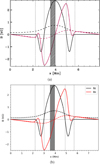 |
Fig. 1. Initial distribution of the magnetic field strength in the original (top) and our Bifrost (bottom) simulation. The magnetic field is shown at two horizontal cuts of the computational domain: at the base (z = 0 Mm, solid lines) and top (z = 1.26 Mm, dashed lines). The black and red lines indicate the vertical (Bz) and horizontal (Bx) magnetic field strengths, respectively. The vertical dotted lines indicate the three different segments of Bz where the flux is either positive (∼2 Mm wide) or negative (∼750 km wide). The shaded area indicates the location of the 400 km wide piston. This plot is for the strong field case. For the weak field, the field strengths are divided by 4 everywhere. |
Without the exact formula used for the initial Bz(z = 0), we approximated the initial Bz(z = 0) by sight and used a potential field extrapolation to construct the rest of the field.
In Figure 1b, we show our closest approximation to the original magnetic field configuration (Figure 1a). The only difference of note is that the Bifrost magnetic field strength decreases faster lower down in the atmosphere before flattening off higher up; whereas in the cited work, the decrease is more gradual with height. That means the magnetic field is slightly weaker in our Bifrost simulation than in the original OSC experiment. Consequently, any wave travelling with the Alfvén velocity vA will be moderately slower travelling upwards in the Bifrost simulation than in the original. Beyond this variation, the new magnetic field does not cause the waves to behave differently from the waves in the original experiment.
2.3. Boundary conditions
At the bottom boundary, the velocity was set to zero everywhere except for the 400 km wide area of the piston (x ∈ [3.55, 3.95] Mm, see the shaded area in Figure 1). The piston is a sinusoidal wave driver of the form
 (5)
(5)
where u* = uz for a radial driver and u* = ux for the transverse driver. The frequency was set to ω = 42.0 mHz, which is approximately ten times higher than both the acoustic cut-off frequency and the Brunt-Väisälä frequency (see Table 2). The amplitude, u0, was set to 400 m/s for the radial piston. In the original experiment, u0 = 400 m/s for the transverse piston as well. The authors noted, however, that the incoming waves get damped exponentially from 400 m/s to 125 m/s in the first 5–7 grid cells directly above the piston. Hence, the maximum Mach numbers are only a third of the expected 0.0047. This is purely a numerical artefact, which they compared to a ‘viscous boundary layer’ or a partially engaged ‘numerical clutch’ between the piston and magnetised plasma. In our Bifrost simulation, we experienced a similar damping of the waves, but not to the same extent. When driving transverse waves with an initial amplitude of 400 m/s, the waves were damped exponentially to around 250 m/s. As this is purely a numerical artefact, and not a physical phenomenon, we did not see any reason to try to recreate exactly the same effect. Instead, we reduced the initial amplitude of the transverse piston to u0 = 186 m/s so that the waves are damped to 125 m/s above the bottom 30 km. This means our simulation is comparable to the OSC simulation beyond this aspect.
Periodic boundary conditions were imposed on the horizontal boundaries. For the vertical boundaries, the original experiment imposed characteristic boundary conditions as described in Korevaar (1989). These were designed to allow waves into the computational grid at the lower boundary and to let acoustic waves through the upper boundary to minimise reflection (Rosenthal et al. 2002; Bogdan et al. 2003). In Bifrost, more general characteristic boundary conditions are implemented for the upper boundary and there is no characteristic boundary for the bottom. Instead of using Korevaar’s highly specialised boundary conditions, we used a perfectly reflecting upper boundary.
For the lower boundary, we applied slightly different boundary conditions for the radial and transverse pistons. For these simulations, we used a lower boundary, where waves going out of the box are allowed to do so while they are undergoing damping. For the transverse piston, the horizontal flows of the wave driver also create vertical flows at the piston boundaries. When applying the same boundaries as for the radial piston, the vertical flows at the piston edge reached amplitudes 1.5 times larger than the piston amplitude, which is not consistent with the results of the original work. Thus, we used the same reflecting boundaries on the lower boundary as for the upper when driving waves in the x-direction. This reduced the vertical flows at the piston boundaries to a fraction of the piston amplitude.
Due to our slightly simplified boundary conditions, we could see more of the waves being reflected at the upper and lower boundaries, compared to that seen in the original study. However, even with highly specialised boundary conditions, Bogdan et al. (2003) also experienced wave reflection. We found that the Bifrost wave behaviour after being reflected matched that of the original simulation, only with higher amplitudes. Therefore, we found that we could still use the Bogdan et al. (2003) analysis after the first wave has hit the upper boundary and this slight difference would not influence our results.
2.4. Wave mode identification scheme
As our simulation includes both a magnetic field and gravity, the fast and slow waves that become excited are magnetoacoustic gravity waves. In Table 3, we present the relevant characteristics of the fast and slow MAG waves for the high- and low-β plasmas for ease of reference.
Fast and slow magnetoacoustic gravity waves (modified version of Table 4 in Bogdan et al. 2003).
Bogdan et al. (2003) used u∥/c0 and u⊥/c0 to isolate the features for the fast and slow waves, where, u∥ and u⊥ are the velocity parallel and perpendicular to the magnetic field, respectively, and c0 = 8.49 km/s is the initial sound speed. These velocity components and the density perturbations Δρ/ρ0 = (ρ(x, z, t)−ρ(x, z, t = 0))/ρ(x, z, t = 0) are the three main values used for wave analysis in the original study.
The parallel and perpendicular velocity components isolate the longitudinal and transverse waves, respectively. To a large extent, this allows for the isolation of the fast and slow wave modes as they cross the magnetic canopy.
Both the original OSC and our experiments are done in 2D, which offers two big advantages for the wave analysis: (1) by definition, there is no Alfvén wave mode present, hence, we are only concerned with two wave modes; and (2) u∥ and u⊥ are well-defined. In 3D, these advantages, which make the Bogdan et al. (2003) analysis possible, are no longer true. Three wave modes will be present and only the parallel vector is well-defined. There is an uncountable number of possibilities for the two vectors perpendicular to the magnetic field, which are needed to form a basis for the vector space.
In Raboonik (2022), one possible method for identifying the fast, slow, and Alfvén wave modes in 3D is outlined. The wave mode identification variables are given by
 (6)
(6)
 (7)
(7)
 (8)
(8)
where e∥ = B/B is the unit vector parallel to the magnetic field. νA corresponds to the Alfvén wave mode. For a high-β plasma ν∥ and ν⊥ largely correspond to the fast and slow waves, respectively. For a low-β plasma this switches (like u∥/c0 and u⊥/c0 do in Bogdan et al. 2003). However, we note that these quantities do not correspond to the rigorous definition of each mode but are instead derived from known characteristics of the wave modes (compressibility and direction of propagation), again similar to how u∥/c0 and u⊥/c0 largely identify the direction of perturbation. They are meant as a tool for determining the type and location of waves.
We replicated the wave analysis in Bogdan et al. (2003) with both u∥/c0 and u⊥/c0 and with ν∥ and ν⊥. We used this comparison to investigate their usefulness and gain insight into what information they convey beyond the location of the possible wave modes. In this paper, we focus mainly on one of the simulations (the strong field and radial driving case). Before comparing the sets of components, we describe the differences from the original simulation caused by the simplified boundary conditions and slight differences in the magnetic field configuration. Then, we provide an in-depth analysis of what these components depict.
The WMIs are given in units of 1/time. To make an optimal comparison between the WMIs and the non-dimensional velocity components u∥/c0 and u⊥/c0, we kept the WMIs in the dimensionless form used by the numerical code. That is, we show ν* × [t] where [t] = 100 s. In the present work, to determine the physical units of ν*, we would simply multiply ν* with 1/[t] = 1/100 s. Furthermore, for the contour plots of ν*, we chose colour ranges that ignore extreme values at the piston boundary to best reveal the details of the WMIs.
3. Results: strong field and radial driving
The first case covered in Bogdan et al. (2003) uses a strong magnetic field (see Figure 1b) and a radial piston (starting with a compression into the domain). As in the approach in Bogdan et al. (2003), we focus much of our analysis on this case. There are two reasons for this. First, the strong field + radial driving case highlights the slight differences in our Bifrost simulation compared to the original OSC simulation (discussed in Section 2.1). We briefly point out these variations as well as discuss the findings of the original paper. Second, out of all the cases in Bogdan et al. (2003), this case best showcases the similarities between the velocity components u*/cS used by Bogdan et al. (2003) and our WMIs ν* components (where ∈(∥,⊥)). Along with these similarities, this case also highlights some interesting differences between the sets of components. These differences demonstrate that although the respective components are designed to isolate the same features, they are not identical and the information they convey must be interpreted differently.
We performed similar analyses on the other three cases in Bogdan et al. (2003). However, the objective of our study is to compare our wave mode identification scheme to that of the original study – and not to repeat the work of Bogdan et al. (2003). The results from our analysis of the other three cases only serve to underline the findings we present here in detail and it would quickly become repetitive. Therefore, we include a brief comparison analysis of the remaining three cases as an appendix.
3.1. Slow waves and the parallel components
In Figure 2, we show a comparison of u∥/c0 from the original paper (left) and from using the new Bifrost simulation (right), both at t = 58.5 seconds. The similarities between the trajectories of the magnetic field lines in the original and the new Bifrost simulation confirm that our estimate of the magnetic field (discussed in Section 2.2) is accurate. The white lines are iso-β lines with the thicker white lines indicating the β = 1 layer. In this instance (for the strong field configuration) the magnetic canopy is situated towards the sides of the grid. Here, we note that for the original simulation (left), the β = 100.00 line intersects the x = 0 Mm axis just below z = 0.4 Mm, while for the Bifrost simulation (right), this happens just above z = 0.4 Mm. It is a minor detail that does not affect the wave behaviour, but does inform us that the field in the original simulation is slightly stronger at this height than in the Bifrost simulation (as discussed in Section 2.2). Lastly, we note that the red vertical line at x = 3.81 Mm is the cut through which all the time-distance plots included in this paper have been taken, except Figure 8.
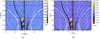 |
Fig. 2. Comparison of u∥/c0 from the original simulation (left) and the Bifrost simulation (right) of at t = 58.5 s. The colour range is the same for the two figures. The thin black lines indicate random magnetic field lines where the two thick black lines indicate the magnetic field lines attached to the edges of the piston. The thin white lines indicate iso-plasma β contours labelled by their respective values. The thick white lines indicate the layer where β = 1. The red lines are reference lines, at (horizontal) z = 499 km, z = 933 km and (vertical) x = 3.81 Mm. |
For the strong field configuration, the piston is situated in a low plasma-β atmosphere where the parallel components mainly isolate the longitudinal slow waves travelling along the magnetic field. At 58.5 seconds, the piston has just started its third period, and an object travelling vertically with the sound speed will have reached z = 498 km. Indeed, in both simulations, the leading wave has reached this point. These slow waves are always contained within the piston edge magnetic field line, so they never cross the magnetic canopy. However, the compressive part of the waves starts to overtake the rarefied part of the wave and, hence, the waves will steepen, forming shocks with time.
3.2. Comparison of u∥/c0 and ν∥
Having established that the difference between our Bifrost set-up and the original set-up of Bogdan et al. (2003) is mostly negligible, we now compare ν∥ (left) and u∥/c0 (right) at t = 58.5 s in Figure 3. Both use the same Bifrost data as in Figure 2b, but we have zoomed in on the wave and applied a more realistic aspect ratio. We note that u∥/c0 is identical to Figure 2b, but using a different colour scheme and range. In the middle panels, both components are overplotted by ν∥ = ±0.5 lines and in the bottom panels, both plots are overplotted by u∥/c0 = ±0.01 lines. These lines are drawn to frame the positive and negative sections of their respective values and ease comparisons between the two components.
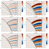 |
Fig. 3. ν∥ (left) and u∥/c0 (right) shown in the top panel for the strong field and radial driving case at t = 58.5 s. In the middle panel, both components are overplotted by black lines of ν∥ = ±0.5. In the bottom panel, both plots are overplotted by black lines of u∥/c0 = ±0.01. Red, black (non-contours) and white lines are as in Figure 2. Note: we have only kept the magnetic field lines anchored at the piston edges (black lines) and the β = 1 line for the two bottom plots for simplicity. We also note that the colour range is different for the two variables. |
Unsurprisingly, both components indicate that the leading wave has reached a height of z = 0.498 Mm. However, while u∥/c0 (right) is characterised by positive and negative bands of similar vertical extension (from the sinusoidal wave driver), ν∥ (left) shows a vertical narrowing of the negative bands and broadening of the positive bands with altitude. This reflects the steepening of the waves with height as the compressive part of the wave overtakes the rarefied part.
In the middle row of Figure 3, lines of ν∥ = ±0.5 frame the positive and negative bands of ν∥ (middle left). We see that the sections where positive and negative lines border each other, namely, where ν∥ changes sign, quite accurately trace the peaks of u∥/c0 in the middle right panel.
Intuitively, this makes sense as ν∥ = ∇ ⋅ (u∥e∥) is based on derivatives, and one of the most fundamental properties of derivatives is that they are zero where a curve reaches a maximum or minimum. Using the same basic knowledge about derivatives, it should come as no surprise that when we study lines of u∥/c0 = ±0.01 on top of the ν∥ contour (bottom left), we see that where u∥/c0 changes sign is also where ν∥ achieves its largest magnitudes of each wave segment. Again, this intuitively makes sense as the gradient of the sinusoidal wave driver is largest where the sine function is equal to zero. This correspondence between u∥/c0 changing signs and ν∥ peaking is not a universal result, but a nice coincidence that makes our analysis more intuitive.
From our analysis of all four cases, it is evident that where ν* changes signs indicates a wave peak. In most cases, considering the positive direction of the grid and knowledge about the magnetic field let us deduce if a wave peak is a maximum or minimum.
In Figure 3, where positive and negative bands of ν∥ neighbour each other vertically, we can see a simple example of this. Here, both the magnetic field and the positive z-direction are directed upwards. Just above the piston, we see a positive band of ν∥ with a negative band just above it. This indicates an increase and then decrease of the velocity, namely, a positive peak. This is reflected in u∥/c0 (right). We can follow this pattern upwards with the other positive and negative bands. If the magnetic field had been pointing downwards, this would instead have been a minimum.
3.3. Fast MAG waves and crossing the β = 1 line
The radial piston also excites low-β MAG fast waves, although much weaker than the slow waves. In a low-β plasma, the fast waves travel with a velocity close to the Alfvén speed ( ) and they are not constrained to the magnetic field. Hence, contrary to the slow MAG waves, the fast waves will eventually encounter the magnetic canopy. To isolate the fast wave, we use the perpendicular components ν⊥ and u⊥/c0.
In Figure 4 we compare ν⊥ (left) and u⊥/c0 (right) at t = 29.9 s. On top of both contours, lines of ν⊥ = ±0.01 are drawn to indicate the main non-zero sections of ν⊥. In both contours, we see the characteristic horseshoe shape as in the original paper. We see in the leading wave how ν⊥ indicates a peak down the right ‘leg’ of the arch-like wave. Both components indicate three sections of the wave, namely: two maxima and one minimum in the middle. The arch-like shape of the fast waves is due to the strong magnetic field strength in the centre of the domain, which weakens towards the edges. Over time, the centre of the fast wave is accelerated through the top of the grid. The decreasing magnetic field strength away from the midpoint leaves the ‘legs’ of the arch-like fast waves to drift horizontally towards the magnetic canopy. This is shown in Figure 5, which displays the perpendicular components at t = 58.5 s (same time as Figures 2 and 3). In Figure 5, we note that ν⊥ ≈ 0 in the upper centre of the grid (along x = 3.81 Mm for z > 0.7 Mm). To the left of this band, ν⊥ is positive, and to the right, ν⊥ is negative. Hence, this indicates a broad, positive wave peak, which is confirmed by u⊥/c0.
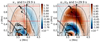 |
Fig. 4. Comparison of ν⊥ (left) and u⊥/c0 (right) for the strong field and radial driving case after t = 29.9 seconds. Black lines of ν⊥ = ±0.01 are overplotted on both graphs. The red, white, and black (non-contour) lines are the same as in Figure 2. |
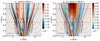 |
Fig. 5. Comparison of ν⊥ (left) and u⊥/c0 (right) for strong field and radial driving after t = 58.5 seconds. Black lines of u⊥/c0 = ±0.001 are overplotted on both graphs. |
As time progresses, the horizontally moving low-β fast waves will cross the magnetic canopy. In Figure 6, we show ν⊥ zoomed in on the lower left corner of the grid at t = 100.1 s. This is after a full period of the incoming wave has been transmitted across the canopy. On top of ν⊥, lines of u⊥/c0 = ±0.001 are plotted to indicate the main non-zero segments u⊥/c0. The ‘legs’ of the fast waves are almost parallel to the magnetic canopy as it approaches from the low-β plasma. Across the whole magnetic canopy, the low-β fast wave is transmitted into a high-β fast wave. The perpendicular WMI in Figure 6 captures these high-β fast waves only in the upper section of the plot (for z > 0.4 Mm) as in this region the wave vector and the magnetic field are almost perpendicular. Below z = 0.4 Mm, the magnetic field is almost aligned with ∇β and, hence, the fast wave shows up in the parallel WMI (not shown here). In this region, the perpendicular component shows wave trains of transmitted high-β, transversal slow waves. Since slow waves are guided along the magnetic field, the low-β fast waves are only converted to transmitted high-β slow waves where the magnetic field is aligned with ∇β.
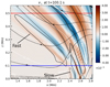 |
Fig. 6. Zoomed in cut of ν⊥ for the strong field and radial driving case after t = 101.1 seconds. Black lines of u⊥/c0 = ±0.001 are overplotted to indicate the location of positive and negative areas of u⊥/c0 (same format as bottom left panel in Figure 3). Red, black (non-contour) and white lines are as in Figure 2. The blue horizontal line indicates the line through which we take the time-distance plot in Figure 8. |
Hence, the sections between z = 0.1 and 0.4 Mm are the only sections where slow waves are transmitted into the high-β plasma. Overplotted on ν⊥, we show contours of the corresponding u⊥/c0 = ±0.001, which indicate the main negative and positive segments of u⊥/c0. We see that where ν⊥ changes sign largely falls within the centre of these u⊥/c0 segments, where u⊥/c0 reaches a maximum or minimum.
3.4. Time-distance plots
In Figure 7, we show time-distance plots of ν∥ (top) and ν⊥ (bottom) along x = 3.81 Mm (the red vertical line in, for example, Figure 2). The solid black line indicates the location of an object travelling from the bottom boundary with the constant initial sound speed (c0 = 8.49 km/s). For example, from Figure 2, we can see that the cut through which we take the time-distance plot is almost aligned with the magnetic field and the slow MAG waves should follow this trajectory closely. The curved black line (from the origin) indicates the trajectory of an object travelling vertically with the Alfvén velocity. The dashed black lines are placed to indicate the trajectory of a downwardly propagating wave travelling with the sound speed. The leftmost is placed at the location where the fast MAG waves reach z = 1.2 Mm and the rightmost where the slow MAG wave does the same.
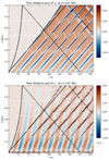 |
Fig. 7. Time-distance plots of ν∥ (top) and ν⊥ (bottom) along x = 3.81 Mm. The red and white lines are as in Figure 2. From the origin, a straight diagonal line represents the trajectory of an object travelling with the initial sound speed c0 = 8.49 km/s and a curved black line indicates the position of an object travelling vertically with the Alfvén velocity. The dashed and dash-dotted lines indicate the trajectory of an object travelling with the negative initial sound speed. |
In the parallel WMI (top), we see the steepening of the waves with time. This steepening creates such large values that they are also visible in the perpendicular WMI (bottom). Looking beyond these sharp lines in ν⊥, we can clearly make out the positive and negative bands of the fast MAG waves travelling upwards with the Alfvén velocity. These bands remain much more constant in width, indicating very little steepening of fast MAG waves with height.
In Figure 8, we show another time-distance plot, this time at z = 0.1 Mm in the x-range of x ∈ [0.1, 2.84] Mm (this line is indicated in blue in Figures 4 and 5). This is mainly the high-β plasma on the left of the piston. This time-distance plot shows the two wave modes being transmitted from the low-β fast wave. Unlike the previous plot, this time-distance plot is not aligned with the magnetic field. Between approximately x = 2.35 Mm and x = 3.75 Mm, where slow waves are being transmitted, we see the waves decelerate due to the diminishing magnetic field strength (and hence the decreasing Alfvén velocity). For x < 2.35 Mm, we see the transmitted fast waves travelling with the sound speed.
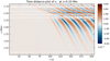 |
Fig. 8. Time-distance plot of ν⊥ along z = 0.1 Mm for 1.0 ≤ x ≤ 2.84] Mm. White lines are iso-beta lines, with the thick one being β = 1. |
4. Discussion and conclusion
As the interest for reliable MHD wave mode identification schemes is growing, careful and detailed analyses of such schemes are needed to establish what the scheme conveys, as well as to test its robustness, scope, and potential pitfalls. In this paper, we present an in-depth analysis of an MHD wave mode identification scheme. We have shown that for fast and slow MAG waves, the WMIs isolate the expected features in both high- and low-β plasmas. We did this by recreating the piston experiment of Bogdan et al. (2003), using the numerical simulation code Bifrost. In this 2D experiment, fast and slow waves are driven into a realistic stratified atmosphere through a piston imposed at the lower boundary. We have shown that for fast and slow MAG waves, the WMIs isolate the expected features in both high- and low-β plasmas. We used the Bogdan et al. (2003) analysis of fast and slow waves to verify our scheme. We also found that, apart from the locations of the two wave modes, the WMIs can also provide valuable information about the wave peaks and steepening.
Using the velocity components that are parallel and perpendicular to the magnetic field makes sense in a 2D domain. In 3D, however, it is not a valid scheme for similar wave analyses, as the perpendicular direction u⊥ is not well defined; additionally, in 3D we also get Alfvénic wave modes. This is not to say there are no methods available for a 3D decomposition of the velocity field. For clearly defined geometries such as a cylinder or torus (often used for CMEs), it is possible to define a coordinate system along the magnetic field (e∥), normal to the surface (eS) and the cross product (e∥ × eS) of these (see e.g. Chapter 17 in Goedbloed et al. 2019). Toroidal coordinates are often used when modelling CMEs, but they are not suited for our case, where we do not have a clear geometry such as a flux tube to guide the waves. It would also be hard to generalise this for a realistic simulation of the solar atmosphere. A frequently used scheme in wave research is the Frenet-Serret frame-of-reference (Frenet 1852; Serret 1851), where the basis (T, N, P) is defined by the unit vector tangent to the magnetic field, T = e∥, N points in the direction of the curve, and P = T × N. However, a common issue with these examples is that it is not clear how each of these basis vectors relates back to one-wave mode. In particlar, the compressive magnetic MAG mode and the Alfvén mode are difficult to distinguish between with a vector scheme (e.g. Carlsson & Bogdan 2006)
In this work, we tested a set of three wave-mode identification components: ν∥ = ∇ ⋅ (u∥e∥), ν⊥ = ∇ ⋅ u − ν∥, and νA = ∇ × u ⋅ e∥. These (or other, very similar) components have already been applied in some previous studies (e.g. Leenaarts & Carlsson 2015; Cally 2017; Khomenko et al. 2018) as a potential indicator of MHD waves. However, little research has been conducted looking at what exactly can be deduced from this scheme. The WMIs are mathematically designed to draw out features of the fast, slow, and Alfvén MHD modes. Similarly to u∥ and u⊥, these WMI components isolate the direction of perturbation. In addition, they also consider the compressibility of the waves. This addition allows for the detection of incompressible Alfvén waves in 3D. However, since our simulation is strictly 2D, the Alfvén component, νA, is zero throughout. Furthermore, the WMI components never follow a perpendicular direction and only consider parallel and non-parallel motions. This makes them well-suited for isolating wave modes in 3D. Still, it is unclear what physical properties we can deduce from them, if any. By using the Bogdan et al. (2003) experiment as a base case, we have shown that we can, in fact, learn more than previously thought from this scheme.
The main difference between (u∥, u⊥) and (ν∥, ν⊥) is that the WMIs are based on derivatives. Since ν∥ = ∇ ⋅ (u∥e∥) depends on u∥, they will largely pick up the same features. Here, ν⊥ captures all the compressive parts of u that are not perturbing parallel to the magnetic field. In 2D, this is reduced to ν⊥ = ∇ ⋅ (u⊥e⊥). The 2D study has made it possible to meticulously analyse how we can relate features of the WMI data back to MAG wave modes. The use of scalars, rather than a vector field, means we lose the possibility to deduce certain physical properties of the wave, such as the perturbation direction. However, by comparing the WMI to the thorough wave analysis by Bogdan et al. (2003), we have shown that we are often able to deduce more information about the wave than just their potential presence.
We can use basic knowledge about derivatives to deduce wave features from the WMIs, in particular, the location of peaks (where ν*-pagination
changes sign) and of steepening (narrow bands of strong magnitude), as seen in Figure 3. In many cases, we can also determine whether this is a maximum or minimum by considering the direction of the local magnetic field. These are guidelines, not rules, as there are exceptions. Yet, if we were to strictly follow these guidelines when interpreting ν∥ and ν⊥ in this study, we would gain an accurate overview of the fast and slow wave modes, comparable to the velocity components used in Bogdan et al. (2003).
This WMI scheme mostly applies to simulations, and its usage in observations is not yet clear. Enerhaug et al. (2024) provides a proof-of-concept for how the Alfvén component can be applied to observations (in the corona) but states that a similar method would be difficult for ν⊥ and ν∥. However, a wave mode identification scheme for simulations is highly desirable. A substantial part of MHD wave research is simulation-based (e.g. Goossens et al. 2009; Pascoe et al. 2010; De Moortel & Howson 2022; Callingham et al. 2024; Soler & Hillier 2025; Kohutova & Popovas 2021, to name a few). These studies often aim to study the energy transport of the waves. As each wave mode is associated with a different energy budget and dissipation process, having a reliable WMI scheme would be a very valuable tool in this research. Furthermore, simulations are frequently used to study observations using forward modelling. By producing simulations for which the synthetic observables match observations, we can analyse the simulation in detail to gain a deeper understanding of the observed phenomena. Forward modelling has been used for studying wave modes in the sun (e.g. Antolin & Van Doorsselaere 2013; Yuan & Van Doorsselaere 2016; Yuan et al. 2015; Fyfe et al. 2020) and in the related research area of coronal seismology (e.g. Uchida 1970; Roberts et al. 1984; Taroyan & Erdélyi 2009; Chen & Peter 2015; Pascoe et al. 2018; Karamimehr et al. 2019). Therefore, even though the WMIs we describe here are used only in simulations, they can also be (indirectly) useful for observational studies.
Following this work, several questions for a 3D study have emerged. On an analytical level, we must consider whether we can still deduce the maximum, minimum, and steepening of the wave from the WMIs when adding a third dimension? Additionally, since the WMIs are based on derivatives, they are much more sensitive to fluctuations and small changes in the simulation compared to u∥ and u⊥. In our simulation, a consequence of this sensitivity was some very large values around the piston edges. To draw out the interesting details of the WMIs, we adjusted our colour range to ignore these large values. The real solar atmosphere is subject to a multitude of parallel processes, creating both small and large-scale changes in the plasma. Therefore, interpreting the WMIs could require greater care in more realistic, full 3D simulations of the solar atmosphere. Lastly, as the WMIs are made to isolate features of the wave modes, not the wave modes themselves (likewise to the case of u∥ and u⊥ in Bogdan et al. 2003), it will be important to examine the WMIs in relation to each other over time. This will be addressed in the second paper in this series.
Acknowledgments
This research has been supported by the Research Council of Norway through its Centres of Excellence scheme, project number 262622. E.E. received funding from the University of St Andrews Global Fellowship Scheme.
References
- Anfinogentov, S. A., & Nakariakov, V. M. 2019, ApJ, 884, L40 [CrossRef] [Google Scholar]
- Anfinogentov, S. A., Antolin, P., Inglis, A. R., et al. 2022, Space Sci. Rev., 218, 9 [NASA ADS] [CrossRef] [Google Scholar]
- Antolin, P., & Van Doorsselaere, T. 2013, A&A, 555, A74 [NASA ADS] [CrossRef] [EDP Sciences] [Google Scholar]
- Arregui, I. 2015, Philos. Trans. R. Soc. Lond. Ser. A, 373, 20140261 [Google Scholar]
- Bogdan, T. J., Carlsson, M., Hansteen, V. H., et al. 2003, ApJ, 599, 626 [Google Scholar]
- Callingham, H., De Moortel, I., & Pagano, P. 2024, MNRAS, 535, 1640 [Google Scholar]
- Cally, P. S. 2017, MNRAS, 466, 413 [NASA ADS] [CrossRef] [Google Scholar]
- Carlsson, M., & Bogdan, T. J. 2006, Philos. Trans. R. Soc. Lond. Ser. A, 364, 395 [Google Scholar]
- Chen, F., & Peter, H. 2015, A&A, 581, A137 [NASA ADS] [CrossRef] [EDP Sciences] [Google Scholar]
- De Moortel, I. 2005, Philos. Trans. R. Soc. Lond. Ser. A, 363, 2743 [Google Scholar]
- De Moortel, I., & Howson, T. A. 2022, ApJ, 941, 85 [NASA ADS] [CrossRef] [Google Scholar]
- De Pontieu, B., Carlsson, M., Rouppe van der Voort, L. H. M., et al. 2012, ApJ, 752, L12 [Google Scholar]
- Duckenfield, T. J., Goddard, C. R., Pascoe, D. J., & Nakariakov, V. M. 2019, A&A, 632, A64 [NASA ADS] [CrossRef] [EDP Sciences] [Google Scholar]
- Enerhaug, E., Howson, T. A., & De Moortel, I. 2024, A&A, 681, L11 [NASA ADS] [CrossRef] [EDP Sciences] [Google Scholar]
- Frenet, F. 1852, J. Math. Pures Appl., 17, 437 [Google Scholar]
- Fyfe, L. E., Howson, T. A., & De Moortel, I. 2020, A&A, 643, A86 [NASA ADS] [CrossRef] [EDP Sciences] [Google Scholar]
- Goedbloed, J. P., Goedbloed, H., Keppens, R., & Poedts, S. 2019, Magnetohydrodynamics: of laboratory and astrophysical plasmas (Cambridge University Press) [Google Scholar]
- Goossens, M., Terradas, J., Andries, J., Arregui, I., & Ballester, J. L. 2009, A&A, 503, 213 [NASA ADS] [CrossRef] [EDP Sciences] [Google Scholar]
- Goossens, M., Van Doorsselaere, T., Soler, R., & Verth, G. 2013, ApJ, 768, 191 [NASA ADS] [CrossRef] [Google Scholar]
- Gudiksen, B. V., Carlsson, M., Hansteen, V. H., et al. 2011, A&A, 531, A154 [NASA ADS] [CrossRef] [EDP Sciences] [Google Scholar]
- Hansteen, V. H. 2004, in Multi-Wavelength Investigations of Solar Activity, eds. A. V. Stepanov, E. E. Benevolenskaya, & A. G. Kosovichev, IAU Symposium, 223, 385 [Google Scholar]
- Jess, D. B., Jafarzadeh, S., Keys, P. H., et al. 2023, Liv. Rev. Sol. Phys., 20, 1 [NASA ADS] [CrossRef] [Google Scholar]
- Karamimehr, M. R., Vasheghani Farahani, S., & Ebadi, H. 2019, ApJ, 886, 112 [Google Scholar]
- Khan, J. I., & Aurass, H. 2002, A&A, 383, 1018 [NASA ADS] [CrossRef] [EDP Sciences] [Google Scholar]
- Khomenko, E., & Cally, P. S. 2011, Journal of Physics Conference Series, 271, 012042 [Google Scholar]
- Khomenko, E., & Cally, P. S. 2012, ApJ, 746, 68 [Google Scholar]
- Khomenko, E., Vitas, N., Collados, M., & de Vicente, A. 2018, A&A, 618, A87 [NASA ADS] [CrossRef] [EDP Sciences] [Google Scholar]
- Kohutova, P., & Popovas, A. 2021, A&A, 647, A81 [NASA ADS] [CrossRef] [EDP Sciences] [Google Scholar]
- Korevaar, P. 1989, A&A, 226, 209 [Google Scholar]
- Leenaarts, J., & Carlsson, M. 2015, & Rouppe van der Voort. L., ApJ, 802, 136 [Google Scholar]
- Morton, R. J., Tiwari, A. K., Van Doorsselaere, T., & McLaughlin, J. A. 2021, ApJ, 923, 225 [NASA ADS] [CrossRef] [Google Scholar]
- Pascoe, D. J., Wright, A. N., & De Moortel, I. 2010, ApJ, 711, 990 [Google Scholar]
- Pascoe, D. J., Anfinogentov, S. A., Goddard, C. R., & Nakariakov, V. M. 2018, ApJ, 860, 31 [Google Scholar]
- Pascoe, D. J., Van Doorsselaere, T., & De Moortel, I. 2022, ApJ, 929, 101 [NASA ADS] [CrossRef] [Google Scholar]
- Raboonik, A. 2022, Ph.D. Thesis, Monash University, Australia [Google Scholar]
- Roberts, B., Edwin, P. M., & Benz, A. O. 1984, ApJ, 279, 857 [CrossRef] [Google Scholar]
- Rosenthal, C., Bogdan, T., Carlsson, M., et al. 2002, ApJ, 564, 508 [Google Scholar]
- Serret, J.-A. 1851, J. Math. Pures Appl., 16, 499 [Google Scholar]
- Shelyag, S., Khomenko, E., de Vicente, A., & Przybylski, D. 2016, ApJ, 819, L11 [Google Scholar]
- Soler, R., & Hillier, A. 2025, A&A, 693, A201 [NASA ADS] [CrossRef] [EDP Sciences] [Google Scholar]
- Stein, R. F., Nordlund, Å., Collet, R., & Trampedach, R. 2024, ApJ, 970, 24 [NASA ADS] [CrossRef] [Google Scholar]
- Taroyan, Y., & Erdélyi, R. 2009, Space Sci. Rev., 149, 229 [Google Scholar]
- Uchida, Y. 1970, PASJ, 22, 341 [NASA ADS] [Google Scholar]
- Van Doorsselaere, T., Srivastava, A. K., Antolin, P., et al. 2020, Space Sci. Rev., 216, 140 [Google Scholar]
- Yadav, N., Keppens, R., & Popescu Braileanu, B. 2022, in 44th COSPAR Scientific Assembly. Held 16-24 July, 44, 2546 [Google Scholar]
- Yuan, D., & Van Doorsselaere, T. 2016, ApJS, 223, 24 [NASA ADS] [CrossRef] [Google Scholar]
- Yuan, D., Van Doorsselaere, T., Banerjee, D., & Antolin, P. 2015, ApJ, 807, 98 [NASA ADS] [CrossRef] [Google Scholar]
Appendix A: Findings from the other cases
A.1. Weak field and radial driving
For the weak field, the simulation was set up identically to the simulation analysed in Section 3, except that the initial magnetic field is reduced by a factor of 4 everywhere. As we see in Figure A.1, in such a configuration, the piston is located in a high-β plasma. The upward propagating waves cross into a low-β plasma across a roughly semi-horizontal magnetic canopy located around z = 0.6 Mm. Below the magnetic canopy, in the high-β plasma, the longitudinal waves are now mainly fast, and the transverse waves mainly slow. The parallel components ν∥ (left) and u∥/c0 (right) at t = 58.5 s are shown in the top panels of Figure A.1, illustrating the fast wave just as it is about to cross the magnetic canopy.
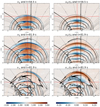 |
Fig. A.1. Comparison of the WMI (left) and velocity (right) components at two different times for the weak field with radial driving simulation. The top panels show the parallel components ν∥ (top left) and u∥/c0 (top right) at t = 58.5 s. The middle panels show the parallel components ν∥ (middle left) and u∥/c0 (middle right) at t = 81.9 s. The bottom panels show the perpendicular components ν⊥ (bottom left) and u⊥/c0 (bottom right) also at t = 81/.9 s. For each row, lines of the respective ν* = ±0.05 are overplotted to make comparison between the figures easier. Red, black (non-contour) and white lines are as in Figure 2. |
In the middle and bottom panels of Figure A.1, we show the parallel and perpendicular components, respectively, at t = 81.9 s. They depict how the high-β fast waves are being transmitted into both low-β slow waves (parallel components, middle panel) and low-β fast waves (perpendicular components, bottom panel). At 81.9 s, the outline of the leading fast wave, above the leading slow wave, is captured by both the parallel and perpendicular components (middle and bottom panels). Note also that the perpendicular components capture the slightly off-centre wavefront apex of the low-β fast waves, a phenomenon caused by the interference of the imposed radial piston and the two artificial, out-of-phase transverse pistons at the piston boundary. These artificial transverse pistons are also the reason for the slightly complex interference pattern we see from below the magnetic canopy in both the parallel and perpendicular components.
For each row of panels in Figure A.1, we have overplotted lines of the relevant WMI ν* = ±0.05 to frame the main positive and negative segments of the WMI. In the parallel components (top and middle panels), we clearly see how the lines where ν∥ changes sign neatly trace the peaks of the waves in u∥/c0 (top and middle right). Furthermore, we note how ν∥, in the same way as u∥/c0, captures the arch-like shape of the fast wave, which is not contained within the magnetic field lines rooted in the piston boundary (thick black lines). In the perpendicular components (bottom panels), the lines of ν⊥ = ±0.05 can appear chaotic, but as u⊥/c0 (bottom right) confirms, the perpendicular components capture the complex interference pattern described above. Additionally, we note that the change of sign in ν⊥ largely corresponds to the peaks in u⊥/c0 and that both perpendicular components capture the emerging low-β fast wave above the magnetic canopy.
In Figure A.2, we show the time-distance plots of the parallel component ν∥ (top) and the perpendicular component ν⊥ (bottom) along x = 3.81 Mmn (red vertical line in Figure A.1). In the small region 0 < z < 0.1 Mm, the perpendicular component captures the high-β slow MAG wave, travelling with the Alfvén velocity. However, the wave receives a slight ’boost in the area between z = 0.1 Mm and 0.2 Mm. This ’boost’ in the perpendicular component is actually an earlier wave from the artificial, transverse piston edge at x = 3.55 Mm, which has drifted horizontally in the positive x-direction and reached x = 3.81 Mm at around z = 0.1 Mm.
For the parallel component (top), below the magnetic canopy, the high-β fast MAG wave mode is acoustic in nature. As the high-β fast wave crosses the magnetic canopy, we see both low-β fast (perpendicular component) and slow (parallel component) waves being transmitted. In the parallel component, the slow waves continue with the sound speed and steepen with height, similar to for the strong field case (see Section 3). In the perpendicular component, we see low-β fast waves transmitted, which accelerate with the Alfvén velocity (curved black line from the origin). In the same plot, we also see the reflected fast waves travel back down in the atmosphere.
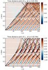 |
Fig. A.2. Comparison of the time-distance plot of ν∥ (top) and ν⊥ (bottom) along x = 3.81 Mm for a weak field with radial driving. From the origin, the black, diagonal, straight line indicates the trajectory of an object travelling vertically with the initial sound speed c0 = 8.49 km/s, and the black, curved line indicates the position of an object travelling with the Alfvén velocity. The diagonal dashed and dash-dotted lines indicate the trajectory of an object travelling with the negative initial sound speed. |
A.2. Weak field and transverse driving
We turn our attention to a transverse piston, first in the weak field case. Figure A.3, follows the format of Figure A.1, only at different times. The top panels of Figure A.3 show the parallel components ν∥ (left) and u∥/c0 (right) at t = 58.5 s. We see that the parallel components capture the high-β fast wave train travelling upwards. Overplotted on both panels are lines of ν∥ = ±0.005. As observed previously, the lines where ν∥ changes sign correspond to the peaks of u∥/c0 (top right). We also see this in the middle panel, where the parallel components are displayed at t = 123.5 s. In the bottom panel, we show the perpendicular components at t = 123.5 s. At t = 123.5 s, multiple wave periods have been transmitted across the magnetic canopy, and we see how ν∥ (middle left) captures the low-β slow wave and ν⊥ (bottom left) the fast wave, similar to their velocity counterparts.
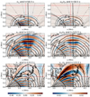 |
Fig. A.3. Comparison of the WMI (left) and velocity (right) components at two different times for the weak field with transverse driving simulation. The top panels show the parallel components ν∥ (top left) and u∥/c0 (top right) at t = 58.5 s. The middle panels show the parallel components ν∥ (middle left) and u∥/c0 (middle right) at t = 123.5 s. The bottom panels show the perpendicular components ν⊥ (bottom left) and u⊥/c0 (bottom right), also at t = 123.5 s. For each row, lines of the respective ν* = ±0.005 are overplotted. Red, black (non-contour) and white lines are as in Figure 2. |
In Figure A.4, we show the time-distance plots of the parallel (top) and perpendicular (bottom) WMI components along x = 3.81 Mm.
For β < 1, both components largely follow the Alfvén trajectory (curved black line from the origin). This is due to the low excitation of longitudinal waves by the transverse piston, which means the acoustic waves are very weak just above the piston. However, slightly higher, at z ≈ 0.2 Mm, we see a fast wave emerge in ν∥. At this height, the radial flows from the artificial piston at the piston edges have drifted across to x = 3.81 Mm and continue upwards. This effect is also the reason for the little ’boost,’ which we see in ν⊥ along z = 0.2 Mm. Hence, the waves we see in ν∥ (top) following the trajectory of the sound speed (black, diagonal line from the origin) are the high-β fast waves, which are being transmitted as low-β slow waves (or in other words, propagate as acoustic waves throughout). The waves we also see accelerate away in ν⊥ (bottom) are the high-β slow waves, which are transmitted across the magnetic canopy layer, into both low-β fast and slow waves. We also see that the negative bands in ν∥ are narrowing with height, indicating steepening with altitude.
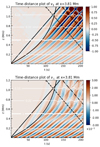 |
Fig. A.4. Comparison of the time-distance plot of ν∥ (top) and ν⊥ (bottom) along x = 3.81 Mm for a weak field with transverse driving. From the origin, the black, diagonal, straight line indicates the trajectory of an object travelling vertically with the initial sound speed c0 = 8.49 km/s, and the black, curved line indicates the position of an object travelling with the Alfvén velocity. The diagonal dashed and dash-dotted lines indicate the trajectory of an object travelling with the negative initial sound speed. |
A.3. Strong field and transverse driving
The strong field with transverse driving is the last of the experiments in Bogdan et al. (2003). Following their example, we keep this section brief, as there is little to comment on about the wave behaviour and the comparison to the WMIs confirms the findings we have discussed thus far. In Figure A.5, we plot the low-β fast wave at t = 27.3 s using the perpendicular components (top) and the low-β slow waves at t = 58.5 s using the parallel components (bottom). The bands framing the positive and negative sections of the WMI values confirm what we have seen so far:
-
where the WMI changes sign indicates a wave peak;
-
we can deduce whether this wave peak is a maximum or minimum by considering the positive directions of our grid;
-
we can deduce the steepening of the wave by the narrowing and broadening of the positive and negative bands.
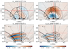 |
Fig. A.5. Comparison of the WMI (left) and velocity (right) components at two different times for the strong field with transverse driving simulation. The top panels show the perpendicular components ν⊥ (top left) and u⊥/c0 (top right) at t = 27.3 s. The bottom panels show the parallel components ν∥ (bottom left) and u∥/c0 (bottom right) at t = 58.5 s. For each row, lines of the respective ν* = ±0.02 are overplotted. Red, black (non-contour) and white lines are as in Figure 2. |
All Tables
Fast and slow magnetoacoustic gravity waves (modified version of Table 4 in Bogdan et al. 2003).
All Figures
|
Fig. 1. Initial distribution of the magnetic field strength in the original (top) and our Bifrost (bottom) simulation. The magnetic field is shown at two horizontal cuts of the computational domain: at the base (z = 0 Mm, solid lines) and top (z = 1.26 Mm, dashed lines). The black and red lines indicate the vertical (Bz) and horizontal (Bx) magnetic field strengths, respectively. The vertical dotted lines indicate the three different segments of Bz where the flux is either positive (∼2 Mm wide) or negative (∼750 km wide). The shaded area indicates the location of the 400 km wide piston. This plot is for the strong field case. For the weak field, the field strengths are divided by 4 everywhere. |
| In the text | |
|
Fig. 2. Comparison of u∥/c0 from the original simulation (left) and the Bifrost simulation (right) of at t = 58.5 s. The colour range is the same for the two figures. The thin black lines indicate random magnetic field lines where the two thick black lines indicate the magnetic field lines attached to the edges of the piston. The thin white lines indicate iso-plasma β contours labelled by their respective values. The thick white lines indicate the layer where β = 1. The red lines are reference lines, at (horizontal) z = 499 km, z = 933 km and (vertical) x = 3.81 Mm. |
| In the text | |
|
Fig. 3. ν∥ (left) and u∥/c0 (right) shown in the top panel for the strong field and radial driving case at t = 58.5 s. In the middle panel, both components are overplotted by black lines of ν∥ = ±0.5. In the bottom panel, both plots are overplotted by black lines of u∥/c0 = ±0.01. Red, black (non-contours) and white lines are as in Figure 2. Note: we have only kept the magnetic field lines anchored at the piston edges (black lines) and the β = 1 line for the two bottom plots for simplicity. We also note that the colour range is different for the two variables. |
| In the text | |
|
Fig. 4. Comparison of ν⊥ (left) and u⊥/c0 (right) for the strong field and radial driving case after t = 29.9 seconds. Black lines of ν⊥ = ±0.01 are overplotted on both graphs. The red, white, and black (non-contour) lines are the same as in Figure 2. |
| In the text | |
|
Fig. 5. Comparison of ν⊥ (left) and u⊥/c0 (right) for strong field and radial driving after t = 58.5 seconds. Black lines of u⊥/c0 = ±0.001 are overplotted on both graphs. |
| In the text | |
|
Fig. 6. Zoomed in cut of ν⊥ for the strong field and radial driving case after t = 101.1 seconds. Black lines of u⊥/c0 = ±0.001 are overplotted to indicate the location of positive and negative areas of u⊥/c0 (same format as bottom left panel in Figure 3). Red, black (non-contour) and white lines are as in Figure 2. The blue horizontal line indicates the line through which we take the time-distance plot in Figure 8. |
| In the text | |
|
Fig. 7. Time-distance plots of ν∥ (top) and ν⊥ (bottom) along x = 3.81 Mm. The red and white lines are as in Figure 2. From the origin, a straight diagonal line represents the trajectory of an object travelling with the initial sound speed c0 = 8.49 km/s and a curved black line indicates the position of an object travelling vertically with the Alfvén velocity. The dashed and dash-dotted lines indicate the trajectory of an object travelling with the negative initial sound speed. |
| In the text | |
|
Fig. 8. Time-distance plot of ν⊥ along z = 0.1 Mm for 1.0 ≤ x ≤ 2.84] Mm. White lines are iso-beta lines, with the thick one being β = 1. |
| In the text | |
|
Fig. A.1. Comparison of the WMI (left) and velocity (right) components at two different times for the weak field with radial driving simulation. The top panels show the parallel components ν∥ (top left) and u∥/c0 (top right) at t = 58.5 s. The middle panels show the parallel components ν∥ (middle left) and u∥/c0 (middle right) at t = 81.9 s. The bottom panels show the perpendicular components ν⊥ (bottom left) and u⊥/c0 (bottom right) also at t = 81/.9 s. For each row, lines of the respective ν* = ±0.05 are overplotted to make comparison between the figures easier. Red, black (non-contour) and white lines are as in Figure 2. |
| In the text | |
|
Fig. A.2. Comparison of the time-distance plot of ν∥ (top) and ν⊥ (bottom) along x = 3.81 Mm for a weak field with radial driving. From the origin, the black, diagonal, straight line indicates the trajectory of an object travelling vertically with the initial sound speed c0 = 8.49 km/s, and the black, curved line indicates the position of an object travelling with the Alfvén velocity. The diagonal dashed and dash-dotted lines indicate the trajectory of an object travelling with the negative initial sound speed. |
| In the text | |
|
Fig. A.3. Comparison of the WMI (left) and velocity (right) components at two different times for the weak field with transverse driving simulation. The top panels show the parallel components ν∥ (top left) and u∥/c0 (top right) at t = 58.5 s. The middle panels show the parallel components ν∥ (middle left) and u∥/c0 (middle right) at t = 123.5 s. The bottom panels show the perpendicular components ν⊥ (bottom left) and u⊥/c0 (bottom right), also at t = 123.5 s. For each row, lines of the respective ν* = ±0.005 are overplotted. Red, black (non-contour) and white lines are as in Figure 2. |
| In the text | |
|
Fig. A.4. Comparison of the time-distance plot of ν∥ (top) and ν⊥ (bottom) along x = 3.81 Mm for a weak field with transverse driving. From the origin, the black, diagonal, straight line indicates the trajectory of an object travelling vertically with the initial sound speed c0 = 8.49 km/s, and the black, curved line indicates the position of an object travelling with the Alfvén velocity. The diagonal dashed and dash-dotted lines indicate the trajectory of an object travelling with the negative initial sound speed. |
| In the text | |
|
Fig. A.5. Comparison of the WMI (left) and velocity (right) components at two different times for the strong field with transverse driving simulation. The top panels show the perpendicular components ν⊥ (top left) and u⊥/c0 (top right) at t = 27.3 s. The bottom panels show the parallel components ν∥ (bottom left) and u∥/c0 (bottom right) at t = 58.5 s. For each row, lines of the respective ν* = ±0.02 are overplotted. Red, black (non-contour) and white lines are as in Figure 2. |
| In the text | |
Current usage metrics show cumulative count of Article Views (full-text article views including HTML views, PDF and ePub downloads, according to the available data) and Abstracts Views on Vision4Press platform.
Data correspond to usage on the plateform after 2015. The current usage metrics is available 48-96 hours after online publication and is updated daily on week days.
Initial download of the metrics may take a while.