| Issue |
A&A
Volume 701, September 2025
|
|
|---|---|---|
| Article Number | A166 | |
| Number of page(s) | 10 | |
| Section | The Sun and the Heliosphere | |
| DOI | https://doi.org/10.1051/0004-6361/202554284 | |
| Published online | 09 September 2025 | |
FoMo white-light tool: Coupling with state-of-the-art numerical models
1
Centre for mathematical Plasma Astrophysics (CmPA), Department of Mathematics, KU Leuven, Celestijnenlaan 200B, 3001 Leuven, Belgium
2
Grupo de Estudios en Heliofísica de Mendoza, CONICET, Universidad de Mendoza, Mendoza, Argentina
3
Institute of Physics, University of Maria Curie-Skłodowska, ul. Radziszewskiego 10, 20-031 Lublin, Poland
⋆ Corresponding author: This email address is being protected from spambots. You need JavaScript enabled to view it.
Received:
26
February
2025
Accepted:
23
July
2025
Abstract
Context. Recent advances in observational techniques, for instance, high-resolution white-light images from Solar Orbiter and Parker Solar Probe, as well as numerical modelling approaches to the solar corona, enable us to improve our understanding of solar phenomena. We can use forward modelling to combine our knowledge from observations and modelling. Forward modelling allows for a more thorough analysis of solar phenomena and helps in interpreting observations and improving numerical simulations.
Aims. The aim of this work is to develop a new white-light tool to address the need for synthetic data to be generated in a fast and user-friendly way, based on advanced magnetohydrodynamic (MHD) simulations.
Methods. We developed a tool that computes the white-light emission as an extension of the FoMo tool. Then, we used the Thomson scattering theory to compute the synthetic data.
Results. The FoMo code was extended to produce white-light solar corona images. FoMo is easily coupled with state-of-the-art numerical codes, allowing users to generate synthetic images and videos simply by reading the data directly from the simulations’ snapshots or easily formatted density cubes, while setting user parameters, such as the resolution and position of the virtual spacecraft. The FoMo white-light tool can be applied to a wide range of simulations with minor adjustments to the reading script. We illustrated the application of the FoMo white-light package on two MHD simulations: 3D COCONUT modelling of a coronal mass ejection (CME) propagation in the solar corona and 2.5D ARMVAC modelling of streamer waves. For the latter, we demonstrated that the generated synthetic data was consistent with the observations of the multi-spacecraft observational study of a helmet streamer. Additionally, we evaluated the corrections to the statistical analysis of streamer dynamics after applying the forward modelling FoMo tool to the 2.5D ARMVAC simulation of a streamer wave phenomenon. We show that the discrepancy between the observational and numerical study could be at least partially eliminated by including synthetic data.
Key words: Sun: corona
Currently at Heliophysics Science Division, NASA Goddard Space Flight Center, Greenbelt, MD, USA; Physics and Astronomy Department, George Mason University, 4400 University Drive, Fairfax, VA, USA.
© The Authors 2025
 Open Access article, published by EDP Sciences, under the terms of the Creative Commons Attribution License (https://creativecommons.org/licenses/by/4.0), which permits unrestricted use, distribution, and reproduction in any medium, provided the original work is properly cited.
This article is published in open access under the Subscribe to Open model. This email address is being protected from spambots. You need JavaScript enabled to view it. to support open access publication.
1. Introduction
Combining state-of-the-art numerical models and high-resolution observations are useful in helping advance our understanding of solar phenomena. However, comparing simulations to observations might appear challenging because observations usually display integrated emissions, whereas numerical models deal with physical parameters, such as density and temperature. In most cases, interpreting the observations is complicated by the absence of 3D information. The forward modelling method allows a direct comparison when the simulations’ data is converted into artificial emissions.
One particular interesting aspect is forward modelling processes that allow for comparisons to be made with white-light observations, such as the images of unprecedented resolution from the coronagraph METIS (Antonucci et al. 2020) and Wide-field Imager for Solar Probe (WISPR; Vourlidas et al. 2016) on board the missions of Solar Orbiter (SolO) and Parker Solar Probe (PSP), as well as future instruments such as Narrow Field Imager on board Punch (Deforest et al. 2022). Key phenomena observed in the solar corona in white light include solar streamers, which are quasi-stable structures consisting of an arch-like base and a thin stalk above, as well as coronal mass ejections (CMEs), which are large-scale eruptions causing mass and energy release. Observing the lower corona is essential for understanding the structure and magnetic field of the solar atmosphere. Numerical models, combined through forward modelling with these observations, might help us interpret the coronagraph observations and constrain the physical properties of the coronal plasma (see e.g. studies by Vourlidas & Howard 2006; Thernisien et al. 2011; Liewer et al. 2019; Poirier et al. 2020). The general understanding of the three-dimensional (3D) distribution of plasma parameters has also gained relevance in developing and validating 3D magnetohydrodynamic (MHD) models (Török et al. 2018; Sachdeva et al. 2019; Lloveras et al. 2020; Wang et al. 2025).
The solar physics community has developed several tools for forward modelling that can be compared with coronagraph data. For example, for the SolarSoft users, SCRaytrace raytracing software (Thernisien & Howard 2006) and FORWARD IDL package (Gibson et al. 2016) are available. However, these tools only allow for operating with data-cubes, when data generally have to be first extracted from the simulation, formatted to a specific format and extrapolated to the regular grid within the IDL environment. Also, the use of forward modelling on data cubes from the 3D multitube MHD code MULTI-VP (Pinto & Rouillard 2017) simulations was demonstrated in the study by Poirier et al. (2020). However, the need for a general user-friendly tool directly coupled to arbitrary numerical models is still unmet.
This paper discusses the new implementation of the FoMo code (Van Doorsselaere et al. 2016). It was successfully used to perform forward modelling of coronal wave models, as, for example, shown by Guo et al. (2023). It was also used to compute the gyrosynchrotron radiation emission, as, for instance, in studies by Reznikova et al. (2014) and Cécere et al. (2023). We aim to extend FoMo to compute white-light synthetic data. With this extension, the FoMo code goes beyond the current tools available in the community: it can process irregularly gridded data (including adaptive mesh refinement protocols) from any viewing angle in a parallelised way and it is much faster than the standard community tools. The FoMo white-light tool might operate with both data-cubes and simulation snapshots stored in popular data formats. The FoMo white-light tool uses open-source software (e.g. C++ and Python) to process data. Details on installing and using the FoMo white-light tool are available at GitHub.FoMo.
In this paper, we offer details on the implementation and the testing performed. We demonstrate FoMo coupling to advanced numerical tools, such as a message-passing interface–adaptive mesh refinement versatile advection code (AMRVAC; Keppens et al. 2012; Porth et al. 2014; Xia et al. 2018) and the 3D global coronal modelling tool COolfluid COroNa UnsTructured (COCONUT; Perri et al. 2022). We also believe that with minor adjustments to the reading scripts, the FoMo white-light tool can be applied to any simulation.
The paper is structured as follows. In the second section, we discuss the logic of the code and the physics of the polarised and total brightness calculations. In the third section, we offer the results of our validation test. In the fourth and fifth sections, we illustrate using FoMo with two MHD simulations: 3D COCONUT modelling of a CME propagation in the solar corona and 2.5D MPI-ARMVAC modelling of streamer waves. For the latter, we also performed streamer wave properties analysis using the obtained synthetic images.
2. Method and Thomson scattering formulae
2.1. Code logic
The white-light tool is implemented in the FoMo-C part of the code. This allows its application to high-performance computer clusters and gives access to parallelisation. For a detailed description of FoMo, we refer to Van Doorsselaere et al. (2016).
In short, the principles of the forward modelling procedure are as follows. As a first step, we computed the plasma density on the original simulation grid; for instance, (x, y, z), is interpolated to a new grid (x′,y′,z′) in Cartesian coordinates in the observation reference frame specified by the user resolution and orientation. The transformations from the original non-Cartesian grids are generated in the reading scripts and might be tailored to the arbitrary case. The two coordinate systems are connected by two rotations. The angle l around the z axis and b around the y axis define the position and the field-of-view (FoV) of the virtual spacecraft or observer. The schematic representation of these rotations is given in Fig. 1. In the default case, when b = l = 0, the imaging plane coincides with the simulation’s xy-plane. The resolutions in the x′, y′, and z′ directions are specified as input parameters in FoMo. The set resolution and rotations could match the resolution and the location (in respect with the Sun) of the real instrument for which the data is used for comparison; in addition, it can allow for custom values to enable a more extended analysis. The choice for the resolution along the line-of-sight (LoS) should be generally close to the numerical resolution of the input model in order not to lose the emission features. The simulation input is then converted to the radiant intensity. Finally, the radiant intensity is integrated along the LoS to produce the synthetic observations.
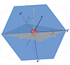 |
Fig. 1. Schematic diagram illustrating the FoMo method for connecting the two grids: the original simulation grid (x, y, z) (gray in the diagram) and the grid (x′,y′,z′) in the observation reference frame (blue in in the diagram). Angle l is around the z-axis and angle b is around the y-axis. The gray and blue planes correspond to the planes perpendicular to the LoS, when it coincides with the z- and z′-axis, respectively. z*-axis in the diagram represents the rotation around y. The red sphere represents the Sun at the center of the coordinate grid. |
2.2. Thomson scattering formulae
In this section, we briefly describe the employed calculations of the radiant intensity in the framework of Thomson scattering theory for white light (Minnaert 1930; Van de Hulst 1950; Billings 1966; Vourlidas & Howard 2006; Howard & Tappin 2009; Howard & DeForest 2012; Inhester 2016).
We assumed the centre of the coordinate system at the Sun’s centre. We considered a radial vector from the centre to the scattering site. Then, the scattering angle, χ, defines the angle between this radial direction and the direction in which the scattered light is observed. The radiant intensity scattered from a single electron can be written as
![Mathematical equation: $$ \begin{aligned} I_{\rm tan}=L \frac{\pi r_{\rm e}^2}{2} [(1-u)C+uD] \end{aligned} $$](/articles/aa/full_html/2025/09/aa54284-25/aa54284-25-eq1.gif) (1)
(1)
and
![Mathematical equation: $$ \begin{aligned} I_{\rm rad}=L \frac{\pi r_{\rm e}^2}{2} [((1-u)C+uD)-((1-u)A+uB)\cdot \sin ^{2}\chi ], \end{aligned} $$](/articles/aa/full_html/2025/09/aa54284-25/aa54284-25-eq2.gif) (2)
(2)
for the tangential and radial components.
Here, the symbol representations are as follows. The parameter u corresponds to the limb darkening coefficient. Generally, it depends on the wavelength and for optical wavelength range was empirically found to be around 0.6 (for ∼5500 Å). Thus, by default, in our calculation routines u = 0.6, but it is an input parameter and can be changed to account for the coronagraph bandpass. The mean radiance over the solar disc L = L⊙(1 − u/3)−1 (Minnaert 1930; Billings 1966), where L⊙ stands for the central radiance, namely, the radiance from the center of the disc as we observe it in the vertical direction (LoS perpendicular to the surface). Then, A, B, C, and D denote the integrals introduced by Minnaert (1930), while re is the classical radius of the electron and Itan denotes the polarisation perpendicular to the scattering plane and is proportional to the solar irradiance polarised in this direction. On the other hand, Irad measures the polarisation in the scattering plane and is proportional to the local irradiance projected normal to the LoS in the scattering plane.
Usually, the combinations Itan − Irad and Itan + Irad are used to determine the polarised (pB) and total (Btot) brightness, respectively. Thus, considering s as the distance along the LoS from the scattering site to the observer and by multiplying the radiant intensity scattered from each electron with the number of electrons ne(s), integration over the LoS gives:
 (3)
(3)
and
 (4)
(4)
Thus, Equations (1)–(4) are calculated the basis of the FoMo routines.
We note, however, that the total brightness includes the unpolarised F-corona component, where scattering is governed by the interplanetary dust particles, rather than free electrons (Blackwell et al. 1967; Koutchmy & Lamy 1985; Lamy 1974; Mann et al. 2004; Howard et al. 2019). Accounting for this mechanism is beyond the scope of the current implementation. In this paper, we mainly focus on the polarised brightness associated with the K-corona, where Thomson scattering by free electrons dominates. Incorporating the different scattering mechanisms would be a highly beneficial (albeit non-trivial task) and it might be considered in future works.
3. Validation tests
In this section, we demonstrate the results of the validation tests performed for the FoMo white-light tool. We aim to demonstrate that it allows for the accurate reproduction of the lower coronal features and the expected shapes of the brightness curves, particularly regarding the polarised brightness. We aim not just to demonstrate the qualitative resemblance to the observations, but also consider the quantitative results of the forward modelling. Thus, we aim to constrain the synthetic results by the observational and analytical and numerical results, offering some insights into the distribution of the coronal density. At the same time, these forward modelling techniques allow us to bring the observations and the simulations together. It also serves a good validation test for the reconstruction methods.
3.1. Analytical example: spherically symmetric density model
To test the above implementation, we first performed forward modelling with a simple analytical example. Thus, we consider a spherically symmetric density model, based on an empirical formula for density from Saito et al. (1977):
 (5)
(5)
where r is the distance from the centre of the Sun in units of solar radii. Coefficients c1, 2 and d1, 2 are calculated using a minimisation technique; thus, when we are substituting the resulting density into the integral equation for pB (for details, see Van de Hulst 1950; Saito et al. 1977), the measured values are reproduced within 5%.
In Fig. 2, panels a and b show the forward-modelled total and polarised brightness. The FoMo synthetic data is in the mean solar brightness (MSB) units. Panel c compares the computed polarised brightness along the equatorial plane to the model equatorial brightness curves for the K-corona, and the computed total brightness along the equatorial plane to the brightness curves for the F-corona. From panel c, we can observe a good agreement between synthetic and observational profiles for the polarised brightness. The total brightness is not adequately reproduced, since the Thomson scattering is not the primary mechanism as we discussed in the previous section. Thus, we chose to further consider the polarised brightness.
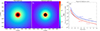 |
Fig. 2. Synthetic images for a spherically symmetric density model, derived in Saito et al. (1977). Panel a: Synthetic total brightness. Panel b: Synthetic polarised brightness. Panel c: Comparison of the computed FoMo total brightness along the equatorial plane (blue line) with the F-corona brightness curve (dark blue dashed line) from Koutchmy & Lamy (1985) and polarised brightness (red line) with the K-corona brightness curve (dotted maroon line) from Saito et al. (1977). |
3.2. Electron density from solar rotational tomography
Secondly, we consider the observation-based 3D electron density to validate the tool further. To this end, we use the recent results (Lloveras et al. 2022) of the solar rotational tomography (SRT, Altschuler & Perry 1972). This is an observational technique that enables a quantitative empirical description of the 3D distribution of fundamental plasma parameters of the solar corona on a global scale, along with the reconstruction of the 3D distribution of the coronal electron density using a time series of white light (WL) coronagraph images that properly constrain all LoSs. The SRT technique has been applied to white light images from coronagraphs such as COR1/SECCHI (e.g. Wang et al. 2017), COR2/SECCHI (e.g. Morgan 2015, 2019), LASCO-C2/SoHO (e.g. Frazin & Janzen 2002; Lamy et al. 2020), and METIS/SolO (e.g. Vásquez et al. 2024). It has also been applied to extreme ultraviolet (EUV) images such as EUVI/STEREO and AIA/SDO (e.g. Frazin et al. 2009; Vásquez et al. 2009; Nuevo et al. 2013; Mac Cormack et al. 2017; Lloveras et al. 2020). In particular, Lloveras et al. (2022) reconstructed the 3D electron density distribution during the solar cycle 24/25 minimum epoch, utilising a modern implementation of SRT developed by Frazin & Janzen (2002). In their work, the authors had already compared the pB images of the LASCO-C2 with the synthetic images calculated from the 3D electron density reconstruction, using the tool developed by Frazin & Janzen (2002). While not all the coronal features were accurately reproduced, this comparison revealed a good agreement between the observation and synthetic images, demonstrating the technique’s capabilities in reconstructing the lower corona electron density. The total uncertainty in the electron density derived from WL-SRT is estimated at 20% (Lloveras et al. 2022), accounting for instrumental (Frazin et al. 2012; Lamy et al. 2020) and reconstruction errors (Lloveras et al. 2022).
In this work, we performed a similar comparison using FoMo white-light tool, with the aim to better qualitatively reproduce the observation. Although we should note that the discussed level of uncertainty with real density values persists and currently appears unavoidable in coronal observations, we demonstrate that the synthetic and the observational pB values are sufficiently close. This supports the idea FoMo might effectively constrain electron density values and contribute to the development of more reliable coronal density models.
We applied the FoMo white-light tool to the 3D density distribution data obtained from WL-SRT tomography during the Whole Heliosphere and Planetary Interactions Campaign Rotation CR-2223 (Lloveras et al. 2022). We then compared our synthetic image to the LASCO-C2 observation (see Fig. 3). The FoMo FoV matches the LASCO FoV exactly in terms of the longitude and latitude of the C2 coronagraph of 6° and 1°, respectively. The plane-of-the-sky resolution is also set to match that of LASCO-C2 – 1024 × 1024 pixels. In panel a of Fig. 3, we show the LASCO-C2 pB image obtained on 16 Oct. 2019. In panel b of Fig. 3, we show the synthetic pB image. The white circle at the origin represents the Sun, and we consider the region between 2.5 and 6.0 R⊙, for which the density reconstruction was performed. We see a good agreement between the real observation and the synthetic image when all the features are well reproduced. For a more detailed comparison, we also considered the radial and latitudinal profiles of pB. The position angle (PA) of 0° corresponds to the Sun’s north and increases anti-clockwise. Panel c shows the pB latitudinal profiles taken at 4.0 R⊙. Panel d shows the pB equatorial radial profiles at the western limb at PA = 270°.
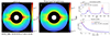 |
Fig. 3. Comparison between the real observational data and synthetic image. Panel a: LASCO C2 observation on 16 October 2019. Panel b: Synthetic image produced with the reconstructed coronal density when the FoV and observation angle match exactly the ones of LASCO C2. Panels c and d: Comparison of the latitudinal and the radial profiles of pB for images in panels a and b. |
4. Coupling with COCONUT
FoMo is easily coupled with state-of-the-art numerical codes, when we can produce the synthetic images and videos simply by reading in the simulation data and setting user parameters (discussed in Section 2 of this paper). This is particularly relevant for the simulations performed on an unstructured grid using the Visualization Toolkit (VTK) file format and files, produced by the cfMesh tool native to COOLFluiD (Lani et al. 2013). In this section, we illustrate the coupling of FoMo with COCONUT, a state-of-the-art code for global solar coronal modelling. For a detailed description of COCONUT, we refer to Perri et al. (2022) and Kuźma et al. (2023).
The present work considers the 3D full MHD simulation of a CME propagation. The CME model is a modified Titov-Démoulin flux rope, developed in Titov & Démoulin (1999), Titov et al. (2014). The CME is launched from the solar surface into the corona. For the details of the model and the CME injection method, we refer to Linan et al. (2023). The mesh used in the code is a sixth-level subdivision of the geodesic polyhedron with 1.5 million cells. More details about the grid and its effects in COCONUT are presented in Brchnelova et al. (2022).
In panel a of Fig. 4, we show the simulation snapshot of the logarithmic scaled density in the xy-plane 36 minutes after launching the CME. Using this simulation, we produced white-light images. We considered the FoV as an area below 8 R⊙ (shown as a white line in panel a) and calculated the polarised brightness for different observational angles. In panel b, we show the synthetic image (left) for b = l = 0, when the scattering plane coincides with the xy-plane. We also show the difference image (right), when we subtract the synthetic data before the ejection of the CME. In panel c, we show the corresponding images for b = 45°, l = 30°. The animation of Fig. 4, for Δt = 70 minutes, is available online.
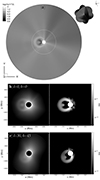 |
Fig. 4. Application of the FoMo white-light tool on a COCONUT simulation of CME propagation. Panel a: Simulation snapshot of the logarithmic density. Panels b and c: Synthetic data for different observational angles. The associated movie is available online. |
We provide a brief overview of FoMo’s time efficiency based on a snapshot of the above 3D simulation. We compare the computation times required when we utilise eight processing cores to process three different spatial resolutions: 512 × 512 pixels, 1024 × 1024 pixels, and 2048 × 2048 pixels. The results are summarised in Table 1. The resolution along the LoS is 200 pixels, which is governed by the original simulation mesh resolution. The increase of the resolution along the LoS results in decreasing tool speed by the factor roughly equal to the factor of the increase. This could stand as a limitation in cases of very-high-resolution numerical simulations employing the adaptive mesh refinements protocols. To capture the finest details of such simulations without sacrificing speed, the FoMo tool might be improved by introducing the protocol with a dynamically sampled LoS, such as that developed by Poirier et al. (2023) for the WindPredict/PLUTO model (Parenti et al. 2022; Réville et al. 2022).
Computation time (on an eight-core processor) for a range of resolutions.
We consider this a proof-of-concept study that effectively demonstrates the capabilities of the FoMo white-light tool. We observe a qualitative resemblance with typical observations of CMEs. The detailed comparison to the observations requires a more realistic model of the CME, which would implement the realistic solar wind and the correct magnetic and thermodynamic properties of the solar corona for a particular event. To this end, FoMo is a valuable tool for validating such a model. We can directly compare the simulation results to the multi-spacecraft observations and perform a case study to perfect the reconstruction of a CME propagation. We can conclude our tool is sufficiently fast and allows for the efficient generation of synthetic videos from the database of the simulation snapshots. This enables studies of the dynamics of a CME by producing synthetic videos of high cadence, offering prospects for a future study.
5. Coupling with MPI-AMRVAC
5.1. Application of the white-light tool on MPI-AMRVAC simulation of the helmet streamer
In this section, we illustrate FoMo usage with the MPI-AMRVAC (Keppens et al. 2012; Porth et al. 2014; Xia et al. 2018). We consider the helmet streamer model in the 2.5D MHD framework. The simulation is performed on a stretched grid with two additional levels of refinement, employed to resolve the streamer. A detailed description of this model is provided by Sorokina et al. (2024), where a parameter study of the streamer’s dynamics was performed. The results of this study were compared to the database of streamer wave events, observed from three different coronagraphs: LASCO-C2 (Brueckner et al. 1995), and STEREO COR2 A, and STEREO COR2 B (Kaiser et al. 2008).
First, using the white-light tool, we produced the synthetic data of a particular modelling event ‘B2T1.50’ (see Fig. 3 in Sorokina et al. 2024) before the triggering of a streamer wave, namely, the outwardly propagating oscillation of the streamer stalk (Chen et al. 2010; Feng et al. 2011). Generally, FoMo allows the generation of synthetic data from a 2D simulation snapshot. The result of such a calculation can be seen in Fig. 5, where we show a simulation snapshot of the logarithmic density and the polarised brightness, calculated directly from this simulation snapshot.
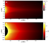 |
Fig. 5. Application of the FoMo white-light tool on an MPI-AMRVAC simulation of a helmet streamer. Panel a: Simulation snapshot of the logarithmic density, depicting the streamer model ‘B2T1.50’ from Sorokina et al. (2024). Panel b: Polarised brightness, calculated directly from this simulation snapshot. Here, the dark circle represents a patch to mask the distance below 1.5 R⊙. |
To consider a more realistic scenario, we also produced a new pseudo-3D dataset by assuming axisymmetry and revolving the calculated in simulation 2D density scalar field around the z-axis. Based on the observational study by Decraemer et al. (2019), we assumed the 3D structure of the steamer as a fan of an angular width of several degrees when observed face-on. We considered two types of snapshots of the solar corona: with and without the presence of the helmet streamer. We considered a half-cylinder with Sun at the origin, where ρ ∈ [1 R⊙, 14 R⊙], ϕ ∈ [ − 90° ,90° ] and z ∈ [ − 3 R⊙, 3 R⊙], containing the ‘streamer’ snapshots for ϕ ∈ [ − 20° ,20° ] (see Fig. 6).
 |
Fig. 6. Pseudo-3D cylindrical dataset construction scheme. |
This paper is aimed at comparing the synthetic data produced from the aforementioned 3D data cube to the observations studied in Decraemer et al. (2019). The authors considered a streamer structure, observed simultaneously from LASCO-C2 and COR2 aboard STEREO A on 30 April 2011. The view from COR2 showed a narrow streamer stalk viewed edge-on (see Fig. 7, panel d; the real observation is rotated to align the streamer axis with the horizontal axis). The separation angle between STEREO A and SOHO was very close to 90°. Thus, the view from C2 was considered to be the face-on view (see panel e in Fig. 7). To determine the position and geometry of the streamer in 3D space Decraemer et al. (2019) considered the STEREO/COR2 A synoptic map (Wang et al. 2000; Zhukov et al. 2008) and the potential field source surface (PFSS) map of the extrapolated coronal magnetic field from the Wilcox Solar Observatory (WSO; Scherrer et al. 1977) photospheric magnetogram. The authors thus approximated the 3D configuration of the helmet streamer by a slab-like structure, with an angular extent of 40° in the Carrington longitude. In the face-on view, it is centred around the central axis (see cyan dashed line in panel e of Fig. 7).
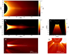 |
Fig. 7. Comparison between the synthetic and observational data. Panel a: Calculation of the pB from the 3D cylindrical dataset. Panels b and c: Background-subtracted images of the calculated synthetic data for FoVs corresponding to the streamer observations edge-on and face-on, respectively. Panels d and e: Observations on 30 April 2011 from STEREO COR2-A and LASCO C2, respectively. Here, the dark circle represents a patch to mask the distance below 2.0 R⊙. |
We performed the forward modelling for two LoS and two FoVs, which correspond to a streamer observed edge-on and face-on by STEREO COR2-A and LASCO C2, respectively. The synthetic imaging results for the discussed density cube are presented in Fig. 7. Panel a shows the synthetic image generated from the 3D cylindrical dataset of a streamer. To highlight the streamer structure in panels b and c, we show the difference images for the two FoVs, where we subtracted the synthetic data for a fully ‘non-streamer’ data cube. In panel d, we show STEREO COR2-A observation of the streamer edge-on 30 Apr. 2011 at 16:24:00. In panel e, we show the LASCO C2 observation of the same feature face-on on 30 April 2011 at 16:24:05. The resolutions for all of the described synthetic images are also set to match one of COR2-A and C2 at 1024 × 1024 pixels. The resolution along the LoS was set to 1000 pixels.
For a more detailed comparison, we also considered the pB profiles along the radial (along the streamer; see the blue line in panel b and cyan line in panel d) and arc-shaped (across the streamer, seen in the blue line in panel c and cyan line in panel e) lines for STEREO COR2-A and LASCO C2 observations. In Fig. 8, we compare this observational data and pB calculated by the FoMo white-light tool. We consider polarised brightness profiles along the radial line aligned with the streamer axis and along the arc-shaped line at 3 R⊙.
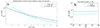 |
Fig. 8. Comparison between the synthetic and observational data. Panel a: Equatorial radial profiles of the synthetic and observational pB data along the horizontal slits (from panels b and d in Fig. 7). Panel b: Latitudinal profiles of the synthetic and observational pB data along the arc-shaped slits (shown in panels c and e in Fig. 7). |
Overall, we observe a good agreement between the observations and forward modelling results. Thus, we can conclude our model is equipped to qualitatively represent the streamer structure and its properties. We can also gain information on improving our numerical model by comparing the synthetic and observational data. For instance, the density model in the discussed MPI-AMRVAC simulation decreases, such as r−2. Furthermore, in panel a of Fig. 8, we observe the difference in the shape of the pB radial profiles between the modelling and observations. To eliminate this discrepancy, we can try to improve our simulation by considering a more realistic density distribution, estimated from the observations.
5.2. Application of the white-light tool on MPI-AMRVAC simulation of the streamer wave
We also consider a model of a streamer wave propagation constructed in Sorokina et al. (2024) of the event ‘B2T1.50’ (discussed in the previous section). In Fig. 9, we compare the synthetic images obtained from the streamer wave MHD simulation with STEREO COR2-A observation of the streamer wave phenomena on 2013 Feb. 6, identified in Decraemer et al. (2020). Panel a shows the STEREO A/COR2 white-light image of the streamer wave event 13 from Decraemer et al. (2020) identified on 6 Feb. 2013 from 00:24:00 to 06:24:00, at 02:39:00 (∼2 hours after the start of the event) cropped to match the forward modelling data snapshots. Panel b shows the FoMo pB image of the modelling event from Sorokina et al. (2024) at three hours after the introduction of the perturbation, depicting the streamer’s outward-propagating transverse oscillations. The videos of the streamer wave events are available online.
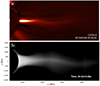 |
Fig. 9. Comparison of the forward modelling results with the observations. Panel a: STEREO A/COR2 white-light image of the streamer wave event on 6 February 2013. Panels b: Synthetic snapshot of the streamer wave propagation, obtained from the density data-cube based on the MHD simulation of the streamer wave phenomena. Here, the dark circle represents a patch to mask the distance below 2.0 R⊙. The associated movie is available online. |
Forward modelling could allow for a more thorough analysis of solar phenomena. We considered streamer wave dynamics, evaluated from white-light synthetic data from the 3D simulation data-cubes, discussed in the previous section. We made a comparison to the 2.5D MHD simulation results from Sorokina et al. (2024). After applying the forward modelling technique on the event ‘B2T1.50’, we measured the key properties of the streamer wave, such as wavelength, period, and phase speed, in the inertial frame of reference. We treated the synthetic data with the same methodology applied to the STEREO A/COR2 observations in Decraemer et al. (2020).
To measure the wavelength, we considered the running-difference images at 03:00:00, 04:00:00, 05:00:00 and 06:00:00, where 00:00:00 corresponds to the start of the wave event, shown in panels a–d of Fig. 10. We outlined the wavelength from each image and take the average of these four measurements, indicated by the green lines. To measure the period, we constructed a time–distance map along the slit with a width of 0.1 R⊙, located at 12 R⊙ (see the green line in panel b in Fig. 9). We then measured the half-period as the time between the trough and the crest, as shown in panel e of Fig. 10. After introducing the perturbation, we took snapshots of the original simulation every 12 minutes. We considered the cadence of the virtual spacecraft to be 12 minutes, with a reference to the COR2 instrument’s cadence of 15 minutes. To measure the phase speed of the streamer wave in the inertial frame of reference, we tracked the height of the extrema of the wave. The measurements are indicated in the images in panels a–d and also shown in the plot in panel f as green dots. We then fit a linear profile to these points, which we used to determine the measured phase speed of the wave. We also estimated the proper phase speed of the mode using the simple formula λ/P.
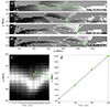 |
Fig. 10. Panels a–d: Running difference images of the streamer wave event at 03:00:00, 04:00:00, 05:00:00, and 06:00:00 (where 00:00:00 corresponds to the introduction of the perturbation). The green line in panel a shows how we performed the wavelength measurements (λ = 7.5 R⊙). Panel e: Time–distance map along the slit, shown in panel b in Fig. 9. The green line in panel e indicates the half-period measurement (P/2 = 156 min). Panel f: Height–time plot, where the dots correspond to the streamer wave extrema at four times, indicated in panels a-d. The linear fit indicates the measured phase speed (vph = 491 km/s). |
In Fig. 11, we compare the MHD numerical results for the discussed modelling event ‘B2T1.50’ from Sorokina et al. (2024) to its forward modelling results. In panel a, we can observe a similar trend as in observational and numerical studies, when the more extended periods correspond to bigger wavelengths. In panel b, we show the relation between the calculated and the measured phase speeds. The red line corresponds to the equal values of the quantities. In accordance with the observations and numerical results, we observed the Doppler shift in the MHD wave theory, where the measured phase speed has two contributions: the proper phase speed of the wave and the background solar wind speed. The dotted line corresponds to a forward-propagating wave and a simple fit, λ/P = vph − vSW, found in the observational study (Decraemer et al. 2020). Overall, we observe a considerable change in the phase speeds, namely, when the synthetic data better corresponds to the linear fit. The discrepancy between the observational and numerical study, found in Sorokina et al. (2024), could thus be at least partially eliminated by assuming the fan-like 3D streamer structure and considering the synthetic data. If we compare the projected and de-projected values of the measured phase speed for this event, the difference is around 20%. This highlights the importance of carefully considering projection effects when interpreting observational phase speeds and supports the need for forward modelling to enable more direct comparisons between the numerical results and observations.
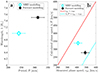 |
Fig. 11. Comparison between the numerical simulation and forward modelling results for the streamer wave event ‘B2T1.50’. Panel a: Period vs. wavelength. Panel b: Measured phase speed (vph) vs calculated speed (λ/P). The red line corresponds to the equal values of the quantities. The dotted line corresponds to a fit λ/P = vph − vSW. |
6. Conclusions
The FoMo code was extended by introducing a new white-light package, which utilises Thomson scattering theory to generate synthetic data. This tool can operate in popular data formats with density data cubes and simulation snapshots. FoMo is coupled with advanced numerical tools, such as MPI-AMRVAC and COCONUT, and allows for the production of white-light data in a fast and user-friendly way. We also believe the white-light tool can be adapted for a wide range of simulations, allowing an efficient generation of synthetic images and videos.
The white-light tool was validated by considering data cubes, obtained from an empirical formula of the coronal density and from the recent results from the WL-SRT observational technique. We illustrated using the FoMo white-light package by applying it directly to the snapshots of the 3D COCONUT modelling of CME propagation and 2.5D ARMVAC modelling of streamer waves. We also performed a thorough analysis of the streamer wave event modelling. We demonstrated that the synthetic data produced by FoMo aligns well with the results of the multi-spacecraft streamer wave observational study. Our findings highlight the importance of carefully considering projection effects when interpreting observations and indicate that incorporating synthetic data can reduce the discrepancies between observational and numerical studies of the streamer wave dynamics.
Overall, forward modelling fills the gap between observational data and numerical models. It can help us interpret observations, improve numerical models, and gain insight into coronal plasma parameters. Further developments of the tool could include several potential improvements. For instance, we could consider different scattering mechanisms to account for the F-corona component. Potentially, FoMo might be improved by introducing the adaptive mechanism for the LoS sampling to capture the finest details of high-resolution numerical simulations without sacrificing tool speed. Currently, the virtual spacecraft FOV and positioning are defined manually by the user. It would be useful to develop an interface that allows automatic alignment the coordinates of the simulations and observations, for instance, by working with standardised systems, such as Earth’s ecliptic and heliographic coordinates. This would be particularly useful for fast-moving spacecraft, such as SolO and PSP. These are prospects for a future study.
Data availability
Movies associated to Figs. 4 and 9 are available at https://www.aanda.org
The data that support the findings of this study are openly available in GitHub: FoMo at https://github.com/TomVeeDee/FoMo
Acknowledgments
The STEREO/SECCHI data used here are produced by an international consortium of the Naval Research Laboratory (USA), Lockheed Martin Solar and Astrophysics Laboratory (USA), NASA Goddard Space Flight Center (USA), Rutherford Appleton Laboratory (UK), University of Birmingham (UK), Max-Planck-Institut für Sonnensystemforschung (Germany), Centre Spatial de Liège (Belgium), Institut d’Optique Théorique et Appliqué (France), and Institut d’Astrophysique Spatiale (France). This work makes use of the LASCO-C2 legacy archive data produced by the LASCO-C2 team at the Laboratoire d’Astrophysique de Marseille and the Laboratoire Atmosphères, Milieux, Observations Spatiales, both funded by the Centre National d’Etudes Spatiales (CNES). LASCO was built by a consortium of the Naval Research Laboratory, USA, the Laboratoire d’Astrophysique de Marseille (formerly Laboratoire d’Astronomie Spatiale), France, the Max-Planck-Institut für Sonnensystemforschung (formerly Max Planck Institute für Aeronomie), Germany, and the School of Physics and Astronomy, University of Birmingham, UK. SOHO is a project of international cooperation between ESA and NASA. For the computations in the present work, we used the infrastructure of the VSC “Flemish Supercomputer Center, funded by the Hercules Foundation and the Flemish Government” department EWI. TVD was supported by the European Research Council (ERC) under the European Union’s Horizon 2020 research and innovation programme (grant agreement No 724326), the C1 grant TRACEspace of Internal Funds KU Leuven, and a Senior Research Project (G088021N) of the FWO Vlaanderen. Furthermore, TVD received financial support from the Flemish Government under the long-term structural Methusalem funding program, project SOUL: Stellar evolution in full glory, grant METH/24/012 at KU Leuven. The research that led to these results was subsidised by the Belgian Federal Science Policy Office through the contract B2/223/P1/CLOSE-UP. This work is also part of the DynaSun project and has thus received funding under the Horizon Europe programme of the European Union under grant agreement (no. 101131534). Views and opinions expressed are however those of the author(s) only and do not necessarily reflect those of the European Union and therefore the European Union cannot be held responsible for them. SP was supported by the projects C16/24/010 C1 project Internal Funds KU Leuven, G0B5823N and G002523N (WEAVE) (FWO-Vlaanderen), and 4000145223 (SIDC Data Exploitation (SIDEX2), ESA Prodex).
References
- Altschuler, M. D., & Perry, R. M. 1972, Sol. Phys., 23, 410 [Google Scholar]
- Antonucci, E., Romoli, M., Andretta, V., et al. 2020, A&A, 642, A10 [NASA ADS] [CrossRef] [EDP Sciences] [Google Scholar]
- Billings, D. E. 1966, A Guide to the Solar Corona (New York: Academic Press) [Google Scholar]
- Blackwell, D. E., Dewhirst, D. W., & Ingham, M. F. 1967, Adv. Astron. Astrophys., 5, 1 [Google Scholar]
- Brchnelova, M., Zhang, F., Leitner, P., et al. 2022, J. Plasma Phys., 88, 905880205 [NASA ADS] [CrossRef] [Google Scholar]
- Brueckner, G. E., Howard, R. A., Koomen, M. J., et al. 1995, Sol. Phys., 162, 357 [NASA ADS] [CrossRef] [Google Scholar]
- Cécere, M., Costa, A., & Van Doorsselaere, T. 2023, A&A, 676, A8 [NASA ADS] [CrossRef] [EDP Sciences] [Google Scholar]
- Chen, Y., Song, H. Q., Li, B., et al. 2010, ApJ, 714, 644 [NASA ADS] [CrossRef] [Google Scholar]
- Decraemer, B., Zhukov, A., & Van Doorsselaere, T. 2019, ApJ, 883, 152 [NASA ADS] [CrossRef] [Google Scholar]
- Decraemer, B., Zhukov, A., & Van Doorsselaere, T. 2020, ApJ, 893, 78 [NASA ADS] [CrossRef] [Google Scholar]
- Deforest, C., Killough, R., Gibson, S., et al. 2022, IEEE Aerospace Conf., 1, 1 [Google Scholar]
- Feng, S. W., Chen, Y., Li, B., et al. 2011, Sol. Phys., 272, 119 [NASA ADS] [CrossRef] [Google Scholar]
- Frazin, R. A., & Janzen, P. 2002, ApJ, 570, 408 [Google Scholar]
- Frazin, R. A., Vásquez, A. M., & Kamalabadi, F. 2009, ApJ, 701, 547 [Google Scholar]
- Frazin, R. A., Vásquez, A. M., Thompson, W. T., et al. 2012, Sol. Phys., 280, 273 [NASA ADS] [CrossRef] [Google Scholar]
- Gibson, S., Kucera, T., White, S. M., et al. 2016, Front. Astron. Space Sci., 3, 8 [NASA ADS] [CrossRef] [Google Scholar]
- Guo, M., Gao, Y., Van Doorsselaere, T., & Goossens, M. 2023, A&A, 676, L7 [NASA ADS] [CrossRef] [EDP Sciences] [Google Scholar]
- Howard, R. A., & DeForest, C. E. 2012, ApJ, 752, 130 [Google Scholar]
- Howard, R. A., & Tappin, S. J. 2009, Space Sci. Rev., 147, 31 [NASA ADS] [CrossRef] [Google Scholar]
- Howard, R. A., Vourlidas, A., Bothmer, V., et al. 2019, Nature, 576, 232 [Google Scholar]
- Inhester, B. 2016, ArXiv e-prints [arXiv:1512.00651] [Google Scholar]
- Kaiser, M. L., Kucera, T. A., Davila, J. M., et al. 2008, Space Sci. Rev., 136, 5 [Google Scholar]
- Keppens, R., Meliani, Z., van Marle, A., et al. 2012, J. Comput. Phys., 231, 718 [Google Scholar]
- Koutchmy, S., & Lamy, P. L. 1985, Properties and Interactions of Interplanetary Dust (Dordrecht: Reidel) [Google Scholar]
- Kuźma, B., Brchnelova, M., Perri, B., et al. 2023, Am. Astron. Soc., 942, 31 [Google Scholar]
- Lamy, P. L. 1974, A&A, 33, 191 [Google Scholar]
- Lamy, P., Llebaria, A., Boclet, B., et al. 2020, Sol. Phys., 295, 89 [CrossRef] [Google Scholar]
- Lani, A., Villedieu, N., Bensassi, K., et al. 2013, 21st AIAA Computational Fluid Dynamics Conference, 2589 [Google Scholar]
- Liewer, P., Vourlidas, A., Thernisien, A., et al. 2019, Sol. Phys., 294, 93 [Google Scholar]
- Linan, L., Regnault, F., Perri, B., et al. 2023, A&A, 675, A101 [NASA ADS] [CrossRef] [EDP Sciences] [Google Scholar]
- Lloveras, D., Vásquez, A. M., Nuevo, F. A., et al. 2020, Sol. Phys., 295, 76 [Google Scholar]
- Lloveras, D., Vásquez, A. M., Nuevo, F. A., et al. 2022, J. Geophys. Res.: Space Phys., 127, e30406 [Google Scholar]
- Mac Cormack, C., Vásquez, A. M., López Fuentes, M., et al. 2017, ApJ, 843, 70 [NASA ADS] [CrossRef] [Google Scholar]
- Mann, I., Kimura, H., Biesecker, D. A., et al. 2004, Space Sci. Rev., 110, 269 [Google Scholar]
- Minnaert, M. 1930, Z. Astrophys., 1, 209 [NASA ADS] [Google Scholar]
- Morgan, H. 2015, ApJS, 219, 23 [CrossRef] [Google Scholar]
- Morgan, H. 2019, ApJS, 242, 3 [NASA ADS] [CrossRef] [Google Scholar]
- Nuevo, F. A., Huang, Z., Frazin, R., et al. 2013, ApJ, 773, 9 [Google Scholar]
- Parenti, S., Réville, V., Brun, A. S., et al. 2022, ApJ, 929, 75 [NASA ADS] [CrossRef] [Google Scholar]
- Perri, B., Leitner, P., Brchnelova, M., et al. 2022, ApJ, 936, 23 [NASA ADS] [CrossRef] [Google Scholar]
- Pinto, R. F., & Rouillard, A. P. 2017, ApJ, 838, 89 [NASA ADS] [CrossRef] [Google Scholar]
- Poirier, N., Kouloumvakos, A., Rouillard, A. P., et al. 2020, ApJS, 246, 60 [Google Scholar]
- Poirier, N., Réville, V., Rouillard, A. P., Kouloumvakos, A., & Valette, E. 2023, A&A, 677, A108 [NASA ADS] [CrossRef] [EDP Sciences] [Google Scholar]
- Porth, O., Xia, C., Hendrix, T., Moschou, S. P., & Keppens, R. 2014, ApJS, 214, 4 [Google Scholar]
- Réville, V., Fargette, N., Rouillard, A. P., et al. 2022, A&A, 659, A110 [CrossRef] [EDP Sciences] [Google Scholar]
- Reznikova, V. E., Antolin, P., & Van Doorsselaere, T. 2014, ApJ, 785, 86 [NASA ADS] [CrossRef] [Google Scholar]
- Sachdeva, N., van der Holst, B., Manchester, W. B., et al. 2019, ApJ, 887, 83 [NASA ADS] [CrossRef] [Google Scholar]
- Saito, K., Poland, A. I., & Munro, R. H. 1977, Sol. Phys., 55, 121S [Google Scholar]
- Scherrer, P. H., Wilcox, J. M., Svalgaard, L., et al. 1977, Sol. Phys., 54, 353 [NASA ADS] [CrossRef] [Google Scholar]
- Sorokina, D., Van Doorsselaere, T., Talpeanu, D.-C., & Poedts, S. 2024, A&A, 682, A168 [NASA ADS] [CrossRef] [EDP Sciences] [Google Scholar]
- Thernisien, A. F., & Howard, R. A. 2006, ApJ, 642, 523 [Google Scholar]
- Thernisien, A., Vourlidas, A., & Howard, R. A. 2011, J. Atmos. Sol. Terr. Phys., 73, 1156 [Google Scholar]
- Titov, V. S., & Démoulin, P. 1999, A&A, 351, 707 [NASA ADS] [Google Scholar]
- Titov, V. S., Török, T., Mikic, Z., & Linker, J. A. 2014, ApJ, 790, 163 [NASA ADS] [CrossRef] [Google Scholar]
- Török, T., Downs, C., Linker, J. A., et al. 2018, ApJ, 856, 75 [Google Scholar]
- Van de Hulst, H. C. 1950, Bull. Astron. Inst. Neth., 11, 135 [Google Scholar]
- Van Doorsselaere, T., Antolin, P., Yuan, D., Reznikova, V., & Magyar, N. 2016, Front. Astron. Space Sci., 3, 4 [Google Scholar]
- Vásquez, A. M., Frazin, R. A., & Kamalabadi, F. 2009, Sol. Phys., 256, 73 [Google Scholar]
- Vásquez, A. M., Nuevo, F. A., Romoli, M., et al. 2024, Sol. Phys., 299, 165 [Google Scholar]
- Vourlidas, A., & Howard, R. A. 2006, ApJ, 642, 1216 [Google Scholar]
- Vourlidas, A., Howard, R. A., Plunkett, S. P., et al. 2016, Space Sci. Rev., 204, 83 [Google Scholar]
- Wang, Y. M., Sheeley, N. R., & Rich, N. B. 2000, Geophys. Res. Lett., 27, 149 [NASA ADS] [CrossRef] [Google Scholar]
- Wang, T., Reginald, N. L., Davila, J. M., et al. 2017, Sol. Phys., 292, 97 [Google Scholar]
- Wang, T., Arge, C. N., & Jones, S. I. 2025, Sol. Phys., 300, 46 [Google Scholar]
- Xia, C., Teunissen, J., Mellah, I. E., Chané, E., & Keppens, R. 2018, ApJS, 234, 30 [NASA ADS] [CrossRef] [Google Scholar]
- Zhukov, A. N., Saez, F., Lamy, P., Llebaria, A., & Stenborg, G. 2008, ApJ, 680, 1532 [NASA ADS] [CrossRef] [Google Scholar]
All Tables
All Figures
|
Fig. 1. Schematic diagram illustrating the FoMo method for connecting the two grids: the original simulation grid (x, y, z) (gray in the diagram) and the grid (x′,y′,z′) in the observation reference frame (blue in in the diagram). Angle l is around the z-axis and angle b is around the y-axis. The gray and blue planes correspond to the planes perpendicular to the LoS, when it coincides with the z- and z′-axis, respectively. z*-axis in the diagram represents the rotation around y. The red sphere represents the Sun at the center of the coordinate grid. |
| In the text | |
|
Fig. 2. Synthetic images for a spherically symmetric density model, derived in Saito et al. (1977). Panel a: Synthetic total brightness. Panel b: Synthetic polarised brightness. Panel c: Comparison of the computed FoMo total brightness along the equatorial plane (blue line) with the F-corona brightness curve (dark blue dashed line) from Koutchmy & Lamy (1985) and polarised brightness (red line) with the K-corona brightness curve (dotted maroon line) from Saito et al. (1977). |
| In the text | |
|
Fig. 3. Comparison between the real observational data and synthetic image. Panel a: LASCO C2 observation on 16 October 2019. Panel b: Synthetic image produced with the reconstructed coronal density when the FoV and observation angle match exactly the ones of LASCO C2. Panels c and d: Comparison of the latitudinal and the radial profiles of pB for images in panels a and b. |
| In the text | |
|
Fig. 4. Application of the FoMo white-light tool on a COCONUT simulation of CME propagation. Panel a: Simulation snapshot of the logarithmic density. Panels b and c: Synthetic data for different observational angles. The associated movie is available online. |
| In the text | |
|
Fig. 5. Application of the FoMo white-light tool on an MPI-AMRVAC simulation of a helmet streamer. Panel a: Simulation snapshot of the logarithmic density, depicting the streamer model ‘B2T1.50’ from Sorokina et al. (2024). Panel b: Polarised brightness, calculated directly from this simulation snapshot. Here, the dark circle represents a patch to mask the distance below 1.5 R⊙. |
| In the text | |
|
Fig. 6. Pseudo-3D cylindrical dataset construction scheme. |
| In the text | |
|
Fig. 7. Comparison between the synthetic and observational data. Panel a: Calculation of the pB from the 3D cylindrical dataset. Panels b and c: Background-subtracted images of the calculated synthetic data for FoVs corresponding to the streamer observations edge-on and face-on, respectively. Panels d and e: Observations on 30 April 2011 from STEREO COR2-A and LASCO C2, respectively. Here, the dark circle represents a patch to mask the distance below 2.0 R⊙. |
| In the text | |
|
Fig. 8. Comparison between the synthetic and observational data. Panel a: Equatorial radial profiles of the synthetic and observational pB data along the horizontal slits (from panels b and d in Fig. 7). Panel b: Latitudinal profiles of the synthetic and observational pB data along the arc-shaped slits (shown in panels c and e in Fig. 7). |
| In the text | |
|
Fig. 9. Comparison of the forward modelling results with the observations. Panel a: STEREO A/COR2 white-light image of the streamer wave event on 6 February 2013. Panels b: Synthetic snapshot of the streamer wave propagation, obtained from the density data-cube based on the MHD simulation of the streamer wave phenomena. Here, the dark circle represents a patch to mask the distance below 2.0 R⊙. The associated movie is available online. |
| In the text | |
|
Fig. 10. Panels a–d: Running difference images of the streamer wave event at 03:00:00, 04:00:00, 05:00:00, and 06:00:00 (where 00:00:00 corresponds to the introduction of the perturbation). The green line in panel a shows how we performed the wavelength measurements (λ = 7.5 R⊙). Panel e: Time–distance map along the slit, shown in panel b in Fig. 9. The green line in panel e indicates the half-period measurement (P/2 = 156 min). Panel f: Height–time plot, where the dots correspond to the streamer wave extrema at four times, indicated in panels a-d. The linear fit indicates the measured phase speed (vph = 491 km/s). |
| In the text | |
|
Fig. 11. Comparison between the numerical simulation and forward modelling results for the streamer wave event ‘B2T1.50’. Panel a: Period vs. wavelength. Panel b: Measured phase speed (vph) vs calculated speed (λ/P). The red line corresponds to the equal values of the quantities. The dotted line corresponds to a fit λ/P = vph − vSW. |
| In the text | |
Current usage metrics show cumulative count of Article Views (full-text article views including HTML views, PDF and ePub downloads, according to the available data) and Abstracts Views on Vision4Press platform.
Data correspond to usage on the plateform after 2015. The current usage metrics is available 48-96 hours after online publication and is updated daily on week days.
Initial download of the metrics may take a while.