| Issue |
A&A
Volume 701, September 2025
|
|
|---|---|---|
| Article Number | A271 | |
| Number of page(s) | 16 | |
| Section | Extragalactic astronomy | |
| DOI | https://doi.org/10.1051/0004-6361/202554528 | |
| Published online | 22 September 2025 | |
Through the fog: A complementary optical galaxy classification scheme for intermediate redshifts
1
Aix Marseille Univ., CNRS, CNES, LAM, Marseille, France
2
Instituto de Astrofísica e Ciências do Espaço, Universidade de Lisboa – OAL, Tapada da Ajuda, PT1349-018 Lisboa, Portugal
3
Departamento de Física, Faculdade de Ciências da Universidade de Lisboa, Edifício C8, Campo Grande, PT1749-016 Lisboa, Portugal
4
Instituto de Astrofísica e Ciências do Espaço, Universidade do Porto – CAUP, Rua das Estrelas, PT4150-762, Porto, Portugal
5
Departamento de Física e Astronomia, Faculdade de Ciências, Universidade do Porto, Rua do Campo Alegre 687, PT4169-007 Porto, Portugal
6
Institute of Astrophysics, Facultad de Ciencias Exactas, Universidad Andrés Bello, Sede Concepción, Talcahuano, Chile
⋆ Corresponding author: This email address is being protected from spambots. You need JavaScript enabled to view it.
Received:
14
March
2025
Accepted:
23
July
2025
Abstract
Context. Understanding the evolution of galaxies strongly depends on our interpretation of their spectra. In the optical, BPT diagrams have been the main way to distinguish whether the principal excitation mechanism of a galaxy is dominated by star formation (SF) or by an active galactic nucleus (AGN). Although different classification methods exist, they are based on either hard-to-detect or high-energy emission lines. To date, the Balmer lines remain the most consistent way to classify galaxies, but at intermediate redshifts (1.5 < z < 2.5), galaxies are hard to parse in the BPT diagrams (and siblings) because the crucial Hα emission line is out of the range of ground-based optical spectrographs.
Aims. In this work, we re-explore a diagram, which we call the OB-I diagram, that compares the equivalent width of Hβ and the emission line flux ratio of [OIII]λ5007/Hβ, and we breathe new life into it as it has the potential to be used for the classification of galaxies at these intermediate redshifts and to ‘clear the fog’ that permeates galaxy classification in the optical rest frame.
Methods. We used data from SDSS, LEGA-C, VANDELS, JADES, 3D-HST, and MOSDEF to explore galaxy classifications in the OB-I diagram across a wide range of redshifts (0 < z < 2.7).
Results. Our results show that, at z < 0.4, the OB-I diagram clearly separates galaxies between two distinct types: one dominated by an AGN and a second made up of a mixed population of SF galaxies and AGN activity. Comparison with the BPT diagrams and theoretical models shows that this mixed population can be partially separated from a pure SF population with a simple semi-empirical fit. At higher redshifts, we find that half of AGNs identified by other classification schemes are correctly recovered by the OB-I diagram, potentially making this diagram resistant to the cosmic shift that plagues most optical classification schemes, but more research is needed to understand this phenomenon.
Conclusions. We find the OB-I diagram, which only requires two emission lines to be implemented, to be a useful tool at separating galaxies that possess a dominating AGN component in their emission from others. This applies not only to the Local Universe, but also seemingly at redshifts near the Cosmic Noon (z ∼ 2), without any need for significant adjustments in our empirical fit.
Key words: methods: numerical / techniques: spectroscopic / galaxies: active / galaxies: evolution / galaxies: star formation / galaxies: statistics
© The Authors 2025
 Open Access article, published by EDP Sciences, under the terms of the Creative Commons Attribution License (https://creativecommons.org/licenses/by/4.0), which permits unrestricted use, distribution, and reproduction in any medium, provided the original work is properly cited.
This article is published in open access under the Subscribe to Open model. This email address is being protected from spambots. You need JavaScript enabled to view it. to support open access publication.
1. Introduction
Galaxies are complex and dynamic systems, and analysing their spectra is one of the best tools we have to better comprehend them. To understand the nature of galaxies, however, there is a need to distinguish whether their principal excitation mechanisms are governed by photoionisation from hot massive stars – directly related with ongoing or recent star-forming (SF) activity (Osterbrock & Ferland 2006) – or by an active galactic nucleus (AGN).
Five decades ago Searle et al. (1972) noticed that line ratios were efficient at separating older and younger spiral galaxies. In the 1980s Baldwin et al. (1981) took advantage of this to create several diagrams that compared the ratio of specific emission lines and were able to separate galaxies according to their main excitation mechanism. Further investigation of these diagrams by Veilleux & Osterbrock (1987) showed that there were three diagrams that performed this efficiently: [NII]λ6584/Hα versus [OIII]λ5007/Hβ; [SII]λλ6717, 6731/Hα versus [OIII]λ5007/Hβ, and [OI]λ6300/Hα versus [OIII]λ5007/Hβ (hereafter the NII, SII, and OI diagrams, respectively). To simplify, galaxies were separated into two clear and distinct types: SF and AGNs.
Nearly 20 years later, thanks to projects like the Sloan Digital Sky Survey (SDSS, Fukugita et al. 1996; Gunn et al. 1998; York et al. 2000) the interpretation of these diagrams was refined. In Kewley et al. (2001), through a combination of stellar population synthesis and photoionisation models, the authors were able to determine the first theoretical maximum starburst line in the NII, SII, and OI diagrams, which determined the location in the parameter space of galaxies whose emission is dominated by star-forming activity. Furthermore, Kauffmann et al. (2003) adjusted a semi-empirical fit to the NII diagram, which allowed for the definition of another class, Composite galaxies, which are galaxies that have a mix of both star formation and AGN activity. This separation between SF and Composite galaxies is due to the fact that the [NII]λ6584/Hα ratio saturates at high metallicities, considering only the nebular contribution (Kewley & Dopita 2002; Denicoló et al. 2002). For galaxies to have higher contributions of the [NII]λ6584 emission line, there must be a mechanism inside the galaxy that boosts the value of its flux, in this case an AGN (Kewley et al. 2006).
The BPT diagrams have been proven time and time again to be a great tool that astrophysicists can use to separate galaxy types, and a countless number of papers have used it to classify galaxies and explore the consequences of these classes (Lagos et al. 2022; Polimera et al. 2022; Harish et al. 2023; Teimoorinia et al. 2024, to cite just a few). However, it is not the only classification scheme available using optical lines. Another relevant example is the WHAN diagram (Cid Fernandes et al. 2011), which takes its name from its use of the equivalent width (EW) of Hα and the flux ratio of Hα and [NII]λ6584. This classification scheme is mostly used to distinguish active galaxies (galaxies that are actively forming stars) from passive ones (galaxies that show no star formation in the present). Instead of Balmer lines, one can base the classification on oxygen or nitrogen lines (Rola et al. 1997; Paalvast et al. 2018; Perrotta et al. 2021). There are also the mass-excitation diagrams (Juneau et al. 2011), which combine the emission lines of galaxies with their physical properties in order to distinguish the effects and degeneracies present in these ratios.
All of these diagrams are useful, but they are mostly applied in the Local Universe (z < 0.1). At higher redshifts, the BPT diagram becomes difficult to interpret, but in the advent of advanced space telescopes such as the James Webb Space Telescope (JWST, Gardner et al. 2006), diagrams that use higher-order emission lines such as the forbidden line ratio (FLR; Feuillet et al. 2024); a comparison between oxygen, hydrogen, and neon lines (OHNO; Backhaus et al. 2022); and high-energy or auroral lines (e.g. HeII/Hβ, Solimano et al. 2025; [OIII]λ4363/Hγ, Mazzolari et al. 2024) can now be plotted for a wide selection of galaxies, thus providing the scientific community with new tools for separating galaxy types and disentangling their properties.
However, there is a great deal of data that does not reside in the realm of detection of space-based instruments such as JWST. The aforementioned SDSS and the Dark Energy Spectroscopic Instrument (DESI, DESI Collaboration 2024) surveys reside in the optical, and in this regime it is not always possible to apply these diagnostics either due to emission lines such as Hα moving out of the range of the spectrographs at higher redshifts (z ≳ 0.5, e.g. BPT diagrams or WHAN diagram) or because higher-order emission lines are very difficult to detect and demand high signal-to-noise ratios (S/N) for a good measurement (e.g. FLR or OHNO diagrams). Alternative optical classification schemes, such as the ones suggested by Rola et al. (1997), use bluer lines (e.g. [OII]λλ3727, 3729 doublet), which avoids some of these issues, but attributing classes to galaxies with these diagrams is a non-trivial matter (Paalvast et al. 2018; Perrotta et al. 2021).
As we venture into intermediate redshifts (1.5 < z < 2.5), galaxy classification with optical spectrographs becomes a significant challenge, even considering all of these alternative schemes. ‘Clearing the fog’ of galaxy classification at these epochs is essential as this is the most active period of the Universe when it comes to star formation (Madau & Dickinson 2014). A classification scheme in the optical that can cover these redshifts and not run into any of the above-mentioned problems would allow us to better understand how galaxies change and evolve over time.
In this paper, our aim is to provide a diagram that could solve some of these issues by re-exploring a known diagram; this diagram is based on the approach of the WHAN diagram (Cid Fernandes et al. 2011) and the philosophy of Rola et al. (1997), where we utilise, respectively, EWs on one axis and emission lines on the bluer end of the optical spectrum on the other. This diagram compares the EW of Hβ with the widely used [OIII]λ5007/Hβ diagnostic. We call it the OB-I diagram. We are not the first to notice that this classification scheme is good at separating galaxy types (see Fig. 8 of Teimoorinia & Keown 2018), but a full exploration of this diagram in a wide range of epochs (0 < z < 2.7) is in order, including analysing the separate populations present in it and looking at it through theoretical models to properly quantify its power as a galaxy classification tool.
This paper is structured as follows. In Sect. 2 we describe the sample used and the selection criteria. In Sect. 3 we describe the results of the spectral analysis of the low-redshift galaxies. In Sect. 4 we discuss these results, in Sect. 5 we apply the diagram to the higher-redshift sample, and in Sect. 6 we provide our conclusions. Appendix A provides a detailed discussion of how AGNs are selected in a higher-redshift sample. Throughout this work, we use a cosmology with H0 = 70 km s−1 Mpc−1, ΩM = 0.3, and ΩΛ = 0.7 and the Chabrier (2003) initial mass function (IMF).
2. Sample
In order to accurately study the classification of galaxies with the OB-I diagram across a wide range of redshifts, we decided to explore several spectroscopic datasets. In this section we describe each spectroscopic survey and our selection for each of them.
2.1. FADO-SDSS
The Sloan Digital Sky Survey (SDSS, Fukugita et al. 1996; Gunn et al. 1998; York et al. 2000), conducted with the 2.5m telescope at the Apache Point Observatory, has mapped one-quarter of the area of the sky, providing both photometry and spectroscopy. Our work used the seventh Data Release1 of this survey (SDSS-DR7, Abazajian et al. 2009), which covers 9380 deg2 of the sky, where 929 555 galaxy spectra were measured through fibres with a sky aperture of 3 arcsec. The spectroscopic measurements covered wavelengths between 3800 and 9200 Å, with a resolution of 1800 to 2200 and a signal-to-noise ratio, S/N > 4 per pixel at g band magnitude g = 20.2.
In Cardoso et al. (2022), the SDSS-DR7 survey was processed in the following way. Firstly, the spectra were corrected for galactic foreground extinction, using the Schlegel et al. (1998) dust maps and applying the correcting factor of Schlafly & Finkbeiner (2011). They also opted to use the reddening law defined in Cardelli et al. (1989). Secondly, they applied the population spectral synthesis code Fitting Analysis using Differential evolution Optimization (FADO; Gomes & Papaderos 2017) with 150 Bruzual & Charlot (2003) simple stellar populations, a Chabrier (2003) IMF, and Padova 1994 evolutionary tracks (Alongi et al. 1993; Bressan et al. 1993; Fagotto et al. 1994a,b; Girardi et al. 1996). This stellar spectra library contains populations with 25 ages (between 1 Myr and 15 Gyr) and six metallicites (1/200; 1/50; 1/5; 2/5; 1; 2.5 Z⊙). The extinction law assumed was the Calzetti et al. (2000) law.
This process was applied to 926 246 galaxies. We used their sample and further selected galaxies that had flux measurements with S/N > 3 for the emission lines of Hα, Hβ, [NII]λ6584, and [OIII]λ5007. This dropped our count to 161 087 galaxies. This sample has a median redshift and standard deviation of ⟨z⟩=0.07 ± 0.05. We call this the FADO-SDSS sample.
2.2. LEGA-C
The Large Early Galaxy Astrophysics Census (LEGA-C, van der Wel et al. 2016; Straatman et al. 2018) is a public spectroscopic survey from the Visible Multi-Object Spectrograph (VIMOS, LeFevre et al. 2003) at the Very Large Telescope (VLT) in the European Southern Observatory (ESO). This survey covers 1.42 deg2 of the sky between redshifts of 0.3 < z < 1.0, and produced 4081 galaxy spectra. Nearly all the objects possess spectroscopic redshifts, velocity dispersion measurements, emission line fluxes, and equivalent widths, as well as absorption line indices.
We focused on the final LEGA-C spectroscopic catalogue2, described in detail in van der Wel et al. (2021). From this catalogue, we selected galaxies with S/N > 3 for the emission lines of Hβ and [OIII]λ5007 (due to the redshift range, Hα and [NII]λ6584 are not available in the spectrograph). Because some EWs have negative values, we ensured that only positive values of the EW of Hβ were selected. Furthermore, we also removed all the galaxies that had flag_spec = 2 as these spectra had problems in the flux calibration process. This selections drops the count to 723 galaxies. This sample has a median redshift and standard deviation of ⟨z⟩=0.68 ± 0.07.
2.3. VANDELS
VANDELS3 is a deep VIMOS survey on the Chandra Deep-Field South (CDFS, Szokoly et al. 2004) and Ultra Deep Survey (UDS) fields (Pentericci et al. 2018; McLure et al. 2018) conducted at the ESO/VLT. In its latest data release (Garilli et al. 2021; Talia et al. 2023), a total of 2165 spectra were measured, in the wavelength range of 4800 − 9800 Å, with a spectral resolution of R ≃ 250 and a mean dispersion of 2.5 Å/pixel.
From the spectroscopic catalogue of the latest data release, we selected galaxies with S/N > 3 in the emission lines of Hβ and [OIII]λ5007, specifically in the CDFS field. There are no galaxies in the UDS field in VANDELS with S/N > 3 for these lines. The Hα and [NII]λ6584 emission lines do not meet the S/N > 3 criterion, so we do not use these values from this survey. We also checked the flagging system and found that our sample had no AGNs flagged. This leaves our sample with a total of three galaxies, all with redshifts between 0.4 < z < 0.75.
2.4. 3D-HST
The 3D-HST survey4 (Brammer et al. 2012) is a near-infrared spectroscopic survey realised by the Hubble Space Telescope, over four fields: All-Wavelength Extended Groth strip International Survey (AEGIS; Davis et al. 2007), Cosmological Evolution Survey (COSMOS; Scoville et al. 2007), Great Observatories Origins Deep Survey (GOODS; Dickinson et al. 2003), and UDS. This catalogue possesses grism spectra for 98 668 individual galaxies (Momcheva et al. 2016), which have redshifts, emission line fluxes, and equivalent widths. Furthermore, each field contains photometric measurements from many instruments (Skelton et al. 2014), but we are interested in the data from the Infrared Array Camera (IRAC, Fazio et al. 2004) aboard the Spitzer space telescope (Werner et al. 2004) in order to compare the OB-I classification with infrared classification.
From the grism spectra data we selected galaxies with S/N > 3 for the emission lines of Hβ and [OIII]λ5007 and ensured that the equivalent width of Hβ had a positive measurement. The Hα and [NII]λ6584 emission lines are convolved together, so we decided not to use them. This selection drops the count to 945 galaxies, with a median redshift and standard deviation of ⟨z⟩=1.8 ± 0.3.
For the IRAC photometric measurements, we used the photometric catalogue available and cross-matched the sky positions with the spectroscopic catalogue. All galaxies in our selection had matches in the photometric catalogue within a 1 arcsec radius. To ensure that the IRAC measurements matched the same criteria as the spectroscopic catalogue, we enforced S/N > 3 on all the IRAC flux densities, when they were available. These measurements are F3.6 μm, F4.5 μm, F5.8 μm, and F8.0 μm, and represent flux densities at 3.6, 4.5, 5.8, and 8.0 microns. This left us with a total spectroscopic-photometric cross-match sample of 346 galaxies.
2.5. MOSDEF
The Multi-Object Spectrometer for Infra-Red Exploration (MOSFIRE; McLean et al. 2012) instrument produced the MOSFIRE Deep Evolution Field (MOSDEF; Kriek et al. 2015; Reddy et al. 2015) survey. This survey selected galaxies to observe in three redshift ranges: 1.37 ≤ z ≤ 1.80; 2.09 ≤ z ≤ 2.61; and 2.95 ≤ z ≤ 3.80. These ranges were selected so that bright emission lines (e.g. Hα, Hβ; see Fig. 1 in Kriek et al. 2015) fall within the low-transmission windows of Earth’s atmosphere in the near-infrared.
We made use of the emission line catalogue present in the MOSFIRE website5 for a total of 1824 galaxies. We selected galaxies with S/N > 3 for the emission lines of Hα, Hβ, [NII]λ6584, and [OIII]λ5007; this ensured that Hβ and Hα had measurable EWs. With this selection, this drops the count to 70 galaxies, distributed in two redshift ranges: 1.4 < z < 1.7 and 2.1 < z < 2.6.
2.6. FADO-JWST
The James Webb Space Telescope (JWST, Gardner et al. 2006) has performed many surveys. We opted to use data from the JWST Advanced Deep Extragalactic Survey6 (JADES; Bunker et al. 2024; Eisenstein et al. 2023a,b; Hainline et al. 2024; Rieke et al. 2023). This survey was exploited by Miranda et al. (in prep.), which used the FADO spectral fitting tool to quantify the impact of the nebular component in higher-redshift galaxies.
Before applying FADO to the spectra, Miranda et al. (in prep.) de-redshifted and rebinned the spectra to a step of 1 Å and corrected for galactic extinction considering the Schlegel et al. (1998) dust maps and the extinction curve from Cardelli et al. (1989) with RV = 3.1. Afterwards, the authors considered the spectral range between 3000 − 9000 Å and a spectral basis composed of simple stellar populations from Bruzual & Charlot (2003), considering a Chabrier (2003) IMF and Padova 1994 evolutionary tracks. The main basis includes 57 ages, between 0.5 Myr and 13 Gyr, and three metallicities, Z = 0.2, 0.4, and 1 Z⊙. The set of simple stellar populations used for each galaxy is obtained by removing from the main basis the simple stellar populations that are older than the age of the Universe at the redshift of the galaxy.
This process was applied to ten SF galaxies in the JADES survey. With the S/N > 3 condition on Hβ and [OIII]λ5007, all of these objects were kept, and all had measurable EWs. These ten galaxies have a wide range of redshifts, from 0.43 to 2.71. We named this the FADO-JWST sample.
The information from all these catalogues and our selection is summed up in the redshift distribution in Fig. 1 and the total count of galaxies is listed in Table 1.
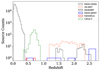 |
Fig. 1. Redshift distribution of the galaxies in all spectroscopic datasets. |
Number of galaxies per spectroscopic dataset, with conditions as defined in the text.
3. Low-redshift results
In this section we re-explore a diagram with blue emission lines, using a combination of EWs and flux ratios to understand the properties of the galaxies. We then separate the populations apparent in this diagram.
Emission line ratios measure the properties of the gas inside a galaxy (i.e. gas density, ionisation parameter). Instead, EWs measure the properties of the ionisation inside the galaxy (i.e. number of ionising photons, power of the ionising agent), assuming that the fraction of escaping ionising photons is negligible (Cid Fernandes et al. 2010; Stasińska et al. 2015).
Combining both of these observables should be a valuable tool to help us separate galaxy types. There are many examples of this approach, but one that is rarely used to separate galaxies comes in the form of comparing the EW of Hβ with the emission line flux ratio of [OIII]λ5007 and Hβ. We named it the OB-I (read as Oh-Bee-One) diagram, as it uses ionised states of oxygen and hydrogen (namely, hydrogen beta).
The FADO-SDSS sample (described in Sect. 2.1) provides us with a sample of a high volume of galaxies in the Local Universe and beyond (z ≲ 0.4), where the classification capabilities of the OB-I can be tested. The distribution of this data in the OB-I diagram can be seen in the left panel of Fig. 2, which shows that there seem to be two main clusters of data in the parameter space: a ‘cloud’ on the top that has more dispersed data, and a teardrop-shaped region which is more densely populated.
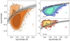 |
Fig. 2. OB-I diagram, with our empirical separation line. On all plots, the black curve and the grey shaded region represent our empirical separation line (see Eq. (2)). Left: FADO-SDSS sample (orange dots), as described in Sect. 2.1. The error bar represents the median error for all the points. Each contour represents 25% more of the sample, from the smallest to the largest. Right: NII-SF galaxies (top) and NII-AGN galaxies (bottom) that we used to define the empirical line. |
To separate these two regions, we can proceed through three main ways: using fully theoretical models (e.g. Kewley et al. 2001), fully empirical models (e.g. Veilleux & Osterbrock 1987), or a combination of the two, i.e. a semi-empirical model (e.g. Kauffmann et al. 2003). Since we are using the results from the data alone, we opted for a fully empirical approach. However, using only the two apparent clusters as a basis of galaxy classification is an unclear method, as the edges of a distribution are bound to be less dense and more scattered. Therefore, we used the classification from the NII diagram (or comparing [NII]λ6584/Hα with [OIII]λ5007/Hβ) as a basis to separate these two apparent galaxy populations. There are three types of galaxies, using the separation lines from Kewley et al. (2001) and Kauffmann et al. (2003): SF, Composite, and AGN, which from now on we call NII-SF, NII-Composite, and NII-AGN. We have 137 181 NII-SF galaxies, 16 990 NII-Composites, and 6890 NII-AGNs in the FADO-SDSS sample. We focus on NII-SF and NII-AGN to create our separation line.
In the right panel of Fig. 2 we can see that the NII-AGNs are mostly concentrated at the top left of the OB-I diagram, generally occupying a different space from the NII-SF galaxies, which are spread throughout the parameter space, preserving the teardrop shape that was mentioned above. In order to separate these two now evident populations, SF and AGN, we focused on fitting a general hyperbolic line with three parameters, given by the following equation:
![Mathematical equation: $$ \begin{aligned} \log \left(\frac{[\mathrm{OIII}]\lambda 5007}{\mathrm{H}\beta }\right) = \frac{a}{\log (\mathrm{EW}(\mathrm{H}\beta )) + b}+c. \end{aligned} $$](/articles/aa/full_html/2025/09/aa54528-25/aa54528-25-eq1.gif) (1)
(1)
We decided on this equation form because the frontier of the NII-SF population has a hyperbolic shape. To fit the three parameters on the equation, we enforced a simple criterion: the number of NII-SF and NII-AGNs that cross our empirical separation line has to be minimised; in other words, we want the smallest number of NII-SF galaxies crossing into the AGN region, and vice versa. Calculating the variables of the hyperbole by brute-force estimation, we found that the best equation that fits this criterion is the following:
![Mathematical equation: $$ \begin{aligned}&\log \left(\frac{[\mathrm{OIII}]\lambda 5007}{\mathrm{H}\beta }\right) = \frac{-3.00}{\log (\mathrm{EW}(\mathrm{H}\beta )) + (1.39\pm 0.07)} \nonumber \\&\qquad \qquad \qquad \qquad \qquad \qquad \qquad \qquad + (1.73\pm 0.13). \end{aligned} $$](/articles/aa/full_html/2025/09/aa54528-25/aa54528-25-eq2.gif) (2)
(2)
The uncertainties associated with our values come from the median uncertainties associated with all the galaxies in our sample. Overall, we find that 521 NII-SF galaxies (or 13% of the full NII-SF population) cross over into the AGN region, while 1068 NII-AGNs (or 18% of the full NII-AGN population) cross over into the SF region. In Fig. 3, we can see these results, and when we adopt our current empirical classification and apply them to the NII diagram (see Sect. 4.1 for more insights).
 |
Fig. 3. Match between NII and OB-I classes. This tells us how many galaxies in one classification belong to another; for example, the bottom left square shows that 19% of OB-I AGNs are classified as SF by the NII diagram. |
Something to note is that the EWs measured by FADO are about 25% higher than the EWs measured using the pseudo-continuum (Miranda et al. 2023). We checked to see if the position of our separation line was dependent on the methodology used to measure EWs. By adopting the Brinchmann et al. (2008) measurements provided in the MPA-JHU analysis for the same galaxies7, who used a different measurement method from the one used in FADO, we found very similar positions of both the NII-SF and NII-AGN populations (a maximum of 0.1 dex separation). This allows us to conclude that our separation line remains valid even for different ways of measuring EWs.
We are now in possession of a simple optical classification scheme that divides the FADO-SDSS sample in two: 153 983 objects are SF galaxies and 7104 are AGNs (considering the line only, and not the uncertainties). In order to further understand what drives the separation between these two galaxy populations, we can look at the emission line ratios and the EWs and try to understand the physical processes at play.
High values of the emission line flux ratio of [OIII]λ5007 and Hβ primarily reflects a high ionisation parameter (see e.g. Fig. 5 in Brinchmann 2023) or can be reproduced by shocks (Allen et al. 2008). In the case of the former, higher values of the ionisation parameter can typically occur either in low-metallicity starburst galaxies (e.g. blue compact dwarfs) or in AGNs. As for shocks, these usually require galaxies that are interacting or merging. Statistically, we do not expect our FADO-SDSS sample, which is a low-redshift sample, to be dominated by low-metallicity starburst galaxies nor by mergers and/or interactions between galaxies, so the upper part of the OB-I diagram should likely be populated by AGNs.
For the EW of Hβ, a combination of different physical mechanisms are at play, complicating the interpretation of the values observed. On the one hand, the EWs in SF galaxies scale linearly with the specific star formation rate of a galaxy (defined as the star formation divided by the stellar mass of the galaxy; see Fig. 3 of Casado et al. 2015), implying that high star formation rates give us higher equivalent widths. On the other hand, the EWs also depend on numerous other factors, such as gas-phase metallicity (Papaderos et al. 2023) and Lyman-continuum escape fraction (Papaderos et al. 2013), and we cannot discount the effects of the aperture of the SDSS fibres (Lagos et al. 2022). Because AGNs have a higher production rate of the Lyman-continuum than SF galaxies, one would expect them to have higher EWs, but the AGN continuum is both thermal and non-thermal, making it very bright, which in turn reduces the EW of an emission line.
Combining the information from the flux ratio and the EWs, it makes sense that AGNs – which are objects with high ionisation parameters, harder ionising fields, low star formation rates, and high continua values – are trapped in the upper left corner of the diagram where the [OIII]λ5007/Hβ flux ratio is high and EWs are low, while SF galaxies – which have a higher degree of star formation and usually lower continua than AGNs – are mostly in the lower parts of the diagram and can reach significantly higher EWs.
4. Discussion
In the previous section, we created a simple empirical line in the OB-I diagram that is separates galaxies into two types: SF-dominated galaxies and AGNs. In this section we discuss the ramifications of our classification. First, we take into account some caveats in the NII diagram classification; secondly, we compare the OB-I classification with another BPT diagram; and finally, we test our empirical line against theoretical models to find the physical origin for this separation.
4.1. Notes on the NII diagram
The NII diagram is one of the most commonly used classification schemes; it has been studied by several authors to distinctly separate galaxy types (e.g. Baldwin et al. 1981; Veilleux & Osterbrock 1987; Kewley et al. 2001, 2006; Kauffmann et al. 2003; Schawinski et al. 2007). However, it is known that the NII diagram has some difficulties in classifying galaxies with low stellar mass and, more importantly, sub-solar metallicity, due to the relative decrease in nitrogen emission in comparison with hydrogen emission (Groves et al. 2006), placing these objects in the SF region when they really are very likely to have an AGN (Kewley et al. 2013; Polimera et al. 2022; Harish et al. 2023).
In Fig. 4, looking at the OB-I AGNs in the NII diagram, we can see that there is a separate population of these objects present in the SF region of the NII diagram. In order to see if the some of the discrepancies are explained by the effects of sub-solar metallicity, we made use of the MPA-JHU measurements of metallicity of SDSS-DR7 (Brinchmann et al. 2004; Tremonti et al. 2004) as the FADO analysis does not provide nebular metallicities. This gives us metallicity measurements for 548 of the OB-I AGNs that reside in the NII-SF or NII-Composite regions, of which 90% have sub-solar metallicities. Due to this, we removed these galaxies from our analysis, though their true nature is likely to be AGN rather than SF.
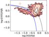 |
Fig. 4. OB-I AGNs in the NII diagram. The blue line represents the Kauffmann et al. (2003) separation line, while the black dashed line represents the Kewley et al. (2001) line. All the remaining elements are the same as in Fig. 2. |
For the NII-Composites, a direct comparison between the NII and OB-I diagrams is not straightforward. Firstly, this classification arises as a mixture between the semi-empirical fit of Kauffmann et al. (2003) and the theoretical fit of Kewley et al. (2001) in the NII diagram. Since they are not pure AGNs nor simply SF galaxies, they have been joined together as a type of galaxy whose emission comes from both sources. However, we can clearly see from Fig. 5 that these objects occupy a clear region in the parameter space, distinct from the AGN region and in the core of the SF region. Exploring these galaxies in more detail demands the use of and comparison with a theoretical photoionisation model, which is what we do in Sect. 4.3.
4.2. Comparison with SII diagram
Comparing the OB-I diagram with other classification schemes of the same nature allows us to have a better insight into how this diagram separates galaxy types. We have already used the NII diagram as a starting point to create our empirical line, but it is interesting to compare it with different BPT diagrams since they provide different information on the same set of galaxies. In this section we focus on the SII diagram (which compares the [SII]λλ6717, 6731/Hα and [OIII]λ5007/Hβ ratios).
We distinguish galaxy types in the SII diagram by using the Kewley et al. (2001) demarcation line, where we are presented with two classes: SII-SF and SII-AGN. In Fig. 6, we compare the classifications of the SII diagram with the OB-I diagram. Overall, we find a good agreement between these diagrams, where 98% of the SII-SF are correctly classified in the OB-I diagram, and 96% of the SII-AGN are correctly classified as well. On the other side, if we take the OB-I classification and apply it to the SII diagram, we also find a remarkable agreement with the SII classification, where 99% of the OB-I SF galaxies are in the SF region, and 59% of the OB-I AGNs are in the AGN region. All of this information is summarised in Fig. 7.
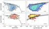 |
Fig. 6. Comparison between the SII diagram (left) and the OB-I diagram (right). In the OB-I diagram, the black line and the shaded region represent Eq. (2). In the SII diagram, the solid black line represents the separation by Kewley et al. (2001). Each contour represents 20% more of the sample, and the error bars represent the median error for each axis, for each classification. On the left is the OB-I classifications on the SII diagram; on the right is the SII classifications on the OB-I diagram. The top panels represent SF galaxies and bottom panels represent AGNs. |
When comparing the results of the NII and SII diagrams (Figs. 3 and 7), we expect the NII to have higher values of matched classification with the OB-I diagram rather than the SII diagram, as our empirical classification is based on the NII diagram classes. Although that is true for the OB-I classification, if we focus on the BPT diagram classes, we find that, surprisingly, the SII diagram has higher values of matched AGNs when compared with the NII diagram. This is likely due to two reasons: (1) the SII diagram is more sensitive to weaker AGNs (Polimera et al. 2022), and the OB-I diagram is likely tracing these objects as well, and (2) the Composite objects are seen in the NII diagram, but are not distinguishable in either the SII or OB-I diagrams.
4.3. Theoretical models
We apply the evolutionary theoretical models of HII regions in SF galaxies, computed by Stasińska et al. (2001), to the OB-I diagram in order to understand what the theory says about our empirical separation. These models all start at 104 years, and follow a timestep of 106 years and assume a Salpeter (1955) IMF. We chose to compare three scenarios: (1) an extended burst of star formation (10 Myr) with an initial burst of 106 M⊙, upper stellar limit of 120 M⊙ in the IMF, and gas density of nH = 1 cm−3; (2) an instantaneous period of star formation with the same conditions as the previous scenario; and (3) an instantaneous period of star formation, with an initial burst of 109 M⊙, upper stellar limit of 120 M⊙ in the IMF, and gas density of nH = 2 × 102 cm−3. For all these scenarios, we selected four metallicites: 0.05, 0.2, 0.4, 1 Z⊙. We chose these scenarios because they encompass the conditions of a wide variety of environments and star formation activity across the period of a galaxy’s lifetime, meaning we could probe the OB-I diagram for many kinds of galaxies, and not just one specific situation. We do not presume that these theoretical models represent all possible scenarios present in galaxies, but by looking at some extreme cases, we can still meaningfully infer the physics behind this diagram.
In Fig. 8, the results of these computational models can be seen overplotted on the OB-I diagram. Across all the scenarios, we can see that there is a downwards trend with time in the values of the axis of the OB-I diagram, signalled by the black arrow. In other words, when a galaxy gets older, the EW of Hβ and the [OIII]λ5007/Hβ emission line ratio decline sharply. This sharp decline varies from scenario to scenario, starting at 14 Myr in scenario 1 and at 5 Myr in scenarios 2 and 3, but the meaning is the same: this represents when the massive stars fade, leaving only the less massive and less ionising stars, which in turn reduces the strength of the Hβ emission line relative to the [OIII]λ5007 emission line (Byler et al. 2017).
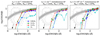 |
Fig. 8. Evolutionary models from Stasińska et al. (2001) overplotted on the OB-I diagram. From left to right, we have scenarios 1, 2, and 3 as described in the text (see Sect. 4.3). For all plots, the grey contours represent the FADO-SDSS sample; the black line is our separation line given by Eq. (2); the black arrow shows how the star-forming regions evolve with time; the blue markers and dashed line represent the model with 0.05 Z⊙; the green markers and solid line represent the model with 0.2 Z⊙; the red markers and dot-dashed line are the model with 0.4 Z⊙; and the cyan markers and solid line represent the model with Z⊙. The first marker of each metallicity is always on the top right of the OB-I diagram, and each subsequent marker represents a 2 Myr step for scenario 1 and a 1 Myr step for scenarios 2 and 3. The white triangle inside some markers represents the point where massive stars fade: 14 Myr for scenario 1 and 5 Myr for scenarios 2 and 3. |
Interestingly, we can see, in the early stages of the galaxies in all the scenarios, that the [OIII]λ5007/Hβ emission line ratio does not increase as the metallicity increases. There seems to be a distribution with a metallicity peak, meaning that for two different metallicities we obtain the same value for the [OIII]λ5007-to-Hβ ratio. This metallicity degeneracy has been noticed before in observations (Maiolino et al. 2008; Curti et al. 2017, 2020) and more recent work confirms this effect (see Fig. 4 of Nakajima et al. 2022), where the values for the ratio peak at around ≈0.2 Z⊙, which is the same prediction as in the models we are using.
Considering the 0.2 Z⊙ line as the edge limit case in all three scenarios, it is clear to see that for high values of the EW of Hβ (EW(Hβ)> 102 Å) there is a very good agreement with our separation line in the OB-I diagram, indicating that this is the limit that a SF galaxy can reach. Beyond this limit, any further contribution must come from another emission type rather than star formation, usually assumed to be an AGN. As we decrease the EW, especially in the scenarios where the SF episode is instantaneous, no model agrees with our separation line. In scenario 1, where there is an extended period of star formation, the 0.2 Z⊙ model agrees with our line until EW(Hβ)≈101.4 Å, but then we still have the aforementioned sharp decline.
This drop is present in all models and scenarios we considered. If we look at the core of the SF region, where most galaxies lie, we find that these objects lie typically above this drop. Since the models we are working with only consider star formation, then galaxies that have relatively high [OIII]λ5007/Hβ emission line ratios and low EWs of Hβ likely have a second process happening inside them that boosts the former, but not the latter. In Section 3, we already discussed that AGNs have high ionisation but retain low EWs; therefore, any object that is above the models and below our empirical line can belong to a mixed population, one that involves galaxies that are purely SF, have AGNs, and have activity from both (similar to the NII-Composites).
In order to separate this potential population, which we called mixed population due to their nature, from the AGNs and galaxies that only have star formation, we selected the points from each scenario that were as close to our empirical separation line as possible for all ages, no matter the metallicity; by this we mean that we selected the points that had the highest value of the [OIII]λ5007/Hβ emission line ratio at each age. Looking at Fig. 9, we can see that the mixed population is analogous to the NII-Composite galaxies, as they lie in the region above the points we chose. There are NII-SF galaxies in this region, but we argue that anything below our selection from the models should contain galaxies with star formation as the main (or even exclusive) source of emission, without AGN contamination, as they are fully encompassed by the Stasińska et al. (2001) models; we call these sources pure SF galaxies.
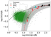 |
Fig. 9. Best fit model for the third population in the OB-I diagram. The grey contours represent the FADO-SDSS sample; the green points are the NII-Composite galaxies; the black line is our separation line given by Eq. (2); the black symbols represent the 0.2 Z⊙ model for all scenarios; the red symbols represent the 0.4 Z⊙ model for all scenarios; the cyan symbols represent the Z⊙ model for all scenarios. The red dot-dashed line represents the best fit for all the points in the diagram, given by Eq. (3). The grey shaded area represents the 1σ uncertainty associated with the fit. |
Afterwards, we chose four types of functions to fit onto the points: a linear fit; a second-degree polynomial; a third-degree polynomial; and a hyperbolic function of the same type as Eq. (1). To choose a function, we require two things: firstly, that the chosen fit has the lowest 1σ errors and, secondly, that it includes the smallest number of NII-Composites as possible below it. The second condition is important because the NII-Composites are an indicator of where the mixed population lies in the OB-I diagram. Therefore, if we want to create a separation line that includes solely galaxies whose main emission comes exclusively from SF, we need to exclude all components that might be mixed.
With these considerations in mind, the best fit we found was the following hyperbolic expression:
![Mathematical equation: $$ \begin{aligned}&\log \left(\frac{[\mathrm{OIII}]\lambda 5007}{\mathrm{H}\beta }\right) = \frac{-1.0\pm 0.2}{\log (\mathrm{EW}(\mathrm{H}\beta )) - (0.68\pm 0.09)} \nonumber \\&\qquad \qquad \qquad \qquad \qquad \qquad \qquad \qquad +(1.53\pm 0.12). \end{aligned} $$](/articles/aa/full_html/2025/09/aa54528-25/aa54528-25-eq3.gif) (3)
(3)
The results can be seen in Fig. 9.
At higher values of the EW of Hβ, this second separation line is extremely similar to the empirical line we calculated (Eq. (2)), providing further evidence that in this regime the separation between SF and AGN galaxies is clear.
In order to test whether the pure SF and the mixed populations are what we claim them to be, we can look once again at the NII and SII diagrams. From the top panels of Fig. 10 we can see that the pure SF population of the OB-I diagram fits quite nicely within the limits of the NII diagram SF region; only 3% of the OB-I pure SF galaxies cross over into the Composite and AGN territories. This implies that our modelled function of separation based on the Stasińska et al. (2001) models gives us a good estimate of the galaxies that are only forming stars and have no AGN influence, although we note that the low-metallicity regime is more complicated than both these diagrams make it seem. The bottom panels of Fig. 10 show that the same is true for the SII diagram, where again only 3% of the OB-I pure SF population crosses over into the AGN region. This reinforces the point that this population is made up of galaxies whose primary source of excitation comes from star formation, and essentially nothing else.
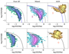 |
Fig. 10. NII (top) and SII (bottom) diagrams, compared with OB-I diagram classification. Left: OB-I pure SF galaxies. Each contour represents 20% more of the sample, and the error bar represents the median error for each axis. Middle: Same as left panel, but for OB-I mixed population. Right: Same as left panel, but for OB-I AGNs. All the remaining elements are the same as in Figs. 4 and 6. |
The mixed population is in line with what we expect it to be: a mix of galaxies with a combination of emissions from star formation and AGN, though the SF component still seems to dominate over the AGN component. Evidence for this comes from their position in the NII and SII diagrams, where most of them are placed in the SF region (88% in the NII-SF region and nearly 100% in the SII-SF region). Figure 11 shows these values with more detail, but overall, with the addition of Eq. (3), we can clearly see that we are able to improve the classification of galaxies that are purely SF, especially when compared to the NII diagram, with the detriment that the SII diagram seems to suffer from some loss in the classification. The AGN population does not undergo any alteration.
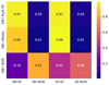 |
Fig. 11. Match between the OB-I classes and the NII and SII diagram regions. This tells us how many galaxies in the OB-I classification belongs to the NII or SII classes; for example, the top left square shows that 97% of OB-I pure SF are in the SF region of the NII diagram. |
However, the locations of these two populations show that the OB-I diagram (including Eqs. (2) and (3)) is still imperfect at distinguishing the mixed galaxy type. Nevertheless, we can claim that it is a good diagnostic tool of AGNs in the Local Universe and, through an analysis of theoretical models, can distinguish galaxies whose main source of emission comes exclusively from star formation. Any galaxy that has some sort of mixed regime is ambiguous as it becomes very difficult to tell what dominates their emission, the star formation or the AGN activity.
This discussion is limited to the Local Universe. In the next section we discuss how the OB-I diagram reacts to higher-redshift galaxies, how they evolve in the diagram, and what we can extract from it.
5. Higher-redshift landscape
It is known that line ratio diagrams are affected by a cosmic shift, where galaxies are placed in different positions in the parameter space depending on the redshift. The cause for this is still unknown, with explanations ranging from higher ionisation parameters of the gas in galaxies at higher redshifts (e.g. Brinchmann et al. 2008; Kewley et al. 2013), different contributions of the ionised gas and abundance ratios (e.g. Shapley et al. 2015; Cowie et al. 2016), differences in metallicity allowing stronger emission lines (e.g. Steidel et al. 2014, 2016), to the effects of shocks (Brinchmann 2023) or stellar rotation and binarity (Bian et al. 2020).
This implies that extrapolating the OB-I diagram from the Local Universe to a higher redshift is uncertain, as the cosmic shift can deeply impact this diagram, and therefore our empirical separation line. To measure this impact, we need to analyse the location of galaxies at higher redshifts in the OB-I diagram.
Our high-redshift sample was defined earlier in this work (see Sect. 2), where we have 1152 galaxies in the redshift range of 0.3 < z < 2.7, and includes data from LEGA-C, VANDELS, 3D-HST, MOSDEF, and FADO-JWST. This sample is by no means exhaustive, but it provides an idea of the limitations of the OB-I diagram at higher redshifts.
Each of these datasets has an AGN selection system, which is what we used for comparison with the OB-I diagram. As described in Sect. 2, the galaxies we selected from the VANDELS survey had no AGN flag, so they are very likely SF. Furthermore, the FADO-JWST galaxies were all selected to be SF galaxies.
For LEGA-C, 3D-HST, and MOSDEF, the process of selecting AGNs is more complicated. We describe the respective selection for each of these datasets in detail in Appendix A, but we present here a brief explanation. For LEGA-C, we made use of the flag_spec column, which detected 24 AGNs. For 3D-HST, we made use of IRAC photometry and the Donley et al. (2012) selection criteria, and found 20 galaxies to be AGNs. For MOSDEF, we made use of the NII diagram and the Kewley et al. (2013) selection criteria, and found three AGNs. All the remaining galaxies from these datasets are assumed to be SF.
In Fig. 12 we can see the whole higher-redshift sample on the OB-I diagram, separated into six different redshift bins, with AGNs classified from other schemes highlighted with a black circle. In Table 2 we list the summary information of these different classifications, including how many AGNs match the OB-I classification, and how many AGNs in total the OB-I actually identifies. We can see that the OB-I diagram can track down approximately 50% of AGNs found by different classification schemes without the need for significant adjustments in our empirical line.
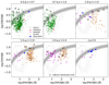 |
Fig. 12. OB-I diagram of the higher-redshift sample. The green diamonds represent the LEGA-C sample, the red triangles the VANDELS sample, the orange circles the 3D-HST sample, the magenta stars the MOSDEF sample, and the blue squares the FADO-JWST sample. The encircled symbols represent galaxies that are classified as AGNs by a separate classification scheme (see Appendix A). The grey contours represent the FADO-SDSS sample. The black dashed line is the separation line we defined in Eq. (2). The defined redshift bin is shown above each panel. |
AGNs found by each higher-redshift dataset considered in this work, by the OB-I diagram, and the match between them.
Notably, as we move from the lowest redshift to the highest redshift bins the number of identified AGNs is ever lower, in both the OB-I diagram and different galaxy classification schemes. This is likely due to the scarcity of sources observed and classified at redshifts above z > 2.4.
In Fig. 13, we compare the galaxies in our higher-redshift sample with the expected redshift evolution of EW(Hβ) from Khostovan et al. (2016). There are two caveats in this work that are worth discussing: first, they used galaxies that were both SF and AGNs and second, these classifications were based on EWs measured using photometric filters, which even in the narrow band could include effects from the [OIII]λ5007 emission line. The first point does not cause any issues for us since our sample is also a mixture of SF galaxies and AGNs. The second point could be a problem, but the authors used data from several datasets to constrain the fit, allowing it to be compared with other methods. Another point to add is that, as mentioned before, FADO measures EWs differently when compared to other methods, but even taking into account this effect, the difference is about 0.1 dex, not enough to change the location of these galaxies significantly.
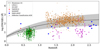 |
Fig. 13. Evolution of the EW(Hβ) with redshift. The black line and grey shaded area are the expected evolution from Khostovan et al. (2016). The white crosses represent the OB-I AGNs. All the remaining elements are the same as in Fig. 12. |
Overall, 53% of the galaxies are included in the expected redshift evolution of EW(Hβ), showing that more than one-half of our sample still follows the trend of increasing EW with redshift. It is of note that the AGNs from the OB-I or the aforementioned classification schemes (in white crosses and black circles, respectively) show only a slight trend with redshift and remain at low EW values. This is something we expected, as we explained at the end of Sect. 3.
The flux ratio of [OIII]λ5007/Hβ appears to increase as we increase the redshift as well, even in our limited sample. This is in line with recent galaxy samples obtained using JWST, such as the Assembly of Ultradeep Rest-optical Observations Revealing Astrophysics (AURORA) survey, where a subtle increase in the flux ratio is expected in the range 1.4 < z < 4.0 (Shapley et al. 2025), where most of our galaxies in the higher-redshift sample lie.
Another important facet to mention is that we are assuming that the classification from the datasets in our higher-redshift sample are correctly classifying their galaxies. All of the classification methods mentioned in Appendix A separate galaxies into two types (SF and AGN), but the truth is that many of these likely lie in the middle, similar to the NII-Composites in the Local Universe. Our current paradigm in the Cosmic Noon lacks the density of detected sources as in the Local Universe, so differentiating a third population at higher redshifts can only be done with, for example, spatially resolved and high-resolution data (e.g. Lam et al. 2025). With this in mind, we still argue that, despite all of these uncertainties, the OB-I diagram would add an element to dispel the differences between galaxies that have mixed SF and AGN influence, from the purely AGNs, since galaxies do not seem to evolve significantly with redshift in the range we are studying.
Keeping all these considerations in mind, we argue that the OB-I diagram, at least our empirical separation of galaxies, appears to be resistant to the cosmic shift that plagues most optical classification schemes. It has some success at classifying AGNs that other classification schemes identify, though there are still some that fall below our empirical separation line. Even with this setback (which we can clearly see in the 1 < z < 1.5 bin), the fact that the AGNs classified by other methods still lie in the uncertainty region of our empirical line is very encouraging. Furthermore, the overwhelming majority of the galaxies are correctly classified as SF-dominated galaxies across all redshifts, and there is no need for major adjustments unlike, for example, the SF-AGN line in Kewley et al. (2013). This can make the OB-I diagram and the empirical separation line we created a valuable tool, especially at redshifts between 1.7 < z < 2.7, where the Hα and [NII]λ6584 lines disappear out of the range of most optical spectrographs, leaving us with very few emission lines to work with. However, we need larger samples to further test these conclusions.
6. Conclusions and future work
Over the course of this work we explored the OB-I diagram, which compares the EW of Hβ and the emission line ratio of [OIII]λ5007/Hβ, in order to understand its properties and evolution. We selected 162 239 galaxies from the SDSS, LEGA-C, VANDELS, 3D-HST, MOSDEF, and JADES surveys in order to understand the properties and evolution of the OB-I diagram (see Table 1 and Fig. 1).
The FADO-SDSS sample was first plotted on the OB-I diagram as an analogue population for the Local Universe, and two clusters were apparent in the classification scheme: one dispersed in a cloud region and the other concentrated in an apparent teardrop-shaped region. To separate these two regions, we used the NII diagram (comparing [NII]λ6584/Hα with [OIII]λ5007/Hβ) to create an empirical line, given by Eq. (2) that essentially distinguishes between galaxies with a strong AGN contribution and galaxies with SF-dominated emission (see Fig. 2). We further compared this classification with the SII diagram, and found that 99% of the OB-I SF galaxies are below the Kewley et al. (2001) theoretical maximum starburst line and that 60% of the OB-I AGNs were above this same line (see Fig. 6). This tells us that there is a remarkably good agreement with the SII diagram classification, meaning that our empirical classification scheme is in line with the current paradigm of galaxy classification.
We further compared the OB-I diagram with the stellar evolution models of Stasińska et al. (2001), which can be seen in Fig. 8. From these models we reached two conclusions: (1) at higher values of EW of Hβ (above ≈102 Å) the models agree with our empirical classification line, meaning that the theory agrees with our separation between SF galaxies and AGNs, and (2) below this value the models show a sharp drop in the [OIII]λ5007/Hβ emission line ratio, implying the presence of a third population. This leads to an additional separation for the SF-dominated population in the OB-I diagram: one is made up of galaxies with only SF emission and the other is composed of galaxies with SF and AGN emission mixed together. We created a line, given by Eq. (3), to separate these two populations, although we note that there are many galaxies in the mixed population that are likely SF only, with no AGN contribution; however, we argue that galaxies below this line are mostly purely SF (see Fig. 10).
Finally, and most importantly, we compared the OB-I diagram with the higher-redshift sample (0.3 < z < 2.7), which includes the LEGA-C, VANDELS, MOSDEF, 3D-HST, and JADES surveys (Fig. 12). We found that our empirical classification scheme appears to be resistant to the cosmic shift that plagues most classification schemes in the optical (Brinchmann et al. 2008; Steidel et al. 2014, 2016; Shapley et al. 2015; Cowie et al. 2016; Brinchmann 2023; Bian et al. 2020). From flags and other classification schemes, we find that at higher redshifts the OB-I diagram correctly classifies one-half of the AGNs, with possibly no dependance on their redshift. With this in mind, we argue that the OB-I can be a valuable tool for classifying galaxies, with no need for modifications in separation lines according to redshift. In higher-redshift sources where emission lines such as Hα and [NII]λ6584 (which are required for other diagrams) are unavailable or hard to detect, the OB-I diagram acts as a first filter to understand the type of galaxies we are working with.
In the future, we plan on further exploring the redshift evolution of the OB-I diagram in more detail by using data from future surveys, such as the MOONS Redshift-Intensive Survey Experiment (MOONRISE, Cirasuolo & MOONS Consortium 2016; Cirasuolo et al. 2020; Maiolino et al. 2020), the Prime Focus Spectrograph (PFS, Takada et al. 2014), and the WHT Enhanced Area Velocity Explorer (WEAVE, Dalton 2016), as well as by generating theoretical models we can compare this data to.
Acknowledgments
This work was supported by Fundação para a Ciência e a Tecnologia (FCT) through the research grants PTDC/FIS-AST/29245/2017, UIDB/04434/2020 and UIDP/04434/2020. D.M.S. would like to acknowledge the meaningful discussions with Bruno Arsioli, who provided interesting insights to the paper. He would also like to acknowledge the patience and commitment of the team at the OAL and the IA, as well as the incredibly fruitful exchanges with C.L.. C.P. acknowledges support from DL 57/2016 (P2460) from the ‘Departamento de Física, Faculdade de Ciências da Universidade de Lisboa’. H.M. acknowledges support from the Fundação para a Ciência e a Tecnologia (FCT) through the PhD Fellowship 2022.12891.BD. R.C. acknowledges support from the Fundação para a Ciência e a Tecnologia (FCT) through the Fellowship PD/BD/150455/2019 (PhD:SPACE Doctoral Network PD/00040/2012) and POCH/FSE (EC). P.L. gratefully acknowledges support by the GEMINI ANID project No. 32240002. Funding for the SDSS and SDSS-II has been provided by the Alfred P. Sloan Foundation, the Participating Institutions, the National Science Foundation, the U.S. Department of Energy, the National Aeronautics and Space Administration, the Japanese Monbukagakusho, the Max Planck Society, and the Higher Education Funding Council for England. The SDSS Web Site is http://www.sdss.org/. The SDSS is managed by the Astrophysical Research Consortium for the Participating Institutions. The Participating Institutions are the American Museum of Natural History, Astrophysical Institute Potsdam, University of Basel, University of Cambridge, Case Western Reserve University, University of Chicago, Drexel University, Fermilab, the Institute for Advanced Study, the Japan Participation Group, Johns Hopkins University, the Joint Institute for Nuclear Astrophysics, the Kavli Institute for Particle Astrophysics and Cosmology, the Korean Scientist Group, the Chinese Academy of Sciences (LAMOST), Los Alamos National Laboratory, the Max-Planck-Institute for Astronomy (MPIA), the Max-Planck-Institute for Astrophysics (MPA), New Mexico State University, Ohio State University, University of Pittsburgh, University of Portsmouth, Princeton University, the United States Naval Observatory, and the University of Washington. This work would also like to acknowledge the support from Matplotlib (Hunter 2007). This work is based on observations taken by the 3D-HST Treasury Program (GO 12177 and 12328) with the NASA/ESA HST, which is operated by the Association of Universities for Research in Astronomy, Inc., under NASA contract NAS5-26555. The UKIDSS project is defined in Lawrence et al. ( 2007). Further details on the UDS can be found in Almaini et al. (2007). UKIDSS uses the UKIRT Wide Field Camera (WFCAM; Casali et al. 2007). The photometric system is described in Hewett et al. (2006), and the calibration is described in Hodgkin et al. (2009). The pipeline processing and science archive are described in Irwin et al. (2004) and Hambly et al. (2008). This study makes use of data from AEGIS, a multiwavelength sky survey conducted with the Chandra, GALEX, Hubble, Keck, CFHT, MMT, Subaru, Palomar, Spitzer, VLA, and other telescopes and supported in part by the NSF, NASA, and the STFC. This work is based, in part, on observations made with the Spitzer Space Telescope, which was operated by the Jet Propulsion Laboratory, California Institute of Technology under a contract with NASA.
References
- Abazajian, K. N., Adelman-McCarthy, J. K., Agüeros, M. A., et al. 2009, ApJS, 182, 543 [Google Scholar]
- Allen, M. G., Groves, B. A., Dopita, M. A., Sutherland, R. S., & Kewley, L. J. 2008, ApJS, 178, 20 [Google Scholar]
- Almaini, O., Foucaud, S., Lane, K., et al. 2007, ASP Conf. Ser., 379, 163 [NASA ADS] [Google Scholar]
- Alongi, M., Bertelli, G., Bressan, A., et al. 1993, A&AS, 97, 851 [NASA ADS] [Google Scholar]
- Backhaus, B. E., Trump, J. R., Cleri, N. J., et al. 2022, ApJ, 926, 161 [NASA ADS] [CrossRef] [Google Scholar]
- Baldwin, J. A., Phillips, M. M., & Terlevich, R. 1981, PASP, 93, 5 [Google Scholar]
- Bian, F., Kewley, L. J., Groves, B., & Dopita, M. A. 2020, MNRAS, 493, 580 [NASA ADS] [CrossRef] [Google Scholar]
- Brammer, G. B., van Dokkum, P. G., Franx, M., et al. 2012, ApJS, 200, 13 [Google Scholar]
- Bressan, A., Fagotto, F., Bertelli, G., & Chiosi, C. 1993, A&AS, 100, 647 [NASA ADS] [Google Scholar]
- Brinchmann, J. 2023, MNRAS, 525, 2087 [NASA ADS] [CrossRef] [Google Scholar]
- Brinchmann, J., Charlot, S., White, S. D. M., et al. 2004, MNRAS, 351, 1151 [Google Scholar]
- Brinchmann, J., Pettini, M., & Charlot, S. 2008, MNRAS, 385, 769 [NASA ADS] [CrossRef] [Google Scholar]
- Bruzual, G., & Charlot, S. 2003, MNRAS, 344, 1000 [NASA ADS] [CrossRef] [Google Scholar]
- Bunker, A. J., Cameron, A. J., Curtis-Lake, E., et al. 2024, A&A, 690, A288 [NASA ADS] [CrossRef] [EDP Sciences] [Google Scholar]
- Byler, N., Dalcanton, J. J., Conroy, C., & Johnson, B. D. 2017, ApJ, 840, 44 [Google Scholar]
- Calzetti, D., Armus, L., Bohlin, R. C., et al. 2000, ApJ, 533, 682 [NASA ADS] [CrossRef] [Google Scholar]
- Cardelli, J. A., Clayton, G. C., & Mathis, J. S. 1989, ApJ, 345, 245 [Google Scholar]
- Cardoso, L. S. M., Gomes, J. M., Papaderos, P., et al. 2022, A&A, 667, A11 [NASA ADS] [CrossRef] [EDP Sciences] [Google Scholar]
- Casado, J., Ascasibar, Y., Gavilán, M., et al. 2015, MNRAS, 451, 888 [NASA ADS] [CrossRef] [Google Scholar]
- Casali, M., Adamson, A., Alves de Oliveira, C., et al. 2007, A&A, 467, 777 [NASA ADS] [CrossRef] [EDP Sciences] [Google Scholar]
- Chabrier, G. 2003, ApJ, 586, L133 [NASA ADS] [CrossRef] [Google Scholar]
- Cid Fernandes, R., Stasińska, G., Schlickmann, M. S., et al. 2010, MNRAS, 403, 1036 [Google Scholar]
- Cid Fernandes, R., Stasińska, G., Mateus, A., & Vale Asari, N. 2011, MNRAS, 413, 1687 [Google Scholar]
- Cirasuolo, M., & MOONS Consortium 2016, ASP Conf. Ser., 507, 109 [NASA ADS] [Google Scholar]
- Cirasuolo, M., Fairley, A., Rees, P., et al. 2020, The Messenger, 180, 10 [NASA ADS] [Google Scholar]
- Cowie, L. L., Barger, A. J., & Songaila, A. 2016, ApJ, 817, 57 [NASA ADS] [CrossRef] [Google Scholar]
- Curti, M., Cresci, G., Mannucci, F., et al. 2017, MNRAS, 465, 1384 [Google Scholar]
- Curti, M., Mannucci, F., Cresci, G., & Maiolino, R. 2020, MNRAS, 491, 944 [Google Scholar]
- Dalton, G. 2016, ASP Conf. Ser., 507, 97 [Google Scholar]
- Davis, M., Guhathakurta, P., Konidaris, N. P., et al. 2007, ApJ, 660, L1 [NASA ADS] [CrossRef] [Google Scholar]
- Denicoló, G., Terlevich, R., & Terlevich, E. 2002, MNRAS, 330, 69 [CrossRef] [Google Scholar]
- DESI Collaboration (Adame, A. G., et al.) 2024, AJ, 168, 58 [NASA ADS] [CrossRef] [Google Scholar]
- Dickinson, M., Giavalisco, M., & GOODS Team 2003, in The Mass of Galaxies at Low and High Redshift, eds. R. Bender, & A. Renzini, 324 [Google Scholar]
- Donley, J. L., Koekemoer, A. M., Brusa, M., et al. 2012, ApJ, 748, 142 [Google Scholar]
- Eisenstein, D. J., Johnson, B. D., Robertson, B., et al. 2023a, ApJS, submitted [arXiv:2310.12340] [Google Scholar]
- Eisenstein, D. J., Willott, C., Alberts, S., et al. 2023b, ApJS, submitted [arXiv:2306.02465] [Google Scholar]
- Fagotto, F., Bressan, A., Bertelli, G., & Chiosi, C. 1994a, A&AS, 104, 365 [NASA ADS] [Google Scholar]
- Fagotto, F., Bressan, A., Bertelli, G., & Chiosi, C. 1994b, A&AS, 105, 29 [NASA ADS] [Google Scholar]
- Fazio, G. G., Hora, J. L., Allen, L. E., et al. 2004, ApJS, 154, 10 [Google Scholar]
- Feuillet, L. M., Meléndez, M., Kraemer, S., et al. 2024, ApJ, 962, 104 [NASA ADS] [CrossRef] [Google Scholar]
- Fukugita, M., Ichikawa, T., Gunn, J. E., et al. 1996, AJ, 111, 1748 [Google Scholar]
- Gardner, J. P., Mather, J. C., Clampin, M., et al. 2006, Space Sci. Rev., 123, 485 [Google Scholar]
- Garilli, B., McLure, R., Pentericci, L., et al. 2021, A&A, 647, A150 [NASA ADS] [CrossRef] [EDP Sciences] [Google Scholar]
- Girardi, L., Bressan, A., Chiosi, C., Bertelli, G., & Nasi, E. 1996, A&AS, 117, 113 [NASA ADS] [CrossRef] [EDP Sciences] [Google Scholar]
- Gomes, J. M., & Papaderos, P. 2017, A&A, 603, A63 [NASA ADS] [CrossRef] [EDP Sciences] [Google Scholar]
- Groves, B. A., Heckman, T. M., & Kauffmann, G. 2006, MNRAS, 371, 1559 [NASA ADS] [CrossRef] [Google Scholar]
- Gunn, J. E., Carr, M., Rockosi, C., et al. 1998, AJ, 116, 3040 [NASA ADS] [CrossRef] [Google Scholar]
- Hainline, K. N., Johnson, B. D., Robertson, B., et al. 2024, ApJ, 964, 71 [CrossRef] [Google Scholar]
- Hambly, N. C., Collins, R. S., Cross, N. J. G., et al. 2008, MNRAS, 384, 637 [NASA ADS] [CrossRef] [Google Scholar]
- Harish, S., Malhotra, S., Rhoads, J. E., et al. 2023, ApJ, 945, 157 [NASA ADS] [CrossRef] [Google Scholar]
- Hewett, P. C., Warren, S. J., Leggett, S. K., & Hodgkin, S. T. 2006, MNRAS, 367, 454 [Google Scholar]
- Hodgkin, S. T., Irwin, M. J., Hewett, P. C., & Warren, S. J. 2009, MNRAS, 394, 675 [CrossRef] [Google Scholar]
- Hunter, J. D. 2007, Comput. Sci. Eng., 9, 90 [NASA ADS] [CrossRef] [Google Scholar]
- Irwin, M. J., Lewis, J., Hodgkin, S., et al. 2004, SPIE Conf. Ser., 5493, 411 [Google Scholar]
- Juneau, S., Dickinson, M., Alexander, D. M., & Salim, S. 2011, ApJ, 736, 104 [Google Scholar]
- Kauffmann, G., Heckman, T. M., Tremonti, C., et al. 2003, MNRAS, 346, 1055 [Google Scholar]
- Kewley, L. J., & Dopita, M. A. 2002, ApJS, 142, 35 [Google Scholar]
- Kewley, L. J., Dopita, M. A., Sutherland, R. S., Heisler, C. A., & Trevena, J. 2001, ApJ, 556, 121 [Google Scholar]
- Kewley, L. J., Groves, B., Kauffmann, G., & Heckman, T. 2006, MNRAS, 372, 961 [Google Scholar]
- Kewley, L. J., Maier, C., Yabe, K., et al. 2013, ApJ, 774, L10 [Google Scholar]
- Khostovan, A. A., Sobral, D., Mobasher, B., et al. 2016, MNRAS, 463, 2363 [Google Scholar]
- Kriek, M., Shapley, A. E., Reddy, N. A., et al. 2015, ApJS, 218, 15 [NASA ADS] [CrossRef] [Google Scholar]
- Lagos, P., Loubser, S. I., Scott, T. C., et al. 2022, MNRAS, 516, 5487 [NASA ADS] [CrossRef] [Google Scholar]
- Lam, N., Shapley, A. E., Sanders, R. L., et al. 2025, ApJ, submitted [arXiv:2506.22547] [Google Scholar]
- Lawrence, A., Warren, S.~J., Almaini, O., et al. 2007, MNRAS, 379, 1599 [NASA ADS] [CrossRef] [Google Scholar]
- LeFevre, O., Saisse, M., Mancini, D., et al. 2003, Int. Soc. Opt. Photon., 4841, 1670 [Google Scholar]
- Madau, P., & Dickinson, M. 2014, ARA&A, 52, 415 [Google Scholar]
- Maiolino, R., Nagao, T., Grazian, A., et al. 2008, A&A, 488, 463 [NASA ADS] [CrossRef] [EDP Sciences] [Google Scholar]
- Maiolino, R., Cirasuolo, M., Afonso, J., et al. 2020, The Messenger, 180, 24 [NASA ADS] [Google Scholar]
- Mazzolari, G., Übler, H., Maiolino, R., et al. 2024, A&A, 691, A345 [NASA ADS] [CrossRef] [EDP Sciences] [Google Scholar]
- McLean, I. S., Steidel, C. C., Epps, H. W., et al. 2012, SPIE Conf. Ser., 8446, 84460J [NASA ADS] [Google Scholar]
- McLure, R. J., Pentericci, L., Cimatti, A., et al. 2018, MNRAS, 479, 25 [NASA ADS] [Google Scholar]
- Miranda, H., Pappalardo, C., Papaderos, P., et al. 2023, A&A, 669, A16 [NASA ADS] [CrossRef] [EDP Sciences] [Google Scholar]
- Momcheva, I. G., Brammer, G. B., van Dokkum, P. G., et al. 2016, ApJS, 225, 27 [Google Scholar]
- Nakajima, K., Ouchi, M., Xu, Y., et al. 2022, ApJS, 262, 3 [CrossRef] [Google Scholar]
- Osterbrock, D., & Ferland, G. 2006, Astrophysics Of Gas Nebulae and Active Galactic Nuclei (Sausalito: University Science Books) [Google Scholar]
- Paalvast, M., Verhamme, A., Straka, L. A., et al. 2018, A&A, 618, A40 [NASA ADS] [CrossRef] [EDP Sciences] [Google Scholar]
- Papaderos, P., Gomes, J. M., Vílchez, J. M., et al. 2013, A&A, 555, L1 [NASA ADS] [CrossRef] [EDP Sciences] [Google Scholar]
- Papaderos, P., Östlin, G., & Breda, I. 2023, A&A, 673, A30 [NASA ADS] [CrossRef] [EDP Sciences] [Google Scholar]
- Pentericci, L., McLure, R. J., Garilli, B., et al. 2018, A&A, 616, A174 [NASA ADS] [CrossRef] [EDP Sciences] [Google Scholar]
- Perrotta, S., George, E. R., Coil, A. L., et al. 2021, ApJ, 923, 275 [Google Scholar]
- Polimera, M. S., Kannappan, S. J., Richardson, C. T., et al. 2022, ApJ, 931, 44 [NASA ADS] [CrossRef] [Google Scholar]
- Reddy, N. A., Kriek, M., Shapley, A. E., et al. 2015, ApJ, 806, 259 [NASA ADS] [CrossRef] [Google Scholar]
- Rieke, M. J., Robertson, B., Tacchella, S., et al. 2023, ApJS, 269, 16 [NASA ADS] [CrossRef] [Google Scholar]
- Rola, C. S., Terlevich, E., & Terlevich, R. J. 1997, MNRAS, 289, 419 [NASA ADS] [Google Scholar]
- Salpeter, E. E. 1955, ApJ, 121, 161 [Google Scholar]
- Schawinski, K., Thomas, D., Sarzi, M., et al. 2007, MNRAS, 382, 1415 [Google Scholar]
- Schlafly, E. F., & Finkbeiner, D. P. 2011, ApJ, 737, 103 [Google Scholar]
- Schlegel, D. J., Finkbeiner, D. P., & Davis, M. 1998, ApJ, 500, 525 [Google Scholar]
- Scoville, N., Aussel, H., Brusa, M., et al. 2007, ApJS, 172, 1 [Google Scholar]
- Searle, L. 1972, in External Galaxies and Quasi-Stellar Objects, eds. D. S. Evans, D. Wills, & B. J. Wills, 44, 66 [Google Scholar]
- Shapley, A. E., Reddy, N. A., Kriek, M., et al. 2015, ApJ, 801, 88 [NASA ADS] [CrossRef] [Google Scholar]
- Shapley, A. E., Sanders, R. L., Topping, M. W., et al. 2025, ApJ, 980, 242 [Google Scholar]
- Skelton, R. E., Whitaker, K. E., Momcheva, I. G., et al. 2014, ApJS, 214, 24 [Google Scholar]
- Solimano, M., González-López, J., Aravena, M., et al. 2025, A&A, 693, A70 [NASA ADS] [CrossRef] [EDP Sciences] [Google Scholar]
- Stasińska, G., Schaerer, D., & Leitherer, C. 2001, A&A, 370, 1 [NASA ADS] [CrossRef] [EDP Sciences] [Google Scholar]
- Stasińska, G., Izotov, Y., Morisset, C., & Guseva, N. 2015, A&A, 576, A83 [NASA ADS] [CrossRef] [EDP Sciences] [Google Scholar]
- Steidel, C. C., Rudie, G. C., Strom, A. L., et al. 2014, ApJ, 795, 165 [Google Scholar]
- Steidel, C. C., Strom, A. L., Pettini, M., et al. 2016, ApJ, 826, 159 [NASA ADS] [CrossRef] [Google Scholar]
- Straatman, C. M. S., van der Wel, A., Bezanson, R., et al. 2018, ApJS, 239, 27 [NASA ADS] [CrossRef] [Google Scholar]
- Szokoly, G. P., Bergeron, J., Hasinger, G., et al. 2004, ApJS, 155, 271 [NASA ADS] [CrossRef] [Google Scholar]
- Takada, M., Ellis, R. S., Chiba, M., et al. 2014, PASJ, 66, R1 [Google Scholar]
- Talia, M., Schreiber, C., Garilli, B., et al. 2023, A&A, 678, A25 [NASA ADS] [CrossRef] [EDP Sciences] [Google Scholar]
- Teimoorinia, H., & Keown, J. 2018, MNRAS, 478, 3177 [Google Scholar]
- Teimoorinia, H., Shishehchi, S., Archinuk, F., et al. 2024, ApJ, 973, 95 [Google Scholar]
- Tremonti, C. A., Heckman, T. M., Kauffmann, G., et al. 2004, ApJ, 613, 898 [Google Scholar]
- van der Wel, A., Noeske, K., Bezanson, R., et al. 2016, ApJS, 223, 29 [Google Scholar]
- van der Wel, A., Bezanson, R., D’Eugenio, F., et al. 2021, ApJS, 256, 44 [NASA ADS] [CrossRef] [Google Scholar]
- Veilleux, S., & Osterbrock, D. E. 1987, ApJS, 63, 295 [Google Scholar]
- Werner, M. W., Roellig, T. L., Low, F. J., et al. 2004, ApJS, 154, 1 [NASA ADS] [CrossRef] [Google Scholar]
- York, D. G., Adelman, J., Anderson, J. E., et al. 2000, AJ, 120, 1579 [Google Scholar]
Appendix A: Higher-redshift AGN classification
In this Appendix we provide further information into how AGNs were estimated from the different datasets for our higher-redshift sample, described in Sects. 2 and 5. All the information on how many galaxies are classified as SF and AGN according to each dataset is summed in Table A.1.
SF galaxies and AGNs found by each higher-redshift dataset considered in this work.
A.1. LEGA-C
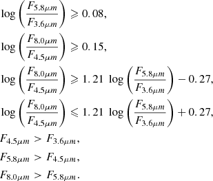
In the LEGA-C sample the flag_spec column lets us know that there is an AGN present in the sample if this flag is equal to 1. These objects were flagged as AGNs due to clear evidence that the continuum was affected by this component and this, in turn, affected the measurement of indices, which was confirmed by visual inspection. With this scheme, we mark 24 galaxies as AGNs, and the remaining 699 objects are likely to be SF. This sample can be seen on the OB-I diagram in Fig. A.1.
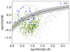 |
Fig. A.1. OB-I diagram with the LEGA-C sample. The blue stars represent AGNs according to the flag_spec criterium. The green diamonds represent SF galaxies. The grey contours represent the FADO-SDSS sample, and the black line and grey shaded area represent our empirical separation given by Eq. (2). |
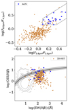 |
Fig. A.2. 3D-HST sample in an IRAC colour-colour plot (top) and the OB-I diagram (bottom). In the top panel, the black lines represent the area according to Eq. (A.1) that was used to identify AGNs (blue stars). All the remaining galaxies should be SF and are represented by orange dots. In the bottom panel stars and dots are the same as in the IRAC colour-colour plot. The grey contours represent the FADO-SDSS sample and the black line and grey shaded area represent our empirical separation given by Eq. (2). |
A.2. 3D-HST
Regarding 3D-HST data, we can use the available IRAC photometry to select AGNs. Using the classification scheme by Donley et al. (2012), a galaxy is defined as an AGN if it obeys the following conditions:
 (A.1)
(A.1)
Here F3.6μm, F4.5μm, F5.8μm, and F8.0μm represent flux densities at 3.6, 4.5, 5.8, and 8.0 microns, respectively. We decided on this classification scheme because these criteria have been mostly developed using non-local, obscured galaxies, allowing us to avoid any cosmic shift in the IRAC colour-colour plot. With these criteria, 20 galaxies are classified as AGNs, while the remaining 326 are expected to be SF. The colour-colour plot and the location of all galaxies in the OB-I diagram can be seen in top and bottom panels of Fig. A.2, respectively.
A.3. MOSDEF
In the MOSDEF data, we have all the necessary emission line fluxes to plot the NII diagram and compare it with the OB-I diagram. However, since we are working with redshifts above 1, we cannot use the classification schemes of Kewley et al. (2001) and Kauffmann et al. (2003), as they were optimised for the lower redshifts. In order to take into account the cosmic shift, we base ourselves on the theoretical work of Kewley et al. (2013) to separate galaxies between SF and AGN, as a function of redshift:
![Mathematical equation: $$ \begin{aligned}&\log \left(\frac{[\mathrm{OIII}]\lambda 5007}{\mathrm{H}\beta }\right) = \frac{0.61}{\log ([\mathrm{NII}]\lambda 6584/\mathrm{H}\alpha ) - 0.02 - 0.1833z} \nonumber \\&\qquad \qquad \qquad \qquad \qquad \qquad \qquad \qquad + 1.2 + 0.03z. \end{aligned} $$](/articles/aa/full_html/2025/09/aa54528-25/aa54528-25-eq5.gif) (A.2)
(A.2)
We took each galaxy present in the MOSDEF sample and applied this equation, to figure out if they are SF or AGN. With this classification scheme, we find that three galaxies are classified as AGN, while the remaining 67 are expected to be SF. The positions of these galaxies in the NII and OB-I diagrams can be seen in Fig. A.3.
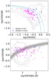 |
Fig. A.3. MOSDEF sample in the NII and OB-I diagrams. Top: NII diagram. The solid and dashed cyan lines represents the lowest and highest redshifts values from Eq. (A.2), respectively, for the galaxies in the MOSDEF sample. The magenta dots represent SF galaxies and the blue stars AGNs according to the aforementioned classification. The grey contours represent the FADO-SDSS sample. Bottom: OB-I diagram. The magenta dots and blue stars are the same as in the NII diagram. The grey contours represents the FADO-SDSS sample and the black line and grey shaded area represent our empirical separation given by Eq. (2). |
All Tables
Number of galaxies per spectroscopic dataset, with conditions as defined in the text.
AGNs found by each higher-redshift dataset considered in this work, by the OB-I diagram, and the match between them.
SF galaxies and AGNs found by each higher-redshift dataset considered in this work.
All Figures
|
Fig. 1. Redshift distribution of the galaxies in all spectroscopic datasets. |
| In the text | |
|
Fig. 2. OB-I diagram, with our empirical separation line. On all plots, the black curve and the grey shaded region represent our empirical separation line (see Eq. (2)). Left: FADO-SDSS sample (orange dots), as described in Sect. 2.1. The error bar represents the median error for all the points. Each contour represents 25% more of the sample, from the smallest to the largest. Right: NII-SF galaxies (top) and NII-AGN galaxies (bottom) that we used to define the empirical line. |
| In the text | |
|
Fig. 3. Match between NII and OB-I classes. This tells us how many galaxies in one classification belong to another; for example, the bottom left square shows that 19% of OB-I AGNs are classified as SF by the NII diagram. |
| In the text | |
|
Fig. 4. OB-I AGNs in the NII diagram. The blue line represents the Kauffmann et al. (2003) separation line, while the black dashed line represents the Kewley et al. (2001) line. All the remaining elements are the same as in Fig. 2. |
| In the text | |
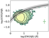 |
Fig. 5. NII-Composites in the OB-I diagram. All the remaining elements are the same as in Fig. 2. |
| In the text | |
|
Fig. 6. Comparison between the SII diagram (left) and the OB-I diagram (right). In the OB-I diagram, the black line and the shaded region represent Eq. (2). In the SII diagram, the solid black line represents the separation by Kewley et al. (2001). Each contour represents 20% more of the sample, and the error bars represent the median error for each axis, for each classification. On the left is the OB-I classifications on the SII diagram; on the right is the SII classifications on the OB-I diagram. The top panels represent SF galaxies and bottom panels represent AGNs. |
| In the text | |
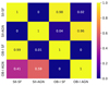 |
Fig. 7. Match between SII and OB-I classes. All are the same as in Fig. 3. |
| In the text | |
|
Fig. 8. Evolutionary models from Stasińska et al. (2001) overplotted on the OB-I diagram. From left to right, we have scenarios 1, 2, and 3 as described in the text (see Sect. 4.3). For all plots, the grey contours represent the FADO-SDSS sample; the black line is our separation line given by Eq. (2); the black arrow shows how the star-forming regions evolve with time; the blue markers and dashed line represent the model with 0.05 Z⊙; the green markers and solid line represent the model with 0.2 Z⊙; the red markers and dot-dashed line are the model with 0.4 Z⊙; and the cyan markers and solid line represent the model with Z⊙. The first marker of each metallicity is always on the top right of the OB-I diagram, and each subsequent marker represents a 2 Myr step for scenario 1 and a 1 Myr step for scenarios 2 and 3. The white triangle inside some markers represents the point where massive stars fade: 14 Myr for scenario 1 and 5 Myr for scenarios 2 and 3. |
| In the text | |
|
Fig. 9. Best fit model for the third population in the OB-I diagram. The grey contours represent the FADO-SDSS sample; the green points are the NII-Composite galaxies; the black line is our separation line given by Eq. (2); the black symbols represent the 0.2 Z⊙ model for all scenarios; the red symbols represent the 0.4 Z⊙ model for all scenarios; the cyan symbols represent the Z⊙ model for all scenarios. The red dot-dashed line represents the best fit for all the points in the diagram, given by Eq. (3). The grey shaded area represents the 1σ uncertainty associated with the fit. |
| In the text | |
|
Fig. 10. NII (top) and SII (bottom) diagrams, compared with OB-I diagram classification. Left: OB-I pure SF galaxies. Each contour represents 20% more of the sample, and the error bar represents the median error for each axis. Middle: Same as left panel, but for OB-I mixed population. Right: Same as left panel, but for OB-I AGNs. All the remaining elements are the same as in Figs. 4 and 6. |
| In the text | |
|
Fig. 11. Match between the OB-I classes and the NII and SII diagram regions. This tells us how many galaxies in the OB-I classification belongs to the NII or SII classes; for example, the top left square shows that 97% of OB-I pure SF are in the SF region of the NII diagram. |
| In the text | |
|
Fig. 12. OB-I diagram of the higher-redshift sample. The green diamonds represent the LEGA-C sample, the red triangles the VANDELS sample, the orange circles the 3D-HST sample, the magenta stars the MOSDEF sample, and the blue squares the FADO-JWST sample. The encircled symbols represent galaxies that are classified as AGNs by a separate classification scheme (see Appendix A). The grey contours represent the FADO-SDSS sample. The black dashed line is the separation line we defined in Eq. (2). The defined redshift bin is shown above each panel. |
| In the text | |
|
Fig. 13. Evolution of the EW(Hβ) with redshift. The black line and grey shaded area are the expected evolution from Khostovan et al. (2016). The white crosses represent the OB-I AGNs. All the remaining elements are the same as in Fig. 12. |
| In the text | |
|
Fig. A.1. OB-I diagram with the LEGA-C sample. The blue stars represent AGNs according to the flag_spec criterium. The green diamonds represent SF galaxies. The grey contours represent the FADO-SDSS sample, and the black line and grey shaded area represent our empirical separation given by Eq. (2). |
| In the text | |
|
Fig. A.2. 3D-HST sample in an IRAC colour-colour plot (top) and the OB-I diagram (bottom). In the top panel, the black lines represent the area according to Eq. (A.1) that was used to identify AGNs (blue stars). All the remaining galaxies should be SF and are represented by orange dots. In the bottom panel stars and dots are the same as in the IRAC colour-colour plot. The grey contours represent the FADO-SDSS sample and the black line and grey shaded area represent our empirical separation given by Eq. (2). |
| In the text | |
|
Fig. A.3. MOSDEF sample in the NII and OB-I diagrams. Top: NII diagram. The solid and dashed cyan lines represents the lowest and highest redshifts values from Eq. (A.2), respectively, for the galaxies in the MOSDEF sample. The magenta dots represent SF galaxies and the blue stars AGNs according to the aforementioned classification. The grey contours represent the FADO-SDSS sample. Bottom: OB-I diagram. The magenta dots and blue stars are the same as in the NII diagram. The grey contours represents the FADO-SDSS sample and the black line and grey shaded area represent our empirical separation given by Eq. (2). |
| In the text | |
Current usage metrics show cumulative count of Article Views (full-text article views including HTML views, PDF and ePub downloads, according to the available data) and Abstracts Views on Vision4Press platform.
Data correspond to usage on the plateform after 2015. The current usage metrics is available 48-96 hours after online publication and is updated daily on week days.
Initial download of the metrics may take a while.