| Issue |
A&A
Volume 701, September 2025
|
|
|---|---|---|
| Article Number | A102 | |
| Number of page(s) | 9 | |
| Section | Stellar structure and evolution | |
| DOI | https://doi.org/10.1051/0004-6361/202554636 | |
| Published online | 04 September 2025 | |
A detailed study on the pulse profile of PSR B0950+08
School of Physical Science and Technology, Southwest University, Chongqing, 400715
China
⋆ Corresponding author: This email address is being protected from spambots. You need JavaScript enabled to view it.
Received:
19
March
2025
Accepted:
6
July
2025
Abstract
The pulsar PSR B0950+08 is one of the brightest pulsars with extremely high flux intensity. To understand the pulse profile properties, we conducted a study using one hour of data from FAST observations, focusing on the shape of the average pulse profiles, polarization characteristics, and microstructure. We find that both the width of the average pulse profile and the fraction of linear polarization change with varying relative flux intensity. Moreover, we report, for the first time, a strong linear relationship between the profile width and the fraction of linear polarization for this pulsar. For average pulse profiles with different flux intensities, we observe jumps in the polarization position angle and changes in the profile shape. Distinct depolarization occurs at the polarization position angle jump, which is related to the pulsar’s flux intensity. By performing an autocorrelation analysis on the single pulses, we obtained the characteristic width and period of the microstructure.
Key words: polarization / pulsars: general / pulsars: individual: PSR B0950+08
© The Authors 2025
 Open Access article, published by EDP Sciences, under the terms of the Creative Commons Attribution License (https://creativecommons.org/licenses/by/4.0), which permits unrestricted use, distribution, and reproduction in any medium, provided the original work is properly cited.
This article is published in open access under the Subscribe to Open model. This email address is being protected from spambots. You need JavaScript enabled to view it. to support open access publication.
1. Introduction
Pulsars are rapidly rotating neutron stars that emit radio signals at stable periods, playing a significant role in interstellar navigation, gravitational wave detection, and other fields (Cordes et al. 2004). The average pulse profile, formed by folding a large number of single pulses, is relatively stable, whereas single pulses often reflect the most accurate representation of the pulsar radiation region (Gould & Lyne 1998). The polarization characteristics of single pulses help us to understand the geometric structure of the pulsar’s emission region. For the polarization position angle (PA) curve, many pulsars, though not all, exhibit a well-defined “S” shape, which can be explained by the rotating vector model (Radhakrishnan & Cooke 1969). Due to the presence of orthogonal polarization modes in the radiation, some pulsars display abrupt jumps in PA of around 90°. Orthogonal polarization modes are widely observed in both the average pulse profile and single pulses (Manchester et al. 1975). In addition, orthogonal polarization modes are a wide-band phenomenon. The radiation from one polarization mode instantaneously superimposes on that from the orthogonal mode, resulting in the depolarization observed in the polarization wave (Stinebring et al. 1984). Single pulses of some pulsars exhibit rapid variations on timescales of approximately 200 microseconds at 430 MHz (Craft et al. 1968). Observations of giant pulses from the Crab pulsar show that the timescale of pulse components can be as short as a few nanoseconds (Hankins 1996). Such short-timescale emission units are collectively referred to as microstructure.
The pulsar PSR B0950+08 is a relatively nearby, bright pulsar, located at a distance of approximately 0.26 kpc (Yao et al. 2017). Its rotation period is 253.07 ms (Hobbs et al. 2004), and the dispersion measure is 2.97 pc ⋅ cm−3 (Stovall et al. 2015). The average pulse profile of this pulsar consists of an interpulse and a main pulse connected by bridge radiation (Hankins & Cordes 1981), and it exhibits a strong dependence on frequency (Hankins et al. 1991; Kuzmin et al. 1998). Observations from the Five-hundred-meter Aperture Spherical radio Telescope (FAST) have confirmed that the pulsar radiation is present throughout the whole phase (Wang et al. 2022). Ul’yanov & Zakharenko (2012) calculated the cumulative and differential energy distributions of subpulse radio emission for this pulsar at a wavelength of ten meters. They compared the cumulative distribution with the characteristic distribution of giant pulses from giant-pulse pulsars, indicating that the amplification mechanisms producing giant pulses and abnormally strong pulses in the pulsar magnetosphere may be similar. The pulsar PSR B0950+08 exhibits short and bright pulses at low frequencies that resemble normal pulses rather than giant pulses (Bilous et al. 2022). Singh et al. (2024) find that the single pulses of this pulsar exhibit many complex PA jumps, which can be explained by the superposition of two coherent or incoherent orthogonal polarization waves. Microstructure is a ubiquitous feature of pulsar emission, with its short timescale reflecting the structure of the emission region (Lange et al. 1998). A study of abnormally strong pulses from PSR B0950+08 at a wavelength of ten meters reveals short microstructure with a timescale of 1 ms (Ulyanov et al. 2016). A large amount of quasiperiodic microstructure is observed in the single pulses of PSR B0950+08. At the 430 MHz observation frequency, the microstructure period ranges from 0.15 ms to 1.1 ms, with the most frequent periods being approximately 0.4 ms and 0.6 ms (Hankins & Boriakoff 1978).
As the world’s largest single-aperture radio telescope, FAST plays a crucial role in the study of pulsar radiation mechanisms and the detection of weak emissions because of its high sensitivity. In this paper, we primarily investigate the characteristics of PSR B0950+08 in terms of its average profile, orthogonal polarization modes, and microstructure. Section 2 describes the FAST observations and data processing. Section 3 presents the results of our research. Section 4 discusses the results, and Section 5 provides the conclusions.
2. Observation and data processing
The FAST facility is located in Guizhou Province, China, and has an effective aperture of 300 meters during normal operation, making it the world’s most sensitive single-aperture radio telescope (Jiang et al. 2019). We used data recorded on November 26, 2019 with a duration of one hour1. We conducted observations using the central beam of a 19-beam receiver, covering a frequency range from 1050 MHz to 1450 MHz, with a center frequency of 1250 MHz and a total of 4096 frequency channels. The data were stored in the PSRFITS file format in tracking mode, recording 14 231 single pulses, each with 5120 sampling points and a time resolution of 49.152 μs. We calibrated the data by injecting a stable noise signal with a period of 0.201326592 s using a single diode (Xie et al. 2022). We removed the effects of dispersion measure and Faraday rotation measure using the PAM command in the PSRCHIVE software package 2012ART....9..237V. We then used the PAZI command to remove the upper and lower 10% of the frequency bandwidth and interference of the narrowband radio frequency (Hotan et al. 2004). Finally, we performed polarization calibration using the PAC command to obtain the Stokes parameters. Since this paper focuses primarily on the characteristics of pulse profile shapes, we did not carry out absolute flux intensity calibration.
From the PSRFITS file, we obtained the four Stokes parameters: I, Q, U, and V. We used the off-pulse region as the noise level for baseline subtraction. The linear polarization is given by  . To eliminate the bias, the true value of linear polarization is given by the following:
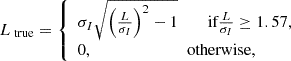 (1)
(1)
where σI is the standard deviation of the Stokes parameter I in the off-pulse region (Everett & Weisberg 2001). The PA can be calculated using  . Additionally, the uncertainty in PA is
  , where σU and σQ are the standard deviations of the Stokes parameters U and Q in the off-pulse region, respectively.
3. Result
3.1. The average pulse with different flux intensity
Figure 1 shows the total average pulse profile of PSR B0950+08, which is derived from the folding of 14 231 single pulses. The average pulse profile shows that this pulsar exhibits both an interpulse and a main pulse, each composed of multiple subcomponents. The inter pulse and the main pulse are connected by bridge radiation. The fraction of linear polarization (FL) in the main pulse is notably lower than that in the interpulse. In addition, the interpulse exhibits a weak left-handed circular polarization signal, whereas the main pulse shows a strong right-handed circular polarization signal. The total PA curve is very smooth, except for a bulge formed between 295° and 320°. We calculated the relative energy (Ere) for each single pulse, defined as Ere = E/⟨E⟩, where E and ⟨E⟩ represent the flux intensity of the single pulse and the total average pulse profile, respectively. The statistical distribution of Ere is shown in Fig. 2. We divided the single pulses into ten groups based on ascending values of Ere, then folded each group of single pulses to obtain their average pulse profile.
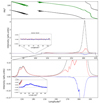 |
Fig. 1. Total average pulse profile of PSR B0950+08. The top panel shows the PA curve of the total average pulse profile with σψ < 5°, along with the curve of PA ± 180°. To facilitate analysis of PA properties, the green curve representing the continuous variation of PA is plotted. The middle panel displays the average pulse profiles of total intensity I (solid black line), linear polarization L (solid red line) and circular polarization V (solid blue line), respectively. The zoom-in box shows the noise level region. The bottom panel presents a zoomed-in view of the region as outlined by the dashed box in the middle panel. The zoomed-in view of the circular polarization of the interpulse is shown within the rectangular box in the bottom panel. |
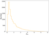 |
Fig. 2. Statistical distribution of Ere for 14 231 single pulses. |
Figure 3 presents the unnormalized average pulse profiles divided into ten groups based on Ere. For convenience, these average pulse profiles are named Profile 1 through Profile 10 in ascending order of Ere. The top panels show that the total intensity of the main pulse varies significantly, whereas the intensity of the interpulse shows smaller variations. This suggests that the total intensity changes are primarily caused by the main pulse. In addition, the shape and intensity of the interpulse in Profile 10 exhibit comparatively large variations, whereas the others remain relatively stable. In the middle panels, the linear polarization profile of the main pulse exhibits significant changes in both intensity and shape. In particular, the leading part of the main pulse in Profile 10 shows a distinct depolarization. Similarly, for the interpulse, the linear polarization profile of Profile 10 shows significant changes, whereas the others remain relatively stable. The bottom panels present the circular polarization profiles, where the circular polarization sign of the main pulse remains negative from Profile 1 to Profile 9, with only Profile 10 exhibiting a sign reversal in its leading part. Similarly, for the interpulse, only Profile 10 shows a sign reversal in circular polarization, whereas no such change is observed in the other profiles. In general, Profile 10 exhibits significant changes in total intensity, linear polarization, and circular polarization, indicating that the strong pulses of this pulsar have different polarization characteristics.
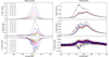 |
Fig. 3. Main pulse and interpulse of ten unnormalized average pulse profiles with different values of Ere. From top to bottom, the profiles correspond to I, L, and V. |
To investigate the profile variations in the main pulse more closely, the normalized average profiles of the ten groups are shown in the left panel of Fig. 4. The top-left panel shows that, with increasing relative energy, the total intensity of the main pulse exhibits a slight rightward drift in longitude and the pulse width gradually becomes narrower. The middle-left panel shows that the leading linear polarization components significantly decrease, suggesting that the relative polarization intensity of the leading components weakens with increasing relative energy, indicating a relationship between depolarization phenomena and flux intensity. The bottom-left panel shows that the circular polarization profile becomes narrower as Ere increases, but remains relatively stable compared to the total intensity and linear polarization.
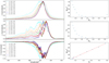 |
Fig. 4. Left three panels: Ten normalized average pulse profiles with different values of Ere in the main pulse, with I, L, and V displayed from top to bottom. Right three panels: Scatter plots of Ere-W10, Ere-FL, and FL-W10, respectively, with dashed red lines representing the results of the least squares linear fits. The uncertainties are very small and thus indistinguishable in the figure. |
The top and middle panels on the right side of Fig. 4 show the variations in W10 (the pulse width at 10% of the peak intensity) and FL of the main pulse, respectively, as functions of Ere, across the ten average profiles. Both W10 and FL initially decrease sharply as Ere increases, but begin to increase slowly once Ere reaches approximately 1.3. Given the similar variation trends of W10 and FL with Ere, their relationship is presented in the bottom panel on the right side of Fig. 4. For the first time, we identify a strong positive linear correlation between these parameters.
3.2. Orthogonal polarization modes
Figure 5 shows the PA curves from Profile 1 to Profile 10. In the longitude range 295–317°, PA jumps gradually begin to appear with increasing Ere, although the magnitude of the jumps remains relatively small. The bulge formed by the PA of the total average profile in Fig. 1 is caused by the PA jumps of pulses with relatively large Ere. Several nearly orthogonal PA jumps occur within the longitude range 265–285° in the PA curve of Profile 10. This indicates that PA jumps are related to the flux intensity of the pulse. Figure 6 presents the polarization information for Profile 10 and the total average profile; all profiles have been normalized by their peak values. In the leading edge region of the main pulse, approximately at longitudes 271° and 276°, the PA exhibits two distinct jumps. Furthermore, at the longitudes where the PA jumps occur, the linear polarization intensity drops sharply to nearly zero, confirming that depolarization occurs at these locations and possibly results from the superposition of two orthogonal polarization waves.
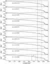 |
Fig. 5. PA curves corresponding to the ten average pulse profiles. The green line represents the PA curve corresponding to the total average pulse profile. From top to bottom, the Ere values gradually increase. The dashed black region in the last panel corresponds to the longitude range 265–285°. The dashed purple region indicates the longitude range 295–317°. |
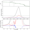 |
Fig. 6. Top panel: Black curve represents the PA curve of Profile 10, while the green curve represents the PA curve of the total average pulse profile. Middle panel: Solid black, red, and blue lines represent I, L, and V respectively, with the total average pulse profile (dotted line) shown as a reference background. Bottom panel: Enlarged view of the region enclosed by the two dashed horizontal lines in the middle panel. Dashed vertical lines in the top and bottom panels indicate the pulse longitude range 265–285°. |
The top panel of Fig. 7 shows the 2D statistical distribution of PA for all single pulses. The bottom panel shows the total average PA curve. The 2D statistical distribution of PA clearly reveals the presence of two polarization modes in this pulsar. In particular, within the two dashed black ellipses, a nearly 90° PA jump is visible. Therefore, the subsequent analysis focuses on the orthogonal polarization modes at longitudes I and II. The statistical distribution of single-pulse PA values at longitude I is shown in Fig. 8, with PA values corresponding to the range indicated by the dashed red lines in Fig. 7. Two Gaussian distributions are observed in the PA distribution at this location. Fitting these two Gaussian distributions yields a PA separation (△PA) of 87.86° at this position. The value of △PA is obtained from the difference between the peak positions of the two Gaussian functions. This indicates the presence of almost 90° orthogonal polarization modes at longitude I. In Fig. 8, we refer to the less populated PA distribution on the right side of the dashed purple line as the secondary mode (Mode S) of the orthogonal polarization states, while the more populated distribution on the left is referred to as the main mode (Mode M).
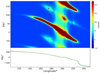 |
Fig. 7. Top panel: 2D statistical distribution of PA and PA ± 180° for all single pulses, showing only PA values within the main pulse region. The dashed black ellipse corresponds to the two areas where PA jumps occur most frequently, with black dots indicating the centers of these ellipses. The two dashed red lines mark the longitude positions of the black dots, labeled longitude I and II, respectively. The PA range for these two dashed red lines spans from the value of the black dots minus 135° to the value plus 45°. Bottom panel: Curve of the PA for the total average pulse profile. |
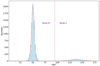 |
Fig. 8. Statistical distribution of the PA of single pulses at longitude I. The dashed red lines represent the result of fitting two Gaussian functions. The dashed purple vertical line indicates the midpoint between the peak positions of the Gaussian functions, with the areas on either side corresponding to the two modes, Mode M and Mode S. |
We obtained 958 single pulses at longitude I with PA in Mode S and plotted the corresponding average pulse profile in Fig. 9a. In the PA curve of the top panel, a nearly 90° PA jump occurs around longitudes 266° and 283°. The bottom panel shows that the shape of the linear polarization profile also changes, with depolarization occurring at the locations of the PA jumps. To investigate whether the flux intensity of these single pulses has changed, the probability density distribution of their Ere is plotted in Fig. 9b. The orange histogram represents the Ere distribution of all single pulses observed in this study, while the green histogram shows the Ere distribution of single pulses in Mode S at longitude I. From the two statistical distributions, the average relative energy of single pulses in Mode S at longitude I is higher than that of all single pulses. The difference becomes more pronounced when Ere is greater than 2. This finding is consistent with the significant PA jump observed for Profile 10 in the 265–285° longitude range in Fig. 5. This suggests that the single pulses in Mode S occur more frequently with stronger radiation energy, and that the orthogonal polarization modes are associated with the flux intensity of the pulses.
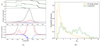 |
Fig. 9. (a) Top panel: PA curve of the total average pulse profile is represented by the green line, while the black line represents the PA curve of the average pulse profile folded from single pulses in Mode S at longitude I. Middle panel: Dotted lines represent the total average pulse profiles of I, L, and V, while the solid line represents the average pulse profile folded from the single pulses in Mode S at longitude I. (b) Statistical distribution of Ere: the orange color corresponds to all single pulses observed, while the green color corresponds to single pulses in Mode S at longitude I. |
Following the same procedure as described above, single pulses at longitude II were also analyzed. Figure 10 shows that the statistical distribution of single-pulse PA at longitude II also exhibits two components. A model consisting of a constant term and two Gaussian functions was used to fit the statistical distribution. The fit reveals a PA separation of 87.71° at longitude II, indicating the presence of a nearly 90° polarization mode at this location. However, the number of single pulses in Mode S at longitude II is significantly higher than at longitude I. We obtained a total of 4311 single pulses at longitude II, with the PA in Mode S. The average profile obtained by folding these single pulses in Mode S at Longitude II is shown in Fig. 11a. The top panels show that a PA jump occurs at approximately longitude 300°. Since the PA covers a relatively broad range at longitude II, the PA jump in the average pulse profile is less than 90°. The bottom panel shows that, at the location of the PA jump, depolarization occurs, but the linear polarization intensity does not decrease to zero. Figure 11b plots the Ere distribution of single pulses in Mode S at longitude II. The Ere distribution of these pulses is similar to that of all single pulses observed in this session. From these two statistical distributions, the average pulse energy of single pulses in Mode S is still slightly higher than that of all single pulses observed in this session. Within this longitude range, this finding is also consistent with the gradual PA jump observed in Fig. 5 as Ere increases.
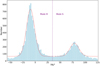 |
Fig. 10. Similar to Fig. 8, but for longitude II. The dashed red line is derived from a fit using a model consisting of a constant term and two Gaussian functions. |
3.3. Microstructure characteristics
In the single-pulse radiation of this pulsar, the total intensity exhibits abundant microstructure, which displays periodic characteristics. This study focused exclusively on the periodic microstructure within the main pulse region. The process of identifying microstructure was as follows. First, the longitude range corresponding to the main pulse was determined by applying a windowed filtering approach to the smoothed total average pulse profile. Because of the strong baseline radiation in this pulsar’s signal, a differencing operation was applied to the signal in the main pulse region to reduce the influence of the baseline radiation. The optimal order of differentiation was determined using the Akaike Information Criterion, with a maximum order of five. To reduce the influence of strong pulse components on the autocorrelation function (ACF), the differenced data were divided into three equal parts. The pulse signal in each part was processed using the ACF. The ACF was defined as follows:
 (2)
(2)
Generally, in the ACF, the first dip is designated as the width of the microstructure (tμ), while the first peak is designated as the period of microstructure (Pμ; Mitra et al. 2015). To ensure the reliability of the identified periodic microstructure, additional processing was applied to the ACF. First, cubic spline interpolation was performed on the ACF. Using a peak-finding function, the first dip, the first peak, the second peak, and the third peak were identified in the ACF interpolated with a spline. If the second and third peak positions deviate by less than 20% from their theoretical positions (twice or three times the first peak position), the signal can be considered a sequence of periodic microstructure (Kramer et al. 2024). Additionally, the power spectral density (PSD) of the differenced data and the ACF were calculated. The PSD helps identify abnormally high-frequency signals and eliminates the misidentification of microstructure caused by periodic noise signals. The main pulse of the total average pulse profile was divided into three fixed windows, and all analyses of single-pulse microstructure were performed within these predefined windows.
Figure 12 presents an example of periodic microstructure. Differencing effectively removes the influence of baseline radiation, allowing microstructure previously masked by the baseline radiation to become clearly visible. Both the ACF and PSD images show that the identified microstructure exhibits strong periodicity. The PSD image of the differenced signal and that of the ACF exhibit the same characteristic frequencies, indicating that the selected periodic microstructure is reliable.
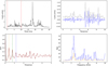 |
Fig. 12. Example of the microstructure of PSR B0950+08. Top-left panel: Total intensity of a single pulse in the main pulse region; the dashed red area marks the window size of the first third of the main pulse. Top-right panel: Microstructure that satisfies the condition, corresponding to the dashed red region in the top-left panel. The gray and blue lines show the original data of the total intensity and the result after differencing, respectively. Bottom-left panel: ACF of the differenced signal; the solid black line is the initial ACF and the dashed red line represents the cubic spline interpolation of the ACF. Dashed black, orange, green, and blue vertical lines correspond to the first dip and the first, second, and third peaks in the spline-interpolated ACF, respectively. Bottom-right panel: Solid blue line represents the PSD of the differenced signal and the solid orange line represents the PSD of the ACF. |
Using this method, we performed a microstructure search on the total intensity of 14 231 single pulses in the main pulse region, yielding 7840 periodic microstructure samples. We calculated tμ and Pμ for the identified microstructure. Figure 13 shows the statistical distributions of tμ and Pμ. The median of each distribution was taken as the final result for each, and the median absolute deviation was used to quantify the uncertainties. Ultimately, we obtained  and Pμ = 221 ± 59(μs)) for PSR B0950+08.
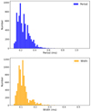 |
Fig. 13. Statistical distribution of the microstructure width tμ and period Pμ for PSR B0950+08 in the main pulse region. |
4. Discussion
From the ten unnormalized average pulse profiles in Fig. 3, the total intensity of the main pulse shows significant variation as Ere increases, whereas the total intensity of the interpulse, except for Profile 10, remains relatively stable. This reflects a decreasing intensity ratio between the interpulse and the main pulse as Ere increases, indicating that the intensity variation of the main pulse is larger than that of the interpulse. This suggests that the interpulse and the main pulse may have different radiation properties. For the linear polarization intensity, the main pulse intensity and shape exhibit significant variation across the ten profiles. In general, the variation in the interpulse of linear polarization with increasing Ere is less significant, compared to the main pulse. In the circular polarization profiles, we observed the change in circular polarization sign in the interpulse of Profile 10. However, this sign change is not seen in the total average pulse profile due to masking by the folding process of the single pulses. This suggests that changes in circular polarization sign occur more frequently in strong pulses.
Figure 4 shows that as Ere increases, the position of the main pulse in the total intensity gradually shifts to the right. The W10 of the main pulse in the total intensity decreases with increasing Ere, then slowly increases. This indicates that as the flux intensity increases, the width of the main pulse initially narrows sharply and then gradually widens. Regarding the linear polarization intensity, as Ere increases, the leading edge components of the main pulse gradually disappear and a more pronounced depolarization phenomenon emerges. Therefore, as Ere increases, FL exhibits the same trend as W10, and there is a strong linear correlation between FL and W10.
The evolution of the PA curve with increasing Ere reveals that the main pulse exhibits subtle yet progressively larger PA jumps. Multiple PA jumps of approximately 90° abruptly appear near the leading edge of the main pulse in Profile 10. Depolarization consistently occurs at the locations of PA jumps. Therefore, both depolarization and PA jumps are modulated by the flux intensity.
The number of single pulses in Mode S is smaller than that in Mode M, and the folding process obscures the PA jump characteristics of single pulses. Consequently, no significant PA jumps are observed in the main pulse region of the total average PA curve. In the PA distribution of all single pulses observed, two distinct polarization modes appear at both longitude I and longitude II, separated by approximately 90°. Profile 10 exhibits multiple PA jumps in the longitude range 265–285°, which corresponds to the orthogonal polarization modes at longitude I shown in Fig. 7. Furthermore, the single pulses in Mode S at longitude I also exhibit relatively strong energy, suggesting that these single pulses in Mode S are likely among the stronger individual pulses. At longitude II, the average relative energy of single pulses in Mode S is slightly stronger than that of all single pulses observed in this study. The PA distribution at longitude II is more complex, with a broader range of PA jump regions. In addition to the orthogonal polarization modes, more intricate polarization modes are also present. Therefore, we conclude that phenomena such as changes in the circular polarization sign, PA jumps, and depolarization are correlated with the flux intensity of the pulsar. The stronger the pulse radiation, the more pronounced these phenomena become.
For the periodic microstructure, we obtained the width of the microstructure for the total intensity of tμ = 110 ± 20(μs), which is consistent with tμ(s) ≈ (0.43±0.079) × 10−3P(s), in agreement with the relationship identified by Cordes (1979) between tμ and the rotation period of the pulsar. Furthermore, our result is consistent with the relation tμ(μs) = (600±100)P(s)1.1 ± 0.2 derived by Kramer et al. (2002) through the observational results of different pulsars. Because our statistical results support a linear relationship between microstructure width and rotation period, the microstructure is likely formed by a narrow radiation beam that sweeps across the line of sight. This suggests that the origin of the microstructure width is related to the angular width of the emission beam. Table 1 summarizes tμ values previously reported for PSR B0950+08 alongside our results at different frequencies. The table shows that the previous results for PSR B0950+08 generally align with this theoretical relationship. Figure 14 presents our results and those of other researchers on the periodic microstructure width in this pulsar. We find a positive correlation between tμ and the observational frequency. Due to the large uncertainties in these data, it is still uncertain whether the same conclusion applies to other pulsars.
Results of the periodic microstructure width for PSR B0950+08 from previous studies and this work.
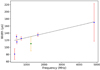 |
Fig. 14. Relationship between periodic microstructure width tμ of PSR B0950+08 and observational frequency. Data include results from previous studies and our own calculations listed in Table 1. Blue dots indicate literature values, while the green diamond represents our calculation. The dashed black line indicates the result of a linear fit. |
5. Summary
In this study, we classified single pulses of PSR B0950+08 into ten groups according to their flux intensity and plotted their corresponding average pulse profiles. Analysis of these normalized average profiles reveals that the main pulse in total intensity shifts to the right as Ere increases. Additionally, there is a trend where W10 of the main pulse initially decreases sharply and then increases slowly with Ere. For the linear polarization intensity, as Ere increases, the leading components of the main pulse disappear, resulting in a decrease in the relative linear polarization intensity. As a result, FL exhibits a trend similar to W10 as Ere increases, and there is also a strong linear relationship between FL and W10.
For Profile 10, we observed multiple jumps in the PA around longitudes 265–285°, as well as several reversals in the circular polarization sign. The statistical distribution of the single-pulse PA confirms that there are indeed two orthogonal polarization modes at longitudes I and II. The single pulses in Mode S at longitude I generally exhibit higher energy. These findings suggest that these peculiar polarization behaviors are likely associated with the intensity of the pulse radiation.
This pulsar exhibits a significant amount of microstructure, and we identified and filtered the microstructure within the main pulse region from all single pulses. We obtained tμ = 110 ± 20(μs) and Pμ = 221 ± 59(μs), consistent with the empirical formula proposed by previous researchers.
The FAST data policy and instructions on how to request public data can be found online: https://fast.bao.ac.cn
Acknowledgments
This work was supported by the National Natural Science Foundation of China (NSFC) under No.12133004. This work utilizes the public data from the FAST, a national large-scale facility in China, which is built and operated by the National Astronomical Observatories, Chinese Academy of Sciences (NAOC). We would like to thank the staff at the NAOC for making these observations possible.
References
- Bilous, A. V., Grießmeier, J. M., Pennucci, T., et al. 2022, A&A, 658, A143 [NASA ADS] [CrossRef] [EDP Sciences] [Google Scholar]
- Cordes, J. M. 1979, Aust. J. Phys., 32, 9 [NASA ADS] [CrossRef] [Google Scholar]
- Cordes, J. M., Kramer, M., Lazio, T. J. W., et al. 2004, New Astron. Rev., 48, 1413 [CrossRef] [Google Scholar]
- Craft, H. D., Comella, J. M., & Drake, F. D. 1968, Nature, 218, 1122 [Google Scholar]
- Everett, J. E., & Weisberg, J. M. 2001, ApJ, 553, 341 [NASA ADS] [CrossRef] [Google Scholar]
- Gould, D. M., & Lyne, A. G. 1998, MNRAS, 301, 235 [NASA ADS] [CrossRef] [Google Scholar]
- Hankins, T. H. 1996, in IAU Colloq. 160: Pulsars: Problems and Progress, eds. S. Johnston, M. A. Walker, & M. Bailes, ASP Conf. Ser., 105, 197 [Google Scholar]
- Hankins, T. H., & Boriakoff, V. 1978, Nature, 276, 45 [CrossRef] [Google Scholar]
- Hankins, T. H., & Boriakoff, V. 1981, ApJ, 249, 238 [Google Scholar]
- Hankins, T. H., & Cordes, J. M. 1981, ApJ, 249, 241 [NASA ADS] [CrossRef] [Google Scholar]
- Hankins, T. H., Izvekova, V. A., Malofeev, V. M., et al. 1991, ApJ, 373, L17 [Google Scholar]
- Hobbs, G., Lyne, A. G., Kramer, M., Martin, C. E., & Jordan, C. 2004, MNRAS, 353, 1311 [NASA ADS] [CrossRef] [Google Scholar]
- Hotan, A. W., van Straten, W., & Manchester, R. N. 2004, PASA, 21, 302 [Google Scholar]
- Jiang, P., Yue, Y., Gan, H., et al. 2019, Sci. China: Phys. Mech. Astron., 62, 959502 [Google Scholar]
- Kramer, M., Johnston, S., & van Straten, W. 2002, MNRAS, 334, 523 [Google Scholar]
- Kramer, M., Liu, K., Desvignes, G., Karuppusamy, R., & Stappers, B. W. 2024, Nat. Astron., 8, 230 [Google Scholar]
- Kuzmin, A. D., Izvekova, V. A., Shitov, Y. P., et al. 1998, A&AS, 127, 355 [NASA ADS] [CrossRef] [EDP Sciences] [Google Scholar]
- Lange, C., Kramer, M., Wielebinski, R., & Jessner, A. 1998, A&A, 332, 111 [NASA ADS] [Google Scholar]
- Manchester, R. N., Taylor, J. H., & Huguenin, G. R. 1975, ApJ, 196, 83 [NASA ADS] [CrossRef] [Google Scholar]
- Mitra, D., Arjunwadkar, M., & Rankin, J. M. 2015, ApJ, 806, 236 [NASA ADS] [CrossRef] [Google Scholar]
- Popov, M. V., Bartel, N., Cannon, W. H., et al. 2002, A&A, 396, 171 [NASA ADS] [CrossRef] [EDP Sciences] [Google Scholar]
- Radhakrishnan, V., & Cooke, D. J. 1969, Astrophys. Lett., 3, 225 [NASA ADS] [Google Scholar]
- Singh, S., Gupta, Y., & De, K. 2024, MNRAS, 527, 2612 [Google Scholar]
- Stinebring, D. R., Cordes, J. M., Rankin, J. M., Weisberg, J. M., & Boriakoff, V. 1984, ApJS, 55, 247 [NASA ADS] [CrossRef] [Google Scholar]
- Stovall, K., Ray, P. S., Blythe, J., et al. 2015, ApJ, 808, 156 [NASA ADS] [CrossRef] [Google Scholar]
- Ul’yanov, O. M., & Zakharenko, V. V. 2012, Astron. Rep., 56, 417 [Google Scholar]
- Ulyanov, O. M., Skoryk, A. O., Shevtsova, A. I., Plakhov, M. S., & Ulyanova, O. O. 2016, MNRAS, 455, 150 [NASA ADS] [CrossRef] [Google Scholar]
- van Straten, W., Demorest, P., & Oslowski, S. 2012, Astron. Res. Technol., 9, 237 [NASA ADS] [Google Scholar]
- Wang, Z., Lu, J., Jiang, J., et al. 2022, MNRAS, 517, 5560 [NASA ADS] [CrossRef] [Google Scholar]
- Xie, J., Wang, J., Wang, N., et al. 2022, ApJ, 940, L21 [NASA ADS] [CrossRef] [Google Scholar]
- Yao, J. M., Manchester, R. N., & Wang, N. 2017, ApJ, 835, 29 [NASA ADS] [CrossRef] [Google Scholar]
All Tables
Results of the periodic microstructure width for PSR B0950+08 from previous studies and this work.
All Figures
|
Fig. 1. Total average pulse profile of PSR B0950+08. The top panel shows the PA curve of the total average pulse profile with σψ < 5°, along with the curve of PA ± 180°. To facilitate analysis of PA properties, the green curve representing the continuous variation of PA is plotted. The middle panel displays the average pulse profiles of total intensity I (solid black line), linear polarization L (solid red line) and circular polarization V (solid blue line), respectively. The zoom-in box shows the noise level region. The bottom panel presents a zoomed-in view of the region as outlined by the dashed box in the middle panel. The zoomed-in view of the circular polarization of the interpulse is shown within the rectangular box in the bottom panel. |
| In the text | |
|
Fig. 2. Statistical distribution of Ere for 14 231 single pulses. |
| In the text | |
|
Fig. 3. Main pulse and interpulse of ten unnormalized average pulse profiles with different values of Ere. From top to bottom, the profiles correspond to I, L, and V. |
| In the text | |
|
Fig. 4. Left three panels: Ten normalized average pulse profiles with different values of Ere in the main pulse, with I, L, and V displayed from top to bottom. Right three panels: Scatter plots of Ere-W10, Ere-FL, and FL-W10, respectively, with dashed red lines representing the results of the least squares linear fits. The uncertainties are very small and thus indistinguishable in the figure. |
| In the text | |
|
Fig. 5. PA curves corresponding to the ten average pulse profiles. The green line represents the PA curve corresponding to the total average pulse profile. From top to bottom, the Ere values gradually increase. The dashed black region in the last panel corresponds to the longitude range 265–285°. The dashed purple region indicates the longitude range 295–317°. |
| In the text | |
|
Fig. 6. Top panel: Black curve represents the PA curve of Profile 10, while the green curve represents the PA curve of the total average pulse profile. Middle panel: Solid black, red, and blue lines represent I, L, and V respectively, with the total average pulse profile (dotted line) shown as a reference background. Bottom panel: Enlarged view of the region enclosed by the two dashed horizontal lines in the middle panel. Dashed vertical lines in the top and bottom panels indicate the pulse longitude range 265–285°. |
| In the text | |
|
Fig. 7. Top panel: 2D statistical distribution of PA and PA ± 180° for all single pulses, showing only PA values within the main pulse region. The dashed black ellipse corresponds to the two areas where PA jumps occur most frequently, with black dots indicating the centers of these ellipses. The two dashed red lines mark the longitude positions of the black dots, labeled longitude I and II, respectively. The PA range for these two dashed red lines spans from the value of the black dots minus 135° to the value plus 45°. Bottom panel: Curve of the PA for the total average pulse profile. |
| In the text | |
|
Fig. 8. Statistical distribution of the PA of single pulses at longitude I. The dashed red lines represent the result of fitting two Gaussian functions. The dashed purple vertical line indicates the midpoint between the peak positions of the Gaussian functions, with the areas on either side corresponding to the two modes, Mode M and Mode S. |
| In the text | |
|
Fig. 9. (a) Top panel: PA curve of the total average pulse profile is represented by the green line, while the black line represents the PA curve of the average pulse profile folded from single pulses in Mode S at longitude I. Middle panel: Dotted lines represent the total average pulse profiles of I, L, and V, while the solid line represents the average pulse profile folded from the single pulses in Mode S at longitude I. (b) Statistical distribution of Ere: the orange color corresponds to all single pulses observed, while the green color corresponds to single pulses in Mode S at longitude I. |
| In the text | |
|
Fig. 10. Similar to Fig. 8, but for longitude II. The dashed red line is derived from a fit using a model consisting of a constant term and two Gaussian functions. |
| In the text | |
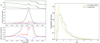 |
Fig. 11. Same as Fig. 9, but for longitude II. |
| In the text | |
|
Fig. 12. Example of the microstructure of PSR B0950+08. Top-left panel: Total intensity of a single pulse in the main pulse region; the dashed red area marks the window size of the first third of the main pulse. Top-right panel: Microstructure that satisfies the condition, corresponding to the dashed red region in the top-left panel. The gray and blue lines show the original data of the total intensity and the result after differencing, respectively. Bottom-left panel: ACF of the differenced signal; the solid black line is the initial ACF and the dashed red line represents the cubic spline interpolation of the ACF. Dashed black, orange, green, and blue vertical lines correspond to the first dip and the first, second, and third peaks in the spline-interpolated ACF, respectively. Bottom-right panel: Solid blue line represents the PSD of the differenced signal and the solid orange line represents the PSD of the ACF. |
| In the text | |
|
Fig. 13. Statistical distribution of the microstructure width tμ and period Pμ for PSR B0950+08 in the main pulse region. |
| In the text | |
|
Fig. 14. Relationship between periodic microstructure width tμ of PSR B0950+08 and observational frequency. Data include results from previous studies and our own calculations listed in Table 1. Blue dots indicate literature values, while the green diamond represents our calculation. The dashed black line indicates the result of a linear fit. |
| In the text | |
Current usage metrics show cumulative count of Article Views (full-text article views including HTML views, PDF and ePub downloads, according to the available data) and Abstracts Views on Vision4Press platform.
Data correspond to usage on the plateform after 2015. The current usage metrics is available 48-96 hours after online publication and is updated daily on week days.
Initial download of the metrics may take a while.