| Issue |
A&A
Volume 701, September 2025
|
|
|---|---|---|
| Article Number | A68 | |
| Number of page(s) | 15 | |
| Section | Extragalactic astronomy | |
| DOI | https://doi.org/10.1051/0004-6361/202554813 | |
| Published online | 03 September 2025 | |
Observation of the spectral turnover in the afterglow emission of GRB 221009A
1
Gran Sasso Science Institute, Viale F. Crispi 7, L’Aquila (AQ) I-67100, Italy
2
INFN – Laboratori Nazionali del Gran Sasso L’Aquila (AQ) I-67100, Italy
3
Ioffe Institute, 26 Politekhnicheskaya, St Petersburg 194021, Russia
4
Department of Physics, University of Cagliari, SP Monserrato-Sestu, Cagliari, 09042 Cagliari, Italy
⋆ Corresponding authors: This email address is being protected from spambots. You need JavaScript enabled to view it.
, This email address is being protected from spambots. You need JavaScript enabled to view it.
, This email address is being protected from spambots. You need JavaScript enabled to view it.
Received:
27
March
2025
Accepted:
30
June
2025
Abstract
The afterglow emission of gamma-ray bursts (GRBs) originates from deceleration of the ultra-relativistic matter in the circumburst medium. Observations of afterglow in the high-energy and very high-energy domains provide essential information about the physics of acceleration in relativistic shocks. The lack of sensitivity in the mega-electronvolt gamma rays in the afterglow phase prevents us from constraining the spectral turnover from the X-ray to tera-electronvolt energies. GRB 221009A offers the unique opportunity to characterize spectral components during the prompt and early afterglow phases and probe their origin, including mega-electronvolt observations. Analyzing the multiwave band afterglow emission, we identified two distinct spectral components during the initial 30 minutes. The second spectral component peaks at ∼100 GeV, and the bolometric fluence (10 MeV–10 TeV) is greater than 2 × 10⁻³ erg/cm2. Performing broadband spectral modeling, we provide constraints on the magnetic field (∼0.1 G) and the energies of the accelerated electrons in the external relativistic shock.
Key words: astroparticle physics / radiation mechanisms: non-thermal / relativistic processes / methods: observational / gamma-ray burst: general / stars: jets
© The Authors 2025
 Open Access article, published by EDP Sciences, under the terms of the Creative Commons Attribution License (https://creativecommons.org/licenses/by/4.0), which permits unrestricted use, distribution, and reproduction in any medium, provided the original work is properly cited.
This article is published in open access under the Subscribe to Open model. This email address is being protected from spambots. You need JavaScript enabled to view it. to support open access publication.
1. Introduction
Gamma-ray bursts (GRBs) are extragalactic transients that are detected as brief mega-electronvolt flashes of seconds to minutes in duration (prompt emission). This radiation is produced in the ultra-relativistic jets formed right after the death of a particular class of massive stars or a merger of neutron stars. The brief prompt emission phase is followed by days-long afterglow radiation. The afterglow emission is produced due to the deceleration of the GRB jet in the circumburst medium (Paczynski & Rhoads 1993; Mészáros & Rees 1997; Sari et al. 1998). The expansion of the GRB ejecta in the surrounding medium forms an external relativistic shock. Once the medium particles are accelerated in the shock, they lose their energy via synchrotron and inverse Compton radiation (Sari & Esin 2001). For the last 20 years the afterglow emission has been extensively studied, from radio wavelengths to high-energy (HE) gamma rays. The multiwavelength emission up to giga-electronvolt gamma rays has been interpreted as due to the synchrotron radiation from the nonthermal electron population accelerated in the relativistic shock. However, capturing only the properties of the synchrotron spectrum of the afterglows does not allow one to break the degeneracies between the microphysical parameters of the shock as well as the profile of the circumburst medium and the injected kinetic power. Observations of the second, very high-energy (VHE) spectral component are essential, then, for constraining the fundamental microphysical parameters of the shock. In the past, most HE (> 100 MeV) observations of GRB afterglows have indicated that the giga-electronvolt photons originate from the synchrotron part of the spectrum, with some exceptions (see Nava 2018 for a review).
In 2019, the two Imaging Atmospheric Cherenkov Telescopes (IACTs), Major Atmospheric Gamma-ray Cherenkov Telescopes (MAGIC), and the High Energy Stereoscopic System (H.E.S.S.) discovered tera-electronvolt emission from a GRB. GRB 190114C (MAGIC Collaboration 2019; Veres et al. 2019), located at redshift z = 0.46, was detected by MAGIC approximately 62 s after the Gamma ray Burst Monitor on board the Fermi satellite (Fermi/GBM) trigger time. This pivotal observation of GRB 190114C enabled an analysis of the time-resolved VHE gamma-ray (VHE; E > 100 GeV) spectrum across multiple epochs, extending well beyond 2000 s. Spectral analysis, using concurrent data, was reported to be consistent with synchrotron self-Compton (SSC) radiation (Veres et al. 2019) from the electrons accelerated in the forward shock (see Miceli & Nava 2022 for a review). The H.E.S.S. collaboration detected the VHE emission of GRB 180720B at redshift z = 0.653 (Abdalla et al. 2019) occurring 10 ks after the Fermi/GBM trigger time. Later, H.E.S.S. also detected GRB 190829A (Abdalla et al. 2021). This observation was used to perform a joint spectral analysis with Swift/XRT during two time periods: after about (1) 4–8 h and (2) 27–32 h. The joint analysis reveals that a single emission component could in principle account for the broadband spectra. A separate study by Salafia et al. (2022) has shown that SSC model is capable of producing the observed spectral energy distribution (SED) for this GRB.
Several other GRBs, including GRB 201216C (Abe et al. 2023; Nava 2021), have been discovered (detection significance above 5σ) by IACTs to date. We provide a summary of the available multiwavelength data recorded during VHE observations of GRB afterglows in Table 1.
Multiwavelength observation of GRBs discovered by IACTs since 2018.
The afterglow emission is frequently observed in soft X-rays alongside tera-electronvolt gamma rays. However, the data in the hard X-rays and mega-electronvolt–giga-electronvolt gamma rays remain weakly constrained. For GRB 190114C, the discovery of a secondary VHE spectral component beyond the mega-electronvolt spectrum was claimed (MAGIC Collaboration 2019), thanks to the detection of rather fainter giga-electronvolt emissions. To observe the turnover in the spectrum from low-energy synchrotron radiation to HE spectral components such as SSC in GRB afterglows, more sensitive measurements in the hard X-rays to giga-electronvolt energies arecrucial.
On October 9, 2022, GRB 221009A was detected by both ground-based and space-borne observatories and subsequently identified as one of the most energetic bursts on record (Lesage et al. 2023; Frederiks et al. 2023) at redshift 0.15 (Malesani et al. 2025). This intense burst was observed during its initial emission phase by Fermi/GBM and Konus-Wind (KW), leading to its identification as having the highest prompt fluence and peak flux (Lesage et al. 2023; Frederiks et al. 2023; Burns et al. 2023). The intense fluence saturated the GBM during specific phases, termed bad time intervals (BTIs), BTI-1: 218.5–277.9 s and BTI-2: 507.3–514.4 s after the GBM trigger time, which were marked as unusable intervals for the data analysis (Lesage et al. 2023). During the initial phase up to 247 s, around the peak of the brightest pulse, only KW was able to recover the prompt-emission spectrum of GRB 221009A (Frederiks et al. 2023). Most interestingly, LHAASO observed GRB 221009A (Cao et al. 2023) starting from the onset of the burst, thanks to its wide field of view (FoV) and high duty cycle (Cao et al. 2024). The time-resolved spectral analysis covering the energy band 0.3–5 TeV revealed a VHE emission up to approximately one hour after the trigger. In this study, we consider the observation periods of LHAASO as reference time bins. Several authors have investigated the multiwavelength afterglow emission at late epochs (hours after the GRB trigger) and discussed the effects of the jet structure (O’Connor et al. 2023; Sato et al. 2023; Fraija et al. 2024; Laskar et al. 2023; Ren et al. 2024), the radiation from the reverse shock (Bright et al. 2023; Laskar et al. 2023), and the frequency-dependent growth of the apparent size of the afterglow emission region (Giarratana 2024). We focus on the early (first ∼20 min) kilo-electronvolt–tera-electronvolt spectra of GRB 221009A. Previous studies of early giga-electronvolt–tera-electronvolt radiation from GRB 221009A were limited to the investigation of temporal properties (Zhang et al. 2023a; Ren et al. 2024) or joint giga-electronvolt–tera-electronvolt spectra with the piled-up data of Fermi/LAT (240–248 s in Wang et al. 2023) or the giga-electronvolt data in the off-source position of the Fermi/LAT (326–900 s in Wang et al. 2023).
This article is organized as follows. Section 2 outlines the data analysis techniques used, including data reduction methods from previous studies. In Section 3, we explore the temporal and spectral analysis of the GRB. Section 4 addresses the potential origins of the giga-electronvolt–tera-electronvolt component, and the main findings are summarized in Section 5.
2. Multiwavelength data
The available period of instrument coverage from X-rays (kilo-electronvolt) to tera-electronvolt energies is reported in Figure 1 and Table 2.
 |
Fig. 1. Illustration of the data availability in each time bin (time stamps indicated in the vertical axis on the left and numbered bins on the right) for each instrument (see Table 2). Areas marked with slashes indicate bins impacted by pile-up in both Fermi/GBM and Fermi/LAT. A simple double-hump spectrum is shown to indicate the preliminary peak positions of the two components seen in GRB 221009A. The selection of time bins is based on the presence of multiwavelength data spanning kilo-electronvolt to tera-electronvolt energies. Six bins (BIN-2, −6, −7, −8, −12, and −14) were chosen for time-resolved spectral analysis. |
Coverage of GRB 221009A by multiwavelength instruments.
2.1. LHAASO
GRB 221009A was observed in the LHAASO field for more than 30 minutes after the initial trigger by Fermi/GBM. The detection count surpassed 64 000 photons with energies greater than 200 GeV. The peak emission was observed around 240 s after the trigger. The observed VHE gamma-ray emission is identified as an afterglow. Spectral data, as is shown in Table 3, were adapted from Cao et al. (2023). The LHAASO time intervals in the table are used as references for our analyses adding simultaneous (or quasi-simultaneous) data from Fermi/LAT or AGILE. The information presented in Table 3 includes both the flux and the intrinsic spectral index of the source, corrected for extragalactic background suppression (Cao et al. 2023). The intrinsic spectral index for VHE gamma rays in the energy band of 0.3–5 TeV is between 2.2 and 2.4, while the flux varies by two orders of magnitude (10−5–10−7 erg cm−2 s−1). Although the maximum energy photon from GRB 221009A is reported to be about 10 TeV (The LHAASO Collaboration 2023), energies above 5 TeV are not considered, as they do not affect the results of this study. The (finely binned) gamma-ray flux of VHE (Figure 3A1) was obtained from LHAASO, as is detailed in Cao et al. (2023), together with the intrinsic spectral indices (course-binned; Figure 3B2). These reported flux and spectral indices in Figure 3 from Cao et al. (2023) have been corrected for extragalactic background light (EBL) and represent the intrinsic parameters of the source. The fluxes in the broad temporal bins, the same bins for which the spectral indices are reported, are not documented in Cao et al. (2023). Therefore, we rebinned the flux into the bin where the spectral information is available (utilizing the data from Figure 3A1) and applied a zeroth-order polynomial fit. This rebinning of the flux provides the intrinsic flux of the source in the temporal bins where the spectral index is reported. As is noted in Cao et al. (2023), the published fluxes exclude the systematic uncertainty of 10.7%. In the rebinning analysis stated above, we incorporate this 10.7% systematic uncertainty together with the statistical uncertainty of the fit, in quadrature. The results of this rebinning are reported in Figure 2 and Table 3.
Intrinsic spectral parameters for LHAASO.
 |
Fig. 2. Energy flux observed with LHAASO extracted from publicly available data (Cao et al. 2023) for the periods reported with spectral index. In the analyzed time segments (named time bins: see Table 2) the light curve of LHAASO has been fit with a constant (pol-0) that represents the flux of GRB 221009A for that period. The blue markers in the top panel report the rebinned LHAASO flux for each period. The bottom panel reports the intrinsic spectral index observed with only LHAASO. |
2.2. Fermi/LAT
We used GTBURST software from the official Fermi-tools to extract and analyze the GRB 221009A data. The HE data were extracted in the energy band of 0.1–100 GeV from the region of interest (ROI) of 12° around the source location of RA = 288.28° and Dec = 19.49° (Fermi LAT Team 2022). The trigger by Fermi/GBM on October 9, 2022, at 13:16:59.988 UTC (equivalent to 687014225 s MET) is considered the trigger time (T0). Considering that the source was bright, we have not considered any source off-axis angle (θ) cut to clean the data. In addition, a zenith angle cut of 100° was applied to reduce the contamination of the gamma-ray photons from the Earth limb. A spectral model of type “powerlaw2” is considered for the analysis throughout along with the “isotr_template” and “template (fixed norm.)” for the particle background and the Galactic component, respectively. For the selected time bins, an “unbinned likelihood analysis” was performed. Flux and flux errors were estimated if the minimum test statistic (TSmin) is greater than 25, indicating a detection significance of more than 5σ, where the significance of the detection is given by  (Ajello et al. 2019). The selection of the instrument response function was made based on the duration. We used the response function “P8R3_TRANSIENT010E_V2” until 400 s from the trigger time following the analysis methods described in Ajello et al. (2019), Bissaldi et al. (2023). No Fermi/LAT LLE data are publicly available for this burst. We generated Fermi/LAT data products through GTBURST using the Standard ScienceTool3 and pipeline gtbin. In addition, we produced background counts and response files using gtbkg and gtrspgen, respectively (for example Ajello et al. 2020). The spectral files were produced in six energy bins between 100 MeV and 100 GeV. We fit the Fermi/LAT spectrum on XSPEC using Cash statistics. Following the recommendation of the Fermi/LAT collaboration (Bissaldi et al. 2023), we have considered an energy threshold of 125 MeV for BIN-2 (2444 –247 s) and BIN-3 (247–253 s). The spectral data points obtained for each time bin are consistent with the results from the standard likelihood analysis.
2.3. AGILE
Based on the operational status of the detectors (MCAL, RM, and GRID) on board AGILE, detailed in Table 1 in Tavani et al. (2023), we have identified specific temporal bins that align with selected temporal bins presented in Table 2: bin-c1: 273.0–303.0 s; bin-c2: 303.0–383.0 s; bin-d: 684.0–834.0 s; and bin-e: 1129.0–1279.0 s. These bins correspond to our chosen bins: BIN-6; BIN-7; BIN-8; BIN-12; and BIN-14 (see Figure 1 and Table 2 for details). For BIN-7 and BIN-8, the Fermi/LAT data were used, since AGILE data for these bins covered a longer period of 303.0–383.0 s (bin-c2), and hence the spectra information is not publicly available for shorter exposures.
2.4. Fermi/GBM
Given the unprecedented duration of this burst, the response matrices directly provided by the Fermi GBM Burst catalog5 do not cover all the emission, limiting the analysis up to ∼460 s from the burst trigger. In order to analyze time bins at later times, we generated response matrices using the GBM Response Generator6. This official Fermi tool allows for the creation of GBM response matrices out of GBM daily data for a burst at a given location and arbitrary time. We downloaded the daily data associated with October 9, 2022, from the Fermi GBM Daily Data online repository7.
We produced response files for the NaI 4, NaI 8, BGO 0, and BGO 1 detectors for a source at the location (RA = 288.26° and Dec = 19.77°, provided by Swift/XRT observations) between 400 s and 1800 s after the GBM trigger. For each time bin before 400 s, we produced weighted response files from the response matrices provided by the Fermi GBM catalog, whereas we used the custom-made response matrices for any time bin after 400 s. Once the GBM data were reduced, we performed spectral fits on all the selected time bins. For the fitting process, we used PYXSPEC8, the Python interface to the XSPEC spectral fitting program. We implemented a Python-based Bayesian X-ray analysis (BXA; Buchner 2016), which enables Bayesian parameter estimation and model comparison through nested sampling algorithms in PYXSPEC. We ignored the energy channels outside 40–900 keV for the NaI detectors. We selected the energy range 400 keV–40 MeV for the BGO data. Note that we ignored the data of BGO for the BIN-14, as it is consistent with the estimated background spectrum.
2.5. GBM background considerations
Given that the mega-electronvolt emission of GRB 221009A lasts more than 1000 s, using a lower-order polynomial (polynomial of order 2–3) to model the mega-electronvolt background is ineffective. This ineffectiveness is due to the significant variations in the mega-electronvolt background throughout the GRB duration. Furthermore, the components that influence the background exposed to the detector exhibit considerable fluctuations over these periods (Biltzinger et al. 2020). Accurate modeling of the background for such an extended duration requires the use of higher-order polynomials, which, however, raises the risk of data overfitting. A different method of estimating the background was originally introduced by Fitzpatrick et al. (2011) via the Fermi orbital subtraction (OSV) tool.
The GBM background radiation exposure varies in terms of position and orientation, as the satellite oscillates every two orbits, covering the full sky over 30 orbits. By calculating the average rates from 30 orbits prior and subsequent, we derived a background estimate for the desired time. Using the background intervals specified in Lesage et al. (2023) for a polynomial fit, we evaluated these methodologies. As is described in the top panel of Figure 3, the polynomial fit tends to underestimate the background compared to the estimation of the OSV tool. Consequently, in the range of 600–800 s (BIN-12 from Table 3), a traditional analysis (prescribed in Lesage et al. 2023) tends to overestimate the mega-electronvolt signal due to inaccurate background calculations. In this range, the polynomial fit gives around ∼6000 excess counts, while the OSV tool estimates an excess of ∼2000 (see Figure 3, right panel). The sensitivity of the polynomial fit to the chosen background region likely explains this discrepancy.
 |
Fig. 3. Comparison of the backgrounds above 1 MeV estimated with the OSV tool and the polynomial fit for GRB 221009A. The top panel represents the light curve above 1 MeV. The OSV background uses Poisson uncertainty for each bin, which is omitted graphically for visual clarity. |
The intervals for the background chosen by Lesage et al. (2023) are (–150, –10) and (1625, 2400) seconds with respect to the trigger time. In the analysis presented in our work, we have used the following time periods for background selection: (–150, –10) and (1500, 2000) seconds. We considered a set of parameters closer to the true signal, taking into account that the Earth occludes the source after 1470 s. This polynomial fit predicts a higher background than the OSV tool, as is shown in Figure 4. Since the OSV tool exhibits less sensitivity to background region selection compared to polynomial fitting, it presents a reliable alternative for estimating backgrounds in long-duration (∼ks) events. The development of the OSV pipeline used in this work utilizes the foundational tools outlined in Fitzpatrick et al. (2011). In order to adapt to the requirements, certain components of the code have been modified. The primary changes involve migrating from Python 2 to Python 3. The complete code is available at the following link9 (De Santis 2024).
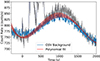 |
Fig. 4. Light curve of GRB 221009A above 1 MeV with polynomial fit considering alternative methods. |
2.6. Konus-Wind
The KW detection of GRB 221009A and the data reduction procedures are described in detail in Frederiks et al. (2023). In this work, we used dead-time and saturation-corrected KW spectral data (20 keV–20 MeV) for five consecutive time intervals: 216.832–225.024, 225.024–233.216, 233.216–241.408, 241.408–249.600, and 249.600–257.792 s after the trigger (i.e., spectra # 60-64, listed in Table 1 in Frederiks et al. 2023). The median values of the parameters of the Band function together with the 1-σ intervals in their posterior distribution of the selected time bins (mentioned in Table 2) are reported in Table A.1.
3. Temporal and spectral analysis
3.1. Selection of relevant temporal bins in HE and VHE gamma rays
To perform a joint analysis of HE and VHE gamma rays, we selected temporal bins covering the energy range from 100 MeV to 5 TeV. Among the time bins covered with LHAASO, only six time bins provide complete or partial coverage of kilo-electronvolt–tera-electronvolt data. The joint HE and VHE spectral analysis utilized the following bins: BIN-2, –6, –7, and –8 from Fermi/LAT, and BIN-12 and BIN-14 from AGILE (Tavani et al. 2023) simultaneous to LHAASO.
3.2. Empirical modeling of the second component
A second spectral component consisting of HE gamma rays (giga-electronvolts) and VHE gamma rays (tera-electronvolts) is usually characterized by a log-parabolic (LP) spectral shape10 for jetted objects. Compared to the power-law model (defined as dN/dE ∝ (E/E0)−α) one additional parameter is considered (β) that introduces the curvature of the spectrum and provides a simple estimate of the peak of the spectrum. The functional form is defined as follows:
 (1)
(1)
This is a simple phenomenological model showing a peak at an energy of Ep = E0exp(−α/2β). In order to make the posterior distributions more intuitively meaningful in our analysis, we re-parameterized the model with the peak energy, Ep, the width, w = 1/β, and the peak flux, Np = N0eα2/4β. Since the aim is to probe the intrinsic parameter space using an empirical methodology, intrinsic spectral parameters have been considered for the VHE gamma-ray spectrum from LHAASO, which have been corrected for EBL (reported in Table 3). The HE gamma-ray data have been obtained from Fermi/LAT and AGILE, whenever available. GRB 221009A moved out from the Fermi/LAT FoV after about 400 s. However, thanks to AGILE, after 400 s, the giga-electronvolt band is still covered in the energy bin of 50 MeV to 50 GeV. The analysis was performed in the energy bin of 50 MeV–5 TeV for the joint analysis between giga-electronvolts (AGILE or Fermi/LAT) and LHAASO.
The LHAASO spectral data for different temporal bins are not publicly available. However, in the energy bin of 300 GeV to 5 TeV the intrinsic spectral parameters, such as the power-law index and the intrinsic energy flux, are available from Cao et al. (2023). Assuming that the distribution of these two parameters is Gaussian, a posterior predictive distribution (PPD) has been estimated (see Figure 5). We developed a technique to extract synthetic data points from the PPD defined by the posterior distribution on the spectral parameters of the data from LHAASO. We validated this technique by performing a power law fit of the synthetic data points, which recovers the original posterior distribution on the fit parameters. The procedure was as follows. A power law model was defined as F(E; a), where a denotes the model parameters (say the bolometric flux over the energy band and the spectral index). The starting information was a distribution, p(a); using this, for each energy, E, we calculated a PPD, F(E; a)|a ∼ p(a), approximated this distribution as a Gaussian, and estimated the mean,  , and standard deviation, σ(E), from the posterior samples. Finally, we generated four geometrically spaced synthetic data points in the energy band of 0.3–5 TeV. For each of the points, we assigned a flux,
  , and a standard deviation,
  , where d = 2 is the dimensionality of our model, while n = 4 is the number of synthetic data points.
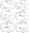 |
Fig. 5. Spectra obtained with the available observations (starting from GBM trigger time) from different instruments in six selected time bins on the basis of the presence of giga-electronvolt detections by Fermi/LAT and/or AGILE complemented with intrinsic spectra from LHAASO. Additional data from GBM (NaI4, NaI8, B1) and KONUS in these bins are shown, where available. Overall, the data show the existence of two separate components. The blue band, which spans energies from 10 keV to 100 GeV, represents the 65% confinement of the allowed flux around the best-fit model (marked with a solid blue line; see Table A.1). The green band, covering 10 MeV to 10 TeV, indicates the 65% confinement of the best-fit log-parabola model (best-fit model marked with a solid dark green line) for giga-electronvolt–tera-electronvolt energies. |
Deriving the “synthetic spectral data” based on the spectral parameters alone will lead to a loss of information because it will erase any evidence of the spectral curvature in the LHAASO band alone. However, after correcting for EBL absorption, the spectrum is compatible with a power law (see Figure 3 of The LHAASO Collaboration 2023) in the energy range 0.3–5 TeV: the loss of information is minimal. The evidence for curvature that we then find arises entirely from considering the tera-electronvolt data together with giga-electronvolt data.
3.3. Combined light curve in giga-electronvolt energies with AGILE and Fermi/LAT
LHAASO has identified a break around 600 s (from the GBM trigger time) in the light curve of GRB 221009A within the energy range of 0.3–5 TeV. The steepening of the VHE gamma-ray light curve observed by LHAASO is considered indicative of a jet break (Cao et al. 2023).
To investigate the cause of the slope change at 600 s post-GBM trigger, we generated a light curve for HE gamma rays using data from both Fermi/LAT and AGILE. We selected an energy range from 125 MeV to 3 GeV, which is covered by both instruments. This choice of 125 MeV adheres to the Fermi/LAT collaboration recommendation outlined in Bissaldi et al. (2023). Flux measurements in the 0.125–3 GeV range are presented in Table A.2. The data from AGILE that were initially in photon flux were converted to energy flux, as is detailed in Table A.3, assuming photon indices of −2.011. The conversion from the photon flux to the energy flux was performed using the equations mentioned below:
![Mathematical equation: $$ \begin{aligned} \mathrm F^{[E_1, E_2]}_{E} = F_{ph} \times log\left( \frac{E_2}{E_1}\right) \times \frac{E_1 E_2}{E_2-E_1}, \end{aligned} $$](/articles/aa/full_html/2025/09/aa54813-25/aa54813-25-eq6.gif) (2)
(2)
where F is the energy flux between the energy range of E1, E2. The energy flux in the band of [125 MeV, 3 GeV] was obtained with the following scaling factor:
![Mathematical equation: $$ \begin{aligned} \mathrm{F}^{ \mathrm 0.125-3\,GeV}_{\rm E} = \mathrm {log}\left(\frac{30}{0.125}\right) \times \frac{\mathrm{F^{E_1, E_2}_{E}}}{ \mathrm {log}(E_2/E_1) } = 5.48 \times \mathrm F^{[E_1, E_2]}_{ph} \times \frac{E_1 E_2}{E_2-E_1} .\end{aligned} $$](/articles/aa/full_html/2025/09/aa54813-25/aa54813-25-eq8.gif) (3)
(3)
The light curve is presented starting from a trigger time of 177 s, marking the detection of the initial gamma-ray pulse by KONUS (Frederiks et al. 2023).
Furthermore, we have incorporated low-energy data from Fermi/GBM in the 40 keV–40 MeV energy range (indicated by olive points in Figure 6). The kilo-electronvolt–mega-electronvolt emissions are classified into two time segments: the prompt phase (duration 100 s) and the combined prompt and afterglow phase (100–1000 s). It is observed that the combined prompt and afterglow emission phase post 600 s aligns with the temporal decline observed in the HE/VHE gamma rays.
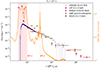 |
Fig. 6. Light curve of GRB 221009A observed with several instruments including LHAASO in the 0.3–5 TeV, Fermi/LAT and AGILE in the 0.1–3 GeV, and GBM and KONUS in the 0.04–40 MeV range. The two phases (BTI-1 and BTI-2) marked with a shaded red region denote the BTI intervals of Fermi/GBM. The orange line indicates the background-subtracted GBM light curve in counts/s. The magenta points are indicative of the KONUS flux in the prompt emission phase during BTI-1. The dark green data points are the flux points from GBM indicated as “prompt+afterglow” as during the period after BTI-1 the emission is a combination of prompt and afterglow. The details of the analysis of the Fermi/LAT data are discussed in Sect. 2. The AGILE data, obtained from Tavani et al. (2023), have been rescaled in the energy band 0.1–3 GeV. The light curve was plotted with the choice of a trigger time of T |


 |
Fig. 7. Variation in peak energy of the second spectral component (SSC component) as a function of time starting from 240 s after the trigger time of GBM until about 1500 s. No significant variation in the peak-energy has been observed mainly due to the larger uncertainty. The red band represents the 1-sigma confidence interval of the best-fit linear (pol-1) model. |
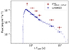 |
Fig. 8. Bolometric flux (between 10 MeV–10 TeV) of the second component estimated for selected time bins mentioned in Table 2. |
3.4. Extrapolation of prompt emission component in the giga-electronvolt band
Data from the temporal bins BIN-2, –6, –7, –8, –12, and –14 (see Fig. 5) were used to construct multiwavelength spectra in the range from kilo-electronvolts to tera-electronvolts. As is shown in Figure 6 and Table 2, depending on availability, the GBM and KONUS data were chosen covering the energy range of several tens of kilo-electronvolts to several tens of mega-electronvolts. Specifically for BIN-2, KONUS data were used, since GBM data were compromised by pile-up issues during this interval. For the remaining bins, we used the GBM data. Using the kilo-electronvolt–mega-electronvolt band data, we derived the optimal model parameters (see Table A.1). To assess the impact of the apparent initial peak within the giga-electronvolt–tera-electronvolt range, the spectrum was extended to 100 GeV. The extended models are represented by the shaded blue areas in Figure 5. The low-energy (sub-giga-electronvolt) spectral data from AGILE and Fermi/LAT overlap with the Band-function model extended up to 100 GeV (see Figure 6), meaning that the first hump influences the sub-giga-electronvolt emission. However, in bins such as BIN-2, –6, –7, –8, and –12, the observations above 1 GeV significantly surpass the extrapolated “first hump,” suggesting the presence of an additional spectral component at giga-electronvolt–tera-electronvolt energies. For BIN-14, spectral data ranging from 50 MeV to 1 GeV are adequately described by a single component that extends to several tens of giga-electronvolts. The upper limit set by AGILE at approximately 20 GeV is consistent with a second component, also constrained by the spectrum of LHAASO extending energies above 300 GeV.
4. Possible origin of giga-electronvolt–tera-electronvolt component
4.1. Synchrotron self-Compton model
To model the late-epoch (> 600 s) 40 keV–5 TeV spectrum of the afterglow radiation of GRB 221009A, we used the lepto-hadronic modeling code (LeHaMoC; Stathopoulos et al. 2024). Specifically, we adopted the leptonic module of LeHaMoC called LeMoC. We assumed that the spectra at the latest epochs are dominated by the synchrotron and inverse Compton radiation of power-law distributed electrons accelerated in the forward shock. LeMoC allowed us to estimate the energy losses of leptons (electrons and/or positrons) due to synchrotron radiation, inverse Compton scattering, synchrotron self-absorption, adiabatic losses, and photon-photon pair creation. The injection of particles was placed in a blob of radius Re, in a magnetic field of B. The following six free parameters were used to model the two-component kilo-electronvolt–tera-electronvolt spectrum of the afterglow: the strength of the magnetic field in the comoving frame, B, the minimum Lorentz factor of the injected electrons, γm, the maximum energy of the injected electrons, γmax, the shape of the injected electron spectrum, p (dN/dγ ∝ γe−p), the electron injection compactness, le = LeσT/4πRemec3 (Le is the injection luminosity of electrons), and the Doppler factor, D. We used the rough approximation for Re as  and Γ ≈ D/2, where
  s.
s.
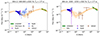 |
Fig. 9. Spectral energy distribution (SED) of GRB 221009A at the epochs with available LHAASO data: 600–800 s (BIN-12; top panel) and 1000–1350 s (BIN-14; bottom panel). Since these two SEDs are right after prompt emission, in the early afterglow phase, they are individually modeled in a SSC scenario. The shaded yellow area represents the 1σ confidence intervals of the best-fit model. Figures B.1 and B.2 display the posterior parameter distributions for these two epochs. Table 4 and Table 5 enlist the best-fit model parameters and their associated uncertainties, respectively. |
Best-fit parameters derived from the SSC model for the multiwavelength data of GRB 221009A at 600–800 s (BIN-12) and associated 1σ confidence interval.
Best-fit parameters derived from the SSC model for the multiwavelength data of GRB 221009A at 1000–1350 s (BIN-14) and associated 1σ confidence interval.
We used the emcee Python package (Foreman-Mackey et al. 2013) to sample the posterior probability density with the Markov chain Monte Carlo approach. Information on priors and posteriors is listed in Tables 4 and 5. The corner plots with the posterior distribution of six parameters are shown in Figures B.1 and B.2. We estimated the SSC spectra (Figure 10) and the light curve of the giga-electronvolt and tera-electronvolt emission (Figure 11) for earlier and the late epochs of observations by rescaling the SSC parameters. For the homogeneous medium, beyond the deceleration time, we expect  ,
,  ,
,  ,
,  ,
,  , and
, and  .
.
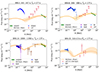 |
Fig. 10. Predicted SEDs for the early epochs: at 270–308 s (BIN-6) and 1000–1350 s (BIN-14). The SEDs were estimated from the posterior distribution of SSC model for the latest epoch at 600–800s (BIN-12), with the self-similar dynamics of the relativistic blast wave in the homogeneous (dark orange) circumburst medium. Note that these are not the fits to the data but predictions of the SEDs from the scaling of microphysical parameters according to the expected dynamics of the forward shock. |
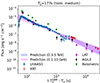 |
Fig. 11. Light curve of LHAASO (0.3–5 TeV; blue points) together with the expected light curve of the afterglow emission (light blue and purple band for tera-electronvolt and giga-electronvolt energies, respectively) in a homogeneous circumburst medium. The model was obtained using the median value of the microphysical parameters of the SSC model for the epoch at 600–800 s (BIN-12), with the self-similar dynamics of the relativistic blast wave. The bands are the predictions of the afterglow radiation at earlier and later epochs derived by the scaling of microphysical parameters according to the expected dynamics of the forward shock (see text for details). The green points represent the bolometric flux in the energy band 10 MeV–5 TeV derived from the analytical log-parabola modeling of the giga-electronvolt–tera-electronvolt hump (see Figure 8 for details). |
Regardless of the exact value of the density of the circumburst medium and the total kinetic energy of the jet, with LeMoC it is possible to estimate the broadband spectra of afterglow emission at other temporal epochs due to the self-similar nature of the relativistic blast-wave dynamics in the cold medium (Blandford & McKee 1976). To predict the expected kilo-electronvolt–tera-electronvolt afterglow emission at earlier or later epochs, we assumed that the equipartition parameters and the index of the accelerated electrons do not vary with time.
We also estimated the expected soft X-ray (0.5–5 keV) fluence in the afterglow phase for the first 20 minutes to be ∼6 × 10⁻⁴ erg cm−2, which is one order of magnitude less than what is required to explain the observed X-ray rings from GRB 221009A (Tiengo et al. 2023). The prompt emission in the brightest pulses has a flux of ∼6 × 10⁻⁶ erg cm−2 s−1 at 0.5–5 keV, once the Band function is extrapolated down to soft X-rays. Hundreds of seconds of prompt emission together with the early X-ray afterglow emission should be reasonable enough to account for the observed X-ray rings.
4.2. External injection of the prompt emission photons
During the first few hundred seconds, the mega-electronvolt prompt emission is luminous (up to ∼1056 erg/s). In the standard prompt emission model for internal shocks (Rees & Meszaros 1994), the mega-electronvolt radiation is far behind the forward shock. Thus, the supply of prompt emission photons to electrons accelerated in the forward shock and the photons produced by them cannot be ignored. There are several effects from the long-lasting (∼500 s) energy and photon supply: (1) additional energy injection into the decelerating blast wave (Derishev & Piran 2024), (2) γ − γ attenuation of tera-electronvolt photons (Khangulyan et al. 2024), and (3) suppression of electron cooling by mega-electronvolt photons and gain in photons from external inverse Compton (EIC) scattering of X-ray photons of the prompt emission.
There is a crucial difference between the two sources of the seed photons for the inverse Compton cooling of the forward shock-accelerated electrons and the subsequent pair production. The expected synchrotron photons from the forward shock electrons are softer, whereas the prompt are harder. Let us assume similar bulk Lorentz factors, Γ, for the mega-electronvolt region and the forward shock. The target photons for the pair production of observed 0.5 TeV would be  MeV photons of the prompt emission. The optical depth for pair production is then
  , where t is the observed time. Thus, the initial rise of the afterglow radiation could have been suppressed, which could explain the steep rise of the LHAASO light curve (Khangulyan et al. 2024; Gao & Zou 2024; Zhang et al. 2023a) (see also Shen et al. 2024). It can also slightly affect tera-electronvolt emission at later times, beyond the peak of the afterglow,
  (homogeneous medium).
On the one hand, the injection of prompt emission photons suppresses the tera-electronvolt afterglow radiation. On the other hand, the radiation from the EIC scattering of the prompt emission photons by the forward shock accelerated electrons provides an additional source of giga-electronvolt–tera-electronvolt photons to the standard SSC afterglow emission, but with a significant delay with respect to the mega-electronvolt injection time. The EIC radiation is anisotropic and most of the photons are received at an angle of ∼1/Γ with respect to the line of sight (Aharonian & Atoyan 1981; Brunetti 2000; Beloborodov 2005; Fan & Piran 2006; Fan et al. 2008; Zhang et al. 2021a,b). Therefore, the peak energy of EIC will also be further reduced. Consequently, the observed flux of the EIC will also be suppressed as a result of anisotropy. We expect the EIC radiation to have a duration of ∼R/cΓ2 ∼ 4t (homogenous circumburst medium) with respect to the observed time of prompt emission photons, where R is the size of the forward shock at a given observer time, t (Beloborodov 2005; Fan & Piran 2006). Therefore, the upscattered prompt emission photons lose their variability in the tera-electronvolt γ-rays. Effective EIC scattering is possible only with soft prompt emission photons with energy density, which scales as ∝Lγt1/2 (homogeneous circumburst medium).
At any time phase of the forward shock, the observed photons of the prompt emission of energy  are seen as
  MeV photons in the rest frame of the typical electrons accelerated by the forward shock. Therefore, only the prompt emission photons up to
  keV will contribute to the EIC radiation. At the coasting and deceleration time of the forward shock, the emitting region of the mega-electronvolt photons is expected to have a similar Γ as the forward shock; therefore, we can compare the X-ray flux of the prompt emission with the one expected from the afterglow radiation. The prompt emission provides ∼10 times more photons at ∼10 keV. However, the observed delayed EIC radiation is suppressed by a factor of ∼0.5 (Γ > 100), and the EIC would then provide only a slight addition to the observed giga-electronvolt photons. More importantly, because of the presence of mega-electronvolt photons of the prompt emission, the peak of the EIC radiation will be located at energies lower than the ones expected in the SSC model (fewer mega-electronvolt photons). In other words, the external field of mega-electronvolt photons softens the early tera-electronvolt spectra.
5. Discussion and conclusion
In the HE gamma rays from 50 MeV and up to 100 GeV, the Large Area Telescope (LAT) on board the Fermi satellite observed the burst from the onset until the GRB moved out of Fermi/LAT’s FoV around 400 s. Due to the high fluence in hard X-rays, the Fermi/LAT data experienced significant pile-up during the time interval 219–244 s and 255–270 s, making the giga-electronvolt data during these times unrecoverable. Data from 244–255 s and 270–280 s, while still affected by pile-up, could be analyzed using a specific method described in Bissaldi et al. (2023). AGILE recorded observations of GRB 221009A (Tavani et al. 2023). Specifically, it captured data during two separate intervals, 684.0–834.0 s and 1129.0–1279.0 s, which extend beyond the Fermi/LAT observation period (after 400 s) and closely align in timing (Tavani et al. 2023) with the intervals reported by LHAASO. Referring to time intervals prompted by LHAASO observations (see Table 2, spanning from BIN-0 to –14), we selected specific time bins based on the availability of quasi-simultaneous data from various instruments. The time bins and available data are shown in Figure 1. The bins of interest, specifically BIN-2: 242.0–247.0, BIN-3: 247.0–253.0, BIN-6: 270.0–308.0, BIN-7: 308.0–350.0, BIN-8: 350.0–401.0, BIN-12: 600.0–800.0, and BIN-14: 1000.0–1350.0, provide comprehensive data coverage from kilo-electronvolt to tera-electronvolt energies. The multiwavelength data for these bins are shown in Figure 5. Using these time bins, we constructed the multiwavelength spectrum (covering energies from kilo-electronvolts to tera-electronvolts) using the concurrent data available from kilo-electronvolt–mega-electronvolt (lower-energy band covered with Fermi/GBM and KONUS) to giga-electronvolt energies (Fermi/LAT and AGILE) along with the tera-electronvolt data from LHAASO. Observations from GBM and KONUS in mega-electronvolt energies were fit with a standard Band function for the prompt emission spectra (Band et al. 1993), with the exception of BIN-6, which in addition to a Band-function requires a distinct Gaussian line emission (the Ravasio line), as was discovered in Ravasio et al. (2024). The best-fit model parameters are stated in Table A.1. In each time bin, the model is then extended up to 100 GeV.
Across all the temporal bins mentioned above, the soft spectral slope of the emission at mega-electronvolt energies (see Table A.1, third column) and the presence of the giga-electronvolt–tera-electronvolt component exceeding the best-fit model from the kilo-electronvolt–mega-electronvolt band extended up to 100 GeV clearly indicate the emergence of a distinguished giga-electronvolt–tera-electronvolt spectral component. This is particularly evident in the earlier bins (such as BIN-2, BIN-6), where the source exhibits high-flux states across all energy bands. Moreover, (for example, BIN-2) a slope change in the giga-electronvolt data compared to the kilo-electronvolt–mega-electronvolt data has been observed, which further separates the giga-electronvolt–tera-electronvolt spectral component. For the final time bin, BIN-14, the Fermi/ GBM data extending up to 100 GeV (illustrated in the blue band in Figure 5) align with the flux and slope of the giga-electronvolt data obtained with AGILE. Consequently, the extended model, supported by observations by AGILE, predicts a flux in the VHE gamma rays that is a factor of 10 lower, as observed with LHAASO in the 0.3–5 TeV range, confirming the spectral turnover from mega-electronvolt to giga-electronvolt–tera-electronvolt components at late times beyond 1000 seconds.
We applied a log-parabola model to characterize the giga-electronvolt (observed with Fermi/LAT and AGILE) and tera-electronvolt (observed with LHAASO) data. For the six time intervals, we determined the peak position, peak flux, and bolometric flux in the energy band of 10 MeV to 10 TeV. We find that the peak position does not show significant variation and ranges between 10 GeV–300 GeV (see Figure 7). Instead, the peak positions estimated at later times (after 1000 s) are not well constrained due to the data quality in the giga-electronvolt band. The bolometric light curve in the energy band of 10 MeV–10 TeV roughly traces the light curve of LHAASO (see Figure 8).
To evaluate the underlying mechanism responsible for the broadband emission during the first 20 minutes, we constructed the light curve across the following energy bands: (1) 0.3–5 TeV (LHAASO), (2) 0.1–3 GeV (LAT and AGILE data when available) and (3) 0.04–40 MeV (GBM and KONUS). The multiwavelength light curve is shown in Figure 6. The choice of the 0.04–40 MeV energy band is because it is covered by both Fermi/GBM and KONUS, whereas 0.1–3 GeV is covered by both Fermi/LAT and AGILE. Furthermore, we considered a start time (T ) of 177 s, corresponding to the onset of the main mega-electronvolt burst following the precursor, observed with KONUS (Frederiks et al. 2023). We observe that the variability in the light curve becomes less pronounced starting from BIN-12, aligning with the period when the variable emission in GBM ceases, and shows a steady decline. This is indicative of the emergence of the afterglow emission.
The mega-electronvolt spectral component of GRB 221009A is dominated by the prompt emission for the first ∼500 s, as is inferred from its variability. Given the absence of variability in the tera-electronvolt light curve observed with LHAASO, the mega-electronvolt and giga-electronvolt–tera-electronvolt spectral components are not produced from the same emission region of the early epochs (< 500 s). In contrast, the late mega-electronvolt emission (> 600 s) is temporally featureless and can be assigned to the afterglow emission component, as has also been considered by other authors (Zhang et al. 2023b; Lesage et al. 2023; An et al. 2023; Zheng et al. 2024). We thus consider the latest (> 600 s) kilo-electronvolt–tera-electronvolt spectrum to arise from the synchrotron and synchrotron self-Compton (SSC) radiation of the forward shock-accelerated electrons of the circumburst medium. The 40 keV–1 MeV spectrum at the latest epoch (1000–1350 s) is best fit by the power-law model with the photon index of −2.14 ± 0.02. The 95% upper limit of the peak energy is 53 keV. The 100 MeV–5 TeV is described by a log-parabola model with a peak energy of ≈3 × 10⁵ MeV. In the SSC scenario, and assuming the Thomson regime, it would require electrons to have energies ≥0.3 GeV.
In this scenario, we access the microphysical parameters of the external shock modeling the joint kilo-electronvolt–tera-electronvolt spectrum of the afterglow emission at the latest epochs (600–800 s and 1000–1350 s) with the SSC model (see Figure 9). The data is best described by the soft electron population,  , where
  and
and  for the consecutive time bins. The inferred magnetic field in this one-zone model is
  G and
G and  G. We find that the energies of the injected electrons span at least three orders, reaching sub-tera-electronvolt energies (∼0.5 TeV). To reach an efficient acceleration in the relativistic shock, one would require a low magnetization of σ ≤ 3 × 10⁻⁵ in the electron-ion plasma (Sironi et al. 2013). To reach the inferred values of the magnetic field strength of B ∼ 0.1 G, it would be necessary to amplify the magnetic field in the downstream of the shock by a factor of
  with respect to the pre-shocked magnetic field, where n is the volume density of the circumburst medium.
Independent of the exact value of the density of the circumburst medium or the total kinetic energy of the jet, LeMoC enables the estimation of the broadband spectra of afterglow emissions at various time intervals due to the self-similar solution of the relativistic blast wave in a homogeneous medium (Blandford & McKee 1976). In order to forecast the expected kilo-electronvolt–tera-electronvolt afterglow emissions at earlier or later times, we assumed that the equipartition parameters and the index of the accelerated electrons remain unchanged over time. Under these assumptions, we derived the kilo-electronvolt–mega-electronvolt spectra of the SSC radiation of the afterglow at earlier and late epochs (see Figure 10). Additionally, to further test the model credibility, we introduced a time bin that extends beyond the LHAASO observation window; namely, BIN-15 (3.8–4.5 ks). During this time interval, the source was observed with Swift/BAT and Fermi/LAT. The proposed SSC afterglow model, when extrapolated to BIN-15, effectively accounts for the observed spectrum. We conclude that in the homogeneous circumburst case, the kilo-electronvolt–tera-electronvolt spectral data can be explained well by the predicted model. We also computed the expected giga-electronvolt–tera-electronvolt light curves in the SSC scenario (see Figure 11). The observed LHAASO light curve is in agreement with this simple model with slight deviations. However, one can notice that the observed tera-electronvolt spectra are slightly softer than expected. Figure 10 shows that the early giga-electronvolt emission is slightly above the SSC predictions. One possibility of interpreting these deviations is the external supply of prompt emission photons to electrons accelerated in the forward shock. The more accurate temporal evolution of the early giga-electronvolt–tera-electronvolt emission is not trivial to reproduce due to several complications, including the effects of preacceleration and the finite duration of the energy injection (Derishev & Piran 2024). However, here we focus on the extraction of the microphysical parameters from the exceptionally well-sampled kilo-electronvolt–tera-electronvolt observations of the afterglow radiation.
The broad energy coverage (40 keV–5 TeV) of the GRB 221009A prompt and afterglow spectra have allowed us to distinguish the low-energy kilo-electronvolt–mega-electronvolt synchrotron component and the spectral turnover to the second, VHE spectral component. In the six time-resolved spectra spanning the first 20 minutes after the GRB trigger, we found the VHE component to peak between 10–100 GeV. In later epochs (> 600 s), we obtained a two-component SED of the afterglow radiation. Assuming a leptonic origin of the afterglow radiation, we modeled the kilo-electronvolt–tera-electronvolt spectrum with the SSC model, assuming power-law distributed electrons in a single zone. The multiwavelength data are best described by a soft electron distribution: ( ). The strength of the magnetic field in the downstream of the shock is estimated to be on the order of ∼0.1 G. We used the results of modeling of single-epoch data to predict early kilo-electronvolt–tera-electronvolt data. In the simplest model assumptions of constant equipartition parameters and the expansion of the relativistic blast wave in the homogeneous medium, we obtained good agreement for the giga-electronvolt–tera-electronvolt light curve (Figure 11) and the SEDs (Figure 10).
The bin mentioned in Table 2 starts from 242.1 s, thus it covers a fraction of the entire bin of LHAASO.
LP is a preferred model for the HE-VHE spectral component in several VHE objects, such as the Crab Nebula (Aleksic et al. 2015); Mrk501 (Massaro et al. 2006); bright VHE blazars detected with HAWC (Jacobsen et al. 2023); and Fermi/LAT blazars with VHE emission (Zhou et al. 2021).
This assumption of a photon index of −2.0 is consistent with Tavani et al. (2023) to analyze GRID observations in the energy range of 50 MeV to 3 GeV as described in Section B.1.
Acknowledgments
The authors thank Lara Nava, Om Sharan Salafia, Maria Edvige Ravasio, Luca Foffano, Annalisa Celotti, Giancarlo Ghirlanda, Elena Amato and Ulyana Dupletsa for the fruitful discussions. We acknowledge the CINECA award under the ISCRA initiative, for the availability of high-performance computing resources and support. We acknowledge the ModIC 2024 workshop (https://indico.gssi.it/event/606/) for providing an interdisciplinary platform for fruitful discussion. BB expresses gratitude to Dr. Francesco Viola for supporting the access of the GSSI computing resources. The authors thank the Director and the Computing and Network Service of the Laboratori Nazionali del Gran Sasso (LNGS-INFN). This research used resources of the LNGS HPC cluster realized in the framework of Spoke 0 and Spoke 5 of the ICSC project – Centro Nazionale di Ricerca in High Performance Computing, Big Data and Quantum Computing, funded by the NextGenerationEU European initiative through the Italian Ministry of University and Research, PNRR Mission 4, Component 2: Investment 1.4, Project code CN00000013 – CUP I53C21000340006. BB and MB acknowledge financial support from the Italian Ministry of University and Research (MUR) for the PRIN grant METE under contract no. 2020KB33TP. The work of DDF, AAL, DSS, and AET is supported by the basic funding program of the Ioffe Institute FFUG-2024-0002. AET also acknowledges accordo ASI e INAF HERMES 2022-25-HH.0.
References
- Abdalla, H., Adam, R., Aharonian, F., et al. 2019, Nature, 575, 464 [Google Scholar]
- Abdalla, H., Aharonian, F., Ait Benkhali, F., et al. 2021, Science, 372, 1081 [NASA ADS] [CrossRef] [Google Scholar]
- Abe, H., Abe, S., Acciari, V. A., et al. 2023, MNRAS, 527, 5856 [Google Scholar]
- Aharonian, F. A., & Atoyan, A. M. 1981, Astrophys. Space Sci., 79, 321 [Google Scholar]
- Ajello, M., Arimoto, M., Axelsson, M., et al. 2019, ApJ, 878, 52 [NASA ADS] [CrossRef] [Google Scholar]
- Ajello, M., Arimoto, M., Axelsson, M., et al. 2020, ApJ, 890, 9 [Google Scholar]
- Aleksic, J., Ansoldi, S., Antonelli, L., et al. 2015, J. High Energy Astrophys., 5, 30 [Google Scholar]
- An, Z. H., Antier, S., Bi, X. Z., et al. 2023, ArXiv e-prints [arXiv:2303.01203] [Google Scholar]
- Band, D., Matteson, J., Ford, L., et al. 1993, ApJ, 413, 281 [Google Scholar]
- Beloborodov, A. M. 2005, ApJ, 618, L13 [Google Scholar]
- Biltzinger, B., Kunzweiler, F., Greiner, J., Toelge, K., & Burgess, J. M. 2020, A&A, 640, A8 [NASA ADS] [CrossRef] [EDP Sciences] [Google Scholar]
- Bissaldi, E., Bruel, P., Omodei, N., Pillera, R., & Di Lalla, N. 2023, Proc. Sci., ICRC2023, 847 [Google Scholar]
- Blandford, R. D., & McKee, C. F. 1976, Phys. Fluids, 19, 1130 [Google Scholar]
- Bright, J. S., Rhodes, L., Farah, W., et al. 2023, Nat. Astron., 7, 986 [NASA ADS] [CrossRef] [Google Scholar]
- Brunetti, G. 2000, Astropart. Phys., 13, 107 [Google Scholar]
- Buchner, J. 2016, Astrophysics Source Code Library [record ascl:1610.011] [Google Scholar]
- Burns, E., Svinkin, D., Fenimore, E., et al. 2023, ApJ, 946, L31 [NASA ADS] [CrossRef] [Google Scholar]
- Cao, Z., Aharonian, F., An, Q., et al. 2023, Science, 380, 1390 [NASA ADS] [CrossRef] [Google Scholar]
- Cao, Z., Aharonian, F., An, Q., et al. 2024, ApJS, 271, 25 [NASA ADS] [CrossRef] [Google Scholar]
- Derishev, E., & Piran, T. 2024, MNRAS, 530, 347 [NASA ADS] [CrossRef] [Google Scholar]
- De Santis, A. 2024, https://github.com/LudovicoAlt/py3 [Google Scholar]
- Fan, Y., & Piran, T. 2006, MNRAS, 370, L24 [Google Scholar]
- Fan, Y.-Z., Piran, T., Narayan, R., & Wei, D.-M. 2008, MNRAS, 384, 1483 [Google Scholar]
- Fermi LAT Team 2022, GRB Coordinates Network, 32658, 1 [NASA ADS] [Google Scholar]
- Fitzpatrick, G., Connaughton, V., McBreen, S., & Tierney, D. 2011, arXiv e-prints [arXiv:1111.3779] [Google Scholar]
- Foreman-Mackey, D., Hogg, D. W., Lang, D., & Goodman, J. 2013, PASP, 125, 306 [Google Scholar]
- Fraija, N., Dainotti, M. G., Betancourt Kamenetskaia, B., Galván-Gámez, A., & Aguilar-Ruiz, E. 2024, MNRAS, 527, 1884 [Google Scholar]
- Frederiks, D., Svinkin, D., Lysenko, A. L., et al. 2023, ApJ, 949, L7 [NASA ADS] [CrossRef] [Google Scholar]
- Gao, D.-Y., & Zou, Y.-C. 2024, ApJ, 961, L6 [NASA ADS] [CrossRef] [Google Scholar]
- Giarratana, S., et al. 2024, A&A, 690, A74 [NASA ADS] [CrossRef] [EDP Sciences] [Google Scholar]
- Jacobsen, S., Linden, T., & Freese, K. 2023, JCAP, 2023, 009 [CrossRef] [Google Scholar]
- Khangulyan, D., Aharonian, F., & Taylor, A. M. 2024, ApJ, 966, 31 [Google Scholar]
- Laskar, T., Alexander, K. D., Margutti, R., et al. 2023, ApJ, 946, L23 [NASA ADS] [CrossRef] [Google Scholar]
- Lesage, S., Veres, P., Briggs, M. S., et al. 2023, ApJ, 952, L42 [NASA ADS] [CrossRef] [Google Scholar]
- MAGIC Collaboration (Acciari, V. A., et al.) 2019, Nature, 575, 455 [Google Scholar]
- Malesani, D. B., Levan, A. J., Izzo, L., et al. 2025, A&A, in press, https://doi.org/10.1051/0004-6361/202346146 [Google Scholar]
- Massaro, E., Tramacere, A., Perri, M., Giommi, P., & Tosti, G. 2006, A&A, 448, 861 [NASA ADS] [CrossRef] [EDP Sciences] [Google Scholar]
- Mészáros, P., & Rees, M. J. 1997, ApJ, 476, 232 [CrossRef] [Google Scholar]
- Miceli, D., & Nava, L. 2022, Galaxies, 10, 66 [NASA ADS] [CrossRef] [Google Scholar]
- Nava, L. 2018, Int. J. Mod. Phys. D, 27, 1842003 [NASA ADS] [CrossRef] [Google Scholar]
- Nava, L. 2021, Universe, 7, 503 [NASA ADS] [CrossRef] [Google Scholar]
- O’Connor, B., Troja, E., Ryan, G., et al. 2023, Sci. Adv., 9, eadi1405 [CrossRef] [Google Scholar]
- Paczynski, B., & Rhoads, J. E. 1993, ApJ, 418, L5 [NASA ADS] [CrossRef] [Google Scholar]
- Ravasio, M. E., Salafia, O. S., Oganesyan, G., et al. 2024, Science, 385, 452 [Google Scholar]
- Rees, M. J., & Meszaros, P. 1994, ApJ, 430, L93 [Google Scholar]
- Ren, J., Wang, Y., & Dai, Z.-G. 2024, ApJ, 962, 115 [NASA ADS] [CrossRef] [Google Scholar]
- Salafia, O. S., Ravasio, M. E., Yang, J., et al. 2022, ApJ, 931, L19 [NASA ADS] [CrossRef] [Google Scholar]
- Sari, R., & Esin, A. A. 2001, ApJ, 548, 787 [NASA ADS] [CrossRef] [Google Scholar]
- Sari, R., Piran, T., & Narayan, R. 1998, ApJ, 497, L17 [Google Scholar]
- Sato, Y., Murase, K., Ohira, Y., & Yamazaki, R. 2023, MNRAS, 522, L56 [NASA ADS] [CrossRef] [Google Scholar]
- Shen, J.-Y., Zou, Y.-C., Chen, A. M., & Gao, D.-Y. 2024, MNRAS, 529, L19 [Google Scholar]
- Sironi, L., Spitkovsky, A., & Arons, J. 2013, ApJ, 771, 54 [Google Scholar]
- Stathopoulos, S. I., Petropoulou, M., Vasilopoulos, G., & Mastichiadis, A. 2024, A&A, 683, A225 [NASA ADS] [CrossRef] [EDP Sciences] [Google Scholar]
- Tavani, M., Piano, G., Bulgarelli, A., et al. 2023, ApJ, 956, L23 [Google Scholar]
- The LHAASO Collaboration 2023, Sci. Adv., 9, eadj2778 [CrossRef] [Google Scholar]
- Tiengo, A., Pintore, F., Vaia, B., et al. 2023, ApJ, 946, L30 [NASA ADS] [CrossRef] [Google Scholar]
- Veres, P., Bhat, P. N., Briggs, M. S., et al. 2019, Nature, 575, 459 [NASA ADS] [CrossRef] [Google Scholar]
- Wang, K., Tang, Q. W., Zhang, Y. Q., et al. 2023, ArXiv e-prints [arXiv:2310.11821] [Google Scholar]
- Zhang, B. T., Murase, K., Yuan, C., Kimura, S. S., & Mészáros, P. 2021a, ApJ, 908, L36 [NASA ADS] [CrossRef] [Google Scholar]
- Zhang, B. T., Murase, K., Veres, P., & Mészáros, P. 2021b, ApJ, 920, 55 [Google Scholar]
- Zhang, B. T., Murase, K., Ioka, K., et al. 2023a, ApJ, 947, L14 [NASA ADS] [CrossRef] [Google Scholar]
- Zhang, H.-M., Huang, Y.-Y., Liu, R.-Y., & Wang, X.-Y. 2023b, ApJ, 956, L21 [CrossRef] [Google Scholar]
- Zheng, C., Zhang, Y.-Q., Xiong, S.-L., et al. 2024, ApJ, 962, L2 [Google Scholar]
- Zhou, R. X., Zheng, Y. G., Zhu, K. R., & Kang, S. J. 2021, ApJ, 915, 59 [NASA ADS] [CrossRef] [Google Scholar]
Appendix A: Data analysis summary
The data analysis results of GBM, LAT and AGILE are reported in Tables A.1, A.2, and A.3, respectively.
The parameters of the spectral model of GRB 221009A observed with Fermi/GBM for bins which are relevant for the multiwavelength analysis.
The observed flux in the 0.1-3 GeV energy band observed with Fermi/LAT.
The energy flux of AGILE. The photon flux as observed with AGILE has been converted to the energy flux as prescribed in Eq. 2 and 3.
Appendix B: Posteriror distribution of the model parameters:
The posterior distribution (corner plots) of the model parameters are stated in Figures B.1 and B.2. See Sect. 4 for details of the modeling.
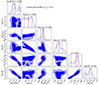 |
Fig. B.1. Corner plot showing the one- and two-sigma contours of the joint two-dimensional posteriors for each parameter pair for SSC model of the kilo-electronvolt–tera-electronvolt spectrum at 600-800 s (BIN-12). |
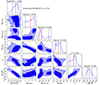 |
Fig. B.2. Corner plot showing the one- and two-sigma contours of the joint two-dimensional posteriors for each parameter pair for SSC model of the kilo-electronvolt–tera-electronvolt spectrum at 1000-1350 s (BIN-14). |
All Tables
Best-fit parameters derived from the SSC model for the multiwavelength data of GRB 221009A at 600–800 s (BIN-12) and associated 1σ confidence interval.
Best-fit parameters derived from the SSC model for the multiwavelength data of GRB 221009A at 1000–1350 s (BIN-14) and associated 1σ confidence interval.
The parameters of the spectral model of GRB 221009A observed with Fermi/GBM for bins which are relevant for the multiwavelength analysis.
The energy flux of AGILE. The photon flux as observed with AGILE has been converted to the energy flux as prescribed in Eq. 2 and 3.
All Figures
|
Fig. 1. Illustration of the data availability in each time bin (time stamps indicated in the vertical axis on the left and numbered bins on the right) for each instrument (see Table 2). Areas marked with slashes indicate bins impacted by pile-up in both Fermi/GBM and Fermi/LAT. A simple double-hump spectrum is shown to indicate the preliminary peak positions of the two components seen in GRB 221009A. The selection of time bins is based on the presence of multiwavelength data spanning kilo-electronvolt to tera-electronvolt energies. Six bins (BIN-2, −6, −7, −8, −12, and −14) were chosen for time-resolved spectral analysis. |
| In the text | |
|
Fig. 2. Energy flux observed with LHAASO extracted from publicly available data (Cao et al. 2023) for the periods reported with spectral index. In the analyzed time segments (named time bins: see Table 2) the light curve of LHAASO has been fit with a constant (pol-0) that represents the flux of GRB 221009A for that period. The blue markers in the top panel report the rebinned LHAASO flux for each period. The bottom panel reports the intrinsic spectral index observed with only LHAASO. |
| In the text | |
|
Fig. 3. Comparison of the backgrounds above 1 MeV estimated with the OSV tool and the polynomial fit for GRB 221009A. The top panel represents the light curve above 1 MeV. The OSV background uses Poisson uncertainty for each bin, which is omitted graphically for visual clarity. |
| In the text | |
|
Fig. 4. Light curve of GRB 221009A above 1 MeV with polynomial fit considering alternative methods. |
| In the text | |
|
Fig. 5. Spectra obtained with the available observations (starting from GBM trigger time) from different instruments in six selected time bins on the basis of the presence of giga-electronvolt detections by Fermi/LAT and/or AGILE complemented with intrinsic spectra from LHAASO. Additional data from GBM (NaI4, NaI8, B1) and KONUS in these bins are shown, where available. Overall, the data show the existence of two separate components. The blue band, which spans energies from 10 keV to 100 GeV, represents the 65% confinement of the allowed flux around the best-fit model (marked with a solid blue line; see Table A.1). The green band, covering 10 MeV to 10 TeV, indicates the 65% confinement of the best-fit log-parabola model (best-fit model marked with a solid dark green line) for giga-electronvolt–tera-electronvolt energies. |
| In the text | |
|
Fig. 6. Light curve of GRB 221009A observed with several instruments including LHAASO in the 0.3–5 TeV, Fermi/LAT and AGILE in the 0.1–3 GeV, and GBM and KONUS in the 0.04–40 MeV range. The two phases (BTI-1 and BTI-2) marked with a shaded red region denote the BTI intervals of Fermi/GBM. The orange line indicates the background-subtracted GBM light curve in counts/s. The magenta points are indicative of the KONUS flux in the prompt emission phase during BTI-1. The dark green data points are the flux points from GBM indicated as “prompt+afterglow” as during the period after BTI-1 the emission is a combination of prompt and afterglow. The details of the analysis of the Fermi/LAT data are discussed in Sect. 2. The AGILE data, obtained from Tavani et al. (2023), have been rescaled in the energy band 0.1–3 GeV. The light curve was plotted with the choice of a trigger time of T |
| In the text | |
|
Fig. 7. Variation in peak energy of the second spectral component (SSC component) as a function of time starting from 240 s after the trigger time of GBM until about 1500 s. No significant variation in the peak-energy has been observed mainly due to the larger uncertainty. The red band represents the 1-sigma confidence interval of the best-fit linear (pol-1) model. |
| In the text | |
|
Fig. 8. Bolometric flux (between 10 MeV–10 TeV) of the second component estimated for selected time bins mentioned in Table 2. |
| In the text | |
|
Fig. 9. Spectral energy distribution (SED) of GRB 221009A at the epochs with available LHAASO data: 600–800 s (BIN-12; top panel) and 1000–1350 s (BIN-14; bottom panel). Since these two SEDs are right after prompt emission, in the early afterglow phase, they are individually modeled in a SSC scenario. The shaded yellow area represents the 1σ confidence intervals of the best-fit model. Figures B.1 and B.2 display the posterior parameter distributions for these two epochs. Table 4 and Table 5 enlist the best-fit model parameters and their associated uncertainties, respectively. |
| In the text | |
|
Fig. 10. Predicted SEDs for the early epochs: at 270–308 s (BIN-6) and 1000–1350 s (BIN-14). The SEDs were estimated from the posterior distribution of SSC model for the latest epoch at 600–800s (BIN-12), with the self-similar dynamics of the relativistic blast wave in the homogeneous (dark orange) circumburst medium. Note that these are not the fits to the data but predictions of the SEDs from the scaling of microphysical parameters according to the expected dynamics of the forward shock. |
| In the text | |
|
Fig. 11. Light curve of LHAASO (0.3–5 TeV; blue points) together with the expected light curve of the afterglow emission (light blue and purple band for tera-electronvolt and giga-electronvolt energies, respectively) in a homogeneous circumburst medium. The model was obtained using the median value of the microphysical parameters of the SSC model for the epoch at 600–800 s (BIN-12), with the self-similar dynamics of the relativistic blast wave. The bands are the predictions of the afterglow radiation at earlier and later epochs derived by the scaling of microphysical parameters according to the expected dynamics of the forward shock (see text for details). The green points represent the bolometric flux in the energy band 10 MeV–5 TeV derived from the analytical log-parabola modeling of the giga-electronvolt–tera-electronvolt hump (see Figure 8 for details). |
| In the text | |
|
Fig. B.1. Corner plot showing the one- and two-sigma contours of the joint two-dimensional posteriors for each parameter pair for SSC model of the kilo-electronvolt–tera-electronvolt spectrum at 600-800 s (BIN-12). |
| In the text | |
|
Fig. B.2. Corner plot showing the one- and two-sigma contours of the joint two-dimensional posteriors for each parameter pair for SSC model of the kilo-electronvolt–tera-electronvolt spectrum at 1000-1350 s (BIN-14). |
| In the text | |
Current usage metrics show cumulative count of Article Views (full-text article views including HTML views, PDF and ePub downloads, according to the available data) and Abstracts Views on Vision4Press platform.
Data correspond to usage on the plateform after 2015. The current usage metrics is available 48-96 hours after online publication and is updated daily on week days.
Initial download of the metrics may take a while.