| Issue |
A&A
Volume 701, September 2025
|
|
|---|---|---|
| Article Number | A38 | |
| Number of page(s) | 15 | |
| Section | Extragalactic astronomy | |
| DOI | https://doi.org/10.1051/0004-6361/202555205 | |
| Published online | 04 September 2025 | |
Galaxies at the edges: A complete census of the MACS J0416.1–2403 cluster
1
INAF – Osservatorio Astronomico di Capodimonte, Salita Moiariello 16, 80131 Napoli, Italy
2
Università di Salerno, Dipartimento di Fisica “E.R. Caianiello”, Via Giovanni Paolo II 132, 84084 Fisciano (SA), Italy
3
Dipartimento di Fisica e Scienze della Terra, Università degli Studi di Ferrara, Via Saragat 1, 44122 Ferrara, Italy
4
INFN – Gruppo Collegato di Salerno – Sezione di Napoli, Dipartimento di Fisica “E.R. Caianiello”, Università di Salerno, Via Giovanni Paolo II, 132, 84084 Fisciano (SA), Italy
5
INAF – Osservatorio Astronomico di Brera, Via Brera 28, I-20121 Milano, Italy
6
Dipartimento di Fisica dell’Università degli Studi di Trieste – Sezione di Astronomia, Via Tiepolo 11, I-34143 Trieste, Italy
7
INAF – Osservatorio Astronomico di Trieste, Via Tiepolo 11, I-34143 Trieste, Italy
8
Centro de Astrobiología (CAB), CSIC-INTA, Ctra. de Ajalvir km 4, Torrejón de Ardoz, 28850 Madrid, Spain
9
Thales Alenia Space, Via E. Mattei 1, 20064 Gorgonzola, Italy
10
Dipartimento di Fisica, Università degli Studi di Milano, Via Celoria 16, I-20133 Milano, Italy
11
INAF – IASF Milano, Via A. Corti 12, I-20133 Milano, Italy
12
INAF – Osservatorio Astronomico di Padova, Vicolo dell’Osservatorio 5, I-35122 Padova, Italy
13
Dipartimento di Fisica e Astronomia “G. Galilei”, Università di Padova, Via Marzolo 8, 35131 Padova, Italy
14
INAF – OAS, Osservatorio di Astrofisica e Scienza dello Spazio di Bologna, Via Gobetti 93/3, I-40129 Bologna, Italy
15
Max-Planck-Institut für Physik, Boltzmannstr. 8, 85748 Garching, Germany
16
Universitäts-Sternwarte München, Fakultät für Physik, Ludwig-Maximilians-Universität München, Scheinerstr. 1, 81679 München, Germany
17
Max-Planck-Institut für Extraterrestrische Physik, Giessenbachstr. 1, 85748 Garching, Germany
18
Department of Physics “E. Pancini”, University Federico II, Via Cintia 21, 80126 Napoli, Italy
19
TUM School of Natural Sciences, Technical University of Munich, Garching 85748, Germany
20
Dipartimento di Fisica e Geologia, Università degli Studi di Perugia, Via Alessandro Pascoli, s.n.c., 06123 Perugia, Italy
21
INFN Sezione di Perugia, Via Alessandro Pascoli, s.n.c., 06123 Perugia, Italy
⋆ Corresponding author: This email address is being protected from spambots. You need JavaScript enabled to view it.
Received:
18
April
2025
Accepted:
19
June
2025
Abstract
Context. Numerous studies have established that the physical properties of a galaxy are profoundly influenced by its surrounding environment. While gas inflows can supply the necessary fuel for star formation, high-density and high-temperature conditions can suppress star-forming activity through various quenching processes. Investigations into large-scale structures, such as filaments and overdense regions in the cluster outskirts at R ≥ 2R200, have predominantly focused on the low-z Universe. To move to intermediate-z and explore galaxy pathways combined with environmental effects, it is crucial to join wide-field spectroscopy and deep photometry.
Aims. Our primary objective is to spectroscopically analyse the photometric overdensity structures previously observed in the outskirts of the massive cluster MACS J0416.1−2403 (z = 0.397), interpreted as evidence of ongoing group infall into the cluster. With this study we aim to enhance our understanding of the evolutionary processes occurring within these substructures and their role in the pre-processing scenario. Additionally, we aim to investigate the global behaviour of galaxies in the outskirts in relation to their g − r colour, K-band luminosity (a proxy for stellar mass), and local density, emphasizing the influence of the environment on galaxy evolution.
Methods. We conducted a spectroscopic analysis extending to the outskirts up to 5.5R200 (∼10 Mpc), using the AAOmega spectrograph. The large field of view (1 deg2) and depth of the observations allowed us to explore galaxies up to the cluster’s periphery and across a wide stellar mass range, reaching down to the limit of dwarf galaxies. Redshifts were obtained through independent but comparable methods: Redrock, EZ, and Redmost, ensuring consistency and accuracy in our measurements.
Results. We identified 148 new spectroscopic cluster members from a sample of 1236 objects. We found that 81 out of the 148 galaxies are located in filamentary and overdense regions, supporting the role of filamentary infall in the cluster mass assembly history. A spectral analysis revealed that galaxies in high-density regions are more massive, redder, and more passive, compared to galaxies in low-density regions that appear to be bluer, less massive, and more star-forming. These findings underscore the significance of environmental effects, particularly in overdense regions, and the role of pre-processing phenomena in shaping galaxy properties before cluster infall.
Key words: catalogs / galaxies: clusters: general / galaxies: clusters: intracluster medium / galaxies: distances and redshifts / galaxies: evolution / galaxies: general
© The Authors 2025
 Open Access article, published by EDP Sciences, under the terms of the Creative Commons Attribution License (https://creativecommons.org/licenses/by/4.0), which permits unrestricted use, distribution, and reproduction in any medium, provided the original work is properly cited.
This article is published in open access under the Subscribe to Open model. This email address is being protected from spambots. You need JavaScript enabled to view it. to support open access publication.
1. Introduction
In the most widely accepted cosmological model, the Λ-Cold Dark Matter (ΛCDM) scenario, the formation and evolution of the structures occur hierarchically. In this framework, galaxy clusters, which are the largest gravitationally bound structures known in the Universe, are expected to grow and evolve over time via sequential mergers and accretion of material from the surrounding structures in their outer regions (e.g. Kauffmann et al. 1999a,b; De Lucia et al. 2006). The evolution of these rich and extended structures proceeds by assembling galaxy groups and individual galaxies. Galaxies accreted at the outskirts of clusters encounter the intracluster medium (ICM) and interact with this dense environment. Thus, galaxy clusters are ideal laboratories for studying the impact of accretion through the outer regions on galaxy evolution. One of the key unresolved questions in galaxy evolution is understanding how, when, and where galaxy properties transform. The population of infall galaxies that interact with the hot ionized gas of the ICM are subjected to external processes that involve a large variety of mechanisms, including ram pressure stripping (e.g. Gunn & Gott 1972), strangulation (e.g. Larson et al. 1980; Balogh et al. 2000), galaxy-galaxy interactions (e.g. Mihos & Hernquist 1996; Moore et al. 1998), tidal stripping (e.g. Zwicky 1951; Gnedin 2003; Villalobos et al. 2014), and thermal evaporation (e.g. Cowie & Songaila 1977). Any removal or consumption of gas typically results in a reduction or inhibition of star formation, leading to galaxy quenching. Consequently, cluster galaxies exhibit different properties compared to field galaxies, although field galaxies can also be quenched (e.g. Dressler 1980; Poggianti et al. 1999). Since the properties of the ICM change from the cluster core to the outskirts (Nagai & Lau 2011; Ichikawa et al. 2013; Lau et al. 2015; Biffi et al. 2018; Mirakhor & Walker 2021), the efficiencies of all these processes are inhomogeneous in the intracluster space, and the galaxies in the outer regions are expected to interact differently with the ICM, showing different properties. Moreover, in the outskirts of clusters, structures resembling galaxy groups that have already transformed due to dense environments can be observed before they experience infall into the cluster as a group, a phenomenon known as pre-processing (e.g. Zabludoff & Mulchaey 1998; Mulchaey & Zabludoff 1998; Mihos 2004; Fujita 2004; Ragusa et al. 2021, 2022, 2023). Massive galaxy clusters, such as the target of this work, MACS J0416.1−2403 (hereafter MACS0416), provide an exceptional environment for studying these processes, due to their rich and diverse galaxy populations. It offers a unique opportunity to study environmental effects and the collisional behaviour of both luminous and dark matter during cluster formation. Previous studies of galaxy populations infalling into clusters have largely focused on low-redshift systems (Paccagnella et al. 2016, 2017, 2019; Salerno et al. 2020), and it is crucial to extend these observations to higher redshifts. Despite the significant advancements in our understanding, there remains an ongoing debate about the exact evolutionary trajectories of galaxies and the importance of different quenching mechanisms of both mass-related processes (e.g. feedback from active galactic nuclei or supernovae) and environmental factors (e.g. ram pressure stripping, tidal forces, harassment, collisions between galaxy groups and clusters, and gas depletion). These mechanisms likely vary in impact, depending on the redshift and environment in which they occur (e.g. Annunziatella et al. 2016). To fully tackle this issue, it is crucial to observe galaxy populations across a wide range of environments, from those falling into the cluster to those in more isolated regions. This includes a diversity of halo masses and captures snapshots of galaxy evolution during periods of rapid transformation. Such a comprehensive approach will provide deeper insight into the interplay between the internal and external forces driving galaxy evolution at various stages. Despite the wealth of data on the central regions of galaxy clusters, our understanding of the physical processes taking place in the outermost regions, up to several virial radii, remains incomplete. The accretion through the outskirts is still an underexplored domain (Dekel et al. 2009; Danovich et al. 2012; Walker et al. 2019; Welker et al. 2020). This is partly due to the observational challenges in probing the lower-density outer regions of galaxy clusters, where the ICM is less dense, and thus harder to detect in X-ray and Sunyaev–Zeldovich observations. Furthermore, most studies focus on the central regions, covering only a fraction of the ICM volume. At the same time, the outskirts can reveal critical information about gas accretion, dark matter distribution, and galaxy transformation mechanisms beyond the dense cluster core. At intermediate redshifts (z ∼ 0.4), the lack of comprehensive observational campaigns targeting the cluster outskirts beyond 2−3 virial radii leaves a significant gap in our understanding of mass assembly processes. Observing galaxies out to 5R200 is crucial, as this is where galaxies undergo pre-processing in group environments before falling into the cluster (Fujita 2004). The outer regions also offer key insights into dark matter dynamics, including the role of caustics in the dark matter density profile (Mansfield et al. 2017; Diemer et al. 2017) and the contribution of turbulent gas motions (Lau et al. 2009; Vazza et al. 2009; Battaglia et al. 2012). Furthermore, characterizing the gas dynamics in these regions can shed light on non-equilibrium processes affecting the ICM, such as bulk and turbulent gas flows (Rudd & Nagai 2009) and an inhomogeneous gas density distribution (Nagai & Lau 2011; Roncarelli et al. 2013). With this work we aim to expand the existing Multi Unit Spectroscopic Explorer (MUSE) and VIsible Multi-Object Spectrograph (VIMOS) data (CLASH-VLT; Rosati et al. 2014) by targeting, with the 2dF+AAOmega instrument, a larger region of MACSJ0416 up to 5.5R200 (R200 = 1.82 Mpc), building on the low- and medium-resolution data previously collected for ∼4700 galaxies, of which ∼950 are confirmed cluster members. Complementary to these data, further observations from the cluster’s core, such as the Grism Lens-Amplified Survey from Space (GLASS; Treu et al. 2015; Vulcani et al. 2016, 2017) spectroscopic data, and archival MUSE integral-field spectrometry (Caminha et al. 2017), will enhance the study’s depth. This campaign will integrate multi-wavelength observations, including optical data from VLT Survey Telescope (VST) (Estrada et al. 2023), near-infrared (NIR) data from Visible and Infrared Survey Telescope for Astronomy (VISTA), X-ray, and radio datasets, to provide a well-rounded view of galaxy populations within the cluster up to the periphery. The comprehensive dataset will include galaxies down to the dwarf regime (stellar mass ∼109 M⊙), allowing a complete exploration of galaxy evolution from the cluster core to well beyond the virial radius.
The paper is organized as follows. In Sect. 2 we describe the state of the art with regard to MACS0416 at the time of this work. We illustrate the observations, the data reduction, and the data analysis in terms of redshift measurements in Sect. 3. In Sect. 4 we report the AAOmega spectroscopic catalogue and the criteria for the member selection. In Sect. 5 we present the results: in Sects. 5.1, 5.2, and 5.3 we qualitatively analyse the spectral properties of the galaxies in our sample of members with respect to the g − r colour, the magnitude in the K-band as a proxy of the stellar mass, and the properties of the galaxies within the different density ranges in the field of view (FoV), respectively. Finally, in Sect. 6 we summarize our results and conclusions.
Throughout the paper, we adopt the ΛCDM cosmology with Ωm = 0.3, ΩΛ = 0.7, and H0 = 70 km s−1 Mpc−1. Therefore, 1 arcmin corresponds to ∼0.321 Mpc at z = 0.397. All magnitudes are given in the AB system.
2. MACS J0416.1–2403
MACS0416 is a massive galaxy cluster located at redshift z = 0.397 ± 0.001 (∼4.26 Gyr, i.e. 30% of the lookback time to the Big Bang, Balestra et al. 2016), particularly known for its strong lensing effects and its complex structure. Figure 1 shows images of MACS0416 obtained using all the photometric data available at the time this work was written. Galaxies for which spectroscopic redshifts were obtained with MUSE (in red) or VIMOS (in blue) are marked in the top left panel. The colour composite image of the HST FoV is illustrated in the bottom left panel, while that from the VST g- and i-bands plus the VISTA Ks-band is shown in the right panel. The cluster, originally identified as part of the MACS survey (Ebeling et al. 2001), is characterized by high X-ray luminosity LX (L500) = (1.62 ± 0.02)×1045 L⊙ (Ogrean et al. 2016) and by a very high total mass of approximately M200 = 1.04 × 10¹⁵ M⊙ (Umetsu et al. 2014). Mann & Ebeling (2012) classified MACS0416 as a merger system, due to its irregular X-ray morphology and the projected separation of roughly 200 kpc between the two brightest cluster galaxies (BCGs). In support of this, the weak and strong lensing analyses (Zitrin et al. 2013; Jauzac et al. 2014, 2015; Grillo et al. 2015; Richard et al. 2014; Hoag et al. 2016; Caminha et al. 2017; Bonamigo et al. 2017, 2018; Chirivì et al. 2018; Bergamini et al. 2023) have revealed an elongated projected total mass distribution in the cluster core, with two central mass concentrations (a characteristic typical of merging clusters), along with potential secondary structures located to the south-west and north-east, both approximately 2 arcmin from the cluster’s centre. Recognized as one of the most potent gravitational lenses in the universe (Vanzella et al. 2021; Meštrić et al. 2022; Bergamini et al. 2023), MACS0416 was initially imaged by the Hubble Space Telescope (HST) as part of the Cluster Lensing And Supernova survey with Hubble (CLASH; Postman et al. 2012). Subsequent observations under the HFF initiative (Lotz et al. 2017) produced deep imaging data, achieving a point-source detection limit of approximately 29 AB-mag.
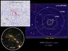 |
Fig. 1. Imaging and redshifts spatial distribution for MACS0416. On the top left, the VST i-band image, covering a central region of the cluster (30′ × 30′), is shown with MUSE (red) and VIMOS (blue) redshifts, over the range z = [0.02 − 6.2]. The bottom left image shows the Hubble Frontier Fields (HFF) color image (2.8′), where MUSE yields additional z in the cluster core. The right color composite image combines VST g- and i- plus the VISTA Ks- bands. |
Within the HFF investigation, with a high-resolution dissection of the two-dimensional total mass distribution in the core of MACS0416, Annunziatella et al. (2017) found no significant offset between the stellar and dark matter components within the core of the cluster. Moreover, Bonamigo et al. (2017) quantified the gas-to-total mass fraction at approximately 10% at a distance of 350 kpc from the cluster centre, demonstrating that the dark matter to total mass fraction remains relatively stable up to that distance. Recently, MACS0416 was observed by the James Webb Space Telescope (JWST) as part of the Prime Extragalactic Areas for Reionization and Lensing Science (PEARLS; Windhorst et al. 2023). These observations extended the wavelength range to approximately 5 μm, offering enhanced resolution and sensitivity in the infrared compared to previous HST data.
MACS0416 is also a focal point of the European Southern Observatory’s (ESO) Large Programme on Dark Matter Mass Distributions of Hubble Treasury Clusters and the Foundations of ΛCDM Structure Formation Models (CLASH-VLT; Rosati et al. 2014), utilizing the VIMOS data at the Very Large Telescope (VLT). In their study, Balestra et al. (2016), presenting the large spectroscopic campaign that provided ≥4000 reliable redshifts over ∼600 arcmin2 including ∼800 cluster member galaxies, confirmed the complex dynamical structure of the cluster, characterized by a double-peaked profile suggestive of a merging cluster, supporting the notion that the system is observed in a pre-collisional state, consistent with findings from radio and deep X-ray analyses by Ogrean et al. (2015). The velocity dispersion for each of these components was found to be  and
and  km s−1 (Ebeling et al. 2014; Jauzac et al. 2014). In the light of the above, the combination of photometric and spectroscopic data now available for MACS0416, derived from extensive HST, VLT, Chandra, and JWST observations, places it as one of the best datasets for investigating the dark matter distribution in a massive merging cluster through strong lensing techniques (Diego et al. 2024). Furthermore, MACS0416 also serves as an ideal laboratory for studying stellar populations and the effects of the environment on galaxy populations within massive clusters. Within the CLASH-VLT survey, Olave-Rojas et al. (2018), based on photometric and spectroscopic analysis, dynamically identified the two above-mentioned substructures within a radius less than 2R200 surrounding MACS0416. The authors also analysed galaxy colours to explore how pre-processing impacts the suppression (quenching) of star formation in these galaxies. By comparing the fractions of red (passive) and blue (star-forming) galaxies in the main cluster and its substructures, the authors observe consistent spatial trends since in both the main cluster and substructures, galaxies further from the cluster centre (r ≥ R200) show a smaller fraction of blue galaxies compared to field galaxies. Additionally, the study finds that at large distances, the quenching efficiency of substructures is similar to that observed in the main cluster, suggesting that pre-processing significantly influences galaxy evolution and quenching in these environments. The analysis highlights that pre-processing that occurs in the substructures is an important factor in the transition of galaxies into passive states at low redshifts. Finally, in a recent work by Estrada et al. (2023), the authors provide an in-depth analysis of galaxy assembly and the influence of the environment on the galaxy population within the massive cluster MACS0416. Using data obtained from the Galaxy Assembly as a Function of Mass and Environment with VST survey (VST-GAME survey, P.I. A. Mercurio), combined with VISTA data (G-CAV survey, P.I. M. Nonino) the study focuses on photometric analysis to explore the density field and structure of MACS0416, with particular attention to the outskirts of the cluster where signs of galaxy or galaxy group infall are detected. They apply photometric redshift techniques and galaxy classification methods not only to generate a robust catalogue of candidate cluster members, based on their photometric properties, but also to identify galaxy populations across different environments, including the dense core and the more diffuse outer regions of the cluster. The analysis reveals that the g − r colour distribution exhibits a bimodal pattern across all environments, with red galaxies displaying a shift towards redder colours as the environmental density increases. Conversely, the fraction of blue cloud galaxies increases as the environmental density decreases. The key findings of the study highlight the existence of three distinct overdensity structures in the outskirts of MACS0416 at approximately 5.5R200, suggesting the ongoing accretion of galaxy groups into the cluster, a clear indication of the pre-processing scenario. The authors conclude that these structures represent infalling groups, which may significantly contribute to the galaxy population in the cluster, affecting their subsequent evolution through environmental interactions. In terms of galaxy properties, the study finds that the galaxies within these overdensity regions exhibit mean densities and luminosities similar to those of the cluster core and different characteristics compared to those in the field. Their colours suggest that these galaxies may be part of evolved populations, providing further evidence for pre-processing effects acting on galaxies in these substructures. The analysis presented in this work constitutes a spectroscopic follow-up of the photometric sample by Estrada et al. (2023). Our main goal is to spectroscopically analyse the overdensity structures they identified in the outskirts of MACS0416, thus providing evidence of ongoing group infall into the cluster. This spectroscopic analysis will provide a more detailed understanding of the evolution of these substructures and their contribution to the pre-processing scenario. Additionally, we aim to qualitatively study the stellar populations as a function of g − r colour and K-band luminosity (as a proxy for the stellar mass), and within different environments of the cluster in terms of local density, shedding light on the influence of the cluster environment on galaxy evolution.
3. Observations, data reduction, and redshift measurement
The observations were conducted over four nights, from November 2 to November 5, 2021 (program ID: O/2021B/008, P.I. A. Mercurio), using the Two Degree Field (2dF) Multi-Object System (MOS) combined with the AAOmega Spectrograph mounted on the Anglo-Australian Telescope (2dF+AAOmega). During dark time and under clear weather conditions (seeingmax = 1.3″), six AAOmega MOS runs, each with an exposure time of 3 h (i.e. total exposure time ∼18 h), were planned to be carried out using different fibre configurations, but sharing the same centre. The goal was to achieve a signal-to-noise ratio (S/N) ≥ 5 for objects with a V-band magnitude limit of Vlim < 21.5 mag. Unfortunately, out of the ∼2000 galaxies initially expected, only ∼1290 targets were observed, that is ∼30% of the total number of objects in the photometric catalogue with Vlim < 21.5 mag. This shortfall was due to time lost because of bad weather, which affected two nights (i.e. 50% of the total allocated time). This incompleteness prevented us from fully spectroscopically covering all the photometric overdensities detected by Estrada et al. (2023) and partially limited the statistical significance of the sample. However, despite this limitation, our analysis remains robust and significant within the observed sample, supporting the scientific validity and relevance of our results (see Sect. 5). The 2dF+AAOmega Spectrograph data were acquired with the grating sets 385R and 580V, which cover the wavelength ranges from 370 nm to 580 nm (blue arm) and from 560 nm to 950 nm (red arm), respectively, with a resolution R = 1300 (Sharp et al. 2006).
We reduced the raw data and merged the spectra from the two arms using the standard 2dfdr pipeline1 v5.33 with default configuration and with the principal component analysis (PCA) that enabled the improvement of sky background subtraction. It is worth noting that the sky contribution was subtracted on the basis of only eight observed sky spectra, an insufficient number to accurately sample the sky across the entire FoV; this affects mainly the redder part of the spectra. For this reason, we applied cuts to the blue and red ends of each spectrum, excluding the low S/N range in the blue and the residuals of telluric absorptions in the red range. After these cuts, our 1290 spectra cover a wavelength range [3800−7300] Å (see Appendix A for more details about the data reduction). Among these, 24 spectra correspond to six galaxies with previously known redshifts, estimated using MUSE data (Caminha et al. 2017). These galaxies were repeatedly observed in each MOS configuration for calibration purposes. This leaves us with a final sample of 1272 unique spectra, of which 1266 correspond to new, previously unobserved objects (see Sect. 4 for details). Spectroscopic redshifts in this work were determined using two complementary methods: (1) an automatic redshift estimation tool called Redrock (Guy et al. 2023) and (2) visual inspection of all spectra to validate Redrock’s results and manually estimate the redshift when the automatic output was deemed unsatisfactory. In the latter case, the estimation was performed using the Pandora EZ software (Garilli et al. 2010). In Appendix B, both independent methods are described to provide a comprehensive overview of the procedures for obtaining spectroscopic redshifts. We also developed and implemented a new complementary software tool, Redmost2, designed for redshift determination. This tool allowed us to use Redrock for automatic redshift determination, while offering a graphical interface for real-time verification of the quality of the results produced by Redrock. In cases where the reliability of the automatic determination was low, and the estimation had not yet been refined with Pandora EZ, we were able to manually intervene and refine the redshift estimate similarly to EZ, as described in detail in Appendix B. In Fig. 2, we show the spectrum of one of the galaxies in our sample (at the average z of the cluster), where the redshift estimation by Redrock was done. The spectroscopic catalogue thus obtained is described in detail in Sect. 4. It is worth noting, at this stage of the analysis, that no absolute flux calibration has been applied to the spectra as this lies beyond the scope of the present work. However, for the purpose of an internal comparison between spectra aimed at showcasing the potential of our dataset, the lack of absolute flux calibration does not compromise the scientific value or potential of the sample.
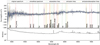 |
Fig. 2. In the top panel is shown the spectrum of a galaxy from our AAOmega sample (ID: MACS64052446, z ∼ 0.40), with the z estimated via Redrock. The key emission and absorption lines are marked with coloured dashed lines (see legend at top). The variance of the spectrum is illustrated in the bottom panel. |
4. The outskirts of MACS0416: AAOmega spectroscopic catalogue, selection of cluster members, and their redshift distribution
In this section we present the spectroscopic catalogue of the redshifts for the newly acquired objects. These additional sources in the field further enrich the already existing spectroscopic catalogue for this cluster (Balestra et al. 2016). After estimating the redshifts from the extracted spectra, we proceeded with a visual inspection to assign a quality flag (QF) to each redshift estimate, following the same criteria as Balestra et al. (2016) and Mercurio et al. (2021):
-
QF = 1: Uncertain redshift estimate. Low signal-to-noise ratio, which hinders the clear identification of spectral features, resulting in a reliability of ∼20−40%;
-
QF = 2: Redshifts are likely well estimated. Detection of at least two emission or absorption features, yielding an 80% reliability;
-
QF = 3: Reliable redshift estimate. Multiple emission lines and/or absorption features are identified, ensuring a 100% confidence level in the redshift measurement;
-
QF = 9: Emission line-based redshift estimation. One or (a few) more emission lines are detected, leading to a reliability of greater than 90%.
For 17 sources among the previously unobserved 1266 galaxies, no redshift estimate could be obtained. We successfully estimated redshifts for 1249 objects with a QF ≥ 1, resulting in a success rate of ≃98.7%. Within this subset, 13 objects were assigned a redshift quality flag QF = 1 (∼1%), 165 QF = 2 (∼13%), 1065 QF = 3 (∼84%), and 6 galaxies were flagged with QF = 9 (∼1%). Therefore, if we conservatively consider only those objects in our catalogue with a QF ≥ 2, which totals 1236 out of the original dataset of 1266 sources, the success rate corresponds to ≃97.6%. The resulting spectroscopic catalogue, which is publicly available at the CLASH-VLT website3, includes the information listed in Table 1 for the galaxies for which the redshift estimation is characterized by a QF ≥ 2. The spatial distribution of all objects included in the complete AAOmega catalogue, is shown in Fig. 3 overlaid on the wide-field i-band image from the VST telescope. Specifically, all 1236 of these objects with redshifts measured using AAOmega are represented in turquoise. These objects complement an existing catalogue of 4711 sources in the MACS0416 field, with redshifts previously estimated using VIMOS or MUSE instruments, limited to within ∼2R200. This VIMOS/MUSE region is shown in the figure with a blue rectangle. The AAOmega members (see Sect. 4) are shown as light blue circles with black edges. As shown in Fig. 3, it is worth highlighting that the AAOmega dataset allows us to probe cluster regions extending well beyond 5R200, corresponding to distances greater than 10 Mpc from the cluster centre. This extensive coverage provides the necessary means to achieve our primary goal: analysing the global properties of galaxies in the outskirts of MACS0416. The spectroscopic redshift distribution of the MACS0416 cluster field from the AAOmega catalogue is shown in panel a of Fig. 4. Only objects with redshift z ≤ 1 (1233 out of 1236) are displayed to enhance thevisualization of the statistical distribution of sources around the redshift (z = 0.397) of the cluster. Three galaxies have z ≥ 1, with values of z = 1.38, 2.76, 4.32. In the next section we provide the selection of the galaxies in our catalogue that belong to the cluster. A statistically significant peak of objects around the cluster redshift (z = 0.397) is evident in the distribution, indicating the detection of a significant number of objects belonging to the cluster between ∼2R200 and ∼5.5R200 in our AAOmega spectroscopic catalogue. These objects populate the cluster outskirts. Another significant peak is detected at z ∼ 0.30, likely representing a foreground structure that serendipitously falls within our FoV. In order to perform the selection of the spectroscopic cluster members, since the dynamical analysis of the cluster members is the subject of a forthcoming paper (Ragusa et al., in prep.), and it is beyond the scope of this study, here we focus on analysing the global properties of galaxies selected as spectroscopic fiducial members of the cluster. It was obtained adopting the redshift range z = [0.382−0.412], corresponding to Δz = 0.015, derived from the fiducial velocity range ±3000 km/s (i.e. Δz = 0.014, used in Balestra et al. 2016; Rosati et al. 2014) and accounting for the uncertainty in the cluster’s redshift centre (Δz = 0.001). Between z = 0.382 and z = 0.412, we identified a sample of 148 new members that populate the outskirts of MACS0416. Hereafter, the term cluster members refers generically to galaxies within the redshift range z = [0.382 − 0.412], including different populations such as potential infalling or backsplash galaxies since a detailed dynamical analysis will be presented in a forthcoming work. The redshift distribution of these new objects, shown in panel b of Fig. 4. We recover the same statistically significant redshift peaks previously identified in the VIMOS sample (Balestra et al. 2016), with the AAOmega data independently reinforcing the robustness and reliability of these
New catalogue of spectroscopic redshift of MACS0416 field obtained with AAOmega observations.
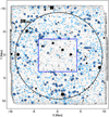 |
Fig. 3. VST i-band image covering 1 deg2 (∼20 × 20 Mpc2), overlapped with the 1236 AAOmega measured redshifts (turquoise points). The light blue circles with black edges represent the new 148 members of MACS0416 from AAOmega catalogue, in the redshift range z = [0.382 − 0.412]. The region where VIMOS or MUSE redshifts are available over z = [0.02 − 6.2] range is represented as a blue rectangle. The black circle corresponds to the radial distance from the cluster centre of 5R200 ∼ 9.1 Mpc. |
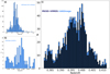 |
Fig. 4. Top left panel: Redshift distribution of the 1233 sources extracted from the AAOmega spectra. Three objects with redshift ≥1 were excluded from the plot for a better visualization of the distribution. Bottom left panel: Zoomed-in image of the redshift range of the members selected with AAOmega observations. Right panel: Redshift distribution of the 1017 from MUSE or VIMOS (blue) plus 148 from AAOmega (turquoise) spectroscopic cluster members selected in the range z = [0.382−0.412]. |
structures. The highest peak is around the cluster’s mean redshift (z = 0.397). Additionally, smaller peaks, such as the one around z = 0.384, are also observed. These may correspond to the overdense regions (i.e. groups undergoing infall, namely pre-processing) that we aim to identify (see Sect. 5.3). In the panel c of Fig. 4, the statistical distribution of the entire redshift sample available in the MACS0416 field (a total of 1165 objects) within the redshift range z = [0.382 − 0.412] is shown. This distribution was obtained by expanding the previously observed sample (in blue) with the addition of 148 new reliable AAOmega member galaxies (in turquoise). Moreover, the secondary peaks around z ∼ 0.384 and z ∼ 0.405, already partially visible in the redshift distribution of the AAOmega sample, appear even more pronounced in the total catalogue MUSE+VIMOS+AAOmega. In the following section we analyse the member galaxies’ global features from the AAOmega spectroscopic dataset to characterize their average physical properties.
5. A complete census of MACS0416
In this work, we present the 2dF+AAOmega spectroscopic dataset of the galaxy cluster MACS0416 at z = 0.397, focusing on its peripheral regions. This enabled the study of spectral properties’ relationships with the cluster environment, including the detection of overdensities and filamentary regions, photometrically detected by Estrada et al. (2023). The available optical and NIR catalogues enable a comprehensive characterization of galaxies down to the dwarf scale (M⋆ ∼ 109 M⊙). These combined datasets will serve as an invaluable resource for studying galaxy evolution across a broad range of environments, from the core of the cluster to its outskirts at ∼5.5R200, and offer an opportunity to explore galaxy properties and mass assembly at intermediate redshift (z ∼ 0.4), providing insights that cannot be matched by studies of other clusters at similar redshifts.
5.1. The tale of red and blue galaxies: Colour dependence of galaxy properties
Building upon the work in Sect. 4, we matched our sample to the Estrada et al. (2023) photometric catalogue and used the galaxy (g − r)Kron colour (i.e. the g − r colour inside an aperture of one Kron radius) to separate the blue and red galaxies. We adopted the colour cut founded by Estrada et al. (2023), i.e. (g − r)Kron ∼ 1.20 mag. We also corrected the magnitudes for the Galactic extinction using the extinction coefficients provided by Schlafly & Finkbeiner (2011). In this way, we obtained 72 red and 76 blue galaxies. At this early stage, the classification relied solely on the observed (g − r)Kron colour, without yet incorporating any spectral property. As a first qualitative result of this analysis, and as evident from this simple colour cut, we observe that, contrary to expectations (the so-called morphological segregation or morphology-density relation; e.g. Oemler 1974; Dressler 1980; Vulcani et al. 2023), the number of blue galaxies was not significantly higher than that of red galaxies. Instead, both populations appeared to be comparable in number within our sample. This seems to suggest that we are likely observing galaxies that reside in more evolved structures in the outskirts, tracing regions of higher environmental density in the periphery of MACS0416. In the left panel of Fig. 5 we show the average spectral properties of our sample as a function of colour; in black is the average spectrum of all 148 AAOmega members of MACS0416, in red that of all the 72 red galaxies, and in blue the average spectrum of all 76 blue galaxies, following the colour cut described above. All the spectra have been shifted to the rest frame and smoothed with a Gaussian kernel with a sigma of 2 pixels. Moreover, the colour distribution of our sample is illustrated in the inset in the top left corner of the left panel of Fig. 5, where the x-axis represents the observed (g − r)Kron colour corrected for extinction. We have colour-coded the galaxies in the distribution according to the colour cut defined above, specifically highlighting the distribution of blue galaxies (in blue) and red galaxies (in red). As expected, red and blue galaxies show significant spectral differences due to their varying star formation (SF) activities. Red galaxies are typically old passive systems with little to no ongoing star formation, and are called early-type galaxies (ETGs). These galaxies tend to exhibit prominent absorption features in their spectra from heavy elements, for example calcium (Ca, particularly prominent is the calcium CaIIH and CaIIK absorption lines doublet), iron (Fe), and magnesium (Mg), reflecting the contribution of old star populations. Mostly prominent in passive galaxies is then the Balmer break, a discontinuity in the spectral continuum, seen around 4000 Å in the rest frame, that can be used as a key indicator of the age of the stellar population in a galaxy (Bruzual & Charlot 2003; Kauffmann et al. 2003; Gallazzi et al. 2005; Franzetti et al. 2007). In contrast, the blue and star-forming galaxies, also known as late-type galaxies (LTGs), are actively forming stars, and are characterized by prominent emission lines in the spectrum, such as the [OII]λ3727, [OIII]λ5007−4959 doublet, Hβ, Hα. These differences in the galaxy populations are crucial for understanding galaxy evolution as they reflect different stellar ages, different star formation histories, and different gas content in galaxies, and they serve as important indicators for classifying galaxies and understanding their role within the cosmic web of large-scale structures. In our sample, the stacked spectrum of the entire AAOmega sample (in black, left panel of Fig. 5) reveals distinct features indicative of a young stellar population, reflecting mostly the features of the blue galaxies (in blue, left panel of Fig. 5) such as the strong emission lines of [OII], [OIII], and Hβ, which are consistent with galaxies typically found in the outer parts of clusters or field. Such galaxies are often in the process of falling into a cluster or have recently undergone this process, making them less affected by environmental effects compared to those residing in the denser cluster core. On the other hand, fully consistent with expectations, the average spectrum of the red galaxies (in red, left panel of Fig. 5) shows several distinct absorption features, especially the sharply defined CaIIH and CaIIK absorption lines and G-band, which can typically be observed in old and more evolved stellar systems. This red population can serve as an efficient tracer of the cosmic web, starting from the filamentary structures that correspond to the areas where the cluster is accreting smaller systems, such as other galaxies or groups. In summary, from the qualitative analysis of the spectral lines emerging from our stacked spectra, we can distinguish the different properties described above and reconstruct the general colour bimodality behaviour of the galaxies. In each plot in this work, we also highlighted with a shaded vertical grey area, the spectral region corresponding to the joining between the blue and red arms. This region includes the Hδ line, which is therefore excluded from our analysis, both in emission and in absorption. A detailed study of this feature will be presented in a forthcoming paper (Ragusa et al., in prep.) as an accurate flux calibration is required in that wavelength range.
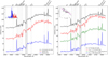 |
Fig. 5. Average spectral properties of our sample as a function of colour and KKron as a proxy of the stellar mass. Left panel: Sample divided into red (72) and blue (76) galaxies, with their stacked spectra displayed in red and blue, respectively. A (g − r)Kron colour cut was used. The inset in the top left corner shows a colour distribution of our sample, where the x-axis represents the observed (g − r)Kron colour, corrected for extinction. Right panel: Whole sample divided into three subclasses based on the three bins of KKron. In red is the stacked spectrum of the brightest galaxies with KKron < 17.9 mag, in green that of the galaxies with intermediate luminosity 17.9 mag ≤ KKron < 18.9 mag, and in blue the stacked spectrum of the faint galaxies with KKron ≥ 18.9 mag. In the top left corner, an inset showing the trend between (g − r)Kron and KKron magnitude is reported. The dashed magenta line corresponds to the best fit of the linear correlation. In both panels, the stacked spectrum of the entire population of members (148) of MACS0416, obtained with AAOmega, is shown in black. All spectra are rest-frame and have been smoothed using a Gaussian kernel with a sigma of 2 pixels. The vertical dashed grey area corresponds to the spectral region of the join between the two arms. |
5.2. Mass dependence of spectral properties
It is well known that a galaxy’s mass strongly affects its evolution (e.g. Thomas et al. 2010). In this section we discuss the spectral properties of our sample galaxies as a function of their K-band luminosity used as a proxy of their stellar mass. The K-band magnitude is a widely used proxy for estimating the stellar mass of galaxies (e.g. Gavazzi et al. 1996; Kauffmann & Charlot 1998; Sureshkumar et al. 2021). This is primarily because there is a relatively tight correlation between K-band luminosity and stellar mass, assuming a reasonable stellar mass-to-light ratio (M/L) (e.g. de Jong & Bell 2001). Moreover, the light in the NIR region is less affected by dust extinction compared to optical bands, and more directly traces the light emitted by older more evolved stars, particularly red giants, providing a more accurate assessment of stellar luminosity (e.g. Verheijen 2001; Kauffmann et al. 2003; Sureshkumar et al. 2023). Our objective here is to use the K-band magnitude within the Kron radius (KKron), as provided by Estrada et al. (2023), to classify the cluster member galaxies within our sample as bright or faint. To this end, we divided our sample into three bins based on KKron, defined as follows: (i) KKron ≤ 17.9 mag (48 galaxies), (ii) 17.9 mag < KKron < 18.9 mag (51 galaxies), and (iii) KKron ≥ 18.9 mag (49 galaxies). These bins were specifically chosen to ensure a uniform distribution of galaxies across each category, facilitating a balanced comparison of their spectral properties across different magnitude (mass) ranges, taking into account that we selected these three KKron bins with similar widths within our sample to ensure a consistent level of completeness across them. The right panel of Fig. 5 illustrates the rest-frame stacked spectra for each defined subsample, smoothed with a Gaussian kernel with a sigma of 2 pixels. From top to bottom, it includes the mean spectrum of the entire population of cluster members (in black), followed by the spectra of the bright galaxy population (in red), the intermediate-luminosity galaxy population (in green), and finally, the faintest galaxy population (in blue). Moreover, an inset showing the trend between (g − r)Kron and KKron magnitude is reported in the top left corner, confirming that, as expected, redder colours correspond to brighter and therefore more massive galaxies. From a purely qualitative point of view, the spectral properties of galaxies in our sample vary systematically with KKron (so with the stellar mass). High-mass galaxies (red spectrum) exhibit strong absorption features (see Sect. 5.1 for details) with a relatively faint emission lines (such as the [OII] line), suggesting more probably an incomplete quenching scenario. The spectrum of intermediate-mass galaxies (green) shows both emission (i.e. [OII], [OIII], Hβ) and absorption (i.e. CaII doublet, G-band, Hδ) features, suggesting a transitional population with ongoing star formation. Of particular interest is the observed inverted ratio, in the green spectrum, between the two CaII lines compared to that observed in the red spectrum, typical of galaxies that have recently stopped their star formation activity. For galaxies dominated by older stars, the CaIIK line typically shows a stronger absorption than the CaIIH line, resulting in an H:K ratio lower than 1, as demonstrated in studies such as Rose (1984, 1985). The H:K ratio is particularly sensitive to the presence of stellar populations younger than ∼200 My (Moresco et al. 2018) since young stars produce absorption in Hϵ that overlaps with CaIIH. Finally, the spectrum of low-mass galaxies (blue spectrum) is dominated by strong emission lines, particularly [O II], [O III], Hβ, Hγ, and Hϵ, the last filling in the CaIIH absorption, indicating active star formation and younger stellar populations. In general, as highlighted by the average spectrum of the entire sample (black spectrum), the most prominent feature is that the overall galaxy population exhibits characteristics of younger stellar populations compared to the old galaxies typically found in the cores of the clusters. Given that the dataset is focused on the outskirts of the cluster, this suggests that it likely includes galaxies that have not yet been fully quenched by the environment. These galaxies are presumably in a phase where they are still experiencing star formation or have only recently ceased their star-forming activity. These results support the idea that dividing our sample based on K-band magnitude, and, by extension, galaxy stellar mass, enables the identification of distinct stellar populations. Notably, the less luminous subsample exhibits features indicative of younger stellar populations. This aligns with the expected behaviour of galaxies in cluster outskirts, which are often not yet quenched and may experience ongoing or recent star formation bursts, as observed in post-starburst systems. The spectral analysis highlighted in this study provides qualitative insights into the connection between galaxy stellar population properties and their mass, and we defer the detailed analysis of the spectral indicators in a quantitative way to the upcoming paper (Ragusa et al., in prep.). This follow-up analysis will aim to elucidate the mechanisms governing galaxy evolution within the whole cluster environment.
5.3. Galaxies at the edge: Environmental dependence of galaxy properties
In this section we analyse the spectral properties of galaxies in the outskirts of the galaxy cluster MACS0416, following the environmental density definition by Estrada et al. (2023), who found three overdensity regions in the cluster periphery, and also evidenced that the properties of galaxies vary as the field density changes. As a preliminary step in our analysis of overdensities in the outskirts, used as tracers of galaxy groups undergoing infall into the cluster, in the left panel of Fig. 6 we superimpose the whole AAOmega dataset on the density field of objects identified as cluster members through photometric SED fitting Estrada et al. (2023). The light blue dots correspond to spectroscopically confirmed members, while the white ones represent sources observed during the AAOmega spectroscopic runs but later found not to belong to the cluster. In the right panel of Fig. 6 we have highlighted the overdensity regions A, B, and C photometrically identified by Estrada et al. (2023), including the filamentary structures, and overlaid our spectroscopically confirmed members, colour-coded according to the density of the environment in which they reside: red for overdense regions, green for filamentary regions, and blue for underdense areas. As suggested by the right panel of Fig. 6, the spectroscopic follow-up appears to trace very well the overdense region B and the entire filamentary structure connecting region B to region C. Interestingly, the galaxies that trace region B also constitute the secondary peak observed in the redshift distribution (see panel 4b in Fig. 4) around z ∼ 0.385. Similarly, those tracing the filamentary structures surrounding region C appear to contribute to another secondary peak at z ∼ 0.405. These findings support the hypothesis that such structures may correspond to real physical systems currently experiencing infall into the main body of the cluster. Region A, on the other hand, does not seem to have a well-defined spectroscopically confirmed counterpart, although it exhibits the highest photometric density. This is primarily because the photometric member candidates in this region did not meet the magnitude limit imposed by our spectroscopic sample selection, particularly in its more crowded inner area. In total, we spectroscopically confirm 81 galaxies in the three overdensities, A, B, and C, plus filamentary regions. To characterize the local environment, we divided the sample of confirmed members into three distinct bins based on local density information (for details on how the mean density δ was calculated, see Sect. 5.2 of Estrada et al. 2023): low (δ ≤ 0), medium (0 < δ ≤ 1), and high (δ > 1) density. The first interval represents underdense regions, where the local density is below the mean value across the observed FoV. The second interval corresponds to overdense regions with local densities ranging up to twice the mean value (corresponding to the filamentary regions), while the third interval identifies the regions with the highest density values observed within the field (i.e. the overdensities). In Fig. 7 we show the stacked spectra of all the objects that fall into the specific bin of overdensity smoothed with a Gaussian kernel with a sigma of 2 pixels: (i) in red is the average spectrum for the galaxies within the overdensities (δ > 1); (ii) in green that of galaxies located in the filamentary regions (0 < δ ≤ 1); (iii) in blue that of the galaxies located in underdense regions (δ ≤ 0). As usual, in black we insert the stacked spectrum of all the members. Moreover, the bottom panels show on the left the (g − r)Kron and on the right the KKron distributions for each δ class (i.e. −1, 0, 1), confirming that on average, as expected, redder colours correspond to galaxies inhabiting denser local environments and that the KKron distributions in the three δ bins are fully consistent. Following the same (g − r)Kron colour cut defined in Sect. 5.1, we divided the sample into red and blue galaxies. To analyse the global spectral behaviour of red and blue galaxies across varying local environments, for each subclass, we plot their spectral properties as a function of the local density, consistent with the scheme described in Fig. 7. Specifically, the left panel of Fig. 8 presents the smoothed stacked spectrum (using a Gaussian kernel with a sigma of 2 pixels) of the red population as a function of δ where a progressively darker red colour corresponds to increasing δ. Similarly, the right panel of Fig. 8 displays the corresponding trend for blue galaxies, where the intensity of blue shading increases with rising δ. Additionally, at the top of each panel, we include, for comparative purposes, the stacked and smoothed spectra of the total population of red galaxies and blue galaxies. As anticipated and extensively discussed in Sects. 5.1 and 5.2, Figs. 7 and 8 clearly show that, as the local density increases, galaxies tend to become progressively redder, more massive, and more quenched. This trend is observed even though our sample mainly consists of galaxies located in the outskirts of the cluster (i.e. out of the 148 member galaxies, 145 are located beyond 2R200), where environmental quenching is not yet fully completed. Evidence of ongoing star formation is also apparent in the stacked spectrum of galaxies in the densest areas (see Fig. 7), where non-negligible emission lines persist. Specifically, the left panel of Fig. 8 shows that red galaxies in overdense regions exhibit more passive behaviour than their lower-density counterparts, likely indicating a more evolved stellar population. This is evident from the higher H:K ratio, and the more pronounced Balmer break around 4000 Å observed in the transition from lower-density red galaxies (yellow spectrum in the left panel of Fig. 8) to those in the overdensities (red spectrum in the left panel of Fig. 8). Conversely, a younger population of blue galaxies, which are less massive and significantly more active, predominantly occupy regions of lower local density (blue spectrum in Fig. 7). This supports the idea that galaxy quenching is primarily driven by environmental effects, being more pronounced in areas of higher density. Notably, when analysing only the blue galaxy sample (right panel of Fig. 8), their spectral properties show minimal variation as a function of the environmental density. This homogeneity suggests that these galaxies likely represent a younger population that has undergone a relatively recent infall and has not yet had sufficient time to experience the full effects of the cluster environment. As expected, the number of blue galaxies in the high-density regions is significantly low (N = 3). It is worth mentioning that we also performed Kolmogorov–Smirnov (KS) tests between each pair of K-band magnitude distributions for the galaxy populations shown in both the left and right panels of Fig. 8. In this case, we obtained p-values significantly greater than 0.05 (on average around 0.5), confirming that the K-band magnitude distributions of the different populations are statistically compatible, as already shown in the bottom right panel of Fig. 7. This supports the idea that the spectral differences shown in Fig. 8 are not primarily driven by stellar mass, but rather reflect genuine environmental effects. In summary, we spectroscopically confirm 81 out of 148 galaxies belonging to regions identified by Estrada et al. (2023) as filamentary or overdense areas. These galaxies are likely to have either recently experienced infall into the cluster (overdense regions) or are currently undergoing infall (filamentary regions), either as individual galaxies or as part of galaxy groups. As extensively discussed in Sect. 5.2, mass is also a fundamental driver for quenching mechanisms. Separating the effects of mass and environment will be the focus of a forthcoming paper (Ragusa et al., in prep.) as it will require combining the VIMOS, MUSE, and AAOMEGA datasets, which will together provide a total of over 1000 members, allowing us to analyse these effects and the physical properties of the different galaxy populations in a statistically complete way.
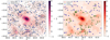 |
Fig. 6. Left panel: Photometric density map of MACS0416 from Estrada et al. (2023), with all the new redshifts of objects with QF ≥ 2 (1236) obtained with AAOmega overlaid (white circles), highlighting the new spectroscopic cluster members (148) (light blue circles). Right panel: Same as left panel, with all the new spectroscopic cluster members (148) obtained with AAOmega overlaid, colour-coded as a function of δ. The red and green points are the members in the overdensities plus filamentary structures, while blue points are those in the underdense regions. |
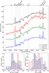 |
Fig. 7. Average spectral properties of our sample as a function of the local environment. Top panel: Stacked spectrum of the AAOmega members (148) is shown in black. The stacked spectra of galaxies located in overdense regions are shown in red; those in filamentary regions in green; and those in less dense areas, comparable to the field, in blue. All spectra are rest-frame and have been smoothed using a Gaussian kernel with a sigma of 2 pixels. The vertical dashed grey area corresponds to the spectral region of the join between the two arms. Bottom panels: (g − r)Kron (left) and KKron (right) distributions of the galaxies in our sample as a function of the same three δ bins (red, green, and blue). |
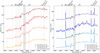 |
Fig. 8. Average spectral properties of our sample of red and blue galaxies as a function of the local environment. Left panel: Stacked spectrum of the population of red members (72) of MACS0416, is shown in dark red, at the top of the image. The entire sample was then divided into three subclasses based on the three bins of density δ. The stacked spectra of the red galaxies located in overdense regions are shown in red; those in filamentary regions in coral; and those in less dense areas, comparable to the field, in orange. Right panel: Same as the left panel, for the blue members (76) of MACS0416. All spectra are rest-frame and have been smoothed using a Gaussian kernel with a sigma of 2 pixels. The vertical dashed grey area corresponds to the spectral region of the join between the two arms. We performed a Kolmogorov–Smirnov (KS) test on each pair of average spectra in the left and the right panels, obtaining p-values much smaller than 0.05 (effectively consistent with zero), which strongly supports our assumption that the average spectra of the different populations are statistically distinct. |
6. Conclusions
In this study we have provided a comprehensive analysis of the outskirts of the galaxy cluster MACS0416, extending our investigation to a remarkable distance of ∼5.5R200 (i.e. ∼10 Mpc). Building on the photometric data previously obtained by Estrada et al. (2023), we have complemented this dataset with newly acquired spectroscopic observations using the AAOmega multi-object spectrograph. The large FoV and multiplexing capabilities of AAOmega allowed us to obtain robustly estimated redshifts for 1236 unique objects inhabiting the FoV of the cluster outskirts. This unprecedented dataset has facilitated a detailed exploration of the environmental processes influencing galaxy evolution in these peripheral regions. This work extends and complements the spectroscopic catalogue previously obtained using MUSE and VIMOS data, which covered regions up to 2R200 (Ebeling et al. 2014; Balestra et al. 2016; Caminha et al. 2017). From the spectroscopic analysis, we have constructed a catalogue of redshifts for all observed objects, identifying 148 as cluster members in the outskirts of MACS0416. These spectroscopic members provide critical insights into the environmental and evolutionary processes at play. By leveraging this dataset, we analysed the qualitative trends in galaxy spectral properties as a function of key parameters: the colour, the K-band magnitude (used as a mass proxy) and the local environmental density. This investigation revealed clear correlations between the environment and galaxy properties, particularly highlighting the significant role of overdensities and filamentary regions. A key finding of our work is the identification of 81 galaxies associated with both overdensities and filamentary structures previously identified by Estrada et al. (2023). These results strongly support the pre-processing scenario, where infall through the filaments of pre-assembled substructures, such as galaxy groups, plays a dominant role in the mass assembly history of the cluster. Galaxies in high-density environments exhibit spectralcharacteristics indicative of more massive, red, and passive populations, with colours comparable to those of the core galaxies (Estrada et al. 2023). In contrast, galaxies in low-density environments tend to be bluer, less massive, and more actively star-forming. These results highlight the transformative role of the environment, particularly in regions of higher density, where quenching mechanisms are more pronounced. Moreover, these findings underscore the importance of pre-processing phenomena in shaping galaxy properties before they enter into the cluster influence, and so contribute significantly to the mass assembly and star formation histories of cluster galaxies. This is evident from the presence of evolved stellar populations in the overdense regions, where galaxies show enhanced spectral features such as the Balmer break and CaH and CaK absorption lines. Conversely, the spectral properties of blue galaxies remain relatively uniform across environments, suggesting a younger less evolved population that has not yet been fully subjected to environmental effects, likely due to a more recent infall. The findings of this study are a preliminary but crucial step in advancing our understanding of the role of the environment in galaxy evolution. The work presented here will be complemented by a forthcoming detailed and quantitative analysis of the stellar populations of these galaxies (Ragusa et al., in prep.).
2dfdr is an automatic data reduction pipeline dedicated to reducing multi-fibre spectroscopy data from the AAT facility. For more information, see https://aat.anu.edu.au/science/software/2dfdr
References
- Annunziatella, M., Mercurio, A., Biviano, A., et al. 2016, A&A, 585, A160 [NASA ADS] [CrossRef] [EDP Sciences] [Google Scholar]
- Annunziatella, M., Bonamigo, M., Grillo, C., et al. 2017, ApJ, 851, 81 [NASA ADS] [CrossRef] [Google Scholar]
- Astropy Collaboration (Price-Whelan, A. M., et al.) 2022, ApJ, 935, 167 [NASA ADS] [CrossRef] [Google Scholar]
- Balestra, I., Mercurio, A., Sartoris, B., et al. 2016, ApJS, 224, 33 [Google Scholar]
- Balogh, M. L., Navarro, J. F., & Morris, S. L. 2000, ApJ, 540, 113 [Google Scholar]
- Battaglia, N., Bond, J. R., Pfrommer, C., & Sievers, J. L. 2012, ApJ, 758, 74 [NASA ADS] [CrossRef] [Google Scholar]
- Bergamini, P., Grillo, C., Rosati, P., et al. 2023, A&A, 674, A79 [NASA ADS] [CrossRef] [EDP Sciences] [Google Scholar]
- Biffi, V., Planelles, S., Borgani, S., et al. 2018, MNRAS, 476, 2689 [Google Scholar]
- Bonamigo, M., Grillo, C., Ettori, S., et al. 2017, ApJ, 842, 132 [NASA ADS] [CrossRef] [Google Scholar]
- Bonamigo, M., Grillo, C., Ettori, S., et al. 2018, ApJ, 864, 98 [Google Scholar]
- Bruzual, G., & Charlot, S. 2003, MNRAS, 344, 1000 [NASA ADS] [CrossRef] [Google Scholar]
- Caminha, G. B., Grillo, C., Rosati, P., et al. 2017, A&A, 600, A90 [NASA ADS] [CrossRef] [EDP Sciences] [Google Scholar]
- Chirivì, G., Suyu, S. H., Grillo, C., et al. 2018, A&A, 614, A8 [NASA ADS] [CrossRef] [EDP Sciences] [Google Scholar]
- Cowie, L. L., & Songaila, A. 1977, Nature, 266, 501 [Google Scholar]
- D’Addona, M. 2024, https://doi.org/10.5281/zenodo.10818017 [Google Scholar]
- Danovich, M., Dekel, A., Hahn, O., & Teyssier, R. 2012, MNRAS, 422, 1732 [Google Scholar]
- de Jong, R. S., & Bell, E. F. 2001, ASP Conf. Ser., 230, 555 [Google Scholar]
- De Lucia, G., Springel, V., White, S. D. M., Croton, D., & Kauffmann, G. 2006, MNRAS, 366, 499 [NASA ADS] [CrossRef] [Google Scholar]
- Dekel, A., Birnboim, Y., Engel, G., et al. 2009, Nature, 457, 451 [Google Scholar]
- Diego, J. M., Adams, N. J., Willner, S. P., et al. 2024, A&A, 690, A114 [NASA ADS] [CrossRef] [EDP Sciences] [Google Scholar]
- Diemer, B., Mansfield, P., Kravtsov, A. V., & More, S. 2017, ApJ, 843, 140 [NASA ADS] [CrossRef] [Google Scholar]
- Dressler, A. 1980, ApJ, 236, 351 [Google Scholar]
- Ebeling, H., Edge, A. C., & Henry, J. P. 2001, ApJ, 553, 668 [Google Scholar]
- Ebeling, H., Ma, C.-J., & Barrett, E. 2014, ApJS, 211, 21 [NASA ADS] [CrossRef] [Google Scholar]
- Estrada, N., Mercurio, A., Vulcani, B., et al. 2023, A&A, 671, A146 [NASA ADS] [CrossRef] [EDP Sciences] [Google Scholar]
- Flaugher, B., & Bebek, C. 2014, Proc. SPIE, 9147, 91470S [NASA ADS] [CrossRef] [Google Scholar]
- Franzetti, P., Scodeggio, M., Garilli, B., et al. 2007, A&A, 465, 711 [NASA ADS] [CrossRef] [EDP Sciences] [Google Scholar]
- Fujita, Y. 2004, PASJ, 56, 29 [NASA ADS] [Google Scholar]
- Gallazzi, A., Charlot, S., Brinchmann, J., White, S. D. M., & Tremonti, C. A. 2005, MNRAS, 362, 41 [Google Scholar]
- Garilli, B., Fumana, M., Franzetti, P., et al. 2010, PASP, 122, 827 [Google Scholar]
- Gavazzi, G., Pierini, D., & Boselli, A. 1996, A&A, 312, 397 [NASA ADS] [Google Scholar]
- Gnedin, O. Y. 2003, ApJ, 582, 141 [Google Scholar]
- Grillo, C., Suyu, S. H., Rosati, P., et al. 2015, ApJ, 800, 38 [Google Scholar]
- Gunn, J. E., & Gott, J. R. 1972, ApJ, 176, 1 [NASA ADS] [CrossRef] [Google Scholar]
- Guy, J., Bailey, S., Kremin, A., et al. 2023, AJ, 165, 144 [NASA ADS] [CrossRef] [Google Scholar]
- Hahn, C., Wilson, M. J., Ruiz-Macias, O., et al. 2023, AJ, 165, 253 [CrossRef] [Google Scholar]
- Hoag, A., Huang, K. H., Treu, T., et al. 2016, ApJ, 831, 182 [Google Scholar]
- Ichikawa, K., Matsushita, K., Okabe, N., et al. 2013, ApJ, 766, 90 [Google Scholar]
- Jauzac, M., Clément, B., Limousin, M., et al. 2014, MNRAS, 443, 1549 [Google Scholar]
- Jauzac, M., Jullo, E., Eckert, D., et al. 2015, MNRAS, 446, 4132 [Google Scholar]
- Kauffmann, G., & Charlot, S. 1998, MNRAS, 297, L23 [NASA ADS] [CrossRef] [Google Scholar]
- Kauffmann, G., Colberg, J. M., Diaferio, A., & White, S. D. M. 1999a, MNRAS, 303, 188 [NASA ADS] [CrossRef] [Google Scholar]
- Kauffmann, G., Colberg, J. M., Diaferio, A., & White, S. D. M. 1999b, MNRAS, 307, 529 [NASA ADS] [CrossRef] [Google Scholar]
- Kauffmann, G., Heckman, T. M., White, S. D. M., et al. 2003, MNRAS, 341, 33 [Google Scholar]
- Larson, R. B., Tinsley, B. M., & Caldwell, C. N. 1980, ApJ, 237, 692 [Google Scholar]
- Lau, E. T., Kravtsov, A. V., & Nagai, D. 2009, ApJ, 705, 1129 [NASA ADS] [CrossRef] [Google Scholar]
- Lau, E. T., Nagai, D., Avestruz, C., Nelson, K., & Vikhlinin, A. 2015, ApJ, 806, 68 [NASA ADS] [CrossRef] [Google Scholar]
- Levi, M., Bebek, C., Beers, T., et al. 2013, ArXiv e-prints [arXiv:1308.0847] [Google Scholar]
- Lotz, J. M., Koekemoer, A., Coe, D., et al. 2017, ApJ, 837, 97 [Google Scholar]
- Mann, A. W., & Ebeling, H. 2012, MNRAS, 420, 2120 [NASA ADS] [CrossRef] [Google Scholar]
- Mansfield, P., Kravtsov, A. V., & Diemer, B. 2017, ApJ, 841, 34 [NASA ADS] [CrossRef] [Google Scholar]
- Mercurio, A., Rosati, P., Biviano, A., et al. 2021, A&A, 656, A147 [NASA ADS] [CrossRef] [EDP Sciences] [Google Scholar]
- Meštrić, U., Vanzella, E., Zanella, A., et al. 2022, MNRAS, 516, 3532 [CrossRef] [Google Scholar]
- Mihos, J. C. 2004, in Clusters of Galaxies: Probes of Cosmological Structure and Galaxy Evolution, eds. J. S. Mulchaey, A. Dressler, & A. Oemler, 277 [Google Scholar]
- Mihos, J. C., & Hernquist, L. 1996, ApJ, 464, 641 [Google Scholar]
- Mirakhor, M. S., & Walker, S. A. 2021, MNRAS, 506, 139 [NASA ADS] [CrossRef] [Google Scholar]
- Moore, B., Lake, G., & Katz, N. 1998, ApJ, 495, 139 [Google Scholar]
- Moresco, M., Jimenez, R., Verde, L., et al. 2018, ApJ, 868, 84 [NASA ADS] [CrossRef] [Google Scholar]
- Mulchaey, J. S., & Zabludoff, A. I. 1998, ApJ, 496, 73 [NASA ADS] [CrossRef] [Google Scholar]
- Nagai, D., & Lau, E. T. 2011, ApJ, 731, L10 [NASA ADS] [CrossRef] [Google Scholar]
- Oemler, A. 1974, ApJ, 194, 1 [Google Scholar]
- Ogrean, G. A., van Weeren, R. J., Jones, C., et al. 2015, ApJ, 812, 153 [NASA ADS] [CrossRef] [Google Scholar]
- Ogrean, G. A., van Weeren, R. J., Jones, C., et al. 2016, ApJ, 819, 113 [Google Scholar]
- Olave-Rojas, D., Cerulo, P., Demarco, R., et al. 2018, MNRAS, 479, 2328 [Google Scholar]
- Paccagnella, A., Vulcani, B., Poggianti, B. M., et al. 2016, ApJ, 816, L25 [NASA ADS] [CrossRef] [Google Scholar]
- Paccagnella, A., Vulcani, B., Poggianti, B. M., et al. 2017, ApJ, 838, 148 [NASA ADS] [CrossRef] [Google Scholar]
- Paccagnella, A., Vulcani, B., Poggianti, B. M., et al. 2019, MNRAS, 482, 881 [NASA ADS] [CrossRef] [Google Scholar]
- Poggianti, B. M., Smail, I., Dressler, A., et al. 1999, ApJ, 518, 576 [Google Scholar]
- Postman, M., Coe, D., Benítez, N., et al. 2012, ApJS, 199, 25 [Google Scholar]
- Ragusa, R., Spavone, M., Iodice, E., et al. 2021, A&A, 651, A39 [NASA ADS] [CrossRef] [EDP Sciences] [Google Scholar]
- Ragusa, R., Mirabile, M., Spavone, M., et al. 2022, Front. Astron. Space Sci., 9, 852810 [CrossRef] [Google Scholar]
- Ragusa, R., Iodice, E., Spavone, M., et al. 2023, A&A, 670, L20 [NASA ADS] [CrossRef] [EDP Sciences] [Google Scholar]
- Raichoor, A., Moustakas, J., Newman, J. A., et al. 2023, AJ, 165, 126 [NASA ADS] [CrossRef] [Google Scholar]
- Richard, J., Jauzac, M., Limousin, M., et al. 2014, MNRAS, 444, 268 [Google Scholar]
- Roncarelli, M., Ettori, S., Borgani, S., et al. 2013, MNRAS, 432, 3030 [NASA ADS] [CrossRef] [Google Scholar]
- Rosati, P., Balestra, I., Grillo, C., et al. 2014, The Messenger, 158, 48 [NASA ADS] [Google Scholar]
- Rose, J. A. 1984, AJ, 89, 1238 [NASA ADS] [CrossRef] [Google Scholar]
- Rose, J. A. 1985, AJ, 90, 1927 [NASA ADS] [CrossRef] [Google Scholar]
- Rudd, D. H., & Nagai, D. 2009, ApJ, 701, L16 [NASA ADS] [CrossRef] [Google Scholar]
- Salerno, J. M., Martínez, H. J., Muriel, H., et al. 2020, MNRAS, 493, 4950 [Google Scholar]
- Schlafly, E. F., & Finkbeiner, D. P. 2011, ApJ, 737, 103 [Google Scholar]
- Sharp, R., Saunders, W., Smith, G., et al. 2006, SPIE Conf. Ser., 6269, 62690G [NASA ADS] [Google Scholar]
- Sureshkumar, U., Durkalec, A., Pollo, A., et al. 2021, A&A, 653, A35 [NASA ADS] [CrossRef] [EDP Sciences] [Google Scholar]
- Sureshkumar, U., Durkalec, A., Pollo, A., et al. 2023, A&A, 669, A27 [NASA ADS] [CrossRef] [EDP Sciences] [Google Scholar]
- Thomas, D., Maraston, C., Schawinski, K., Sarzi, M., & Silk, J. 2010, MNRAS, 404, 1775 [NASA ADS] [Google Scholar]
- Treu, T., Schmidt, K. B., Brammer, G. B., et al. 2015, ApJ, 812, 114 [Google Scholar]
- Umetsu, K., Medezinski, E., Nonino, M., et al. 2014, ApJ, 795, 163 [NASA ADS] [CrossRef] [Google Scholar]
- Vanzella, E., Caminha, G. B., Rosati, P., et al. 2021, A&A, 646, A57 [EDP Sciences] [Google Scholar]
- Vazza, F., Brunetti, G., Kritsuk, A., et al. 2009, A&A, 504, 33 [NASA ADS] [CrossRef] [EDP Sciences] [Google Scholar]
- Verheijen, M. A. W. 2001, ApJ, 563, 694 [NASA ADS] [CrossRef] [Google Scholar]
- Villalobos, Á., De Lucia, G., & Murante, G. 2014, MNRAS, 444, 313 [NASA ADS] [CrossRef] [Google Scholar]
- Vulcani, B., Treu, T., Schmidt, K. B., et al. 2016, ApJ, 833, 178 [NASA ADS] [CrossRef] [Google Scholar]
- Vulcani, B., Treu, T., Nipoti, C., et al. 2017, ApJ, 837, 126 [NASA ADS] [CrossRef] [Google Scholar]
- Vulcani, B., Poggianti, B. M., Gullieuszik, M., et al. 2023, ApJ, 949, 73 [CrossRef] [Google Scholar]
- Walker, S., Simionescu, A., Nagai, D., et al. 2019, Space Sci. Rev., 215, 7 [Google Scholar]
- Welker, C., Bland-Hawthorn, J., van de Sande, J., et al. 2020, MNRAS, 491, 2864 [NASA ADS] [CrossRef] [Google Scholar]
- Windhorst, R. A., Cohen, S. H., Jansen, R. A., et al. 2023, AJ, 165, 13 [NASA ADS] [CrossRef] [Google Scholar]
- Zabludoff, A. I., & Mulchaey, J. S. 1998, ApJ, 496, 39 [Google Scholar]
- Zhou, R., Dey, B., Newman, J. A., et al. 2023, AJ, 165, 58 [NASA ADS] [CrossRef] [Google Scholar]
- Zitrin, A., Meneghetti, M., Umetsu, K., et al. 2013, ApJ, 762, L30 [NASA ADS] [CrossRef] [Google Scholar]
- Zwicky, F. 1951, PASP, 63, 61 [NASA ADS] [CrossRef] [Google Scholar]
Appendix A: Data reduction process
The raw, unreduced data acquired each night are organized into separate folders, containing the raw bias frames, raw dark frames, raw dome flat field frames, and raw science frames for both the blue and red arms. Additionally, within the raw science frames folder, for each night and each pointing, there are basic files needed to reduce the AAOmega data with a semi-automatic dedicated pipeline (see below): i) fibre flat field files indicated by the class Multi-Fibre Fibre Flat Field (MFFFF) in the AAOmega pipeline "Reduction Procedure and Configuration", which are used in the automatic reduction process; ii) MFARC files, i.e. arc exposures made with lamps having various known emission lines and used to calibrate the central wavelength and dispersion; iii) MFOBJECT, i.e. the science frames. Dome flats, which are additional files that can be used for a second order of correction, should not be confused with fibre flats and should not be used in the reduction process. The entire data reduction process is managed by a semi-automated pipeline specifically designed for producing reduced data from 2dF + AAOmega observations. This pipeline, drcontrol, is equipped with a graphical user interface (GUI) that allows users to carefully select and handle all the reduction stages and parameters suitable for each step of the data reduction, tailored to specific scientific objectives. Below, we will outline the sequence of steps used in this work, aiming to produce the highest quality reduced dataset. It is important to take into account that the data reduction process is performed separately for the two blue and red arms, which are subsequently combined at the end of the entire reduction procedure. This final combination step is also included within the pipeline, as we will discuss below.
Through an example, the steps used for the blue arm data will be presented below, noting that the same procedure was then performed on the raw data from the red arm. In the main window of the GUI connected to the drcontrol pipeline, the recognized files in the working directory, their class, and their reduction status are displayed at each step of the data reduction described below.
-
Create the Master Bias file: Move into the directory containing the bias frames and run drcontrol to automatically produce the combined Master Bias file, which will then be moved to the raw science data folder and used to reduce the data. It is crucial to keep in mind that the Master Bias file produced for the blue channel cannot be used for the red channel, which must be created separately;
-
Create the Master Dark file: Copy the Master Bias created in the previous step into the directory containing the Dark frames. Since the Master Bias reflects the noise introduced by the electronics, it tends to remain stable over short periods. Therefore, if there are no current Master Bias frames available, the Master Bias file can be used (from the same channel blue or red) that was created on a previous night. Run drcontrol to automatically produce the combined Master Dark file, where the Master Bias file produced in the previous step is used in the reduction to be subtracted. Unlike the Master Bias frame, the Master Dark file cannot be reused since it reflects the thermal noise of the detector;
-
Reducing the Science Frames: Copy the Master Bias and the Master Dark files created in the previous steps into the directory containing the raw science data. Then, together with the MFFFF and MFARC (described above) you now have all the setup to be able to reduce automatically the raw science frames (MFOBJECTs), enabling in the GUI the Bias, Dark and Flat calibration, using a fifth-order polynomial. Within the GUI, you can not only set up the rejection of cosmic rays and the correction for observer velocity, but also model the GAUSSIAN PSF and subtract scattered light. The sky subtraction is managed by the pipeline using the Principal Component Analysis (PCA) method on the fibres dedicated to the sky (unfortunately, only eight fibres are allocated for the sky in the instrument, which does not allow a precise and comprehensive characterization of the sky across the entire FoV. For the sky subtraction, it is possible to configure the iterative method in the GUI, correct for telluric absorption (we set the minimum S/N to 5), choose the number of eigenvectors (in our case, a good compromise is represented by the value 100), and also define the wavelength ranges for the two channels, which in this work were 4500 - 5600 Å for the blue channel and 5800 - 8450 Å for the red channel. At the end, all the reduced science frames of the multiple observations regarding the same night and the same channel will be combined, resulting in a single .fits file containing the spectra of all the objects observed in that channel on that night;
-
Reducing the Dome Flats: Dome flats are reduced in the same way as the science frames. They may be used to calibrate combined science frames, but since the performance of the fibres flat is optimal, dome flats are not necessary for the aim of this work;
-
Splicing Red and Blue Arms Together: Following all the previous steps, we will obtain a single combined .fits file for both the blue and the red arm for each observation set containing all the observed objects on that night. After you have reduced both arms, you can join the two .fits together by using a dedicated tool of the pipeline, covering the entire available wavelength range.
For further details on how the drcontrol pipeline works, please refer to the official AAOmega page 4, where you will find the manual with a comprehensive description of all the steps performed.
Appendix B: The three different methods for the redshift estimate
In this section we present in detail the two independent methods used for determining the redshifts of our sample, and additionally, we introduce for the first time a new method, Redmost, developed during this work.
B.1. Redrock5 spectral template–redshift fitting code
This tool utilizes a collection of templates to characterize the spectral features of the main object categories observed in DESI survey data (Levi et al. 2013): quasars, galaxies, and stars. A total of 48 combinations of these spectral templates were created to offer composite solutions. Redrock finds the most accurate redshift and template matches for each spectrum by searching the entire redshift–template parameter space, choosing the best-fitting solutions based on the lowest reduced χ2 values. A notable strength of Redrock lies in its use of PCA, which allows for more flexible spectral fitting by decomposing observed spectra into a combination of principal components. This approach enhances the tool’s ability to handle spectra that deviate from standard templates, thus improving its performance when fitting galaxies with complex star formation histories or atypical spectral features. For further details on the analysis performed by Redrock we refer to Guy et al. (2023). We present here a summary of relevant literature, specifically studies on the Survey Validation of the DESI collaboration, regarding Redrock’s performance and expected success rate: (i) Hahn et al. (2023) achieves a redshift efficiency of ∼98.5% and a purity of ∼99.5% for the faint sample of the Bright Galaxy Survey, and even better for the brighter ones; similar results were also obtained by (ii) Zhou et al. (2023) for a sample of luminous red galaxies (LRGs) and by (iii) Raichoor et al. (2023) in their study of the emission line galaxies (ELGs). Our results regarding the redshift success rate estimated by Redrock for our galaxies sample will be reported in Sect. 4. Despite its advantages, Redrock does face some limitations. The accuracy of its redshift estimates is closely tied to the quality and completeness of the template library. Additionally, Redrock, like other automated tools, can struggle with low signal-to-noise spectra or those contaminated by skylines or other distortions, which can result in incorrect or uncertain redshift fits. Another limitation lies in the treatment of stellar spectra. While Redrock includes stellar templates and is capable of fitting both extragalactic and stellar spectra, its performance on stellar objects is not as finely tuned as it is for galaxies and quasars. This can lead to occasional misclassifications, particularly in complex regions of the colour-magnitude diagram or for spectra with low-quality data. Moreover, the most significant limitation of Redrock is that its galaxies’ templates are limited to redshift 1.6. Therefore, for objects beyond this redshift, the estimation will no longer be reliable. In such cases, complementary tools or human intervention and manual inspection may still be necessary to ensure accurate results. For these reasons, we adopted the complementary method described below, which enabled us to verify the accuracy of Redrock’s redshift estimates through a graphical interface. In cases where the reliability was low, we were able to manually intervene in the redshift estimation process by using templates that remain reliable at redshifts greater than 1.6.
B.2. Easy-Z (EZ)
EZ 6 is a software tool designed to automate the measurement of redshifts from astronomical spectra, aimed at improving the reliability of redshift determinations in large spectroscopic surveys. Developed by Garilli et al. (2010), EZ addresses the challenge of processing vast quantities of spectral data by providing an efficient, user-friendly solution for astronomers. The software is particularly optimized for the analysis of extragalactic spectra, such as those from galaxies, quasars, and active galactic nuclei (AGN), though it can also be applied to stellar spectra in specific cases.
The core functionality of EZ is based on cross-correlation techniques that match observed spectra with a set of template spectra, which represent a range of known astrophysical sources. By comparing the observed spectral features (both emission and absorption lines) with these theoretical or empirical templates, EZ determines the redshift by identifying the wavelength shift that yields the best match between the observed and template spectra. The cross-correlation process is performed using a Fourier-based algorithm, which significantly enhances computational efficiency, making it suitable for the analysis of large datasets such as those produced by contemporary redshiftsurveys.
Moreover, EZ is designed to be flexible and allows for manual intervention when necessary. Users can interact with the software through a GUI that enables the visualization of individual spectra, inspection of the redshift fit, and fine-tuning of the fitting parameters. This balance between automation and user control makes EZ a powerful tool for both experienced astronomers and non-expert users.
B.3. Redmost
REDshift Measurements Of SpecTra (Redmost, D’Addona 2024) is a GUI application we developed to perform redshift measurements on 1D spectra. The program is written in Python, based on the packages astropy and specutils (Astropy Collaboration 2022). The GUI is built with the Qt6 graphics library and it supports both PyQt6 and PySide6 backends, with precedence to PyQt6 if both are installed. PyQt5 backend is also supported for compatibility. This makes it completely cross-platform and fully compatible with most of the widely used operating systems (like GNU-Linux, Microsoft Windows, and Apple macOS). It can be installed directly using pip, either using a pre-packaged release or using the source code which is freely available on GitHub under the BSD-3-Clause license7.
The main window of the program (shown in Fig. B.1), is designed to let the users have under control all the most important information: in the central section there is an interactive plot of the spectrum they are currently working on, while on the left side some basic information is shown along with a list of the other open spectra. In the right panel, instead, there is a set of tools that can be used to measure the redshift. Currently, Redmost provides two out-of-the-box methods to measure theredshifts:
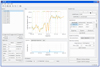 |
Fig. B.1. Main window of Redmost. |
 |
Fig. B.2. AAOmega spectrum of one galaxy from our sample (ID: MACS_2141, z∼0.33), with the redshift estimation performed using EZ. The spectrum has been smoothed with a Gaussian kernel with a sigma of 2 pixels. The key emission and absorption lines are marked with green lines. |
-
a line matching tool, that allows the redshift to be measured by manually selecting the lines on the spectra and matching their positions with a list of known ones;
-
a Redrock plugin that uses the functions and spectral templates provided by the Redrock python module, which is developed and maintained by the Dark Energy Spectroscopic Instrument (DESI, Flaugher & Bebek 2014) collaboration.
The Redrock plugin, in particular, allows Redrock to be run either on all the open spectra or just on a user-selected subset, and it automatically takes care to format the input data and retrieve the results. Since Redmost is built to be modular, following a plug-in style philosophy, redshift measurement functionalities can be easily extended and we will develop new plug-ins for other methods in future releases. The strength of this approach is that the redshifts can be measured independently by different methods and the results can be checked and validated directly on the spectrum plots, interactively, and within the sameprogram.
The spectroscopic redshift measurements can be exported either as a FITS table (or any other format supported by astropy) or as a Redmost project. The latter is a JSON file that contains in plain text all the information needed to restore the status of the application, beyond the measured redshifts. Redmost is in active development and the full documentation of the latest version, along with some tutorials, are available on the project home page: https://redmost.readthedocs.io.
Appendix C: Acknowledgements
We sincerely thank the anonymous referee for improving the overall quality of the paper. We greatly appreciate their time and effort in reviewing our work. RR, MDA, AM, ML and AI acknowledge financial support from INAF Large Grant 2022, FFO 1.05.01.86.16. ML and AI acknowledge financial contribution from the Italian Ministry grant Premiale MITIC 2017 and from INAF-Minigrant "4MOST- StePS: a Stellar Population Survey using 4MOST@VISTA" (2022). RR, MDA and AM acknowledge financial support through grants PRIN-MIUR 2020SKSTHZ, PRIN-MIUR 2017WSCC32 (PI: P. Rosati), INAF “main-stream” 1.05.01.86.20 (PI: M. Nonino)” and INAF “main-stream” 1.05.01.86.31 (PI: E. Vanzella). RR, MDA and AM acknowledge Balestra et al. (2016), Caminha et al. (2017) and the VLT programme IDs 186.A-0798, 094.A-0115(B), 094.A-0525(A). AG acknowledges the financial support of the MUR through the program “Dipartimenti di Eccellenza 2018-2022” (Grant SUPER-C).
All Tables
New catalogue of spectroscopic redshift of MACS0416 field obtained with AAOmega observations.
All Figures
|
Fig. 1. Imaging and redshifts spatial distribution for MACS0416. On the top left, the VST i-band image, covering a central region of the cluster (30′ × 30′), is shown with MUSE (red) and VIMOS (blue) redshifts, over the range z = [0.02 − 6.2]. The bottom left image shows the Hubble Frontier Fields (HFF) color image (2.8′), where MUSE yields additional z in the cluster core. The right color composite image combines VST g- and i- plus the VISTA Ks- bands. |
| In the text | |
|
Fig. 2. In the top panel is shown the spectrum of a galaxy from our AAOmega sample (ID: MACS64052446, z ∼ 0.40), with the z estimated via Redrock. The key emission and absorption lines are marked with coloured dashed lines (see legend at top). The variance of the spectrum is illustrated in the bottom panel. |
| In the text | |
|
Fig. 3. VST i-band image covering 1 deg2 (∼20 × 20 Mpc2), overlapped with the 1236 AAOmega measured redshifts (turquoise points). The light blue circles with black edges represent the new 148 members of MACS0416 from AAOmega catalogue, in the redshift range z = [0.382 − 0.412]. The region where VIMOS or MUSE redshifts are available over z = [0.02 − 6.2] range is represented as a blue rectangle. The black circle corresponds to the radial distance from the cluster centre of 5R200 ∼ 9.1 Mpc. |
| In the text | |
|
Fig. 4. Top left panel: Redshift distribution of the 1233 sources extracted from the AAOmega spectra. Three objects with redshift ≥1 were excluded from the plot for a better visualization of the distribution. Bottom left panel: Zoomed-in image of the redshift range of the members selected with AAOmega observations. Right panel: Redshift distribution of the 1017 from MUSE or VIMOS (blue) plus 148 from AAOmega (turquoise) spectroscopic cluster members selected in the range z = [0.382−0.412]. |
| In the text | |
|
Fig. 5. Average spectral properties of our sample as a function of colour and KKron as a proxy of the stellar mass. Left panel: Sample divided into red (72) and blue (76) galaxies, with their stacked spectra displayed in red and blue, respectively. A (g − r)Kron colour cut was used. The inset in the top left corner shows a colour distribution of our sample, where the x-axis represents the observed (g − r)Kron colour, corrected for extinction. Right panel: Whole sample divided into three subclasses based on the three bins of KKron. In red is the stacked spectrum of the brightest galaxies with KKron < 17.9 mag, in green that of the galaxies with intermediate luminosity 17.9 mag ≤ KKron < 18.9 mag, and in blue the stacked spectrum of the faint galaxies with KKron ≥ 18.9 mag. In the top left corner, an inset showing the trend between (g − r)Kron and KKron magnitude is reported. The dashed magenta line corresponds to the best fit of the linear correlation. In both panels, the stacked spectrum of the entire population of members (148) of MACS0416, obtained with AAOmega, is shown in black. All spectra are rest-frame and have been smoothed using a Gaussian kernel with a sigma of 2 pixels. The vertical dashed grey area corresponds to the spectral region of the join between the two arms. |
| In the text | |
|
Fig. 6. Left panel: Photometric density map of MACS0416 from Estrada et al. (2023), with all the new redshifts of objects with QF ≥ 2 (1236) obtained with AAOmega overlaid (white circles), highlighting the new spectroscopic cluster members (148) (light blue circles). Right panel: Same as left panel, with all the new spectroscopic cluster members (148) obtained with AAOmega overlaid, colour-coded as a function of δ. The red and green points are the members in the overdensities plus filamentary structures, while blue points are those in the underdense regions. |
| In the text | |
|
Fig. 7. Average spectral properties of our sample as a function of the local environment. Top panel: Stacked spectrum of the AAOmega members (148) is shown in black. The stacked spectra of galaxies located in overdense regions are shown in red; those in filamentary regions in green; and those in less dense areas, comparable to the field, in blue. All spectra are rest-frame and have been smoothed using a Gaussian kernel with a sigma of 2 pixels. The vertical dashed grey area corresponds to the spectral region of the join between the two arms. Bottom panels: (g − r)Kron (left) and KKron (right) distributions of the galaxies in our sample as a function of the same three δ bins (red, green, and blue). |
| In the text | |
|
Fig. 8. Average spectral properties of our sample of red and blue galaxies as a function of the local environment. Left panel: Stacked spectrum of the population of red members (72) of MACS0416, is shown in dark red, at the top of the image. The entire sample was then divided into three subclasses based on the three bins of density δ. The stacked spectra of the red galaxies located in overdense regions are shown in red; those in filamentary regions in coral; and those in less dense areas, comparable to the field, in orange. Right panel: Same as the left panel, for the blue members (76) of MACS0416. All spectra are rest-frame and have been smoothed using a Gaussian kernel with a sigma of 2 pixels. The vertical dashed grey area corresponds to the spectral region of the join between the two arms. We performed a Kolmogorov–Smirnov (KS) test on each pair of average spectra in the left and the right panels, obtaining p-values much smaller than 0.05 (effectively consistent with zero), which strongly supports our assumption that the average spectra of the different populations are statistically distinct. |
| In the text | |
|
Fig. B.1. Main window of Redmost. |
| In the text | |
|
Fig. B.2. AAOmega spectrum of one galaxy from our sample (ID: MACS_2141, z∼0.33), with the redshift estimation performed using EZ. The spectrum has been smoothed with a Gaussian kernel with a sigma of 2 pixels. The key emission and absorption lines are marked with green lines. |
| In the text | |
Current usage metrics show cumulative count of Article Views (full-text article views including HTML views, PDF and ePub downloads, according to the available data) and Abstracts Views on Vision4Press platform.
Data correspond to usage on the plateform after 2015. The current usage metrics is available 48-96 hours after online publication and is updated daily on week days.
Initial download of the metrics may take a while.