| Issue |
A&A
Volume 701, September 2025
|
|
|---|---|---|
| Article Number | A52 | |
| Number of page(s) | 12 | |
| Section | Stellar structure and evolution | |
| DOI | https://doi.org/10.1051/0004-6361/202555701 | |
| Published online | 03 September 2025 | |
Modeling the progenitors of low-mass post-accretion binaries
1
Goethe Universität Frankfurt Institut für Angewandte Physik, Max-von-Laue-Str. 1, 60438 Frankfurt am Main, Germany
2
Max Planck Institute für Astronomie, Königstuhl 17, 69117 Heidelberg, Germany
3
H.H. Wills Physics Laboratory, University of Bristol, Tyndall Avenue, Bristol, BS8 1TL
UK
⋆ Corresponding author: This email address is being protected from spambots. You need JavaScript enabled to view it.
Received:
28
May
2025
Accepted:
22
July
2025
Abstract
Context. About half of the mass of all heavy elements with mass number A > 90 is formed through the slow neutron capture process (s-process), occurring in evolved asymptotic giant branch (AGB) stars with masses of ∼1 − 6 M⊙. The s-process can be studied by modeling the evolution of barium (Ba), CH, and carbon-enhanced metal-poor (CEMP)-s stars.
Aims. Comparing observationally derived surface parameters and 1D local thermodynamic equilibrium (LTE) abundance patterns of s-process elements to theoretical binary accretion models, we aim to understand the formation of post-accretion systems. We explore the extent of dilution of the accreted material and describe the impact of convective mixing on the observed surface abundances.
Methods. We computed a new grid of 2691 stellar evolution models for low-mass post-accretion systems, including accretion from an AGB companion. A maximum-likelihood comparison to surface parameters and derived abundances determines the best fit models for a large observational sample of Ba, CH, and CEMP-s stars.
Results. We find consistent AGB donor masses in the mass range of 2 − 3 M⊙ across our sample of post-accretion stars. We find the formation scenario for weak Ba stars is an AGB star transferring a moderate amount of mass (≤0.5 M⊙) resulting in a ∼2.0 − 2.5 M⊙ Ba star. The strong Ba stars are best fit with lower final masses ∼1.0 − 2.0 M⊙ and significant accreted mass (≥0.5 M⊙). The CH and CEMP-s stars display lower final masses (∼1.0 M⊙) and small amounts of transferred material (∼0.1 M⊙).
Conclusions. We find that Ba stars generally accrete more material than CEMP-s and CH stars. We also find that strong Ba stars must accrete more than 0.50 M⊙ to explain their abundance patterns, and in this limit we are unable to reproduce the observed mass distribution of strong Ba stars. The mass distributions of the weak Ba stars, CEMP-s, and CH stars are well reproduced in our modeling.
Key words: accretion, accretion disks / nuclear reactions, nucleosynthesis, abundances / binaries: spectroscopic / stars: chemically peculiar / stars: low-mass
© The Authors 2025
 Open Access article, published by EDP Sciences, under the terms of the Creative Commons Attribution License (https://creativecommons.org/licenses/by/4.0), which permits unrestricted use, distribution, and reproduction in any medium, provided the original work is properly cited.
This article is published in open access under the Subscribe to Open model.
Open Access funding provided by Max Planck Society.
1. Introduction
Barium (Ba) stars, CH stars, and carbon-enhanced metal-poor (CEMP)-s stars are recognized as post-accretion binary systems showing enrichment in carbon and elements synthesized mostly through the s-process (Keenan 1942; Bidelman & Keenan 1951; Burbidge et al. 1957; Käppeler et al. 2011; Lugaro et al. 2023). Initially described as first ascent giants, the Ba, CH, and CEMP-s stars are not able to produce s-process material and self-enrich their envelopes. Additionally, dwarf stars have been observed carrying these signatures.
Discovered in the 1950s (Bidelman & Keenan 1951), Ba stars show enhancements in s-process elements. Detailed chemical abundance analyses have confirmed the s-rich nature of the Ba stars (Warner 1965; Allen & Barbuy 2006; Pereira et al. 2011; de Castro et al. 2016; Cseh et al. 2018; Karinkuzhi et al. 2018; Roriz et al. 2021a,b). The Ba stars’ characteristics include moderate to high metal content ([Fe/H] > −1.0), s-element enrichment, and mild carbon enrichment. The binary nature of these systems was recognized by McClure et al. (1980) and McClure (1984), and McClure & Woodsworth (1990) and Udry et al. (1998) later confirmed the link between the Ba stars and binary interactions with refined orbital parameters. More recent studies (Escorza et al. 2019; Jorissen et al. 2019) have contributed to the compilation of orbital properties and component parameters for increasingly large samples of Ba stars.
Keenan (1942) distinguished the CH stars from ordinary carbon stars by the strong CH molecular G-band near 4308 Å, and Bidelman & Keenan (1951) provided further classification based on their heavy element enrichment. Photometric surveys expanded the known population of CH stars, confirming their primary existence in the Galactic halo (Bond 1974). The CH stars share many properties with the Ba stars, but are found with higher carbon enhancements above [C/Fe] > + 0.5 and may be found at lower metallicities (−2.50< [Fe/H] < − 0.20). Recent studies (Goswami et al. 2006, 2016; Karinkuzhi & Goswami 2014, 2015; Purandardas et al. 2019) expand on the heavy element abundance patterns. McClure (1984) showed that CH stars exhibit long-term radial velocity variations, and show a very high binary fraction in the population. McClure & Woodsworth (1990) established that the CH stars have orbital properties consistent with mass transfer from an evolved asymptotic giant branch (AGB) companion with typically nearly circular orbits. The CH stars are a key population of stars, bridging the gap between the metal-rich Ba stars and the metal-poor CEMP-s stars.
The subclass of CEMP-s stars, identified by their enhanced surface abundances of s-process elements, were distinguished as a unique group among CEMP stars (Ryan et al. 1996; Norris et al. 1997). The CEMP-s stars reside at low metallicities ([Fe/H] < − 1.0, but often much lower, < − 2.0), have a high carbon-to-iron ratio ([C/Fe] > + 0.7), and have strong over-abundances of s-process elements such as barium ([Ba/Fe] > + 1.0). One of the most significant discoveries regarding CEMP-s stars is that nearly all of them are in binary systems, with a binary fraction near 100%, providing strong evidence of mass-transfer as the source of the chemical enrichment (Lucatello et al. 2005; Starkenburg et al. 2014; Hansen et al. 2016a). The binary nature of CEMP-s stars is widely supported by data acquired from extensive programs of radial velocity monitoring in which orbital periods range from hundreds to tens of thousands of days (Jorissen et al. 1998; Hansen et al. 2016a). With refined orbital parameters of the observed population, Izzard et al. (2010), Starkenburg et al. (2014), Hansen et al. (2016a,b), and Abate et al. (2018) show consistency with binary mass-transfer models. By studying the orbital properties of both CH and CEMP stars, Jorissen et al. (2016) found no discernible differences in the period-eccentricity distribution of the two groups. They remark that the two classes of stars should not be treated separately from the orbital perspective, but as one population. As similar post-mass-transfer systems at different metallicities, these three populations of stars provide valuable observational constraints on s-process nucleosynthesis models in AGB stars (Hansen et al. 2016a,b, 2019; Cseh et al. 2018, 2022).
The peculiar abundance patterns in these populations are understood to be the result of AGB mass-transfer in binary systems. To explain the origins of the chemical enhancements in these stars, various models of accretion and mass transfer have been developed with the aim of determining how AGB stars enrich their binary companions, the efficiency of accretion, and evolutionary links between classes of chemically peculiar stars. Boffin & Jorissen (1988) showed that for some Ba stars with short orbits, Roche-lobe overflow (RLOF) is a likely mechanism of mass transfer. However, many observed Ba, CH, and CEMP-s stars have long orbital periods where RLOF is not likely to occur.
In the Bondi-Hoyle-Lyttleton (BHL) accretion regime (Bondi & Hoyle 1944; Hurley et al. 2002; Edgar 2004) mass is captured from a stellar wind, where early models predicted inefficient accretion. Modern hydrodynamical simulations (Mohamed & Podsiadlowski 2007) show that wind Roche-lobe overflow (WRLOF) can significantly increase accretion efficiency, and can explain the enrichment observed in Ba, CH, and CEMP-s stars, even in wide binaries. Some models suggest that accreted material can form a circumstellar disk around the secondary, allowing for the retention of enriched material. Han et al. (1995) investigated the formation of Ba and CH stars via binary interactions, considering wind accretion, stable RLOF, and common-envelope evolution and ejection. Other modeling efforts in binary mass loss and accretion have been successful in generalizing the effects of interacting binaries (Karakas et al. 2000), but the amount of material transferred and the mass-transfer mechanism is generally poorly constrained for these post-accretion systems.
After material has been accreted, mixing processes within the accretor star will affect the observed surface abundances. Convective mixing becomes more important with the advance of the convective envelope as the star ascends the giant branch. Cristallo et al. (2011) showed that the third dredge-up is more efficient at lower metallicities, making overall s-process enrichment weaker in the metal-rich Ba stars. Other mixing processes have been explored by Matrozis & Stancliffe (2016), who showed how thermohaline mixing and dilution affect observed abundances in CEMP-s stars after accretion.
The nucleosynthetic s-process is expected to take place in the interiors of low- to intermediate-mass (1–6 M⊙) thermally pulsing AGB (TPAGB) stars (Gallino et al. 1998; Busso et al. 1999; Straniero et al. 2006; Karakas & Lattanzio 2014). In the framework of post-mass-transfer binaries, the more massive primary TPAGB star loses mass and pollutes the atmosphere of the less evolved companion (Roriz et al. 2024). At very low metallicities ([Fe/H] ≲ − 2.5), there are insufficient seed nuclei for the s-process to operate, and s-process enhancement from AGB stars is not expected at such metallicities (Hansen et al. 2014; Lombardo et al. 2025). Karakas & Lattanzio (2014) modeled yields of s-process elements in AGB stars and showed that low-mass (1–3 M⊙) AGB stars are primarily responsible for the chemical signatures observed in these post-mass-transfer systems. The FUll-Network Repository of Updated Isotopic Tables & Yields (FRUITY) models (Straniero et al. 2006; Domínguez et al. 2011; Cristallo et al. 2015) provide updated s-process element yields from AGB stars at different masses and metallicities, making them useful for predicting s-process abundance patterns in Ba, CH, and CEMP-s stars, determining neutron source efficiency, and comparing observed stellar abundances to theoretical yields.
The mass distribution of Ba stars was studied by Escorza et al. (2017) and is described by two Gaussians with a main peak at 2.5 M⊙ with a standard deviation of 0.18 M⊙, and a broader tail at higher masses (up to 4.5 M⊙), which peaks at 3 M⊙ with a standard deviation of 1 M⊙. A complementary study in Jorissen et al. (2019) found a similar distribution of masses with compatible metallicities for Ba stars. Post-accretion binaries play a crucial role in stellar population synthesis and binary population synthesis modeling.
The observable surface abundances of these stars are strongly dependent on the amount of mass transferred, ΔM, when the mass is transferred during the evolution of the secondary, and the mixing processes within the accretor star. One of the outstanding questions is how much material is actually accreted by the companion, which provides a direct link to the efficiencies of AGB mass transfer. Stancliffe (2021) has modeled Ba star progenitor systems at a fixed metallicity of [Fe/H]} = −0.25 and a fixed post-accretion Ba star mass of 2.5 M⊙, corresponding to the average mass of Ba giants determined by Escorza et al. (2017). Under these assumptions, Stancliffe (2021) found that the amount of accretion in Ba star systems is typically small, on the order of 0.10 M⊙.
Our grid of stellar evolution models spans a wider range in mass and metallicity, compatible with metal-poor CEMP-s and CH stars and metal-rich Ba stars. Such models give us an insight into the progenitor system, including the mass of the primary AGB star, how much material is transferred, and the initial mass of the observed polluted star. We compare observationally derived stellar surface parameters and abundances to our evolution models. When viewed together as multiple populations formed through similar scenarios, these systems trace the formation processes of heavy elements produced in AGB stars and accretion in low-mass binary systems. We comment on the orbital properties of these populations in the literature.
2. Observational data
We compared our models to stellar parameters and 1D local thermodynamic equilibrium (LTE) surface abundances derived from high-resolution (30 000 < R < 60 000) spectroscopic observations. We included the homogeneously analyzed sample of Ba, CH, and CEMP-s stars from Dimoff et al. (2024). We collected further data from the large sample of strong- and weak Ba stars from de Castro et al. (2016), supplemented by additional heavy element abundances from Roriz et al. (2021b). We expanded our analysis to the metal-poor regime and included CH and CEMP-s stars from Goswami et al. (2006, 2016, 2021), Karinkuzhi & Goswami (2014), Karinkuzhi & Goswami (2015). For each of our observational samples, we collected stellar surface parameters Teff, log g, and [Fe/H] (see Figure 1) and surface abundances of C and heavy elements produced via the s-process, as well as the r-process tracer Eu. Not all of the observational datasets contain the same derived elemental abundances. In some cases, the observable Ba lines are saturated and not used for abundance derivations. By comparing our models to different populations of stars believed to have accreted material from a previous AGB companion, we are able to make predictions about AGB masses, stellar masses, and accretion masses, and make distinctions between metal-poor and metal-rich populations. These observational data are non-homogeneous and do not contain the same elemental abundances, as we draw our observed data from different sources.
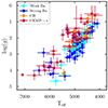 |
Fig. 1. Kiel diagram showing surface gravities and effective temperatures for the collected observational sample. Blue data points are strong Ba stars, cyan data points are weak Ba stars, orange data points are CH stars, and red data points are CEMP-s stars. Surface parameters and abundances are collected from Dimoff et al. (2024), de Castro et al. (2016), Roriz et al. (2021a), Goswami et al. (2006, 2016, 2021), Karinkuzhi & Goswami (2014, 2015). |
We took note of stellar labels from the literature, and we applied corresponding labels based on metallicity and chemical enrichment. The original CEMP classification scheme from Beers & Christlieb (2005) and Masseron et al. (2010) defines metal poor stars as those with [Fe/H] < −1.00. Within this category, we define CEMP stars in our sample as stars with [C/Fe] > 0.70. To further classify the stars in our sample, we defined [ls/Fe] as the average abundances of Sr, Y, Zr, and Mo with respect to Fe, and [hs/Fe] as the average abundances of Ba, La, Ce, Pr, Nd with respect to Fe. From Bisterzo et al. (2014) Nb is mostly produced by the s-process, but Nb abundances in the de Castro et al. (2016) dataset are systematically higher than the models, and we exclude Nb from the computation of [ls/Fe].
Following Hansen et al. (2019), we classified our CEMP population based on relative ratios of light- and heavy- s-process element abundances. We substituted [ls/Fe] for [Sr/Fe] and [hs/Fe] for [Ba/Fe] to account for observations where derivations of these elements are missing. If the CEMP star has enhancements in both light and heavy s-elements ([Sr/Fe] or [ls/Fe] > 0.30 and [Ba/Fe] or [hs/Fe] > 0.30) and does not have significant r-process enhancements ([Eu/Fe] < 0.50), it is a CEMP-s star. Otherwise, we excluded any -r/s enriched stars from our investigation. The CH stars also have high carbon enhancements [C/Fe] > 0.70, and are expected to have enhancements in s-process material with [ls/Fe] > 0.30 or [hs/Fe] > 0.30, but may have metallicities up to [Fe/H] < −0.20. If there are no enhancements in either r- or s-process elements, the star is labeled as a CEMP-no star. In our accretion modeling, we omit the CEMP-r, -r/s, and -no stars, as they are not believed to have accreted pure s-process signatures from a former AGB companion.
The Ba stars have higher metallicities ([Fe/H] > −1.00) and are generally not as enhanced in carbon as the CEMP and CH populations. Ba stars are split into two categories: strong- and weak Ba stars. Karinkuzhi et al. (2021) provides a classification of the Ba stars based on heavy element abundance ratios. We use the [ls/Fe] and [hs/Fe] ratios to satisfy the criterion that more than three elements in the light- and heavy- s-process peaks are included. A star is a “Ba-no” star if both [hs/Fe] and [ls/Fe] < 0.20. A “mild” (or “weak”) Ba star has either [hs/Fe] or [ls/Fe] in the range ![Mathematical equation: $ 0.20 < \rm{[hs/Fe]}\; or\; \rm{[ls/Fe]} < 0.80 $](/articles/aa/full_html/2025/09/aa55701-25/aa55701-25-eq1.gif) , and a “strong” Ba star has either [hs/Fe]} or [ls/Fe] > 0.80. Our observational sample is displayed in Figure 1, where the stars are colored following these classification schemes.
, and a “strong” Ba star has either [hs/Fe]} or [ls/Fe] > 0.80. Our observational sample is displayed in Figure 1, where the stars are colored following these classification schemes.
Some of our observational datasets contain alpha elements, including Mg. We find observed Mg abundances consistently higher than the AGB yield predictions, and the inclusion of Mg and other alpha elements is a hindrance in finding the best fit model, decreasing the likelihood that any given model fits the observed data. Previous studies on Galactic chemical evolution have also observed problems where the observations of Mg are systematically higher than the model predictions Romano et al. (2010), Prantzos et al. (2018), Jost et al. (2025). With this justification, we omitted Mg and other alpha elements in the fitting routine, and focused only on C and the s-process material that is produced in the companion AGB star.
When explicitly stated, or when the uncertainties are not provided in the source material, we treat abundance upper limits by taking the value of the abundance to be consistent with zero (0), and the observed “upper limit” is taken as the 2σ uncertainty. In this sense, the true uncertainty in the abundance is one half of value of the upper limit.
3. Modeling methods
We computed a grid of stellar evolution models using the STARS code (Eggleton 1971, 1972; Pols et al. 1995; Stancliffe & Eldridge 2009), including the addition of mass to simulate binary accretion. The program solves the equations of stellar structure with the chemical evolution of seven energetically important species: 1H, 3He, 4He, 12C, 14N, 16O, and 20Ne. At the convergence of every time step in the model, a network of 40 isotopes was computed (Stancliffe 2005). Our models use 499 mesh-points, no additional mass-loss, a mixing length parameter of α = 2.025 following Stancliffe (2021), and a prescription for convective overshoot following Schroder et al. (1997), using δov = 0.15 from Stancliffe et al. (2015). We defined the primary star as the AGB donor star, and the secondary star as the accreting Ba, CH, or CEMP-s star.
In our models, the main mixing processes occur due to convection as the accretor star ascends the giant branch. We do not consider thermohaline mixing, and note that thermohaline mixing has been shown to be an effective means of changing the surface composition of low-mass stars on the upper part of the giant branch (Stancliffe 2015). While Stancliffe et al. (2007) found that thermohaline mixing can be effective on the main sequence, a follow-up study (Stancliffe & Glebbeek 2008) found that the effects of gravitational settling can inhibit thermohaline mixing at low metallicities and, in cases where a small quantity of material is accreted, can be suppressed almost completely. Stancliffe (2021) showed that thermohaline mixing plays an overall less significant role in diluting surface abundances compared to the convective mixing upon first dredge-up (FDU) in metal-rich stars.
The grid of stellar evolutionary tracks is parameterized by the metallicity, the AGB donor mass, the initial mass, and the amount of accreted material. Metallicities range from Z = 0.0001 ([Fe/H] = − 2.15) to Z = 0.010 ([Fe/H] = − 0.15), complementary to the set of barium star models from Stancliffe (2021) who computed models for metallicity of [Fe/H] = − 0.25. It is assumed that the AGB donor and companion are the same metallicity. Our models cover a post-accretion final mass range to include low- and intermediate-mass stars with final masses from 0.80 to 5.0 M⊙. The initial masses of the models were determined by subtracting the prescribed amount of accreted material. For any given final mass, initial masses range from Mf − 0.50 M⊙ to Mf − 0.05 M⊙, with accretion masses equal to 0.05, 0.10, 0.20, 0.30, 0.40, and 0.50 M⊙. In total, we generated 2691 stellar evolution models. Following Stancliffe (2021), each stellar model was evolved up to an age determined by the lifetime of the AGB companion, where material from the AGB was added to the stellar surface at a constant rate until the final target mass was achieved. The composition of the AGB ejecta was taken from the FRUITY database Domínguez et al. (2011), Cristallo et al. (2011, 2015). The FRUITY database contains around 120 models that range in initial mass from 1.3–6 M⊙ and metallicities from Z = 0.0001 ([Fe/H] = − 2.15) to 0.03 ([Fe/H] = + 0.32).
After the accretion phase has ended, the secondary star continues to evolve, taking the new surface composition into account. Surface abundances are diluted following mixing processes in the accretor star. We used a tracer element “arbitrarium” to define how the AGB material is mixed into the secondary star. If the material originated from the AGB star, the value of arbitrarium was set to one, and it was set to zero if it originated within the secondary. We quantified the mixing following
 (1)
(1)
where Xactual is the surface abundance, i is the timestep, Xarb is the value of arbitrarium, Xacc is the ejecta abundance, and Xoriginal is the elemental abundance in a star of solar metallicity, taken from Asplund et al. (2009), scaled by the metallicity of the star. The effects of mixing due to convection become more prominent with lower surface gravities and the inward advance of the convective envelope as the star ascends the giant branch.
The time of accretion changes with the mass and metallicity of the AGB donor star, with more massive and more metal-rich AGBs donating their material earlier than lower mass and more metal-poor stars. To this end, we first ran the STARS code for single stars with masses of 1.3, 1.5, 2.0, 2.5, 3.0, 4.0, and 5.0 M⊙, compatible with the AGB masses in the FRUITY database. Evolution in the STARS code continues past the core helium burning phase and begins the ascent of the AGB, beyond the evolutionary states of the observed stars.
A selection of evolutionary tracks from our grid of models can be seen in Figure 2, where in the left panel the evolutionary tracks are offset from one another in the Kiel diagram. The accretion phase is highlighted in blue, where for the lowest initial mass tracks there is a noticeable change in temperature between the beginning and end of the accretion phase. The right panel of Figure 2 shows the surface abundance of [Ba/Fe], an element produced in AGB stars, as a function of log(Age/yr). Our models are parameterized such that after the star accretes the specified amount of mass, the surface abundances are changed to reflect that of the transferred AGB material. Beyond this, the convective envelope mixes and dilutes the surface abundances.
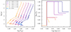 |
Fig. 2. Left: Evolutionary tracks for a sample of stars with mfinal = 2.50 M⊙ at [Fe/H] = −0.15 with varying initial masses and accretion masses, with accretion phases for each model highlighted in blue. Right: Relative surface abundance of the s-process element Ba with log10(Age/yr). The abundance is elevated after the accretion phase, and after the onset of first dredge-up the surface abundance is diluted. |
An example Kippenhahn diagram is shown in Figure 3. In this example, we display the structure of a 2.0 M⊙ star accreting 0.5 M⊙ of material from a 2.5 M⊙ AGB primary. The total mass is plotted against the model number, a proxy for time. The logarithm of the stellar age in years is included on the upper x axis. The purple and green regions denote radiative and convective zones, respectively, determined by computing the difference between the radiative and adiabatic transfer gradients, shown in the color bar. The onset of FDU is visible in the advance of the convective envelope toward the core as the star ascends the giant branch around model number 4500, as well as the onset of core He burning as the star begins to ascend the AGB around model number 5250. The accretion phase is shown as an increase in the overall mass of the star. In this case, accretion occurs while the secondary star is on the main sequence.
We describe the general features of our grid of models by focusing on the case of a 2.00 M⊙ star accreting 0.5 M⊙ from a 2.50 M⊙ AGB star at a metallicity of [Fe/H] = − 0.15 (seen in Figure 3), which starts to transfer mass at a stellar age of around 780 Myr. At this point, the 2.00 M⊙ star reaches a core helium abundance of XHe ∼ 0.48, and the convective core contains around 0.64 M⊙ of material. As accretion progresses, the convective core expands to reach a mass coordinate around 0.77 M⊙, where the core helium abundance is reduced as fresh hydrogen is ingested into the core of the now more-massive star. Since we are only accounting for mixing due to convection, the accreted layer remains on the stellar surface until the onset of FDU as the star ascends the giant branch. At its maximum depth, the convective envelope reaches a mass coordinate of around 0.50 M⊙, and penetrates the outer layers of the core. This signifies the maximum dilution of the accreted material, as the envelope will not reach this depth for the remainder of the lifetime of the star. As in Stancliffe (2021), we can define the dilution factor
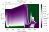 |
Fig. 3. Example Kippenhahn diagram for a 2.00 M⊙ star accreting 0.50 M⊙ of material from a 2.50 M⊙ AGB star at a metallicity of [Fe/H] = − 0.15. Green colors denote convective regions, and purple colors denote radiative regions, determined by the computed difference in the radiative and adiabatic transfer gradients. In the total mass on the y axis, the accretion phase can be identified by the increase in mass. The upper x axis shows log10(Age/yr), and the lower x axis shows the model number, which is highly nonlinear with respect to time. |
 (2)
(2)
where Macc is the mass of the accreted material and Mmix is the mass through which it is mixed. At this point, d = 0.25. While expressed in different notation, this is analogous to the dilution factor described in den Hartogh et al. (2023).
As the initial mass ratio, q, of the binary approaches one, the accretion happens later in the evolution of the secondary star (see Figure 2). A secondary star with an initial mass of 2.40 M⊙ accretes after it has left the main sequence and is going through the core-He burning phase, shown in the orange evolutionary track in Figure 2. At this point, the convective envelope is considerably shallower than at the onset of FDU, and has a thickness of only about 0.70 M⊙. Convection quickly dilutes the accreted material and, as the star ascends the AGB, the accreted material is diluted further by the second advance of the convective envelope. During this time, the maximum mass contained in the envelope is ∼1.90 M⊙.
The evolution of the surface abundances generally follows that of the dilution factor as temperatures in the envelope are not high enough to process the heavy elements accreted from the AGB star. In the right panel of Figure 2, the surface abundances of the s-process element [Ba/Fe] are displayed. With only convection acting, the abundance of Ba is unchanged from the end of the accretion phase until the onset of FDU. With the inward advance of the convective envelope, the accreted material is mixed and diluted within the stellar interior and the surface abundance falls dramatically. With the increase in the mass of the accretor star, the mass of the convective envelope increases, and through this the surface abundances are diluted more effectively.
4. Results
4.1. Comparison to the models
When comparing to our observational sample, we consider models in the grid that have mass ratios q = M2/M1 ≤ 1.00. Otherwise, the companion would be more massive than the AGB star and will have evolved first. We require that each observed star have measured surface parameters Teff, log(g), and [Fe/H]}, and computed 1D-LTE abundances for at least one s-process element in each s-process peak. Many evolutionary tracks exist on the HR diagram during periods of rapid evolution (i.e., the red giant branch (RGB), where many stars in our sample lie), and the density of model data points in these regions can be preventative in selecting a model that is physically representative of the observed system. Since this is the case, we exercise caution when addressing the best fit models using this method.
To quantify the comparison between our models and observations, we computed the likelihood for each model at each time step, comparing the observed values of the stellar surface temperature, surface gravity, metallicity, and available abundances to those within the models. To find the best fit model, we maximized the likelihood function by minimizing the χ2 difference between the models and observations. One caveat to the χ2 method is that it generally assumes the parameters being fit are uncorrelated; in our comparison, this is not true. The relative abundances of heavy elements are highly correlated with one another as well as the surface parameters. In many cases, the difference in χ2 between best-fit models can be small, indicating only subtle differences between them.
4.2. Fits to known Ba, CH, and CEMP-s stars
We compare our model grid to the properties of known Ba, CH and CEMP-s stars. Comparing the effective temperature, surface gravity, metallicity, stellar mass, and elemental abundance patterns, we determine the most probable initial configuration to have produced the observations. We estimate the mass of the AGB star that transferred mass to the observed star, the initial and final mass of the chemically peculiar star, and the amount of accreted material required to reproduce the observed chemical signatures. We are able to recover the metallicity of the observed system with high accuracy. For each star, we visually examine the three best fit models according to their χ2 values. In many cases, there is only a small difference in χ2 between the best fit models. Before discussing the sample as a whole and the constituent populations of stars within our sample, we describe individual objects. Stancliffe (2021) analyzed a subset of 74 Ba stars from de Castro et al. (2016), although with fewer abundances compared to our inclusion of the data from Roriz et al. (2021a). Here we examine our own fits to some stars examined by Stancliffe (2021).
4.2.1. PV UMa
We find a very good fit for this weak Ba star in both the Kiel diagram and in abundance space, shown in the top panels of Figure 4. Our best fit to this star is a 2.40 M⊙ star accreting 0.10 M⊙ of material from a 2.50 M⊙ AGB star at a metallicity of [Fe/H] = − 0.37. The observed temperature The two best fit models could each be likely scenarios to produce this and other weak Ba star systems. Recently observed and studied by Dimoff et al. (2024), PV UMa is best fit on the second ascent of the giant branch, after the onset of core He burning. Computed abundances including carbon are well represented in the models, except for a over-abundance of Sr and an under-abundance of Ce. The low accretion mass and significant mixing on the giant branch results in relatively low surface abundances compared to the Ba strong stars
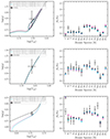 |
Fig. 4. Kiel diagrams and abundance fits for the weak Ba star PV UMa, the strong Ba star HD 123949, and the CEMP-s star CS 29512-073, each showing the three best-fitting models and their associated χ2 values. |
4.2.2. HD 123949
This object is representative of a large portion of the strong Ba stars in the de Castro et al. (2016) sample in both the Kiel diagram and in abundance space. An acceptable fit is obtained for this system, shown in the middle panels of Figure 4. This star lies directly on the evolutionary track for a 0.95 M⊙ star and the abundances are well fit, save for slight over-abundances in Nb and Nd. The low χ2 values indicate a good fit, given the number of fitting parameters. We find best fit models to be low initial mass secondary stars Mi ∼ 0.45 − 0.55 M⊙, accreting significant (> 0.40 M⊙) amounts of material from a 2.50 M⊙ AGB star resulting in a 0.95 M⊙ Ba giant. This does not fully agree with estimated Ba star masses from Escorza et al. (2017). More massive stars will have more massive convective envelopes, which will more efficiently mix and dilute surface abundances on the ascent of the giant branch, and a less massive accretor star will retain higher surface abundances. However, it may be an outlier in the strong Ba star mass distribution.
4.2.3. CS 29512-073
In this CEMP-s star, we find an excellent match in metallicity with both observed and modeled [Fe/H] = − 2.15. The precise observed stellar parameters are in good agreement with low-mass stellar evolution tracks on the subgiant branch, with best fit final masses between  M⊙. These values are in good agreement with theoretical masses of metal-poor stars. Carbon is over produced by the models compared to the observations; thermohaline mixing on the main sequence could dilute the surface abundance of C. Abundances of heavy elements are generally fit by our modeling aside from a slight overabundance in Nd and an overabundance in Sm past the second s-process peak. The best fit AGB mass is 2.50 M⊙, and our modeling suggests around 0.20 M⊙ of material accreted from the former AGB companion.
We present histograms of model parameters for our complete sample in Figure 5. The weak Ba stars are shown in cyan, the strong Ba stars in blue, the CEMP-s stars in red, and the CH stars in orange. While our grid is not continuously nor equally spaced in initial nor final mass, we are able to make generalized statements about the progenitors of these post-accretion systems. We recover the metallicity distribution of stars in our sample, and since our model grid is limited to metallicities above [Fe/H] = − 2.15, we make a cut on the observed stars at [Fe/H] > − 3.00.
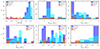 |
Fig. 5. Histograms of model parameters for the different classes of stars in our investigation. Dark blue regions are strong Ba stars, cyan regions are weak Ba stars, red regions are CEMP-s stars, and orange regions are CH stars. |
Overall, there is a clear preference of donor AGB masses across all stellar classifications with a very strong peak with a mean of ⟨MAGB⟩ = 2.70 M⊙. This is expected, as the s-process production rates peak in this mass range. Fits to the strong Ba stars show a very pronounced peak at an AGB mass of 2.50 M⊙, with a width of σ = 0.52 M⊙. For the weak Ba stars, most of the fits suggest an average AGB mass of ⟨MAGB⟩ = 2.80 M⊙. The distribution is broader compared to the strong Ba stars, with a width of σ = 0.78 M⊙. For both the carbon-enhanced CH and metal-poor CEMP-s populations, the preferred AGB mass is ⟨MAGB⟩ = 2.80 M⊙ with an even broader distribution (σ = 0.88).
Across the four different populations of post-accretion systems analyzed, all display non-Gaussian behavior in their initial and final mass distributions. The weak Ba stars show a broad distribution in initial mass ⟨Minit⟩= 1.70 M⊙ with a width of σMinit = 0.74, and final masses around ⟨Mfinal⟩ = 2.30 M⊙, and σMfinal = 0.75. The mass ratios of the weak Ba stars show a peak at higher values close to q = 0.90 with a tail down to low mass ratios of q = 0.10. The models suggest that weak Ba stars accrete moderate amounts of material; on average, they accrete about 0.35 M⊙ from their AGB companion.
In the strong Ba stars, we find a very dominant peak at low initial masses around 0.5 M⊙ with a tail extending up to 2.50 M⊙. The final masses are concentrated at about 1.00 M⊙ with a tail extending as high as 3.00 M⊙. The mass ratios of strong Ba stars is almost opposite that of the weak Ba stars, with most models fitting low q values of 0.20. There is a long tail extending to higher mass ratios, with a small peak at mass ratios close to q = 1.0. The models suggest that for strong Ba stars, large amounts of material have been accreted, with most fits showing 0.50 M⊙. The distribution is strongly peaked at high accretion masses, with few systems indicating smaller amounts of accretion. This is more material compared to the weak Ba stars, which is reflected in the observed higher surface abundances in the strong Ba stars.
At intermediate metallicities, the CH stars show initial masses with peaks at ≈0.50 M⊙ and a small broader peak at ≈2.00 M⊙. Final masses show corresponding peaks at ≈0.90 M⊙ and around 2.10 M⊙. Mass ratios in the CH stars are distributed between low (≈0.20) and high (≈0.98) values. The distribution of accretion masses in the CH systems display no clear preference in accretion masses. The number of CH stars in our sample is likely too low to make strong claims about the population as a whole.
At the lowest metallicities, the CEMP-s stars are somewhat scattered in initial and final masses. The majority of initial masses show peaks at ≈0.50 M⊙ and ≈2.0 M⊙ with a tail extending to higher initial masses. Most of the final masses show a peak around 0.90 M⊙, with a second peak close to 2.70 M⊙. As in the initial masses, there is a tail extending to higher masses. This could be dwarf stars in our sample, which are not as well modeled as the giant stars due to less intense convective mixing, or giant stars with very low surface gravities with values log(g)≲0.5 and very high derived abundances [ls/Fe] or [hs/Fe] ≳1.50. Initial mass ratios for the metal-poor systems show two clear peaks at q ≈ 0.30 and q ≈ 1.00, with a preference for higher initial mass ratios. Our modeling finds low accretion masses around 0.05 M⊙ for the CEMP-s stars.
5. Discussion
The strong Ba stars almost always accrete the maximum amount of mass, and the final mass distribution we recover does not fully agree with that of Escorza et al. (2017), where we find lower initial and final masses for many strong Ba stars by about a full solar mass. At higher masses, the more massive convective envelope dilutes surface abundances more efficiently compared to lower masses, and to maintain the observed higher surface abundances in the strong Ba stars, lower masses are required. We note our sample of Ba stars is only from de Castro et al. (2016) and Dimoff et al. (2024), where the larger Escorza et al. (2017) sample includes the de Castro et al. (2016) dataset, plus more Ba stars compiled from Lu et al. (1983), Lu (1991), Edvardsson et al. (1993), Bartkevicius (1996). The differences in average mass could be influenced by the larger sample.
We find that when accretion happens while the secondary is on the first ascent of the giant branch, the mixing processes within the advancing convective region have a significant effect in quickly diluting the surface abundances. Our models generally suggest higher accretion masses in secondary stars accreting on the main sequence or while first ascending the giant branch, compared to those close to the tip of the RGB, or near the onset of core He burning. This is also for evolutionary reasons, where in systems with mass ratios q ≈ 1 the primary and secondary stars are of near equal mass and can evolve nearly simultaneously.
Comparing our models and the observational data, we find a similar effect in the relative abundance uncertainties as the number of available abundances themselves. The average uncertainty in the Dimoff et al. (2024) abundances is σ[X/Fe] ∼ 0.15, where in the combined de Castro et al. (2016) and Roriz et al. (2021a) dataset it is σ[X/Fe] ∼ 0.20, and we find consistently smaller uncertainties approximately equally important when one has fewer computed abundances. The combined dataset from Cristallo et al. (2016) (and references therein) has average abundance uncertainties of σ[X/Fe] ∼ 0.23, and the CEMP-s stars dataset from Goswami et al. (2021) reports uncertainties of σ[X/Fe] ∼ 0.25, on average.
In the evolution of low-mass metal-poor stars, we generally find the accretion happens while the secondary star is on the main sequence. With initial AGB masses much higher than accretor masses (2.50 M⊙ vs. < 1.00 M⊙), the secondary star is on the main sequence when the AGB star begins thermal pulsations. Without thermohaline mixing, the surface abundances remain nearly constant until the onset of first dredge-up, making the differentiation between best fit models in this regime difficult (Stancliffe et al. 2007; Stancliffe & Glebbeek 2008). Thus we find this set of models better for analyzing giant stars, and main sequence stars may not be as representative.
We find it unlikely that all barium stars are observed shortly after the accretion process has ended, as would need to be the case for initial mass ratios very close to q = 1, where mixing on the giant branch is very effective and quickly dilutes surface abundances (see the right panel in Figure 2). Thus, larger accretion masses at lower initial mass ratios make sense for stars that exhibit large surface abundances of heavy elements. As the secondary star gains mass, it will alter its evolutionary path to follow that of the post-accretion mass. Some models in the grid have initial mass ratios of q > 1.0 where the secondary star is more massive than and would evolve more quickly than the primary. While these models could provide useful in analyzing systems with multiple mass transfer events, we do not consider these models in this analysis.
A few stars in our sample are poorly fit due to relatively low surface gravities (log(g)≤0.50), very high surface abundances of heavy elements where [ls/Fe] or [hs/Fe] ≳ 2.00, large amounts of Eu compared to the s-process elements, or some combination of these. For a few observed systems, only one derived elemental abundance exists in each of the first two s-process peaks, providing only weak constraints in the fitting routine. Very few evolutionary tracks with high elemental abundances extend toward the upper part of the AGB phase in the Kiel diagram, and the ones that do result in high masses close to 5.00 M⊙ that do not agree with the theoretical masses of stars in our observational sample. These also correspond to AGB masses of 5.00 M⊙ by the construction that the AGB mass must be larger than the initial mass of the observed star. Large χ2 values on the order of ≳70 indicate poor fits in these instances. Fits resulting in high masses often find flattened abundance patterns indicating the accreted material has been fully diluted, and the surface abundances have returned to the un-enhanced values.
5.1. Mixing and dilution
Matrozis & Stancliffe (2016) found that atomic diffusion does not have a substantial effect on the surface abundances of CEMP-s stars, so the dilution of the accreted material, while variable in degree from one star to the next, is most likely the same for all elements, and the mass ratios and overall pattern will be preserved. Thermohaline mixing on the main sequence will dilute the surface abundances to some extent. Stancliffe (2021) tested the inclusion and exclusion of thermohaline mixing in stars, and after the onset of FDU the surface abundance ratios of heavy elements between the two cases are nearly identical in Ba stars. Convective mixing processes in giant stars outweighs thermohaline mixing at higher metallicities, and the overall level of mixing in both scenarios is the same after FDU. In more metal-poor stars, this is not the case; Stancliffe et al. (2007) found that thermohaline mixing is on the main sequence is effective for light elements C, N, and O, and predicts different surfaces abundances for the CEMP-s stars compared to models with purely convective mixing. Including additional mixing processes, Stancliffe & Glebbeek (2008) found that the effects of gravitational settling can inhibit thermohaline mixing in CEMP-s stars and, in cases where a small quantity of material is accreted, mixing can be suppressed almost entirely.
The accretion phase in our models coincides with the AGB phase of the donor, so the initial mass ratio of the system effectively controls when the accretion phase will happen during the lifetime of the secondary. If accretion occurs while the secondary is on the main sequence or on the subgiant branch, the onset of first dredge-up (FDU) will severely deplete the surface abundances. If accretion happens after the onset of FDU, significant mixing will still occur in the convective envelope. Matrozis et al. (2017) suggests that in the wind regime only about 0.05 M⊙ of material can be added to the accreting star before it reaches critical rotation, which we find is able to explain the chemical enrichment of many CEMP-s stars, but not the Ba stars which require more mass to be accreted. According to Matrozis et al. (2017), the specific angular momentum of the accreted material should be be lower than the Keplerian value by about an order of magnitude, or significant angular momentum losses must occur for substantial accretion to take place. This may not be a significant issue for the weak-Ba stars, where the larger radius of the giant accretor star requires more angular momentum transfer to reach the critical rotation velocity, allowing more mass to be accreted. For the strong-Ba stars, which tend to accrete significant amounts of material on the main sequence, this poses a problem, and BHL wind mass transfer is not applicable to these systems.
5.2. Accretion efficiencies
For our binary systems, we computed the accretion efficiency, ηacc, by dividing the amount of mass gained by the accretor by the total mass lost by the AGB star in the system:
![Mathematical equation: $$ \begin{aligned} \eta _{\rm acc} = (m_{\rm final} - m_{\rm initial}) / (m_{\rm AGB} - m_{\rm WD}) \times 100\;[\%]. \end{aligned} $$](/articles/aa/full_html/2025/09/aa55701-25/aa55701-25-eq5.gif) (3)
(3)
In this sense, we assume nonconservative mass transfer. We estimate white dwarf masses using tabulated H-exhausted core masses from Cristallo et al. (2015) for the given AGB mass and metallicity of the model. We compare the white dwarf masses from the FRUITY models used in this study to the computed dynamical estimates from Dimoff et al. (2024) and find good agreement. Additionally, we find no significant differences between our samples of CH and CEMP-s stars in this analysis of accretion efficiencies and in this instance we treat them as one metal-poor and carbon-rich population, in agreement with Jorissen et al. (2016). We note that this could be due to the relatively low number of CH stars studied.
We compare our computed ηacc to 3D hydrodynamical wind mass-transfer models from Liu et al. (2017) in Figure 6, where the dashed and dotted black lines are linear and fifth-order polynomial fits from the 3D models, respectively. These simulations generally result in low accretion efficiencies, with a trend toward higher efficiencies at higher mass ratios.
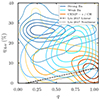 |
Fig. 6. Computed accretion efficiencies for our sample populations. Purple-blue contours are the strong Ba stars, and the green contours are the weak Ba stars. Red-yellow contours are our carbon-enhanced sample, including both CH and CEMP-s stars. |
The models in our grid are discrete points, and many times the same model is chosen to represent multiple modeled systems. For this reason, we present our populations as contours in η − q space. We see a general trend of increasing efficiency, η, with decreasing mass ratio, q, across the different stellar populations. The metal-poor stars require less accretion in systems with initial mass ratios closer to q = 1 to reproduce the observed surface abundances, resulting in lower efficiencies. The bimodal distribution of the carbon-enhanced systems is well shown in the density contours. At lower mass ratios below about q ≲ 0.5, there are only a few carbon-enriched systems with relatively low mass-transfer efficiencies, ≈10%. Higher-metallicity systems with lower mass ratios congregate in efficiencies around ∼25%; these are the strong Ba stars. Generally, we find that accretion masses greater than about 0.30 M⊙ will result in efficiencies higher than the theoretical wind mass transfer regime described in Liu et al. (2017).
5.3. Possible mass transfer scenarios
The mechanism of mass transfer in AGB stars is directly linked to the properties of the initial binary orbit and the relative velocity of the AGB wind compared to the orbital velocity. There are multiple regimes in which mass transfer can occur, and in all of them some amount of angular momentum transfer will perturb the orbit. The resulting orbit will likely not be the same as the initial orbit of the binary.
Krynski et al. (2025) suggest that WRLOF and non-conservative mass-transfer with the presence of a circumbinary disk provides mechanisms for both high accretion efficiencies and enhanced eccentricities, explaining the observed orbital geometries of these post-accretion systems. For slow and dense stellar winds with low wind velocities compared to the orbital velocity, structures resembling wind Roche-lobe overflow form as the stars approach periastron, indicating a form of tidally enhanced mass transfer (Mohamed & Podsiadlowski 2007, 2012). Through this process, the circumstellar outflows are nonspherical and concentrated in the orbital plane of the binary. The non symmetric flows contribute to maintaining or increasing the eccentricity of the binary system. Abate et al. (2013) discusses wind-RLOF in the context of binary population synthesis for the CEMP-s stars, finding that, pending the stability criterion, in short period systems RLOF is likely to occur. However, most > 70% of the CEMP-s stars in their synthetic population have wide orbits and accrete through some form of wind-driven mass-transfer. We find that most CEMP-s stars do accrete small amounts of material, consistent with the wind mass-transfer regime.
5.4. Mass distributions of post-accretion systems and their white-dwarf companions
In Ba stars, an empirical relation similar to the binary mass function has been proposed to quantify correlations between the masses of the two system components
 (4)
(4)
where MBa is the mass of the barium star, and MWD is the mass of the white dwarf in solar masses. From Jorissen et al. (2019), the value of Q displays a bimodal distribution, with peaks at Q = 0.057 ± 0.009 for the strong Ba stars and Q = 0.036 ± 0.027 for the weak Ba stars. We tabulate our findings in Table 1. In our sample of strong Ba stars, we find the median value of Q = 0.055. This distribution is highly non-Gaussian, with the mode of the strong Ba stars at Q = 0.041 and a second peak around Q ≈ 0.100. For the weak Ba stars, we find a median value of Q = 0.032, where the mode of the distribution is at Q = 0.025. Both classes of Ba stars are within the bounds of the wide distribution determined by Jorissen et al. (2019).
Computed Q values for the different populations of stars.
We extend this to the metal-poor regime and investigate trends in the value of Q. In the combined sample of CEMP-s and CH stars, we find a median value of Q = 0.043, a prominent peak at a value of Q = 0.037, and a secondary peak at values Q ≈ 0.120. As in the samples of Ba stars, the distribution in Q is non-Gaussian. The mode and mean averages are substantially different within the populations. The secondary peaks in these populations could highlight the dwarf stars where the models are less constrained by the lack of mixing and dilution of surface material.
5.5. Orbital properties
Orbital periods and eccentricities, collected from Jorissen et al. (1998, 2016), Udry et al. (1998), Lucatello et al. (2005), Hansen et al. (2016a), Karinkuzhi & Goswami (2014), Goswami et al. (2016, 2021), and Dimoff et al. (2024), are shown in Figure 7, where cyan data points are weak Ba stars, blue data points are strong Ba stars, orange data points are CH stars, and red data points are the CEMP-s stars. There is significant scatter in the e − P relation even within single populations, and many systems show high orbital eccentricities. We compute and mark the centroids of the populations of stars. The strong Ba stars and weak Ba stars trend toward slightly higher eccentricities ⟨e⟩ = 0.18 and 0.25, respectively) compared to the CEMP-s and CH stars (⟨e⟩ = 0.11 and 0.12, respectively). The weak Ba stars and CH stars have on average longer periods (P ≈ 4500 days) compared to the strong Ba stars and the CEMP-s stars (P ≈ 2300 days), although the spread in these data overlap with each other. Mass transfer should aid in circularizing the binary orbits through tidal interactions and angular momentum, and the older, more metal-poor populations show orbital eccentricities closer to zero than the younger, more metal-rich populations. Krynski et al. (2025) have made progress explaining the spread of orbital eccentricities in these post-accretion systems with the inclusion of a circumbinary disk to assist in angular momentum transport and enhancing the orbital eccentricity.
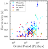 |
Fig. 7. Eccentricity-period diagram for our combined sample of stars. Cyan data points are weak Ba stars, blue data points are strong Ba stars, orange data points are CH stars, and crimson data points are the CEMP-s stars. Centroids of the populations are marked with X’s of corresponding colors. |
When applying the accretion mass as a dimension to the e − P plane, we find no significant trends with orbital period or eccentricity. We identify stars with robust abundance patterns in the large RV sample from Dimoff et al. (2024) with long orbital periods (P ≥ 1000 days) to model in deeper complexity using the STARS code in a follow-up paper; this list includes HD 201657, HD 211954, HD 224959, and HD 88562.
6. Conclusions
In this study, we have presented a grid of binary accretion models for low-mass binaries. We find that the most chosen model to explain weak Ba stars is a system that results in a 2.50 M⊙ companion, accreting a moderate amount of mass, macc ≲ 0.40 M⊙, from a 2.00 − 3.00 M⊙ AGB star. Strong Ba stars tend have lower initial masses of ∼0.6 M⊙ and accrete more material, macc ≥ 0.50 M⊙, from 2.50 M⊙ AGB stars, resulting in higher accretion efficiencies at lower initial mass ratios. Both classes of Ba stars accrete moderate to high amounts of AGB material to explain the observed surface abundance patterns. This could be due to the higher metallicities, or higher final masses where in a more massive star the convective envelope mixes more strongly than in low-mass stars. In both cases, wind mass-transfer models cannot explain the high accretion masses and efficiencies. Further modeling considering higher accretion masses may reveal a scenario that better describes the final mass distribution of the strong Ba stars.
The CH and CEMP stars are similar in many ways. They share a preference for a 2.00 − 3.00 M⊙ AGB stars and both populations show bimodal behavior with peaks at lower (∼0.80/∼1.00 M⊙) and higher masses (∼2–3 M⊙) in initial and final mass, respectively. The initial mass ratios for these metal-poor and carbon-rich systems are also somewhat bimodally split between q ≈ 0.2 and q = 1, and they tend to accrete less material (∼0.1 M⊙) from their former AGB companion compared to the metal-rich systems. These stars display lower accretion efficiencies in better agreement with the wind regime at higher mass ratios, supported by their long orbital periods and lower eccentricities. Evolution modeling including rotation is planned to track the angular momentum through the accretion process.
Acknowledgments
This project has received funding from the European Union’s Horizon 2020 research and innovation programme under grant agreement No 101008324 (ChETEC-INFRA). We graciously thank ChETEC-INFRA TNA program for providing the framework and infrastructure. Further support in funding comes from the State of Hesse within the Research Cluster ELEMENTS (Project ID 541 500/10.006) and HFHF, the Helmholz Research Academy Hessen for FAIR. We acknowledge the support of the Data Science group at the Max Planck Institute for Astronomy (MPIA) and especially Dr. Raphael Hviding and Dr. Iva Momcheva for their invaluable assistance in developing the software for this research paper. We thank our colleague Dr. Sophie van Eck for their assistance in focusing the scope of this investigation and providing feedback on this manuscript.
References
- Abate, C., Pols, O. R., Izzard, R. G., Mohamed, S. S., & de Mink, S. E. 2013, A&A, 552, A26 [NASA ADS] [CrossRef] [EDP Sciences] [Google Scholar]
- Abate, C., Pols, O. R., & Stancliffe, R. J. 2018, A&A, 620, A63 [NASA ADS] [CrossRef] [EDP Sciences] [Google Scholar]
- Allen, D. M., & Barbuy, B. 2006, A&A, 454, 895 [NASA ADS] [CrossRef] [EDP Sciences] [Google Scholar]
- Asplund, M., Grevesse, N., Sauval, A. J., & Scott, P. 2009, ARA&A, 47, 481 [NASA ADS] [CrossRef] [Google Scholar]
- Bartkevicius, A. 1996, Balt. Astron., 5, 217 [Google Scholar]
- Beers, T. C., & Christlieb, N. 2005, ARA&A, 43, 531 [NASA ADS] [CrossRef] [Google Scholar]
- Bidelman, W. P., & Keenan, P. C. 1951, ApJ, 114, 473 [Google Scholar]
- Bisterzo, S., Travaglio, C., Gallino, R., Wiescher, M., & Käppeler, F. 2014, ApJ, 787, 10 [NASA ADS] [CrossRef] [Google Scholar]
- Boffin, H. M. J., & Jorissen, A. 1988, A&A, 205, 155 [NASA ADS] [Google Scholar]
- Bond, H. E. 1974, ApJ, 194, 95 [Google Scholar]
- Bondi, H., & Hoyle, F. 1944, MNRAS, 104, 273 [Google Scholar]
- Burbidge, E. M., Burbidge, G. R., Fowler, W. A., & Hoyle, F. 1957, Rev. Mod. Phys., 29, 547 [NASA ADS] [CrossRef] [Google Scholar]
- Busso, M., Gallino, R., & Wasserburg, G. J. 1999, ARA&A, 37, 239 [Google Scholar]
- Cristallo, S., Piersanti, L., Straniero, O., et al. 2011, ApJS, 197, 17 [NASA ADS] [CrossRef] [Google Scholar]
- Cristallo, S., Straniero, O., Piersanti, L., & Gobrecht, D. 2015, ApJS, 219, 40 [Google Scholar]
- Cristallo, S., Karinkuzhi, D., Goswami, A., Piersanti, L., & Gobrecht, D. 2016, ApJ, 833, 181 [Google Scholar]
- Cseh, B., Lugaro, M., D’Orazi, V., et al. 2018, A&A, 620, A146 [NASA ADS] [CrossRef] [EDP Sciences] [Google Scholar]
- Cseh, B., Világos, B., Roriz, M. P., et al. 2022, A&A, 660, A128 [NASA ADS] [CrossRef] [EDP Sciences] [Google Scholar]
- de Castro, D. B., Pereira, C. B., Roig, F., et al. 2016, MNRAS, 459, 4299 [NASA ADS] [CrossRef] [Google Scholar]
- den Hartogh, J. W., Yagüe López, A., Cseh, B., et al. 2023, A&A, 672, A143 [NASA ADS] [CrossRef] [EDP Sciences] [Google Scholar]
- Dimoff, A. J., Hansen, C. J., Stancliffe, R., et al. 2024, A&A, 691, A128 [NASA ADS] [CrossRef] [EDP Sciences] [Google Scholar]
- Domínguez, I., Cristallo, S., Straniero, O., et al. 2011, in Why Galaxies Care about AGB Stars II: Shining Examples and Common Inhabitants, eds. F. Kerschbaum, T. Lebzelter, & R. F. Wing, ASP Conf. Ser., 445, 57 [Google Scholar]
- Edgar, R. 2004, New Astron. Rev., 48, 843 [CrossRef] [Google Scholar]
- Edvardsson, B., Andersen, J., Gustafsson, B., et al. 1993, A&A, 275, 101 [NASA ADS] [Google Scholar]
- Eggleton, P. P. 1971, MNRAS, 151, 351 [CrossRef] [Google Scholar]
- Eggleton, P. P. 1972, MNRAS, 156, 361 [NASA ADS] [Google Scholar]
- Escorza, A., Boffin, H. M. J., Jorissen, A., et al. 2017, A&A, 608, A100 [NASA ADS] [CrossRef] [EDP Sciences] [Google Scholar]
- Escorza, A., Karinkuzhi, D., Jorissen, A., et al. 2019, A&A, 626, A128 [NASA ADS] [CrossRef] [EDP Sciences] [Google Scholar]
- Gallino, R., Arlandini, C., Busso, M., et al. 1998, ApJ, 497, 388 [Google Scholar]
- Goswami, A., Aoki, W., Beers, T. C., et al. 2006, MNRAS, 372, 343 [Google Scholar]
- Goswami, A., Aoki, W., & Karinkuzhi, D. 2016, MNRAS, 455, 402 [NASA ADS] [CrossRef] [Google Scholar]
- Goswami, P. P., Rathour, R. S., & Goswami, A. 2021, A&A, 649, A49 [NASA ADS] [CrossRef] [EDP Sciences] [Google Scholar]
- Han, Z., Eggleton, P. P., Podsiadlowski, P., & Tout, C. A. 1995, MNRAS, 277, 1443 [NASA ADS] [CrossRef] [Google Scholar]
- Hansen, C. J., Andersen, A. C., & Christlieb, N. 2014, A&A, 568, A47 [NASA ADS] [CrossRef] [EDP Sciences] [Google Scholar]
- Hansen, T. T., Andersen, J., Nordström, B., et al. 2016a, A&A, 588, A3 [NASA ADS] [CrossRef] [EDP Sciences] [Google Scholar]
- Hansen, C. J., Nordström, B., Hansen, T. T., et al. 2016b, A&A, 588, A37 [NASA ADS] [CrossRef] [EDP Sciences] [Google Scholar]
- Hansen, C. J., Hansen, T. T., Koch, A., et al. 2019, A&A, 623, A128 [NASA ADS] [CrossRef] [EDP Sciences] [Google Scholar]
- Hurley, J. R., Tout, C. A., & Pols, O. R. 2002, MNRAS, 329, 897 [Google Scholar]
- Izzard, R. G., Dermine, T., & Church, R. P. 2010, A&A, 523, A10 [NASA ADS] [CrossRef] [EDP Sciences] [Google Scholar]
- Jorissen, A., Van Eck, S., Mayor, M., & Udry, S. 1998, A&A, 332, 877 [NASA ADS] [Google Scholar]
- Jorissen, A., Van Eck, S., Van Winckel, H., et al. 2016, A&A, 586, A158 [NASA ADS] [CrossRef] [EDP Sciences] [Google Scholar]
- Jorissen, A., Boffin, H. M. J., Karinkuzhi, D., et al. 2019, A&A, 626, A127 [NASA ADS] [CrossRef] [EDP Sciences] [Google Scholar]
- Jost, F. P., Molero, M., Navó, G., et al. 2025, MNRAS, 536, 2135 [Google Scholar]
- Käppeler, F., Gallino, R., Bisterzo, S., & Aoki, W. 2011, Rev. Mod. Phys., 83, 157 [Google Scholar]
- Karakas, A. I., & Lattanzio, J. C. 2014, PASA, 31, e030 [NASA ADS] [CrossRef] [Google Scholar]
- Karakas, A. I., Tout, C. A., & Lattanzio, J. C. 2000, MNRAS, 316, 689 [NASA ADS] [CrossRef] [Google Scholar]
- Karinkuzhi, D., & Goswami, A. 2014, MNRAS, 440, 1095 [Google Scholar]
- Karinkuzhi, D., & Goswami, A. 2015, MNRAS, 446, 2348 [NASA ADS] [CrossRef] [Google Scholar]
- Karinkuzhi, D., Van Eck, S., Jorissen, A., et al. 2018, A&A, 618, A32 [NASA ADS] [CrossRef] [EDP Sciences] [Google Scholar]
- Karinkuzhi, D., Van Eck, S., Jorissen, A., et al. 2021, A&A, 654, A140 [NASA ADS] [CrossRef] [EDP Sciences] [Google Scholar]
- Keenan, P. C. 1942, ApJ, 96, 101 [NASA ADS] [CrossRef] [Google Scholar]
- Krynski, P., Siess, L., Jorissen, A., & Davis, P. J. 2025, A&A, 697, A179 [NASA ADS] [CrossRef] [EDP Sciences] [Google Scholar]
- Liu, Z.-W., Stancliffe, R. J., Abate, C., & Matrozis, E. 2017, ApJ, 846, 117 [Google Scholar]
- Lombardo, L., Hansen, C. J., Rizzuti, F., et al. 2025, A&A, 693, A293 [NASA ADS] [CrossRef] [EDP Sciences] [Google Scholar]
- Lu, P. K. 1991, AJ, 101, 2229 [CrossRef] [Google Scholar]
- Lu, P. K., Dawson, D. W., Upgren, A. R., & Weis, E. W. 1983, ApJS, 52, 169 [CrossRef] [Google Scholar]
- Lucatello, S., Tsangarides, S., Beers, T. C., et al. 2005, ApJ, 625, 825 [NASA ADS] [CrossRef] [Google Scholar]
- Lugaro, M., Pignatari, M., Reifarth, R., & Wiescher, M. 2023, Annu. Rev. Nucl. Part. Sci., 73, 315 [NASA ADS] [CrossRef] [Google Scholar]
- Masseron, T., Johnson, J. A., Plez, B., et al. 2010, A&A, 509, A93 [NASA ADS] [CrossRef] [EDP Sciences] [Google Scholar]
- Matrozis, E., & Stancliffe, R. J. 2016, A&A, 592, A29 [NASA ADS] [CrossRef] [EDP Sciences] [Google Scholar]
- Matrozis, E., Abate, C., & Stancliffe, R. J. 2017, A&A, 606, A137 [NASA ADS] [CrossRef] [EDP Sciences] [Google Scholar]
- McClure, R. D. 1984, ApJ, 280, L31 [Google Scholar]
- McClure, R. D., & Woodsworth, A. W. 1990, ApJ, 352, 709 [Google Scholar]
- McClure, R. D., Fletcher, J. M., & Nemec, J. M. 1980, ApJ, 238, L35 [Google Scholar]
- Mohamed, S., & Podsiadlowski, P. 2007, in 15th European Workshop on White Dwarfs, eds. R. Napiwotzki, & M. R. Burleigh, ASP Conf. Ser., 372, 397 [Google Scholar]
- Mohamed, S., & Podsiadlowski, P. 2012, Balt. Astron., 21, 88 [Google Scholar]
- Norris, J. E., Ryan, S. G., & Beers, T. C. 1997, ApJ, 488, 350 [CrossRef] [Google Scholar]
- Pereira, C. B., Sales Silva, J. V., Chavero, C., Roig, F., & Jilinski, E. 2011, A&A, 533, A51 [NASA ADS] [CrossRef] [EDP Sciences] [Google Scholar]
- Pols, O. R., Tout, C. A., Eggleton, P. P., & Han, Z. 1995, MNRAS, 274, 964 [Google Scholar]
- Prantzos, N., Abia, C., Limongi, M., Chieffi, A., & Cristallo, S. 2018, MNRAS, 476, 3432 [Google Scholar]
- Purandardas, M., Goswami, A., Goswami, P. P., Shejeelammal, J., & Masseron, T. 2019, MNRAS, 486, 3266 [Google Scholar]
- Romano, D., Karakas, A. I., Tosi, M., & Matteucci, F. 2010, A&A, 522, A32 [NASA ADS] [CrossRef] [EDP Sciences] [Google Scholar]
- Roriz, M. P., Lugaro, M., Pereira, C. B., et al. 2021a, MNRAS, 507, 1956 [NASA ADS] [CrossRef] [Google Scholar]
- Roriz, M. P., Lugaro, M., Pereira, C. B., et al. 2021b, MNRAS, 501, 5834 [NASA ADS] [CrossRef] [Google Scholar]
- Roriz, M. P., Holanda, N., da Conceição, L. V., et al. 2024, AJ, 167, 184 [Google Scholar]
- Ryan, S. G., Norris, J. E., & Beers, T. C. 1996, ApJ, 471, 254 [Google Scholar]
- Schroder, K.-P., Pols, O. R., & Eggleton, P. P. 1997, MNRAS, 285, 696 [NASA ADS] [CrossRef] [Google Scholar]
- Stancliffe, R. J. 2005, Ph.D. Thesis, University of Cambridge, UK [Google Scholar]
- Stancliffe, R. J. 2015, in Why Galaxies Care about AGB Stars III: A Closer Look in Space and Time, eds. F. Kerschbaum, R. F. Wing, & J. Hron, ASP Conf. Ser., 497, 253 [Google Scholar]
- Stancliffe, R. J. 2021, MNRAS, 505, 5554 [NASA ADS] [CrossRef] [Google Scholar]
- Stancliffe, R. J., & Eldridge, J. J. 2009, MNRAS, 396, 1699 [NASA ADS] [CrossRef] [Google Scholar]
- Stancliffe, R. J., & Glebbeek, E. 2008, MNRAS, 389, 1828 [Google Scholar]
- Stancliffe, R. J., Glebbeek, E., Izzard, R. G., & Pols, O. R. 2007, A&A, 464, L57 [NASA ADS] [CrossRef] [EDP Sciences] [Google Scholar]
- Stancliffe, R. J., Fossati, L., Passy, J. C., & Schneider, F. R. N. 2015, A&A, 575, A117 [NASA ADS] [CrossRef] [EDP Sciences] [Google Scholar]
- Starkenburg, E., Shetrone, M. D., McConnachie, A. W., & Venn, K. A. 2014, MNRAS, 441, 1217 [Google Scholar]
- Straniero, O., Gallino, R., & Cristallo, S. 2006, Nucl. Phys. A, 777, 311 [NASA ADS] [CrossRef] [Google Scholar]
- Udry, S., Jorissen, A., Mayor, M., & Van Eck, S. 1998, A&AS, 131, 25 [NASA ADS] [CrossRef] [EDP Sciences] [Google Scholar]
- Warner, B. 1965, MNRAS, 129, 263 [Google Scholar]
Appendix A: The Model Grid
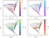 |
Fig. A.1. Our computed grid of evolutionary models in the HR diagram, displaying every 5th model in gray. Selected models are highlighted to show the range of parameters across the grid. Panel (a) shows the varying metallicities of our models, with purple models at lower metallicity and orange models at higher metallicities. These are spread across the Kiel diagram. On the giant branch, metal-rich evolutionary tracks fall to the right side of the giant branch toward cooler temperatures, where metal-poor giants are on the left side at higher temperatures. Panel (b) shows the range of initial masses, with lower initial masses in blue and higher initial masses in pink. Lower initial-mass models appear toward the bottom and right of the panel, and higher initial-mass models to top and the left. Panel (c) shows the range of final masses. The highlighted evolutionary tracks are for a fixed metallicity of -0.15, with green and yellow models showing higher mass and blue models showing lower mass. This parameter follows the same general trend as the initial masses. Panel (d) displays an example of the varying accretion mass in our models. The highlighted tracks begin at different initial masses all resulting in mfinal = 2.50 M⊙, at a metallicity of [Fe/H] = -0.15. Black tracks show higher accretion masses, and yellow tracks show lower amounts of accretion. |
All Tables
All Figures
|
Fig. 1. Kiel diagram showing surface gravities and effective temperatures for the collected observational sample. Blue data points are strong Ba stars, cyan data points are weak Ba stars, orange data points are CH stars, and red data points are CEMP-s stars. Surface parameters and abundances are collected from Dimoff et al. (2024), de Castro et al. (2016), Roriz et al. (2021a), Goswami et al. (2006, 2016, 2021), Karinkuzhi & Goswami (2014, 2015). |
| In the text | |
|
Fig. 2. Left: Evolutionary tracks for a sample of stars with mfinal = 2.50 M⊙ at [Fe/H] = −0.15 with varying initial masses and accretion masses, with accretion phases for each model highlighted in blue. Right: Relative surface abundance of the s-process element Ba with log10(Age/yr). The abundance is elevated after the accretion phase, and after the onset of first dredge-up the surface abundance is diluted. |
| In the text | |
|
Fig. 3. Example Kippenhahn diagram for a 2.00 M⊙ star accreting 0.50 M⊙ of material from a 2.50 M⊙ AGB star at a metallicity of [Fe/H] = − 0.15. Green colors denote convective regions, and purple colors denote radiative regions, determined by the computed difference in the radiative and adiabatic transfer gradients. In the total mass on the y axis, the accretion phase can be identified by the increase in mass. The upper x axis shows log10(Age/yr), and the lower x axis shows the model number, which is highly nonlinear with respect to time. |
| In the text | |
|
Fig. 4. Kiel diagrams and abundance fits for the weak Ba star PV UMa, the strong Ba star HD 123949, and the CEMP-s star CS 29512-073, each showing the three best-fitting models and their associated χ2 values. |
| In the text | |
|
Fig. 5. Histograms of model parameters for the different classes of stars in our investigation. Dark blue regions are strong Ba stars, cyan regions are weak Ba stars, red regions are CEMP-s stars, and orange regions are CH stars. |
| In the text | |
|
Fig. 6. Computed accretion efficiencies for our sample populations. Purple-blue contours are the strong Ba stars, and the green contours are the weak Ba stars. Red-yellow contours are our carbon-enhanced sample, including both CH and CEMP-s stars. |
| In the text | |
|
Fig. 7. Eccentricity-period diagram for our combined sample of stars. Cyan data points are weak Ba stars, blue data points are strong Ba stars, orange data points are CH stars, and crimson data points are the CEMP-s stars. Centroids of the populations are marked with X’s of corresponding colors. |
| In the text | |
|
Fig. A.1. Our computed grid of evolutionary models in the HR diagram, displaying every 5th model in gray. Selected models are highlighted to show the range of parameters across the grid. Panel (a) shows the varying metallicities of our models, with purple models at lower metallicity and orange models at higher metallicities. These are spread across the Kiel diagram. On the giant branch, metal-rich evolutionary tracks fall to the right side of the giant branch toward cooler temperatures, where metal-poor giants are on the left side at higher temperatures. Panel (b) shows the range of initial masses, with lower initial masses in blue and higher initial masses in pink. Lower initial-mass models appear toward the bottom and right of the panel, and higher initial-mass models to top and the left. Panel (c) shows the range of final masses. The highlighted evolutionary tracks are for a fixed metallicity of -0.15, with green and yellow models showing higher mass and blue models showing lower mass. This parameter follows the same general trend as the initial masses. Panel (d) displays an example of the varying accretion mass in our models. The highlighted tracks begin at different initial masses all resulting in mfinal = 2.50 M⊙, at a metallicity of [Fe/H] = -0.15. Black tracks show higher accretion masses, and yellow tracks show lower amounts of accretion. |
| In the text | |
Current usage metrics show cumulative count of Article Views (full-text article views including HTML views, PDF and ePub downloads, according to the available data) and Abstracts Views on Vision4Press platform.
Data correspond to usage on the plateform after 2015. The current usage metrics is available 48-96 hours after online publication and is updated daily on week days.
Initial download of the metrics may take a while.