| Issue |
A&A
Volume 701, September 2025
|
|
|---|---|---|
| Article Number | A24 | |
| Number of page(s) | 13 | |
| Section | Cosmology (including clusters of galaxies) | |
| DOI | https://doi.org/10.1051/0004-6361/202555778 | |
| Published online | 28 August 2025 | |
Signatures of fuzzy dark matter inside radial critical curves
1
Instituto de Física de Cantabria (CSIC-UC), Avda. Los Castros s/n, 39005, Santander, Spain
2
Department of Physics, University of the Basque Country (UPV/EHU), 48080, Bilbao, Spain
3
Donostia International Physics Center, DIPC, Basque Country, San Sebastián, 20018, Spain
4
Department of Physics, The University of Hong Kong, Pokfulam Road, Hong Kong
5
Ikerbasque, Basque Foundation for Science, Bilbao, Spain
⋆ Corresponding author: This email address is being protected from spambots. You need JavaScript enabled to view it.
Received:
2
June
2025
Accepted:
16
July
2025
Abstract
We investigated the strong gravitational lensing properties of fuzzy dark matter (FDM) haloes, focussing on the magnification properties near radial critical curves (CCs). Using simulated lenses, we computed magnification maps for a range of axion masses and halo configurations. We show that FDM produces enhanced central magnification and secondary CCs that are not easily reproduced by standard cold dark matter (CDM), even when subhaloes are included. The strength and scale of these effects depend primarily on the de Broglie wavelength, which is governed by the axion and halo masses. We find that axion masses in the range mψ ∼ 10−22–10−21 eV in galaxy-mass haloes lead to distinctive magnification distributions. Our results suggest that observations of highly magnified, compact sources near radial arcs, such as quasars or supernovae, could serve as a powerful test for the presence of FDM.
Key words: galaxies: halos / dark matter
© The Authors 2025
 Open Access article, published by EDP Sciences, under the terms of the Creative Commons Attribution License (https://creativecommons.org/licenses/by/4.0), which permits unrestricted use, distribution, and reproduction in any medium, provided the original work is properly cited.
This article is published in open access under the Subscribe to Open model. This email address is being protected from spambots. You need JavaScript enabled to view it. to support open access publication.
1. Introduction
The lambda-cold dark matter cosmological model (ΛCDM) provides the most successful description of our Universe to date (Planck Collaboration VI 2020). In this framework, the energy density of the Universe consists predominantly of mysterious dark energy (∼70%), which drives the accelerated expansion (observed primarily at z < 1). The remaining ∼30% corresponds to matter, of which only about 5% is the familiar baryonic matter, while the remaining ∼25% is attributed to the elusive cold dark matter (CDM). Although the gravitational effects of CDM have been evident for decades, its true nature remains a mystery in modern cosmology. Although the ΛCDM model accurately reproduces the large-scale structure of the universe, it still faces significant challenges on small scales (Del Popolo & Le Delliou 2017), particularly at scales ≲1 Mpc. These small-scale problems include, among others, the core–cusp problem (Moore 1994; Moore et al. 1999; Flores & Primack 1994; Oh et al. 2011; Gentile et al. 2004), the missing satellites problem (Moore et al. 1999; Klypin et al. 1999), and the too-big-to-fail problem (Boylan-Kolchin et al. 2011, 2012).
Some progress has been made in addressing the core–cusp tension through high-resolution cosmological simulations of disc galaxies that incorporate strong baryonic feedback, particularly supernova-driven outflows, and high star formation thresholds (Guedes et al. 2011; McCarthy et al. 2012; Brook et al. 2012). However, the extent to which these mechanisms can alleviate other small-scale issues, such as core formation or satellite abundances, remains debated (Schaller et al. 2015).
The fundamental nature of dark matter remains unknown. Alternative scenarios to CDM, such as self-interacting dark matter (Tulin & Yu 2018) or warm dark matter (Viel et al. 2013), have been proposed to account for persistent discrepancies between the predictions of standard CDM and observations on small scales. Modifications to the ΛCDM paradigm have also been proposed to address these small-scale issues. Among the leading CDM candidates are weakly interacting massive particles (WIMPs) (Arcadi et al. 2018), which are fermionic and behave as discrete particles, and wave dark matter (ψDM), a bosonic alternative composed of ultralight particles with masses below 10 eV (Hui 2021; Ferreira 2021). This latter model reflects the particle–wave duality of quantum mechanics, as the de Broglie wavelength of the particles exceeds their average separation in galaxies, allowing dark matter to be treated effectively as a classical wave.
In particular, fuzzy dark matter (FDM) is a kind of ψDM model that is non-self-interacting, non-relativistic, and extremely light, with a mass in the range 10−23–10−20 eV (Hu et al. 2000; Hui et al. 2017). One of the key advantages of FDM is its ability to address two of the aforementioned problems: the core–cusp problem, through the formation of a solitonic core in galaxies (Schive et al. 2014; Mocz et al. 2017), and the missing satellite problem, via the suppression of structure formation below the de Broglie scale (Robles et al. 2015); Schive:2015kza; Kulkarni:2020pnb. This suppression is reminiscent of warm dark-matter models. However, FDM is still CDM and is indistinguishable from standard CDM predictions on large scales (Schive et al. 2014); Hui:2021tkt.
The FDM prediction of solitonic cores and the suppression of small-scale structure in the linear regime (Hui 2021) make this model highly testable and subject to numerous current constraints. Observations of the early Universe (Zhang et al. 2024), axion detection experiments (Aja et al. 2022; Leung et al. 2019), and searches for astrophysical-related phenomena (Eberhardt et al. 2024; Pinetti 2025) have been used to place general limits on the existence of ψDM. In the case of FDM, the usual mass range, around 10−22 eV, has been constrained by the small-scale spatial fluctuations measured via the Lyman-α forest (Iršič et al. 2017; Kobayashi et al. 2017; Armengaud et al. 2017), by galaxy dynamics and internal structure (Nadler et al. 2021) and by the sizes and stellar radial velocities of some ultra-faint dwarf galaxies (Dalal & Kravtsov 2022). These constraints disfavour an axion mass near the commonly adopted value of 10−22 eV, yet they are subject to systematic uncertainties. These arise from limited data and poorly understood baryonic physics (Hui 2021) or from the lack of full-wave simulations that could capture higher-order effects (Dalal & Kravtsov 2022). Properly accounting for these factors could potentially relax the current bounds. Regardless of the strength of these constraints, it is crucial to develop complementary approaches based on independent methods to better assess and mitigate systematic uncertainties.
Gravitational lensing presents itself as an excellent tool to probe axion masses and test the viability of FDM as a dark matter candidate (Laroche et al. 2022; Amruth et al. 2023; Powell et al. 2023; Broadhurst et al. 2025). Since lensing traces the underlying projected mass distribution, it is sensitive to substructure on different scales, as predicted by various dark-matter models. Axion masses of around 10−22 eV in FDM are particularly notable for producing de Broglie wavelengths that give rise to mass density fluctuations on parsec to kiloparsec scales in galaxy clusters and galaxy-scale lens systems, respectively. These fluctuations lead to distinctive patterns in the mass distribution compared with the conventional smooth global profiles expected from standard CDM. Such differences have already been proposed as solutions for discrepancies between observational data and the best-fitting canonical CDM-based lensing models (Amruth et al. 2023), such as the long-standing flux-ratio anomalies (Keeton et al. 2003; Goldberg et al. 2010; Xu et al. 2015; Shajib et al. 2019), the position anomalies in radio observations (Spingola et al. 2018; Hartley et al. 2019), or the asymmetry in microlensed stars in galaxy clusters (Broadhurst et al. 2025).
In this paper, we develop a lensing framework tailored to FDM distributions in galaxy-scale systems, with a particular focus on deviations in their magnification patterns compared with the case of standard CDM haloes. We focus on radial critical curves (CCs), which are often neglected in the literature, as smooth models predict demagnified central images, and radial images are also less common than their tangential counterparts. However, certain small-scale objects (smaller than the de Broglie wavelength), such as active galactic nuclei, quasi-stellar objects (QSOs), or supernovae, can be bright enough to be observed even at modest magnification factors and be sensitive to magnification changes due to FDM fluctuations. However, perhaps the most important fact is that near the CCs, the differences between standard CDM and FDM can be accentuated. The radial critical region corresponds to the portion of the lens where (1 − κ)+γ = ε ≈ 0, where κ is the convergence, γ is the shear, and ε is an arbitrarily small number. In this region, since γ > 0 always, it must follow that κ > 1. In the classical CDM scenario, adding a substructure increases the value of κ, thereby making the term (1 − κ) more negative and, in most cases, leading to a reduction in magnification (μ ∝ ε−1). In contrast, in FDM, negative mass fluctuations (with respect to the mean) relax the condition for criticality and increase the probability of larger magnification (smaller |ε|). In other words, this simple reasoning leads to the expectation of a higher number of highly magnified objects in the vicinity of the radial CC region in FDM models compared to standard CDM. In this work, we provide a quantitative assessment of the differences between canonical CDM and FDM near radial CCs in terms of their magnification statistics. Here, we demonstrate that FDM predicts a magnification distribution near the centre of haloes, specifically around radial CCs, that differs significantly from that predicted by standard CDM, even when including subhaloes as small-scale perturbers. This behaviour represents an effect unique to FDM, providing a promising avenue to test FDM models as an alternative to canonical CDM.
This paper is structured as follows. Section 2 introduces the basics of gravitational lensing, with a particular emphasis on magnification, the observable we propose to use for distinguishing an FDM universe from one governed by the classical representation of CDM. In Section 3, we describe the various mass profiles implemented in our simulations, which are later compared in terms of their magnification properties. In Section 4, we present the methodology followed in this work. The results of our analysis, highlighting the differences among the models and the tests employed, are presented in Section 5. In Section 6, we discuss the implications of our findings and the potential of magnification as a tool for discriminating between dark matter models. Finally, our main conclusions are summarised in Section 7. We assume the Planck 18 cosmological model (Planck Collaboration VI 2020) with Ωm = 0.31, Λ = 0.69, and h = 0.676 (100 km s−1 Mpc−1). In this work, we study the differences between FDM and the standard CDM description within the ΛCDM framework. Without loss of generality, we refer to the latter simply as CDM throughout the paper, even though FDM is itself a form of CDM.
2. Lensing formalism
In this section, we briefly introduce the gravitational lensing formalism (Schneider et al. 1992), focussing on the gravitational lensing effect caused by galaxy lenses. These lenses are typically described by a Navarro–Frenk–White (NFW) dark matter halo (Navarro et al. 1996, 1997), consistent with both observations and hydrodynamic simulations (in CDM). A Sérsic profile was adopted for the contribution from baryons. Finally, for the FDM mass profiles, we included the soliton structure and density fluctuations on top of an NFW profile.
The formalism presented here is, nonetheless, mass-model independent and can be readily applied to any deflecting structure, including, but not limited to, NFW or Sérsic profiles. In addition, when working with complex mass models, we can take advantage of the deflection angle linearity, i.e. the total deflection angle can be expressed as the sum of the deflection angle of each component. Specifically, if the total mass distribution can be expressed as
 (1)
(1)
then the total deflection angle is
 (2)
(2)
where αi(θ) is the deflection angle at the position θ generated by the mass distribution Σi.
The position of a lensed image β and the corresponding source position θ are connected through the lens equation
 (3)
(3)
where α is the deflection angle induced at θ by a lens with a surface mass density Σ(θ). Since α depends on θ, the equation is generally non-linear, often admitting multiple image positions for a given source location and lacking an analytical solution in most cases.
The deflection angle is derived from the effective lensing potential:
 (4)
(4)
where Dd, Ds, and Dds represent the angular diameter distances to the lens, to the source, and between the lens and the source, respectively. The function ϕ denotes the Newtonian potential of the lens. The deflection is then given by
 (5)
(5)
and the Laplacian of ψ is related to the surface mass density through
 (6)
(6)
where G is the gravitational constant, and κ is the convergence, defined as the dimensionless surface mass density relative to the critical value Σcrit.
Gravitational lensing also modifies the shape and size of background sources. These distortions are encoded in the Jacobian matrix
 (7)
(7)
which is the inverse of the magnification tensor M.
3. Mass profiles
In the previous section, we introduced the lensing formalism for a generic mass distribution Σ(θ), which is the 2D projection of a generic ρ(θ, z) 3D profile, obtained by integrating the density along the line of sight z. In this section, we summarise the mass distributions used in this work for both the particle description of CDM and the wave-like FDM models.
3.1. Navarro-Frenk-White profile
Simulations have shown that, under the ΛCDM paradigm, the power spectrum of the density perturbations, combined with the collisionless nature of CDM, point to cuspy dark haloes with density profiles scaling as ρDM(r)∝r−1. These profiles are well described by the NFW parameterisation (Navarro et al. 1996, 1997), from very massive galaxy clusters (M ∼ 1015 M⊙) to galaxies with masses around M ∼ 1011–1012 M⊙. Simulations of FDM haloes also show an NFW profile modulated by a central solitonic core and density fluctuations characteristic of its wave nature (Schive et al. 2014).
The NFW profile is a radial function given by
 (8)
(8)
where the two parameters, ρs and rs, are the characteristic density and the scale radius of the halo. Lower-mass haloes are usually well described by NFW profiles as well, but the core–cusp problem arises: the central density tends to an almost constant value rather than rising steeply at the innermost radii. Fuzzy dark matter (FDM) offers a natural solution to this discrepancy through solitonic structures, as seen in numerical simulations (Schive et al. 2014; Liao et al. 2024). The characteristic density, ρs, can also be expressed as a function of the concentration parameter
![Mathematical equation: $$ \begin{aligned} \rho _s=\frac{200}{3}\rho _{\rm crit}\frac{c^3}{\left[\ln {(1+c)} - \frac{c}{1+c} \right]}\cdot \end{aligned} $$](/articles/aa/full_html/2025/09/aa55778-25/aa55778-25-eq9.gif) (9)
(9)
The concentration parameter, c, is simply the ratio between the radius, r200, and the scale radius of the halo (c = r200/rs), and scales with the mass of the halo roughly as M−0.1 (Dutton & Macciò 2014). The radius r200 encloses an average density 200 times that of the critical density:
![Mathematical equation: $$ \begin{aligned} r_{200} = \frac{1.63\times 10^{-2}}{(1+ z)h}\left(\frac{M_{200}}{h^{-1}\,M_\odot }\right)^{1/3} \left[\frac{\Omega _0}{\Omega (z)}\right]^{-1/3}\,\mathrm{kpc}. \end{aligned} $$](/articles/aa/full_html/2025/09/aa55778-25/aa55778-25-eq10.gif) (10)
(10)
Here, h is the dimensionless Hubble parameter, and M200 is the mass enclosed within the sphere of radius r200, also commonly used to parametrise the halo, analogously to ρs and rs. Defining x ≡ r/rs, the simplicity of the NFW profile, specifically its radial symmetry, allows an analytical derivation of its surface mass density:
 (11)
(11)
The limit at x = 1 is finite:  . The deflection angle is then given by
 (12)
(12)
with the auxiliary function h(x) defined as
![Mathematical equation: $$ \begin{aligned} h(x) = \ln \left(\frac{x}{2}\right) + {\left\{ \begin{array}{ll} \frac{2}{\sqrt{x^2 - 1}} \arctan \sqrt{\frac{x - 1}{x + 1}},&x > 1 \\ [3pt] \frac{2}{\sqrt{1 - x^2}} {\text{ arctanh}}\sqrt{\frac{1 - x}{1 + x}},&x < 1 \\ [3pt] 1,&x = 1. \end{array}\right.} \end{aligned} $$](/articles/aa/full_html/2025/09/aa55778-25/aa55778-25-eq14.gif) (13)
(13)
The mass profile presented here is valid for CDM haloes and subhaloes according to CDM predictions. This profile serves as the central baseline model for FDM; further distinctions are outlined in the following subsection.
3.2. FDM profile
Simulations show that FDM halo profiles are composed of three distinct components. First, a baseline NFW-like profile, as described in the previous subsection. Second, a central solitonic core that produces a flat inner density profile and naturally addresses the core–cusp problem. Together, these two components constitute the smooth mass distribution of the halo. Third, small-scale wavelike density fluctuations, arising from the quantum nature of the field, introduce granularity beyond the smooth profile. The first component was discussed previously; here, we focus on the solitonic core and small-scale wave-like density fluctuation, which are unique features of FDM.
3.2.1. Soliton
Solitons are stationary, spherically symmetric ground-state solutions of the Schrödinger–Poisson equation. They appear as a central flat density, as opposed to the cuspy inner density of NFW haloes. Solitons exhibit a time-variable centre offset (1 kpc) referred to as the soliton random walk, which arises from wave interference (Schive et al. 2020). This random walk has a timescale of approximately 100 Myr (Schive et al. 2020), which is too large to affect the lensing systems that we observe. Solitons are typically characterised by a single parameter, Ms, the soliton mass. The so-called soliton–halo relation expresses the soliton mass in terms of its host halo and redshift. This relation was first identified in cosmological simulations (Schive et al. 2014). More recent studies (Liao et al. 2024) confirm that it takes the form  , where mψ is the axion mass, Mh is the halo mass, and zh is its redshift. Although this relation has been confirmed by other studies, some results suggest different relations, such as Ms ∝ Mh5/9(Mocz et al. 2017). A large scatter in the soliton–halo relation has been reported, suggesting that the relation may not be universal and remains an open question. For the remainder of this work, we assume a soliton–halo relation as found by Schive et al. (2014) (Ms ∝ Mh1/3), specifically in the form reported by Liao et al. (2024), since their simulations cover higher halo masses that had not been explored in previous works.
The soliton mass density profile is given by
 (14)
(14)
where
 (15)
(15)
The radius rc is defined as the distance at which the density drops to half its central value.
The smooth component of the FDM model mass density profile, as shown in Fig. 1, is then
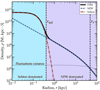 |
Fig. 1. Radial profile of an FDM halo (Mh = 7 × 10¹¹ M⊙ and mψ = 10−22 eV at z = 0.9), neglecting quantum fluctuations (solid black line). The inner profile of the halo is dominated by the soliton structure (dot-dashed red line). At r = rsol, the profile transitions to a standard NFW dark matter halo (dashed blue line). The radial variance of the fluctuations, given by Eq. (21) (dot-dashed grey line) is shown in arbitrary units. |
 (16)
(16)
where rsol is the transition radius between models, which can be found numerically from the condition ρsol(rsol)=ρNFW(rsol). It is typically a few times rc: 2.5 ≲ rsol/rc ≲ 3.5 (Mocz et al. 2017); Chiang:2021uvt; Furlanetto:2024qsb.
Finally, the 2D projection of the mass density profile (without quantum fluctuations) can be obtained by numerically integrating along the line of sight:
 (17)
(17)
Here, r is defined as the radial distance within the lens plane and z is the tangential direction to the plane.
3.2.2. FDM fluctuations
In the preceding subsections, we described the smooth component of the FDM profile, which is composed of a main NFW halo in the outskirts and a soliton profile in the central region. In addition, FDM exhibits density clumps roughly separated by half the de Broglie wavelength, which depends on the axion and halo masses:
 (18)
(18)
Following Amruth et al. (2023), Kawai et al. (2022), Dalal et al. (2021), we assumed that the integrated column density fluctuations along the line of sight can be well approximated as a Gaussian random field (GRF). This GRF can be drawn as a random realisation from the power spectrum
 (19)
(19)
where
 (20)
(20)
is the effective halo size, which contains information on the density dispersion along the line of sight, Z. Here, ρh is the average local mass density of the halo. This field is modulated by a radial variance function that depends on x:
![Mathematical equation: $$ \begin{aligned} \sigma ^2(x)\approx \left\{ \begin{array}{ll} \displaystyle \frac{\kappa _s^2}{r_s \lambda _{\mathrm{dB} }} \left[\frac{\pi }{x}- \frac{1}{(x^2 - 1)^3} \left( \frac{6x^4 - 17x^2 + 26}{3} +\right. \right. \\ [8pt] \left. \left. \qquad \quad \displaystyle \frac{2x^6 - 7x^4 + 8x^2 - 8}{\sqrt{1 - x^2}} \, \mathrm{sech} ^{-1}(x) \right) \right],&x < 1 \\ [5pt] \displaystyle \frac{\kappa _s^2}{r_s \lambda _{\mathrm{dB} }} \left[ \frac{\pi }{x}- \frac{1}{(x^2 - 1)^3} \left( \frac{6x^4 - 17x^2 + 26}{3} +\right. \right. \\ [8pt] \left. \left. \qquad \quad \displaystyle \frac{2x^6 - 7x^4 + 8x^2 - 8}{\sqrt{x^2 - 1}} \, \sec ^{-1}(x) \right) \right],&x > 1 \end{array} \right., \end{aligned} $$](/articles/aa/full_html/2025/09/aa55778-25/aa55778-25-eq23.gif) (21)
(21)
where the limit at x ≡ r/rs = 1 is  and κs ≡ ρsrs/Σcrit is the characteristic convergence.
The surface mass density of the FDM can then be drawn as a random realisation given P(k) in Eq. (19) modulated by the radial variance given by Eq. (21). Neither the soliton nor the GRF density fluctuations admit analytical expressions for their deflection angles and must therefore be computed numerically.
3.3. Sérsic profile
The profiles shown so far describe dark matter haloes that are in good agreement with the data. Such haloes account for approximately 90% of the total mass of the galaxies, while the other 10% consists of baryons, whose mass can be traced from the light distribution. The effect of the baryons is a dampening of the FDM mass surface density fluctuations, as found by Amruth et al. (2023). In the present study, we considered only a modest dampening factor of ∼20% to show the differences between CDM and FDM.
The surface brightness of elliptical galaxies, bulges, and discs of spiral galaxies is best fitted by a S’ersic profile (r1/n), where n is a free parameter known as the Sérsic index n. Although not a 3D mass profile, the S’ersic profile is a good approximation of the 2D projection of the mass distribution, assuming a homogeneous light-to-mass ratio. Specifically, this circularly symmetric mass profile is expressed as
![Mathematical equation: $$ \begin{aligned} \Sigma (r) = \Upsilon \, I_e \exp \left\{ -b(n) \left[ \left( \frac{r}{r_e} \right)^{1/n} - 1 \right] \right\} , \end{aligned} $$](/articles/aa/full_html/2025/09/aa55778-25/aa55778-25-eq25.gif) (22)
(22)
where Υ is the light-to-mass ratio of the galaxy, Ie is the luminosity density at the effective radius re, and b(n) is a constant defined so that the luminosity enclosed within re equals half of the total luminosity. The Sérsic index, n, determines the concentration of the profile, with lower values corresponding to shallower inner slopes and steeper outer fall-offs. Typical values include n ≈ 1 for exponential discs in spiral galaxies, and n ≈ 4 for bulges and elliptical galaxies, corresponding to the de Vaucouleurs profile.
As in the NFW profile, we defined a dimensionless quantity x = (r/re)1/n. As shown in Eq. (6), the convergence is half the Laplacian of the lensing potential. The lensing potential, ψ, can be obtained by solving that equation, and the deflection angle is then the gradient of the lensing potential. To derive an analytical expression for the Sérsic profile, we followed the procedure of Cardone (2004). The deflection angle takes the form
![Mathematical equation: $$ \begin{aligned} \alpha (x) = 2\alpha _e\, x^{-n} \left[1 - \frac{\Gamma (2n, bx)}{\Gamma (2n)}\right], \end{aligned} $$](/articles/aa/full_html/2025/09/aa55778-25/aa55778-25-eq26.gif) (23)
(23)
where αe is the deflection angle at r = re, whose value is given by
 (24)
(24)
in arcsec units. The quantity κe is defined as κe = Υ Ie/Σcrit, where Γ(a, z) is the incomplete gamma function and Γ(a) is the actual gamma function. The parameter b(n) can be found from the equation
 (25)
(25)
Tabulated values of b(n) for n ∈ {1, …, 15} can be found in Mazure & Capelato (2002).
4. Methodology
In this work, we assumed different mock lenses by varying their halo masses and ellipticities, and by adding various small-scale perturbers to study the differences in radial magnification arcs between CDM and FDM for different axion masses. For each case, we computed the deflection angles numerically or, when possible, analytically. We then added them linearly and computed the magnification in the lens plane following Eq. (7):
 (26)
(26)
The deflection angles for the Sérsic and NFW profiles were obtained analytically (Eqs. (12) and (23)), significantly speeding up the process. The soliton and FDM fluctuations were computed numerically, according to Eqs. (1) and (2). Each pixel was treated as a point lens, and the total deflection angle was estimated via a convolution between the mass and distance kernels using the fast Fourier transform (Cooley & Tukey 1965). For each case, we simulated a field of view (FOV) ranging from three to seven times the Einstein radius of the lens to fully cover the CCs. This variable FOV is motivated by the ellipticity of the lens, which stretches the CCs along one axis while compressing them along the other. We assumed that all lenses were circularly symmetric when computing the deflection angle and added ellipticity afterwards as
 (27)
(27)
where F is a circularly symmetric function, x and y are the Cartesian coordinates of the lens plane,  is the radial distance within the plane, and e ≡ 1 − b/a is the ellipticity, with a and b representing the major and minor semi-axes of the ellipse.
First, for a mock lens, we constructed the smooth CDM lens model by combining an NFW dark matter halo with a Sérsic profile representing the baryonic component of the galaxy. We then computed the deflection angles for each component, added them linearly, and obtained the resulting magnification map. Additionally, we assumed a fiducial axion mass. For practical reasons, we selected mψ from three values, mψ ∈ 0.4, 1, 10 × 10−22 eV: the lower limit was motivated by the conservative constraint on the axion mass from Chiang et al. (2023). The middle value was chosen for historical reasons, as it is the most commonly adopted in ultralight axion FDM studies and is found by many studies to reproduce the observed properties of multiply lensed images (Amruth et al. 2023; Laroche et al. 2022) or the innermost kinematics of dwarf galaxies (Broadhurst et al. 2020). The upper value lies in a regime in which current constraints remain weak.
We considered three different halo masses, M200: a fiducial mass of 7 × 10¹¹ M⊙ as in Amruth et al. (2023), a smaller halo of 3 × 10¹¹ M⊙, and a massive halo of 4 × 10¹² M⊙. The combination of three axion masses and three halo masses yields a total of nine models, as shown in Table 1. We also adopted the lens parameters from Amruth et al. (2023) for the HS 0810+2554 system, using zl = 0.89, zs = 1.51, rs = 50 kpc, and c = 9 for M200 = 7 × 10¹¹ M⊙, scaling them with mass as c ∝ M−0.1 and r200 ∝ M1/3, where rs = r200/c.
List of models.
To test the ellipticity effect, we adopted the values e = 0 (a perfectly axisymmetric system), e = 0.2 as in Amruth et al. (2023), and e = 0.4 (an extremely elliptical configuration) for one of the simulated lenses. We first computed the analytical deflection quantities for the circular case and then applied the ellipticity transformation described in Eq. (27).
For each case, once the magnification was computed, we compared the magnification statistics in the lens plane from the FDM model against the CDM model, both without subhaloes (smooth case) and with small-scale perturbers. We adopted the same contour radius given by the isomagnification contours from the smooth CDM model (as shown in Fig. 2) and obtained the magnification histograms of the pixels enclosed within them, as shown in Fig. 3. These isomagnification contours trace the shape of the radial critical curve in the smooth CDM model and were normalised by the factor r/rCC, where r is the distance from the centre to the contour and rCC is the distance to the critical curve. In cases where ellipticity was introduced, r and rCC were measured with respect to the closest point on the critical curve to the centre. Once we had the histograms for the magnification inside the isomagnification contours, we estimated the probability of having high magnification (μ > 10) inside the enclosed area P(μ ≥ με ∣ θmodel), i.e. the p-value associated with the model parameters θmodel. For an accurate depiction of the magnification statistics in the presence of FDM density fluctuations, we ensured that the pixel size provided a resolution of at least 10 pixels across the span of λdB, as defined in Eq. (18). We also performed several GRF realisations to obtain a robust estimate of the magnification statistics and to mitigate possible systematic biases arising from a single realisation. For the soliton parameters, we used the publicly available code SHR1, adopting the updated model by Liao et al. (2024), which is based on the original formulation of Schive et al. (2014).
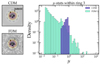 |
Fig. 2. Illustration of the methodology employed in this work. Upper left: Zoom-in of the central halo region magnification map. The dot-dashed white line shows the position of the radial CC, where maximum magnification is achieved (alongside the tangential CC, not shown here). Bottom left: As in the upper left panel, but for the FDM case with a soliton structure at the centre, which further demagnifies the central region, along with wave-like mass density fluctuations that are both positive and negative. Negative fluctuations (δκ < 0) create islands of high magnification inside the CCs, whereas adding more mass (δκ > 0), both in FDM and in CDM, produces the opposite effect and increases demagnification. In both cases, the coloured rings show isomagnification contours (defined in the symmetric CDM case as the CC shape and scaled down by a factor r/rCC) inside the radial CC. These contours enclose regions where we collect magnification statistics of the simulated pixels within each curve for later comparison. Right: Example magnification statistics. Both histograms show the magnification of pixels within the third ring (dark pink) of the left panels. The purple histogram shows the CDM prediction, where μ ≲ 1, as expected for an NFW profile. Ligh blue bins represent the FDM prediction, where both the positive and negative fluctuations in δκ reduce and enhance the magnification compared to CDM. This results in a high probability of both demagnified and highly magnified images. These simulations correspond to a perfectly symmetrical lens (e = 0), a halo mass of M200 = Mh = 7 × 10¹¹ M⊙, and an axion mass of mψ = 10−22 eV. |
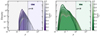 |
Fig. 3. Probability of magnification estimated within smooth CDM isomagnification contours for the CDM profile (left) and corresponding FDM simulations (right). Brighter colours represent larger contours, with the outermost matching the radial CC, while darker colours correspond to smaller contours closer to the centre of the halo. The dashed black vertical line marks a magnification value of ten, which we set as the threshold for comparing p-values. |
5. Results
In this section, we present the main results from the analysis of magnification distributions within radial CCs in FDM-simulated lenses (see Fig. 4) and compare them with those of their CDM counterparts. We also examine the impact of ellipticity in both scenarios and, finally, explore the effects of adding NFW subhaloes to the CDM model compared to the FDM case. For reference, the magnification maps corresponding to the lens models listed in Table 1 are shown in Appendix A.
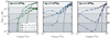 |
Fig. 4. p-values for a magnification factor equal to or larger than ten for each of the simulated lenses. The left panel shows the p-values for the lightest halo mass (3 × 10¹¹ M⊙) for all axion masses. Middle and right panels show the equivalent p-values for the 7 × 10¹¹ M⊙ and 4 × 10¹² M⊙ haloes, respectively. The grey lines represent the complementary p-values for the CDM model at each halo mass. Halo masses increase from left to right with green, blue, and purple colours. The squares, circles, and triangles represent different axion masses, increasing in this order. Dashed, horizontal lines indicate the significance of finding an image with magnification equal to or greater than ten for each model. For the smooth model, it is virtually impossible to achieve such magnification at a distance to the centre of the halo equal to half that of the CC. |
The key distinguishing feature of FDM (and ψDM in general), compared to other dark matter models, is that destructive interferences give rise to negative density fluctuations with respect to the NFW baseline, which in turn generate high-magnification regions inside the CCs (see Fig. 5). Within these curves, the critical condition is fulfilled:1 − κ − γ ≈ 0 for tangential CCs, and 1 − κ + γ ≈ 0 for radial CCs. Adding mass in the form of small-scale perturbers could modify the local magnification distribution; however, on average, it does not significantly affect the global statistics, except for small background sources located close to the perturbers, where the local PDF can change substantially. In contrast, the wave-like fluctuations inherent to FDM can produce extended high-magnification regions, provided that the associated de Broglie wavelength is sufficiently large relative to the lensing scale. These regions are intrinsically different from those produced by CDM subhaloes or other small-scale structures. In the regime where the fluctuation scale is much smaller than the scale of the lens, given by its Einstein radius (such as in galaxy clusters), FDM behaves effectively as a population of millilenses (Diego et al. 2024; Perera et al. 2025).
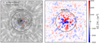 |
Fig. 5. Magnification patterns inside the radial CC (left) and mass density fluctuations (right). Open blue circles mark the positions of negative mass density fluctuations, while open red circles indicate positive fluctuations. Positive fluctuations in the mass (both present in CDM and FDM) inside the radial CC lead to demagnification, whereas negative mass fluctuations (exclusive in FDM) can result in new critical regions. As we approach the centre of the halo, the negative fluctuations in FDM can compensate the increase in κ from the underlying NFW + Sérsic, fulfilling again the radial criticality condition, 1 − κ + γ ≈ 0. |
The two main parameters that govern the FDM fluctuations, and thus the changes in magnification statistics, are the halo mass, Mh, and the axion mass, mψ. The de Broglie wavelength scales with both parameters as shown in Eq. (18), where λdB increases as λdB ∝ mψ−1 and λdB ∝ Mh−1/3. This makes the axion mass the most important factor in the growth of the density fluctuation scale. The size of the CCs–or, in other words, the lensing area of influence for strong lensing effects– increases with the halo mass approximately proportional to M.
Models 11 and 21 feature a λdB much larger than the typical lens scale. In such cases, the resulting perturbations in magnification patterns are excessively strong and would likely already have been detected through image position anomalies. Moreover, no Einstein rings would form in these scenarios, and the deviations far exceed existing tensions. Model 12 behaves similarly, although the effects are slightly milder than in models 11 and 21.
Models 13, 22, and 31 show a large effect without completely disrupting the CCs, as occurs in models 11, 21, and 12. These models present a central demagnification caused by the soliton, corresponding to larger halo and axion masses. All of these models exhibit the largest p-values, as shown in Fig. 4.
Models 23 and 32 are similar to each other and show smaller perturbations confined to regions very close to the CCs, resembling the millilensing or microlensing regime. Their p-values also indicate an increased probability of high-magnification regions (μ ≥ 10) near the centre, due to the presence of a secondary CC created by the soliton, at the cost of enhanced demagnification further in.
Finally, model 33 illustrates the regime in which FDM approaches standard CDM within the resolution limits of this study. At this resolution, the only distinction between FDM and CDM is the presence of the solitonic core, which increases the probability of high magnification near the halo centre. At much higher resolution, the small-scale density fluctuations would still be visible and their effects would resemble those of microlenses.
5.1. Ellipticity
In this study, we have considered only axisymmetric lenses up to this point. However, real lenses typically exhibit some degree of ellipticity. This ellipticity ranges from 0, corresponding to perfectly circular profiles, up to approximately e = 0.5, which is considered extremely large, as higher values are rare in nature.
For ellipticity, we adopted three nominal values: 0, 0.2, and 0.4, and repeated the same analysis in each case, studying the magnification distributions within the isomagnification contours inside the radial CC. For simplicity, we restricted ourselves to a single axion mass and halo mass, corresponding to those of model 22. These magnification maps are shown in Fig. 6. We observe a decrease in the area enclosed by the radial CC, which moves progressively closer to the centre of the halo. Initially, the shape stretches along the direction of the minor semi-axis, but at higher ellipticities it also shrinks along that axis. As shown in Fig. 7, for e = 0.2, the p-values are higher than in the circular case. However, at the highest ellipticity, the area of high magnification becomes significantly smaller. Images within the smaller radial CC are more likely to be demagnified; thus, the p-values are smaller than the two other cases. Nevertheless, some regions of high magnification exist between CCs along the minor semi-axis, although these are not covered in this work.
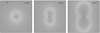 |
Fig. 6. Ellipticity effects on magnification. From left to right, the lens ellipticity increases from none to high. The lens parameters are those of model 22 from Table 1 (Mh = 7 × 10¹¹ M⊙ and mψ = 10−22 eV). The smooth CCs stretch along the major axis and compress along the minor axis, forming an hourglass-shaped configuration. Fluctuations in FDM follow the elliptical mass distribution of the lens; as a result, fluctuations located farther from the centre are attenuated, while those closer in are enhanced. Inside the radial CC, however, as the CC approaches the halo centre, the density fluctuations overlap with the soliton region and are consequently suppressed. In contrast, the interface between the tangential and radial CCs experiences enhanced magnification. The black lines correspond to the CCs of the smooth CDM model. |
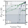 |
Fig. 7. p-values for magnification values equal to or greater than ten in both the smooth CDM model (purple), and the wave-like FDM model (green). Each point represents the p-value calculated for pixels inside the scaled CC contours, with a size expressed as a fraction of the radial CC size (r/rCC). Different marker symbols denote the p-values corresponding to different ellipticity realizations. As in Fig. 4, the p-value is the probability within the given model of attaining a magnification equal to or greater than ten. Dashed, horizontal dashed lines indicate the significance contours. The halo and axion masses correspond to model 22 in Table 1, with Mh = 7 × 10¹¹ M⊙ and mψ = 10−22 eV. |
5.2. CDM subhaloes
The main objective of this paper is to demonstrate that the enhanced magnification statistics observed in the central regions of FDM haloes (containing both negative and positive mass fluctuations relative to the underlying NFW) are difficult to reproduce within classical ΛCDM models, where mass offsets relative to the NFW baseline can only be positive. These enhanced statistics appear to be a unique feature of the negative fluctuations in FDM (or potentially other wave-like dark matter models not considered here). To explore this, we focussed again on halo model 2 (Mh = 7 × 10¹¹ M⊙) and introduced subhaloes at various positions and with different masses inside the region enclosed by the radial CC.
We considered three subhalo masses: 106 M⊙, comparable to the most massive globular clusters; 107 M⊙; and 108 M⊙, representative of low-mass dwarf galaxies. Different subhalo positions were explored to account for the enhanced lensing effect when a lens lies near the CC. In such cases, a point-mass lens of mass M located close to a CC with magnification μ behaves as if it has an effective mass of Meff = μ × M. We modelled subhaloes with axisymmetric NFW profiles, adopting concentration parameters scaling as M−0.1 (Dutton & Macciò 2014) and scale radii scaling as M1/3. We adopted reference values of c = 45.7 and rs = 0.18 kpc for a 106 M⊙ subhalo, scaling these quantities accordingly for the other masses.
When including subhaloes, we find a slight increase in the magnification p-values (for μ ≥ 10) compared to the smooth CDM case, as shown in Figs. 8 and 9. However, this enhancement is smaller than that produced by FDM (see Fig. 4). Interestingly, when the subhalo is too massive (108 M⊙), it can even reduce the p-values with respect to the base model without subhaloes, when considering a large radius for the contour of the studied region, as illustrated in Fig. 9. This can be understood as an increase in the curvature of the deflection field of the otherwise smooth model. Since magnification is inversely proportional to the curvature of the deflection field, adding more (positive) substructure reduces the magnification. Alternatively, this can be understood as the term μr−1 = 1 − κ + γ deviating further from ≈0 (and becoming more negative) when κ increases inside the radial CC.
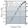 |
Fig. 8. p-values for magnification values equal or greater than ten in the smooth CDM model (purple) and adding a subhalo of 107 M⊙ at different positions relative to the centre of the main halo. As in Figs. 4 and 7, the p-value is the probability of obtaining an image with magnification equal to or greater than ten given the models. The significance values are indicated by the dashed horizontal lines. The halo and axion masses correspond to model 22 in Table 1, with Mh = 7 × 10¹¹ M⊙ and mψ = 10−22 eV. |
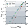 |
Fig. 9. Same as Fig. 8, showing p-values for magnifications equal to or greater than ten in the smooth CDM model and after adding subhaloes. In this case, the subhalo mass varies between realisations, as colour-coded in the legend, while its position is fixed at half the radius of the radial critical curve from the centre of the main halo. The halo and axion masses correspond to model 22 in Table 1, with Mh = 7 × 10¹¹ M⊙ and mψ = 10−22 eV. |
The inclusion of subhaloes induces two distinct effects: (i) they can form small secondary CCs at their positions, resulting in higher μ, but locally reducing magnification near them. However, the p-values in these regions remain low, and highly magnified central images remain statistically rare; (ii) if located near the radial CC and sufficiently massive, a subhalo can distort and pull the main CC inward. Even then, the probability of achieving high magnifications stays below that expected from FDM.
When subhaloes are placed closer to the halo centre, their impact on the global magnification statistics within the radial CC region diminishes, as shown in Fig. 8. In the limit where a subhalo lies exactly at the centre, its behaviour becomes nearly indistinguishable from that of the smooth CDM case. This effect is partially explained by the magnification of the macro model (i.e. the galaxy halo) at the subhalo’s location. Subhaloes near the radial CC, where μ > 1, thus behave as if they were more massive, effectively shifting the radial CC inward and increasing the p-values within the smaller contours near the centre. Conversely, subhaloes located closer to the centre, where μ < 1, behave as if they had lower effective masses. In these cases, any increase in p-values is primarily driven by the formation of secondary CCs, similar to those produced by a solitonic core; however, these secondary CCs can also demagnify the region inside them. Since the central macro magnification is lowest, the enhancement in p-values for centrally placed subhaloes remains minimal.
When the subhalo position is fixed (see Fig. 9), the behaviour simplifies: more massive subhaloes, being stronger overdensities, more effectively demagnify their central region and reduce the higher magnification area. Subhaloes closer to the radial CC remain more efficient at perturbing and shifting the CC inward.
While subhaloes alone cannot reproduce the magnification statistics of FDM, they may still contribute to positional anomalies, similarly to perturbations introduced by small satellite galaxies or low-mass cluster members.
6. Discussion
The results presented in this work highlight a key observational distinction between standard CDM and FDM in the context of strong gravitational lensing: FDM gives rise to a higher probability of magnification within the radial CC as a consequence of interference-driven density patterns. In particular, the negative mass fluctuations in FDM can compensate for the increase in κ inside the radial CC, resulting in new critical regions around the negative fluctuations. Meanwhile, standard CDM models, even when including subhaloes, fail to reproduce similar levels of central magnification. This behaviour, unique to FDM scenarios, offers a promising avenue for constraining the nature of dark matter through precise lensing measurements.
Specifically, we find that extended high-magnification regions near the centre of lenses, associated with soliton-induced secondary CCs and fluctuations on de Broglie scales, are difficult to mimic with conventional CDM substructure. This result suggests that magnification statistics within radial CCs, over a large span of well-modelled lenses, can provide a complementary probe of FDM. With the next generation of surveys, including the ongoing EUCLID mission, the upcoming Rubin-LSST, and Roman, thousands of galaxy-scale lensing systems are expected to be discovered. These systems can then be followed up with specialised instruments that are better suited for strong lensing and/or spectroscopic analysis.
The magnification statistics presented here characterise regions of high magnification but do not capture the spatial distribution of magnifications. Extended sources would require a follow-up analysis incorporating convolved magnification maps with specific source shapes. Nonetheless, point-like sources are better suited to test this statistical framework. Given the resolution of our simulation, we argue that bright, small sources such as quasars (QSOs) are well described by our results and represent an ideal observational test of the predictions presented here. Subparsec, compact but luminous star clusters, which are larger sources, are even more suitable, as they are less affected by microlensing than QSOs.
While some axion mass ranges near 10−22 eV have been excluded by complementary constraints, it has been argued that these limits remain weak due to modelling assumptions or noisy data. Here, we present a complementary lensing-based method to constrain these ranges.
The smallest axion masses (10−23 eV) are unlikely, as the large distortions they produce in the critical curves should already have been observed. The intermediate range, around 10−22–10−21 eV, yields plausible effects. However, we argue that the largest axion mass considered may provide the most compelling case. While smaller axion masses produce deviations from the smooth CDM model that are too strong to have gone unnoticed, this higher mass yields lensing effects that remain significant when applied to lower-mass haloes but consistent with current observational constraints in more massive haloes, where the behaviour closely resembles that of CDM. Interestingly, these smaller haloes are more challenging to detect observationally, suggesting that this axion mass still offers a viable and testable window for future studies.
Some unmodelled effects remain, such as the presence of a central supermassive black hole. We argue that such a component would act as a point-like lens, slightly shifting the smooth CC outwards and introducing a small inner CC, while leaving the main results of this work effectively unchanged. However, its impact on the solitonic structure is less clear and is beyond the scope of this study; therefore, a detailed analysis is deferred to future work. It is also important to note that the true global density profiles of real galaxies remain uncertain. Current models represent the best approximations based on available data and theoretical expectations. Any revision to our understanding of the smooth mass distribution would directly affect the resulting lensing predictions and constraints.
A source of uncertainty arises in the detection of central bright images, due to the difficulty in disentangling them from the emission of the lens galaxy itself. In this regard, spectroscopic follow-up observations would be valuable to distinguish between the two, since complementary images of the lensed source provide an expected spectrum that can be used to separate it from the lens galaxy. The application of this methodology to observational data, along with the associated challenges, will be addressed in future studies. With the advent of new facilities conducting large, deep surveys, we anticipate a wealth of data–particularly for central images of lensed QSOs–that will enable a detailed statistical study of CDM versus FDM.
7. Conclusion
We explored the impact of wave-like dark matter fluctuations on gravitational lensing magnification patterns, with a focus on radial critical curves (CCs). Our analysis reveals observational signatures that distinguish FDM from classical CDM, particularly in compact lensing configurations. The main conclusions of this work are as follows.
-
We have shown that wave-like density fluctuations inherent to FDM can enhance magnification near radial CCs in a manner that is difficult to reproduce with CDM, even when including substructure. In particular, the negative fluctuations in FDM (relative to the NFW profile), which are not present in standard CDM, can produce islands of high magnification in the region interior to the radial critical curve. Such islands cannot be reproduced by classical CDM models.
-
Our results indicate that axion masses in the range 10−22–10−21 eV, especially within low-mass haloes, produce effects distinguishable from CDM and merit further investigation.
-
Statistical differences in magnification, particularly for point-like sources such as QSOs or compact star clusters near the centres of lenses, offer a promising observational signature for constraining ultralight axion dark matter. This work motivates targeted searches for these compact, highly magnified sources within radial arcs as potential probes of the FDM parameter space.
-
While enhanced central images are more probable in the FDM scenario, they remain plausible, though less probable, in standard CDM models with subhaloes. To place robust constraints on the axion mass, a statistically significant sample of lenses with anomalous radial images is required. Each system would necessitate a tailored lens model, given the highly non-linear uncertainties associated with the observational data. A joint likelihood analysis combining multiple systems would strengthen such constraints. Upcoming wide-field surveys, such as Euclid, Rubin-LSST, and Roman are expected to detect numerous lensed systems, providing a promising dataset for pursuing this approach. The number of systems with anomalous radial images required to place a robust constraint on the axion mass within the FDM framework is beyond the scope of this paper, as each system would require a tailored lens model and propagate the highly non-linear uncertainties inherent in the observational data.
Acknowledgments
We sincerely thank Hsi-Yu Schive and Pin-Yu Liao for insightful discussions regarding the soliton–halo relation and galaxy parameters. JMP acknowledges financial support from the Formación de Personal Investigador (FPI) programme, ref. PRE2020-096261, associated with the Spanish Agencia Estatal de Investigación project MDM-2017-0765-20-2. J.M.D. acknowledges the support of project PID2022-138896NB-C51 (MCIU/AEI/MINECO/FEDER, UE) Ministerio de Ciencia, Investigación y Universidades. SKL and JL acknowledge the General Research Fund under grant RGC/GRF 17312122, which is issued by the Research Grants Council of Hong Kong S.A.R. PM and TJB are supported by the Spanish Grant PID2023-149016NB-I00 (MINECO/AEI/FEDER,UE), as well as the Basque government Grant No. IT1628-22. PM also acknowledges financial support from fellowship PIF22/177 (UPV/EHU). We acknowledge Santander Supercomputacion support group at the University of Cantabria who provided access to the supercomputer Altamira Supercomputer at the Institute of Physics of Cantabria (IFCA-CSIC), member of the Spanish Supercomputing Network, for performing simulations. We made use of the following software: Python, NumPy, SciPy, Matplotlib, Astropy, and Powerbox.
References
- Aja, B., Arguedas Cuendis, S., Arregui, I., et al. 2022, JCAP, 2022, 044 [Google Scholar]
- Amruth, A., Broadhurst, T., Lim, J., et al. 2023, Nat. Astron., 7, 736 [NASA ADS] [CrossRef] [Google Scholar]
- Arcadi, G., Dutra, M., Ghosh, P., et al. 2018, Eur. Phys. J. C, 78, 203 [NASA ADS] [CrossRef] [Google Scholar]
- Armengaud, E., Palanque-Delabrouille, N., Yèche, C., Marsh, D. J. E., & Baur, J. 2017, MNRAS, 471, 4606 [NASA ADS] [CrossRef] [Google Scholar]
- Boylan-Kolchin, M., Bullock, J. S., & Kaplinghat, M. 2011, MNRAS, 415, L40 [NASA ADS] [CrossRef] [Google Scholar]
- Boylan-Kolchin, M., Bullock, J. S., & Kaplinghat, M. 2012, MNRAS, 422, 1203 [NASA ADS] [CrossRef] [Google Scholar]
- Broadhurst, T., De Martino, I., Luu, H. N., Smoot, G. F., & Tye, S. H. H. 2020, Phys. Rev. D, 101, 083012 [NASA ADS] [CrossRef] [Google Scholar]
- Broadhurst, T., Li, S. K., Alfred, A., et al. 2025, ApJ, 978, L5 [Google Scholar]
- Brook, C. B., Stinson, G., Gibson, B. K., Wadsley, J., & Quinn, T. 2012, MNRAS, 424, 1275 [CrossRef] [Google Scholar]
- Cardone, V. F. 2004, A&A, 415, 839 [NASA ADS] [CrossRef] [EDP Sciences] [Google Scholar]
- Chiang, B. T., Schive, H.-Y., & Chiueh, T. 2021, Phys. Rev. D, 103, 103019 [NASA ADS] [CrossRef] [Google Scholar]
- Chiang, B. T., Ostriker, J. P., & Schive, H.-Y. 2023, MNRAS, 518, 4045 [Google Scholar]
- Cooley, J. W., & Tukey, J. W. 1965, Math. Comput., 19, 297 [Google Scholar]
- Dalal, N., & Kravtsov, A. 2022, Phys. Rev. D, 106, 063517 [NASA ADS] [CrossRef] [Google Scholar]
- Dalal, N., Bovy, J., Hui, L., & Li, X. 2021, JCAP, 2021, 076 [CrossRef] [Google Scholar]
- Del Popolo, A., & Le Delliou, M. 2017, Galaxies, 5, 17 [Google Scholar]
- Diego, J. M., Li, S. K., Amruth, A., et al. 2024, A&A, 689, A167 [NASA ADS] [CrossRef] [EDP Sciences] [Google Scholar]
- Dutton, A. A., & Macciò, A. V. 2014, MNRAS, 441, 3359 [Google Scholar]
- Eberhardt, A., Liang, Q., & Ferreira, E. G. M. 2024, Phys. Rev. D, submitted [arXiv:2411.18051] [Google Scholar]
- Ferreira, E. G. M. 2021, A&ARv, 29, 7 [NASA ADS] [CrossRef] [Google Scholar]
- Flores, R. A., & Primack, J. R. 1994, ApJ, 427, L1 [NASA ADS] [CrossRef] [Google Scholar]
- Furlanetto, G. d., Della Monica, R., & De Martino, I. 2025, Class. Quant. Grav., 42, 075011 [Google Scholar]
- Gentile, G., Salucci, P., Klein, U., Vergani, D., & Kalberla, P. 2004, MNRAS, 351, 903 [Google Scholar]
- Goldberg, D. M., Chessey, M. K., Harris, W. B., & Richards, G. T. 2010, ApJ, 715, 793 [Google Scholar]
- Guedes, J., Callegari, S., Madau, P., & Mayer, L. 2011, ApJ, 742, 76 [NASA ADS] [CrossRef] [Google Scholar]
- Hartley, P., Jackson, N., Sluse, D., Stacey, H. R., & Vives-Arias, H. 2019, MNRAS, 485, 3009 [Google Scholar]
- Hu, W., Barkana, R., & Gruzinov, A. 2000, Phys. Rev. Lett., 85, 1158 [NASA ADS] [CrossRef] [Google Scholar]
- Hui, L. 2021, Ann. Rev. Astron. Astrophys., 59, 247 [Google Scholar]
- Hui, L., Ostriker, J. P., Tremaine, S., & Witten, E. 2017, Phys. Rev. D, 95, 043541 [NASA ADS] [CrossRef] [Google Scholar]
- Iršič, V., Viel, M., Haehnelt, M. G., Bolton, J. S., & Becker, G. D. 2017, Phys. Rev. Lett., 119, 031302 [CrossRef] [Google Scholar]
- Kawai, H., Oguri, M., Amruth, A., Broadhurst, T., & Lim, J. 2022, ApJ, 925, 61 [NASA ADS] [CrossRef] [Google Scholar]
- Keeton, C. R., Gaudi, B. S., & Petters, A. O. 2003, ApJ, 598, 138 [NASA ADS] [CrossRef] [Google Scholar]
- Klypin, A., Kravtsov, A. V., Valenzuela, O., & Prada, F. 1999, ApJ, 522, 82 [Google Scholar]
- Kobayashi, T., Murgia, R., De Simone, A., Iršič, V., & Viel, M. 2017, Phys. Rev. D, 96, 123514 [NASA ADS] [CrossRef] [Google Scholar]
- Kulkarni, M., & Ostriker, J. P. 2021, MNRAS, 510, 1425 [NASA ADS] [CrossRef] [Google Scholar]
- Laroche, A., Gilman, D., Li, X., Bovy, J., & Du, X. 2022, MNRAS, 517, 1867 [NASA ADS] [CrossRef] [Google Scholar]
- Leung, K. K. H., Ahmed, M., Alarcon, R., et al. 2019, EPJ Web Conf., 219, 02005 [Google Scholar]
- Liao, P.-Y., Su, G.-M., Schive, H.-Y., et al. 2024, Phys. Rev. Lett., accepted [arXiv:2412.09908] [Google Scholar]
- Mazure, A., & Capelato, H. V. 2002, A&A, 383, 384 [NASA ADS] [CrossRef] [EDP Sciences] [Google Scholar]
- McCarthy, I. G., Schaye, J., Font, A. S., et al. 2012, MNRAS, 427, 379 [Google Scholar]
- Mocz, P., Vogelsberger, M., Robles, V. H., et al. 2017, MNRAS, 471, 4559 [Google Scholar]
- Moore, B. 1994, Nature, 370, 629 [NASA ADS] [CrossRef] [Google Scholar]
- Moore, B., Quinn, T., Governato, F., Stadel, J., & Lake, G. 1999, MNRAS, 310, 1147 [NASA ADS] [CrossRef] [Google Scholar]
- Nadler, E. O., Drlica-Wagner, A., Bechtol, K., et al. 2021, Phys. Rev. Lett., 126, 091101 [NASA ADS] [CrossRef] [Google Scholar]
- Navarro, J. F., Frenk, C. S., & White, S. D. M. 1996, ApJ, 462, 563 [Google Scholar]
- Navarro, J. F., Frenk, C. S., & White, S. D. M. 1997, ApJ, 490, 493 [Google Scholar]
- Oh, S.-H., Brook, C., Governato, F., et al. 2011, AJ, 142, 24 [NASA ADS] [CrossRef] [Google Scholar]
- Perera, D., Williams, L. L. R., Liesenborgs, J., et al. 2025, MNRAS, 536, 2690 [Google Scholar]
- Pinetti, E. 2025, ArXiv e-prints [arXiv:2503.11753] [Google Scholar]
- Planck Collaboration VI. 2020, A&A, 641, A6 [NASA ADS] [CrossRef] [EDP Sciences] [Google Scholar]
- Powell, D. M., Vegetti, S., McKean, J. P., et al. 2023, MNRAS, 524, L84 [NASA ADS] [CrossRef] [Google Scholar]
- Robles, V. H., Lora, V., Matos, T., & Sánchez-Salcedo, F. J. 2015, ApJ, 810, 99 [Google Scholar]
- Schaller, M., Frenk, C. S., Bower, R. G., et al. 2015, MNRAS, 451, 1247 [Google Scholar]
- Schive, H.-Y., Liao, M.-H., Woo, T.-P., et al. 2014, Phys. Rev. Lett., 113, 261302 [NASA ADS] [CrossRef] [Google Scholar]
- Schive, H.-Y., Chiueh, T., Broadhurst, T., & Huang, K.-W. 2016, ApJ, 818, 89 [NASA ADS] [CrossRef] [Google Scholar]
- Schive, H.-Y., Chiueh, T., & Broadhurst, T. 2020, Phys. Rev. Lett., 124, 201301 [Google Scholar]
- Schneider, P., Ehlers, J., & Falco, E. E. 1992, Gravitational Lenses (Berlin, Heidelberg: Springer) [Google Scholar]
- Shajib, A. J., Birrer, S., Treu, T., et al. 2019, MNRAS, 483, 5649 [Google Scholar]
- Spingola, C., McKean, J. P., Auger, M. W., et al. 2018, MNRAS, 478, 4816 [NASA ADS] [CrossRef] [Google Scholar]
- Tulin, S., & Yu, H.-B. 2018, Phys. Rep., 730, 1 [Google Scholar]
- Viel, M., Becker, G. D., Bolton, J. S., & Haehnelt, M. G. 2013, Phys. Rev. D, 88, 043502 [NASA ADS] [CrossRef] [Google Scholar]
- Xu, D., Sluse, D., Gao, L., et al. 2015, MNRAS, 447, 3189 [NASA ADS] [CrossRef] [Google Scholar]
- Zhang, D., Ferreira, E. G. M., Obata, I., & Namikawa, T. 2024, Phys. Rev. D, 110, 103525 [Google Scholar]
Appendix A: Simulated lenses
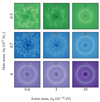 |
Fig. A.1. Magnification maps of simulated lenses according to Table 1. Axion mass increases from left to right, and halo mass increases from top to bottom. |
Appendix B: Image position anomalies
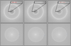 |
Fig. B.1. Radial image configurations for three lens models: a smooth particle-like CDM model (left panel), the same model with a 107 M⊙ subhalo placed halfway between the centre and the radial CC (central panel), and an FDM model corresponding to an axion mass of 5 × 10⁻²² eV (right panel). The top row shows the CCs, while the bottom row shows the corresponding caustics. The blue dots in the bottom panels represent a Gaussian source with a width of 0.8 pixels, placed at the radial caustic to produce bright radial images on the CC. The resulting arcs or images appear in red in the top panels. In the smooth CDM case, the arcs are symmetric and located on top of the radial CC. When a subhalo is added, a similar configuration arises, though the image appears closer to the centre and with lower magnification. In the FDM case, the arcs are asymmetric and exhibit magnification fluctuations on the scale of the axion’s de Broglie wavelength. The two merged radial images seen in the CDM case are now split into distinct components by the fluctuations. Although the caustics are broader in this case, we can confidently say that for an FDM lens, if the source size is comparable to the de Broglie scale, significant image position asymmetries and brighter images closer to the centre can arise compared to the particle-CDM model. |
All Tables
All Figures
|
Fig. 1. Radial profile of an FDM halo (Mh = 7 × 10¹¹ M⊙ and mψ = 10−22 eV at z = 0.9), neglecting quantum fluctuations (solid black line). The inner profile of the halo is dominated by the soliton structure (dot-dashed red line). At r = rsol, the profile transitions to a standard NFW dark matter halo (dashed blue line). The radial variance of the fluctuations, given by Eq. (21) (dot-dashed grey line) is shown in arbitrary units. |
| In the text | |
|
Fig. 2. Illustration of the methodology employed in this work. Upper left: Zoom-in of the central halo region magnification map. The dot-dashed white line shows the position of the radial CC, where maximum magnification is achieved (alongside the tangential CC, not shown here). Bottom left: As in the upper left panel, but for the FDM case with a soliton structure at the centre, which further demagnifies the central region, along with wave-like mass density fluctuations that are both positive and negative. Negative fluctuations (δκ < 0) create islands of high magnification inside the CCs, whereas adding more mass (δκ > 0), both in FDM and in CDM, produces the opposite effect and increases demagnification. In both cases, the coloured rings show isomagnification contours (defined in the symmetric CDM case as the CC shape and scaled down by a factor r/rCC) inside the radial CC. These contours enclose regions where we collect magnification statistics of the simulated pixels within each curve for later comparison. Right: Example magnification statistics. Both histograms show the magnification of pixels within the third ring (dark pink) of the left panels. The purple histogram shows the CDM prediction, where μ ≲ 1, as expected for an NFW profile. Ligh blue bins represent the FDM prediction, where both the positive and negative fluctuations in δκ reduce and enhance the magnification compared to CDM. This results in a high probability of both demagnified and highly magnified images. These simulations correspond to a perfectly symmetrical lens (e = 0), a halo mass of M200 = Mh = 7 × 10¹¹ M⊙, and an axion mass of mψ = 10−22 eV. |
| In the text | |
|
Fig. 3. Probability of magnification estimated within smooth CDM isomagnification contours for the CDM profile (left) and corresponding FDM simulations (right). Brighter colours represent larger contours, with the outermost matching the radial CC, while darker colours correspond to smaller contours closer to the centre of the halo. The dashed black vertical line marks a magnification value of ten, which we set as the threshold for comparing p-values. |
| In the text | |
|
Fig. 4. p-values for a magnification factor equal to or larger than ten for each of the simulated lenses. The left panel shows the p-values for the lightest halo mass (3 × 10¹¹ M⊙) for all axion masses. Middle and right panels show the equivalent p-values for the 7 × 10¹¹ M⊙ and 4 × 10¹² M⊙ haloes, respectively. The grey lines represent the complementary p-values for the CDM model at each halo mass. Halo masses increase from left to right with green, blue, and purple colours. The squares, circles, and triangles represent different axion masses, increasing in this order. Dashed, horizontal lines indicate the significance of finding an image with magnification equal to or greater than ten for each model. For the smooth model, it is virtually impossible to achieve such magnification at a distance to the centre of the halo equal to half that of the CC. |
| In the text | |
|
Fig. 5. Magnification patterns inside the radial CC (left) and mass density fluctuations (right). Open blue circles mark the positions of negative mass density fluctuations, while open red circles indicate positive fluctuations. Positive fluctuations in the mass (both present in CDM and FDM) inside the radial CC lead to demagnification, whereas negative mass fluctuations (exclusive in FDM) can result in new critical regions. As we approach the centre of the halo, the negative fluctuations in FDM can compensate the increase in κ from the underlying NFW + Sérsic, fulfilling again the radial criticality condition, 1 − κ + γ ≈ 0. |
| In the text | |
|
Fig. 6. Ellipticity effects on magnification. From left to right, the lens ellipticity increases from none to high. The lens parameters are those of model 22 from Table 1 (Mh = 7 × 10¹¹ M⊙ and mψ = 10−22 eV). The smooth CCs stretch along the major axis and compress along the minor axis, forming an hourglass-shaped configuration. Fluctuations in FDM follow the elliptical mass distribution of the lens; as a result, fluctuations located farther from the centre are attenuated, while those closer in are enhanced. Inside the radial CC, however, as the CC approaches the halo centre, the density fluctuations overlap with the soliton region and are consequently suppressed. In contrast, the interface between the tangential and radial CCs experiences enhanced magnification. The black lines correspond to the CCs of the smooth CDM model. |
| In the text | |
|
Fig. 7. p-values for magnification values equal to or greater than ten in both the smooth CDM model (purple), and the wave-like FDM model (green). Each point represents the p-value calculated for pixels inside the scaled CC contours, with a size expressed as a fraction of the radial CC size (r/rCC). Different marker symbols denote the p-values corresponding to different ellipticity realizations. As in Fig. 4, the p-value is the probability within the given model of attaining a magnification equal to or greater than ten. Dashed, horizontal dashed lines indicate the significance contours. The halo and axion masses correspond to model 22 in Table 1, with Mh = 7 × 10¹¹ M⊙ and mψ = 10−22 eV. |
| In the text | |
|
Fig. 8. p-values for magnification values equal or greater than ten in the smooth CDM model (purple) and adding a subhalo of 107 M⊙ at different positions relative to the centre of the main halo. As in Figs. 4 and 7, the p-value is the probability of obtaining an image with magnification equal to or greater than ten given the models. The significance values are indicated by the dashed horizontal lines. The halo and axion masses correspond to model 22 in Table 1, with Mh = 7 × 10¹¹ M⊙ and mψ = 10−22 eV. |
| In the text | |
|
Fig. 9. Same as Fig. 8, showing p-values for magnifications equal to or greater than ten in the smooth CDM model and after adding subhaloes. In this case, the subhalo mass varies between realisations, as colour-coded in the legend, while its position is fixed at half the radius of the radial critical curve from the centre of the main halo. The halo and axion masses correspond to model 22 in Table 1, with Mh = 7 × 10¹¹ M⊙ and mψ = 10−22 eV. |
| In the text | |
|
Fig. A.1. Magnification maps of simulated lenses according to Table 1. Axion mass increases from left to right, and halo mass increases from top to bottom. |
| In the text | |
|
Fig. B.1. Radial image configurations for three lens models: a smooth particle-like CDM model (left panel), the same model with a 107 M⊙ subhalo placed halfway between the centre and the radial CC (central panel), and an FDM model corresponding to an axion mass of 5 × 10⁻²² eV (right panel). The top row shows the CCs, while the bottom row shows the corresponding caustics. The blue dots in the bottom panels represent a Gaussian source with a width of 0.8 pixels, placed at the radial caustic to produce bright radial images on the CC. The resulting arcs or images appear in red in the top panels. In the smooth CDM case, the arcs are symmetric and located on top of the radial CC. When a subhalo is added, a similar configuration arises, though the image appears closer to the centre and with lower magnification. In the FDM case, the arcs are asymmetric and exhibit magnification fluctuations on the scale of the axion’s de Broglie wavelength. The two merged radial images seen in the CDM case are now split into distinct components by the fluctuations. Although the caustics are broader in this case, we can confidently say that for an FDM lens, if the source size is comparable to the de Broglie scale, significant image position asymmetries and brighter images closer to the centre can arise compared to the particle-CDM model. |
| In the text | |
Current usage metrics show cumulative count of Article Views (full-text article views including HTML views, PDF and ePub downloads, according to the available data) and Abstracts Views on Vision4Press platform.
Data correspond to usage on the plateform after 2015. The current usage metrics is available 48-96 hours after online publication and is updated daily on week days.
Initial download of the metrics may take a while.