| Issue |
A&A
Volume 701, September 2025
|
|
|---|---|---|
| Article Number | A130 | |
| Number of page(s) | 12 | |
| Section | The Sun and the Heliosphere | |
| DOI | https://doi.org/10.1051/0004-6361/202555813 | |
| Published online | 05 September 2025 | |
Two-way coupled particle-in-cell and magnetohydrodynamic simulation of 2D fan-spine reconnection
1
Rosseland Centre for Solar Physics, University of Oslo, P.O. Box 1029 Blindern, NO-0315 Oslo, Norway
2
Institute of Theoretical Astrophysics, University of Oslo, P.O. Box 1029 Blindern, NO-0315 Oslo, Norway
3
Niels Bohr Institute, University of Copenhagen, Jagtvej 155A, 2200 Copenhagen, Denmark
⋆ Corresponding author: This email address is being protected from spambots. You need JavaScript enabled to view it.
Received:
4
June
2025
Accepted:
4
August
2025
Abstract
Context. Magnetic reconnection is a key mechanism for energy release in the solar atmosphere, but its kinetic-scale microphysics remains difficult to model in large-scale solar geometries.
Aims. We investigate whether fully kinetic particle-in-cell (PIC) simulations can be stably and meaningfully embedded within global magnetohydrodynamic (MHD) models of the solar corona using a realistic fan-spine magnetic configuration.
Methods. We employed a two-way coupled PIC-MHD scheme implemented in the DISPATCH code framework. The PIC solver is embedded within a reconnecting current sheet in a solar-like topology. A physical adjustment of constants is used to bridge kinetic and fluid scales while maintaining self-consistent plasma ordering.
Results. The system evolves stably over more than 45 000 ion plasma periods, exhibiting clear kinetic signatures such as Hall-driven quadrupolar magnetic fields, a reconnection geometry reminiscent of the Petschek configuration, and supra-thermal particle populations. The reconnection rate in the PIC region remains steady and physically consistent, while coupling artefacts are effectively suppressed by fade-in/fade-out boundary weighting.
Conclusions. Our results demonstrate that fully kinetic reconnection can be embedded in global solar MHD models with physical fidelity and computational efficiency. This hybrid approach offers a practical pathway to multi-scale kinetic modelling in realistic astrophysical environments.
Key words: methods: numerical / Sun: flares
© The Authors 2025
 Open Access article, published by EDP Sciences, under the terms of the Creative Commons Attribution License (https://creativecommons.org/licenses/by/4.0), which permits unrestricted use, distribution, and reproduction in any medium, provided the original work is properly cited.
This article is published in open access under the Subscribe to Open model. This email address is being protected from spambots. You need JavaScript enabled to view it. to support open access publication.
1. Introduction
Capturing both the kinetic processes near magnetic reconnection sites and the global evolution of solar flares remains a significant computational challenge. Reconnection involves sharp gradients, strong particle acceleration, and the development of non-thermal particle distributions, all of which violate the assumptions underlying magnetohydrodynamics (MHD; Zharkova et al. 2011). However, these processes occur within large-scale magnetic structures that govern the broader dynamics of flares.
Conventional MHD models excel at describing the evolution of large-scale magnetic fields and bulk plasma flows (Gudiksen & Nordlund 2005; Gudiksen et al. 2011). However, they are inherently unable to resolve the microphysics of reconnection and associated particle energisation. This shortcoming becomes particularly significant in solar flare environments, where localised energy release induces strong departures from fluid behaviour (Pontin & Priest 2022). In contrast, fully kinetic particle-in-cell (PIC) simulations solve the Vlasov-Maxwell equations directly (Birdsall 1991), allowing for the resolution of kinetic-scale physics. Yet, the extreme scale separation between kinetic and global dynamics makes PIC simulations computationally intractable for full-scale solar flares (Birn & Hesse 2001).
Hybrid PIC-MHD frameworks offer a promising path forwards by combining the strengths of the two approaches (Daldorff et al. 2014; Tóth et al. 2016; Makwana et al. 2017; Gordovskyy et al. 2019). Their application to helio-physical problems has seen growing interest, yet the stable and physically consistent embedding of kinetic solvers within global MHD simulations remains technically demanding. In our previous work (Haahr et al. 2025), we introduced a novel PIC-MHD coupling scheme implemented within the DISPATCH framework (Nordlund et al. 2018). There, we demonstrated that embedded kinetic patches can evolve stably within an MHD background, validated through a suite of idealised tests that confirmed accurate wave propagation and consistent behaviour across the PIC-MHD interface.
Here, we advance that methodology by applying the hybrid PIC-MHD model to a 2D fan-spine magnetic topology-an idealised but solar-relevant configuration previously used in flare studies (Nóbrega-Siverio & Moreno-Insertis 2022; Færder et al. 2024). This setup features a magnetic null point and separatrix surfaces where strong gradients and particle acceleration are expected. Fan-spine topologies are commonly observed in the corona and are associated with compact flares and coronal jets (Chitta et al. 2017; Hou et al. 2019; Yang et al. 2020; Priest & Pontin 2009; Masson et al. 2009; Sun et al. 2013).
To our knowledge, this study is the first application of a self-consistent two-way-coupled PIC-MHD simulation to a solar flare-like magnetic geometry. We assess how embedded kinetic regions influence local reconnection dynamics and evaluate the viability of hybrid models in capturing flare-relevant plasma behaviour. In doing so, we aim to bridge the scale gap between global MHD simulations and localised kinetic physics, enabling physically realistic solar flare modelling.
2. Methods
2.1. Numerical framework
All simulations were conducted using the DISPATCH framework (Nordlund et al. 2018), a high-performance, patch-based infrastructure designed for multi-scale, multi-physics simulations. The computational domain is decomposed into semi-independent patches, each containing 32 × 32 cells, which evolve asynchronously using local time-stepping.
Each patch stores multiple temporal slices to enable high-order interpolation during ghost-zone communication. In PIC patches, the time step is globally constrained by the speed of light, while MHD patches evolve under locally Courant-limited conditions. This architecture enables stable and efficient coupling across spatial and temporal scales.
2.2. Magnetohydrodynamics
The MHD background is evolved using the Bifrost solver (Gudiksen et al. 2011), integrated into the DISPATCH framework. Bifrost solves the resistive MHD equations with hyper-diffusive stabilisation, using a staggered-mesh explicit scheme well suited to the sharp gradients and shocks characteristic of solar conditions. The system of equations solved is
 (1)
(1)
 (2)
(2)
 (3)
(3)
 (4)
(4)
 (5)
(5)
 (6)
(6)
Here, ρ is the mass density, u the velocity, e the internal energy per unit volume, B the magnetic field, E the electric field, J the current density, τ the viscous tress tensor, P the pressure, η the magnetic diffusivity, and Q encapsulates source terms such as radiative losses and thermal conduction. We employed fourth-order staggered derivatives. The gravitational term ρg is neglected in this simulation. Bifrost operates using a ‘code unit system’, in which constants such as c and 4π can be absorbed into the definitions of the variables.
Bifrost employs a split diffusive operator composed of global and local (hyper-diffusive) terms to maintain numerical stability while preserving physical fidelity. This enables spatially adaptive dissipation that concentrates smoothing in regions of large gradients, while minimising diffusion elsewhere in the domain.
At each MHD update, electric fields and current densities are reconstructed for communication with neighbouring PIC patches. The formulation used follows Haahr et al. (2025), and is expressed in a unit-agnostic form as
 (7)
(7)
 (8)
(8)
where ne is the electron number density, derived from the mass density under the assumption of fully ionised hydrogen, and e is the elementary charge. The constants kF and kB depend on the unit system adopted. This version of the generalised Ohm’s law includes only the advective and Hall terms, with resistivity omitted to avoid artificial dissipation at the PIC-MHD boundary. While the MHD solver (Eq. (4)) omits the Hall term entirely, since it governs the global evolution where Hall effects are negligible, Eq. (8) includes it to ensure physical consistency when interfacing with the PIC solver near the reconnection site. This ensures physical consistency across the interface and preserves the integrity of kinetic-scale processes.
2.3. Kinetic region: Particle-in-cell solver
The embedded PIC solver is described in detail by Haahr et al. (2025). It is based on the PhotonPlasma code (Haugbølle et al. 2013) and solves the Vlasov-Maxwell system using macro particles for electrons and protons. Fields are evolved on a staggered Yee lattice (Yee 1966), and particles are advanced using the Vay particle pusher algorithm (Vay 2008). The solver supports both explicit and semi-implicit formulations for field evolution and is fully integrated into DISPATCH, inheriting its communication protocols and update procedures.
In the present simulations, each PIC cell contains 200 particles per species. Fields and current deposition utilise piecewise cubic spline shape functions, which ensure high accuracy in charge and current interpolation. Internal energy is computed using the ‘exact’ method, subtracting bulk kinetic energy from the total. The electromagnetic fields are evolved using fourth-order derivatives, consistent with the MHD solver. Particle sorting is performed every 20 time steps to improve cache locality and deposition performance. No particle resampling is applied. The ‘HL’ unit system is used as described in Haahr et al. (2025).
2.4. PIC-MHD coupling
The coupling scheme follows the approach developed in Haahr et al. (2025). The MHD equations are solved in the background across all refinement levels, and selected regions at the highest resolution are overlaid with PIC patches.
Each PIC patch shares the geometric information (position and resolution) of its MHD ‘parent’ patch. Thus, PIC and MHD solvers use the same spatial resolution in regions where they overlap. All patches evolve asynchronously using a local Courant condition to determine the time step. For PIC patches, the Courant condition is limited by the speed of light and is fixed for all PIC patches. For MHD, the local Courant condition can vary between patches. Due to this asynchronous evolution, PIC and MHD patches exchange information at different times.
MHD patches generally take larger time steps than PIC patches. To accommodate this, communication is structured such that MHD patches are influenced by PIC in the ‘pre-update’ phase, while PIC patches receive MHD input in the ‘post-update’ phase. For ‘inner patches’ (MHD patches completely surrounded by PIC patches) the MHD variables (mass density, momentum, internal energy, and magnetic field) are fully overwritten by the corresponding PIC solution after each update. Inner PIC patches are not influenced by MHD.
Patches adjacent to non-PIC zones are classified as ‘transition patches’. In these transition patches, field values are blended using asymmetric weighting to ensure a smooth interface between solvers. Specifically, PIC contributions are gradually introduced over half a patch width within MHD patches and conversely fade out within PIC patches. This method effectively suppresses numerical artefacts and maintains consistency across the PIC-MHD boundary.
2.5. Simulation overview
We simulated a 2D fan-spine magnetic topology inspired by Færder et al. (2024). The initial magnetic field is given by
 (9)
(9)
 (10)
(10)
where B1 = 10/4π G1, k = π/16 Mm−1, and B0 = 0.3B1. The mass density and temperature are initially uniform, with ρ0 = 3 × 10⁻¹⁶ g cm−3 and T0 = 0.61 MK, representative of typical coronal conditions. This corresponds to β = 0.0073, based on B1, T0, and ρ0. The full simulation domain spans 32 × 32 Mm2. The system is energised by a horizontal velocity driver imposed in the lower ghost zones:
 (11)
(11)
where the spatial profile is defined as
 (12)
(12)
and the temporal modulation is given by
![Mathematical equation: $$ \begin{aligned} v_d(t) = {\left\{ \begin{array}{ll} \sin (0.5\pi t / t_r),&t \le t_r, \\ 1,&t_r < t \le t_\mathrm{end} - t_r, \\ \sin [0.5\pi (t_\mathrm{end} - t) / t_r],&t > t_\mathrm{end} - t_r, \end{array}\right.} \end{aligned} $$](/articles/aa/full_html/2025/09/aa55813-25/aa55813-25-eq13.gif) (13)
(13)
with tr = 10 min and tend = 40 min.
Absorbing boundary conditions are applied in the top and bottom 1 Mm of the domain. At the top boundary, all variables are damped, while at the bottom, only mass density, internal energy, and vertical velocity are affected. The system is first evolved for 40 minutes of physical time on a uniform grid of 2048 × 2048 cells. This base simulation is used to initialise refined runs.
2.6. Refinement and PIC region
To resolve kinetic scales, we restarted the simulation from a snapshot at t = 16 min 40 s, a time when the current sheet is fully developed and free from plasmoids. We first applied two levels of refinement: the first spans (13.0, 3.0)–(20.0, 10.0) Mm and the second (14.5, 4.5)–(17.5, 7.5) Mm, resulting in an effective resolution of 8192 × 8192 in the innermost region. The refined areas are illustrated in Fig. 1. Additional high-cadence experiments are performed at both base (2K) and refined (8K) resolutions to capture rapid transient behaviour.
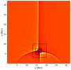 |
Fig. 1. Mass density at the initial refinement time (16 min 40 s). The dotted and solid black squares indicate the first and second refinement levels, respectively. The blue square outlines the PIC region enclosing the current sheet. |
To reduce computational cost while preserving key kinetic features, we applied a physical adjustment of constants (PAC) as outlined in Haahr et al. (2025). Specifically, the vacuum permittivity ϵ0 is reduced by a factor of 100, lowering the effective speed of light by a factor of 10. The PIC runs further vary the electron mass and charge scaling. An overview is provided in Table 1. In the MHD simulations, the current sheet collapses until reaching a width of approximately 2–4 cells, independent of resolution. This scale is set by the effective numerical resistivity. The charge scaling was chosen such that the ion skin depth roughly becomes comparable the current sheet width in the 2K MHD run.
PAC and key scale parameters for each PIC run.
We examined both a ‘big’ (b_) PIC region covering (15.4, 17.1)–(5.3, 7.0) Mm and smaller (s_) regions selected dynamically based on proximity (< 0.2 Mm) to the current sheet, as shown in Figs. 2 and 3. The pure-MHD runs are stable, but in the more physical PAC regimes, several simulations exhibit numerical instabilities due to under-resolved electron-scale structures. In the s_r2_e0_m25 case, the grid resolves the ion skin depth with approximately ten cells and the electron skin depth with about two cells, while the Debye length spans roughly 1/47 of a cell and the electron gyro radius about 1/13 of a cell. This simulation remains stable for the full 50,s runtime.
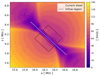 |
Fig. 2. Alfvén velocity in the b_r2_e0_m25 run, 10 s after restart. The dashed region indicates the area used for inflow analysis. The white line traces the current sheet and defines the axis for computing perpendicular velocity components. |
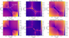 |
Fig. 3. Comparison between the s_r3_e1_m25 PIC run and the high-resolution 8K MHD simulation 35 s after restart. The dashed white outline indicates the PIC region. In the MHD case, a prominent plasmoid is visible in both the density and velocity fields. |
Increasing the mass ratio by a factor of 4 reduces both the electron skin depth and gyro radius by a factor of 2. Similarly, increasing the elementary charge scaling (s_r2_e1_m25) under-resolves all electron scales by an additional factor of 2. These effects destabilise the simulation: the s_r2_e1_m25 run becomes unstable shortly after the ejection of the initial plasmoid, while s_r2_e0_m100 remains stable for most of its runtime but exhibits numerical instability towards the end. The fact that s_r2_e0_m100 is more stable than s_r2_e1_m25 suggests that the Debye length is the most critical limiting factor. These instabilities arise due to internal PIC resolution limits, not from the PIC–MHD coupling itself.
Since both of these PAC scaling changes cause the relevant electron and ion scales to decrease by roughly a factor of two, we compensated for this by introducing a third level of refinement. In the experiments s_r3_e1_m25 and s_r3_e0_m100, this additional resolution restores the resolved electron scales to levels comparable with those in the stable s_r2_e0_m25 run.
2.7. Current sheet geometry
Characterising the current sheet geometry allows us to identify the inflow region used to estimate the reconnection rate (Sect. 2.8), and to quantify the current sheet aspect ratio L/W, a key parameter for assessing susceptibility to tearing instability.
To characterise the geometry of the current sheet in the PIC-coupled simulations, we measured both its length and width. The length of the current sheet was determined from the out-of-plane current density, Jy, sampled along the sheet’s axis. To suppress small-scale fluctuations, a running average was applied to the profile. From the smoothed distribution, we identified the peak value, Jmax, and defined the current sheet boundaries as the points where the current density dropped below 0.7 Jmax on both sides of the current sheet. This threshold was selected to robustly identify the extent of the main reconnection layer while excluding side lobes and numerical noise. The midpoint between these two endpoints was taken as the centre of the sheet.
To estimate the width, we analysed the component of the magnetic field parallel to the sheet, sampled along the direction perpendicular to the sheet’s axis at its centre. The reversal point, where the magnitude of the magnetic field approached zero, was first identified. We then traced outwards in both directions until the absolute value of the magnetic field exceeded 0.4 Bmax, where Bmax is the maximum field strength on either side of the sheet. The total distance between these two points was taken as the full width of the current sheet.
This procedure was applied to all simulation runs. For each run, measurements were averaged over the interval from t = 15 s to t = 34 s. The start time was chosen to avoid initial transients and to ensure that the primary plasmoid had been ejected, marking the onset of a quasi-steady reconnection phase. The end time was selected to precede the onset of secondary plasmoid formation in run s_r3_e1_m25, ensuring that all measurements reflect the quasi-steady regime.
2.8. Reconnection rate
We quantified magnetic reconnection through the inflow velocity normalised by the local Alfvén speed. The reconnection rate is then given by
 (14)
(14)
where vi is the mean inflow velocity component perpendicular to the current sheet, and vA, i is the corresponding mean Alfvén speed. The mean is calculated within the dashed inflow regions in Fig. 2. Only cells where the velocity vector points inwards, towards the current sheet, are included in the averaging.
3. Results
3.1. PIC-MHD evolution and comparison
We assessed the system’s evolution over a 50 s interval following a restart at t = 16 min 40 s. Figure 3 contrasts the density, total velocity, and magnetic field strength between the s_r3_e1_m25 PIC-embedded run and the 8K MHD simulation at 35 s after restart.
At large scales, both simulations remain consistent with each other, indicating that the coupling preserves global structure. However, near the reconnection site, important differences emerge. The current sheet appears broader in the PIC run, and the outflow velocity is reduced and more spatially extended compared to the MHD run. These deviations highlight the influence of kinetic effects in the PIC region.
To evaluate the influence of the PIC region size, we compared runs with extended (b_r2_e0_m25) and compact (s_r2_e0_m25) coverage of the current sheet. The two simulations yielded quantitatively similar reconnection behaviour, demonstrating that a much smaller, dynamically targeted PIC region suffices, achieving substantial computational savings without sacrificing accuracy.
3.1.1. MHD runs
In the 2K MHD simulation, no additional refinement is applied at restart, allowing the system to evolve smoothly without artificial transients. The current sheet remains thin and rapidly becomes unstable to the tearing instability, producing a dynamic reconnection environment with repeated plasmoid formation and ejection.
By contrast, the 8K MHD run introduces grid refinement at restart, which causes the current sheet to collapse to a thickness of 10–20 km. This triggers a transient shock wave, followed by re-stabilisation and the onset of recurrent plasmoid ejections consistent with fast reconnection at high Lundquist number.
3.1.2. PIC run
The PIC-embedded simulation initially mirrors the 8K MHD evolution. The current sheet collapses and launches a shock wave, followed by the ejection of a single plasmoid. However, after this transient, the system stabilises into a broadened current sheet that persists throughout the remainder of the run.
A quadrupolar structure emerges in the out-of-plane magnetic field component (By), as illustrated in Fig. 4. This is a characteristic signature of Hall-scale reconnection and is entirely absent in the pure MHD simulations. In our coupled setup, the structure is generated within the PIC region and, upon reaching the PIC–MHD boundary, is advected along the separatrices into the surrounding MHD domain. The signature remains visible along the separatrices far from the PIC region, demonstrating the coupling scheme’s ability to communicate physical features, such as Hall effects, that are inaccessible to MHD alone, into the global system.
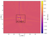 |
Fig. 4. Out-of-plane magnetic field component (By) in the b_r2_e0_m25 PIC simulation, 30 s after restart. A quadrupolar Hall signature emerges within and beyond the PIC domain. |
The transition across the PIC-MHD boundary remains smooth, with minimal artefacts. While high-frequency noise from particle discreteness is visible-especially in the velocity field–the fade-in/fade-out coupling scheme ensures that such disturbances remain localised.
3.2. Influence of PAC parameters
Figure 5 presents the thermal energy density 6 s after restart for a subset of PIC runs, and Fig. 6 shows the evolution after 15 s. All configurations show the formation of a single plasmoid. This is followed by the development of a broadened, quasi-steady current sheet. While this overall evolution is robust across runs, the morphology of the sheet and plasmoid is sensitive to the chosen PAC parameters.
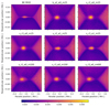 |
Fig. 5. Thermal energy density (in erg cm−3) for selected PIC runs, shown 6 s after restart. All simulations display a single ejected plasmoid in the process of formation. PAC parameters influence the plasmoid morphology. The 8K MHD case is shown for reference. |
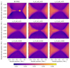 |
Fig. 6. Thermal energy density (in erg cm−3) for selected PIC runs, shown 15 s after restart. PAC parameters influence the current sheet width and shape. The 8K MHD case is shown for reference. The s_r2_e1_m25 run experiences numerical instability, which is visible below the current sheet in the sub-figure. |
More extreme PAC settings (e.g. e0_m25) produce diffuse current sheets with poorly defined boundaries, whereas milder PAC adjustments or higher spatial resolution yield sharper, more collimated structures. Simulations with elevated proton-to-electron mass ratios (m100 and m400) exhibit a more complex internal plasmoid structure, featuring compact, hot, and dense cores embedded within broader, diffuse halos.
Despite these morphological differences, all simulations evolve towards a reconnection geometry reminiscent of the Petschek configuration–i.e. a compact diffusion region and open outflow jets–after the initial plasmoid is expelled. The principal effect of PAC tuning is on the geometry of the current sheet, as quantified in Table 2. Based on the initial density ρ0, the ion skin depth is approximately 35 km for e0 runs and 18 km for e1 runs. The current sheet length, when normalised by the ion skin depth, varies significantly across the different PAC configurations. In contrast, for simulations with the same electron mass, the current sheet width remains approximately constant in units of di, even when the elementary charge is increased and the ion skin depth is halved. The sheet becomes systematically thinner for higher ion-to-electron mass ratios, corresponding to a reduced and more realistic electron skin depth. The resolution and PIC domain size have a relatively minor influence on these trends; rather, the observed variations are driven primarily by the PAC parameters.
Current sheet geometry for PIC runs.
Increasing the proton-to-electron mass ratio (e.g. s_r3_e0_m400) leads to a marked reduction in current sheet length. The L/di scale roughly as  . The width is also reduced for higher mass ratios, but does not exhibit the same
  dependence. Compared to the length, the width remains comparatively stable, collapsing the structure into a compact, localised X-point. Conversely, reducing the elementary charge scaling (e.g. s_r3_e1_m25) produces the thinnest current sheets, with the highest aspect ratio observed.
These differences in geometry strongly influence the onset of secondary tearing. The tearing mode is suppressed in short, thick sheets, where the low aspect ratio stabilises the current layer. In contrast, the elongated sheet in the most realistic configuration, s_r3_e1_m25, becomes unstable around t = 35 s and ejects a secondary plasmoid, as shown in Fig. 7. This is the only PIC run where secondary tearing is observed, highlighting the sensitivity of instability onset to PAC-controlled aspect ratio.
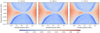 |
Fig. 7. Secondary plasmoid formation in the s_r3_e1_m25 simulation, shown as relative density compared to ρ0. The event occurs around 35 s after restart, within the elongated current sheet produced by this PAC configuration. |
3.3. Reconnection rate
Figure 8 shows the time evolution of the normalised reconnection rate for the primary MHD and PIC runs. Both MHD simulations exhibit pronounced temporal variability, characterised by bursts associated with plasmoid formation and ejection. The 8K run, in particular, features sharp peaks, consistent with fast, impulsive reconnection at high Lundquist number. In contrast, all PIC simulations transition into a steady-state reconnection regime shortly after the initial plasmoid is ejected. The reconnection rate stabilises near 0.05–0.06 and remains largely constant throughout the remainder of the simulation, with no further bursts or instabilities observed.
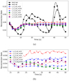 |
Fig. 8. Normalised reconnection rate evolution. Panel (a): Time evolution of the normalised reconnection rate for the 2K and 8K MHD simulations and selected PIC runs. Panel (b): Zoom-in on the PIC runs between t = 15 and 50 s (after the ejection of the initial plasmoid), showing the more stable reconnection rate after the initial collapse. |
Across the PAC parameter survey, systematic trends emerge. Runs with higher proton-to-electron mass ratio and weaker charge scaling (i.e. a higher elementary charge) exhibit slightly elevated reconnection rates, in agreement with our earlier findings (Haahr et al. 2025). Conversely, increasing spatial resolution appears to result in a modest decrease in reconnection rate. We also examined the magnetic field in the vicinity of the current sheet to investigate this further. We show the evolution of the square of the magnetic field strength perpendicular to the current sheet for run s_r3_e1_m1 in Fig. 9. The figure shows an initial collapse (which also triggers the initial ejection of a plasmoid). As shown in the integrated field, this collapse is also associated with a significant drop in magnetic flux near the current sheet. The current sheet then stabilises, and magnetic flux slowly accumulates again. Around t = 35 s, a critical point is reached, the current sheet becomes unstable, and a smaller secondary plasmoid is ejected, followed by another drop in the integrated field strength. The current sheet again becomes unstable around t = 48 s, and another small plasmoid is ejected, followed by a drop in integrated field strength.
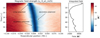 |
Fig. 9. Evolution of the magnetic field square along the current sheet’s perpendicular axis. The figure shows the initial collapse of the current sheet, which is associated with the ejection of a plasmoid. We then observe a stable period with slow accumulation of magnetic flux, during which two secondary plasmoids are also ejected, resulting in drops in the integrated field strength. |
We then compared the integrated field strength for all stable runs (see Fig. 10). The physical setup s_r2_e0_m100 remains stable, but slight numerical instabilities causes oscillatory fluctuations in the integrated field. However, this is not reflected in the reconnection rate for this run. Common for all runs is an initial drop in magnetic field strength during the ejection of the initial plasmoid. After this, all runs reach a quasi-steady state where the magnetic field strength slowly grows.
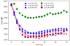 |
Fig. 10. Integrated magnetic field strength along the perpendicular direction at the centre of the current sheet. The values are in code units. |
The comparison in Fig. 10 highlights the most important reason for the different reconnection rate: Magnetic field strength (and by extension the Alfvén velocity in the inflow region) is generally higher for high resolution runs, lower for larger electron-to-proton mass ratio, and much higher for smaller elementary charge scaling. While the integrated field strength differs significantly across PAC runs close to the current sheet, they all converge to the same field strength roughly 0.2 Mm away from the current sheet at the PIC-MHD interface. The lower field strength is thus a direct consequence of the change in geometry, as they all share the same magnetic field strength far from the current sheet, a broader width will result in a lower aggregated field strength.
While these trends are systematic, their overall effect on the reconnection rates is small, and the parameter space sampling remains sparse, with only two data points per parameter direction (mass ratio, charge scaling, and resolution). Consequently, the statistical significance of these trends is limited. Nonetheless, the results suggest that the reconnection rate in this hybrid PIC-MHD setup is relatively robust to moderate variations in kinetic scaling.
3.4. Particle energy spectra
We concluded by examining the particle energy distributions within the current sheet. To isolate the core reconnection region and exclude inflow and outflow effects, we selected all particles located within 0.15 Mm along and 0.02 Mm across the current sheet measured from the centre of the current sheet.
At each time step, we fitted Maxwell-Boltzmann distributions to the empirical energy probability density functions for both electrons and protons. We present here the findings in our most realistic PAC run, s_r3_e1_m25. Here, the electron temperature decreases from 0.6 MK to 0.48 MK over the first 20 s and then remains approximately steady. In contrast, the proton temperature declines more gradually, from 0.61 MK to 0.54 MK by the end of the simulation. This disparity indicates that electrons rapidly attain a quasi-equilibrium state, while protons thermalise on longer timescales, consistent with their greater inertia and slower collisional coupling. This drop in current sheet temperature is not a sign of cooling in the thermodynamic sense, but reflects a structural transition: the system adjusts from a narrow and hot MHD-derived current sheet to a broader, cooler, and PIC-resolved equilibrium.
As shown in Fig. 11, both particle species develop increasingly pronounced deviations from a Maxwellian distribution over time, manifesting as supra-thermal tails. Such non-thermal features are a well-known result of magnetic reconnection, reported in both PIC (Drake et al. 2006; Egedal et al. 2010; Baumann et al. 2013; Guo et al. 2014; Dahlin et al. 2017; Arnold et al. 2021) and test-particle (Dalena et al. 2014; Gordovskyy et al. 2019; Zharkova et al. 2011) simulations. Although some studies have explored proton acceleration (e.g. Seo et al. 2024), the majority focus on electron energisation. In contrast, our results show that the most prominent supra-thermal features emerge in the proton distributions, which steadily accumulate high-energy particles over time. Electron distributions exhibit greater temporal variability but also display a gradual enhancement of their high-energy tails.
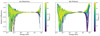 |
Fig. 11. Relative difference between the particle energy probability density function and the best-fit Boltzmann distribution over time for electrons (left) and protons (right). Both species develop supra-thermal tails as the simulation progresses, particularly protons. |
The fraction of particles with energies exceeding 100 keV and lying above the best-fit Maxwellian-that is, the non-thermal excess–is approximately 10−4 for electrons and 4 × 10⁻⁴ for protons. These supra-thermal particles represent a persistent high-energy component that is not accounted for by thermal heating alone. When including both the thermal and non-thermal contributions, the total number density of > 100 keV particles reaches approximately 1.0 × 106 cm−3 for electrons and 1.3 × 106 cm−3 for protons.
4. Discussion
4.1. Evolution of the current sheet
While both MHD runs exhibit repeated plasmoid formation consistent with the tearing instability (Bhattacharjee et al. 2009), the PIC simulation evolves differently. After ejecting a single plasmoid during the initial current sheet collapse, it enters a stable reconnection regime with no further tearing, except in one case. Several interrelated factors likely contribute to this suppression.
First, PAC modifies plasma scales, yielding a broader current sheet than in the MHD cases, even wtih minimal scaling. Since plasmoids must exceed the sheet width to form, this broadening raises the instability threshold. A small secondary plasmoid is observed in the most realistic PAC configuration (s_r3_e1_m25), which produces the current sheet with the largest length-to-width ratio among the PIC runs, underscoring the critical role of PAC in determining sheet stability. For less realistic PAC configurations (e.g. s_r3_e0_m25), where the current sheet is broader, plasmoids of comparable size would remain embedded in the sheet structure and thus be indistinguishable from the background current sheet. Second, the PIC simulations develop a quadrupolar out-of-plane magnetic field, characteristic of Hall-type reconnection (Uzdensky & Kulsrud 2006). Third, the reconnection driving mechanism is Hall-based, with the reconnection geometry resembles a Petschek-like configuration, with a compact diffusion region and collimated outflows. This setup naturally supports steady, fast reconnection without requiring plasmoid mediation. In contrast, the MHD simulations a driven by resistive reconnection and form elongated Sweet-Parker-like sheets that are more prone to fragmentation.
Similar conclusions have been drawn in previous fully kinetic studies. For instance, Daughton et al. (2006) investigated a range of idealised reconnection setups and found that the formation of secondary plasmoids is highly sensitive to the choice of PAC parameters. Our results support these findings: only the most realistic PAC configuration, which achieves the highest aspect ratio, exhibits secondary tearing. They further emphasised that while plasmoid formation is generally associated with the tearing mode instability, the onset conditions differ in kinetic regimes due to the altered structure of the electron diffusion region.
4.2. Resolution and plasma scales
Capturing plasma dynamics in kinetic simulations requires resolving key microphysical scales, particularly the Debye length, ion and electron skin depths, and gyro radii. These scales depend on local plasma conditions and are influenced by the PAC applied in our setup.
For the most pronounced PAC modifications (e0_m25), the initial Debye length is approximately 80 m, while the ion skin depth is about 34 km at ρ = 3 × 10⁻¹⁶ g cm−3 and T = 0.61 MK. This yields more than 400 Debye lengths per ion skin depth. Our grid resolves the ion skin depth with > 10 cells-adequate for capturing ion-scale reconnection physics. However, the Debye length is under-resolved: there are approximately 47 Debye lengths per grid cell.
Under-resolving the Debye length can, in principle, lead to aliasing instabilities and artificial heating effects, as documented in early kinetic studies (Langdon 1970; Birdsall & Maron 1980). However, Barnes & Chacón (2021) show that in energy-conserving PIC schemes, stability is not strictly tied to Debye length resolution but also depends on the numerical methods used. Our solver incorporates high-order interpolation and derivatives, as well as semi-implicit field updates-all of which help suppress numerical instability effects. Moreover, our PIC-MHD coupling employs a fade-in/fade-out strategy that damps standing waves and spurious reflections at the interface, further enhancing stability even in under-resolved regions.
Despite the scale disparity, our simulations produce physically consistent results. The reconnection geometry, Hall magnetic signatures, and particle energy spectra exhibit the expected behaviour. Minor discrepancies, such as enhanced noise in the high-energy tails of the electron spectra, likely arise from statistical fluctuations and the limited resolution of electron-scale processes. The e0_m25 configuration operates near the edge of numerical stability, whereas more moderate PAC choices (e1_m25, e0_m100, and e0_m400) required finer grid resolution to remain stable. Finally, we note that our fully electromagnetic, relativistic PIC solver is particularly well suited for studying more extreme, higher-temperature reconnection events. As the ratio  , higher temperatures naturally increase the Debye length relative to the ion skin depth, thereby relaxing resolution requirements and expanding the accessible kinetic regime.
4.3. Reconnection rate comparison
The reconnection rate provides a quantitative metric for comparing the dynamical evolution of MHD and PIC simulations. In the MHD runs, strong temporal variability arises from the tearing instability. As secondary plasmoids form and are expelled, inflow is transiently enhanced, producing sharp peaks in the reconnection rate. Between ejections, the rate falls, reflecting the cyclic growth and saturation of tearing modes in elongated current sheets.
The PIC-embedded simulation follows a contrasting path. After ejecting a single plasmoid during the initial collapse, it transitions to a stable regime with a nearly constant reconnection rate. This behaviour reflects the emergence of a compact diffusion region with collimated outflows, consistent with Petschek-type fast reconnection. The absence of further tearing removes the primary driver of variability, resulting in steady and continuous energy conversion.
A key distinction in the PIC case is the emergence of a quadrupolar out-of-plane magnetic field, characteristic of Hall-type reconnection. This component can also act as a weak guide field, helping magnetise particles in the diffusion region. For stronger guide fields, prior studies have shown stabilisation of the current sheet and a reduction in reconnection rate (Drake et al. 2006; Chen et al. 2017).
The use of PAC-essential for embedding kinetic regions in large-scale environments-also influences the absolute reconnection rate. Previous work on simplified setups (Haahr et al. 2025) showed that PAC typically leads to a modest suppression of the rate, even when global geometry and skin-depth-to-sheet-width ratios are preserved. This suggests PAC alters not just macroscopic structure but also the balance of terms in the generalised Ohm’s law. This mild PAC dependence aligns with findings by Hesse et al. (2018), who show that the reconnection rate is primarily governed by large-scale ion inflow, which is only moderately affected by PAC scaling.
Despite these adjustments, the reconnection rates observed here remain consistent with results from prior collisionless reconnection studies, including the GEM challenge (Pritchett 2001; Otto 2001; Birn & Hesse 2001; Kuznetsova et al. 2001). Achieving physically realistic reconnection rates, with clear Hall signatures and Petschek-like structure, using modest computational resources, underscores the value of our hybrid approach. It enables the study of kinetic reconnection in complex configurations-such as the fan-spine topology used here-without requiring full PIC domain coverage. These results confirm that physically consistent kinetic reconnection can be stably embedded in large-scale simulations using the PAC strategy.
4.4. Particle acceleration
Particle energisation is a key feature of magnetic reconnection and a primary motivation for incorporating kinetic physics into global models. Our PIC-embedded simulations enable the direct tracking of electron and proton energy distributions within the current sheet, offering insights into the efficiency and mechanisms of acceleration in this solar-like configuration.
Both particle species develop mildly non-Maxwellian energy distributions, though the proton spectra consistently exhibit a more prominent high-energy tail. This asymmetry likely arises from their differing inertial and thermalisation properties: electrons, being less massive, quickly respond to local electric field fluctuations, whereas protons gain energy more gradually, resulting in a steady build-up of a supra-thermal component. The number density of particles with energies exceeding 100 keV reaches 1.0 × 106 cm−3 for electrons and 1.3 × 106 cm−3 for protons. Observational estimates place the number density of accelerated electrons in flaring regions at approximately 1010 cm−3 (Fletcher et al. 2011). However, this observational value carries significant uncertainties–particularly in the volume estimation of the flare kernel–and is derived from more turbulent environments, which likely act as more efficient accelerators than those studied here. Taking this into account, our simulation results are in reasonable agreement with observational constraints.
A notable result is that the number of > 100 keV supra-thermal protons exceeds that of supra-thermal electrons. While electron beams have been extensively studied, studies of the effect of accelerated protons are rare, especially for low energies, < ∼MeV. This gap in our knowledge stems from the fact that protons must be accelerated to much higher energies to be observed. As a result, their influence on flare dynamics remains poorly constrained. Our hybrid PIC-MHD framework provides a new pathway for investigating the role of non-thermal protons in energy transport during reconnection.
Despite the presence of supra-thermal tails, the spectra remain only mildly non-thermal. This contrasts with the stronger power-law features found in 3D PIC studies of reconnection (Baumann et al. 2013), where turbulence, magnetic field stochasticity, and flux rope interactions enhance acceleration. Our setup’s relative smoothness and two-dimensionality likely limit the formation of strongly non-thermal populations.
Common particle acceleration mechanisms include Dreicer acceleration (Dreicer 1959), first-order Fermi processes (Drake et al. 2006; Guo et al. 2014), and second-order Fermi acceleration (Dalena et al. 2014). In our setup, the absence of plasmoids and the near-steady evolution preclude both types of Fermi acceleration, which rely on contracting magnetic islands or turbulence. While parallel electric fields could, in principle, enable Dreicer-type runaway acceleration, this mechanism relies on test-particle assumptions where accelerated electrons do not significantly perturb the fields. In fully kinetic PIC simulations, any substantial runaway would rapidly induce a large current that acts to neutralise the accelerating electric field, effectively quenching the runaway process.
Nonetheless, the consistent emergence of supra-thermal tails-particularly in protons-demonstrates that even in a steady, 2D, Petschek-like regime, kinetic reconnection supports low-level particle acceleration. The PIC domain acts as a modest local accelerator. Stronger energisation may require 3D effects, turbulence, or dynamic boundary driving, which future studies could explore.
4.5. Limitations
Foremost is the use of PAC, which enables kinetic modelling within global-scale systems by rescaling plasma parameters. While PAC alters values-such as the Debye length, skin depths, and gyro radii-it preserves the relative ordering of physical scales. As a result, key kinetic features such as Hall fields, Petschek-like geometry, and supra-thermal particle tails still emerge, suggesting that the system remains representative of realistic reconnection physics despite the modified constants.
Additionally, the current model omits optically thin radiative cooling, anisotropic thermal conduction, and atmospheric stratification. While not essential for the core reconnection physics explored here, these effects are crucial for direct comparison with observations and will be natural extensions in future work.
5. Conclusion
We have conducted the first fully self-consistent simulation of magnetic reconnection in a solar-relevant fan-spine geometry using a two-way coupled PIC-MHD model. By embedding fully kinetic PIC regions within a global MHD framework via the DISPATCH code, we successfully bridged kinetic and fluid scales, enabling multi-scale modelling of reconnection with both physical fidelity and numerical stability. Our key findings are as follows:
-
The hybrid system evolves stably for more than 45 000 ion plasma periods, with smooth transitions across the PIC-MHD interface. The fade-in/fade-out strategy effectively suppresses artefacts, maintaining global consistency while allowing kinetic physics to emerge locally.
-
Embedded PIC regions reproduce key kinetic signatures: Petschek-like geometry with collimated outflows, quadrupolar Hall magnetic fields, and persistent supra-thermal particle populations. These features emerge even with moderate PAC adjustments and only localised PIC coverage, demonstrating the feasibility of physically representative kinetic modelling at reduced computational cost.
-
The reconnection rate in PIC runs stabilises around 0.05–0.06, in contrast to the bursty, plasmoid-driven variability seen in MHD simulations. This steady-state behaviour arises from a broadened current sheet that suppresses secondary tearing, consistent with Hall-mediated fast reconnection.
-
PAC parameters systematically influence current sheet morphology and dynamics. High proton-to-electron mass ratios collapse the sheet into a localised X-point, while reduced charge scaling results in a high length-to-width ratio. Despite these differences, all stable configurations exhibit similar reconnection rates.
-
The most realistic run, s_r3_e1_m25, produces the current sheet with the highest length-to-width ratio, which becomes unstable and ejects secondary plasmoids, demonstrating sensitivity to aspect ratio and PAC configuration.
-
Particle energy spectra within the PIC domain develop persistent supra-thermal tails. Proton energisation exceeds that of electrons in both number and spectral extent. Although the spectra remain only mildly non-thermal, the presence of high-energy protons underscores the importance of incorporating ion-scale physics into models of solar flare energisation.
These results demonstrate that realistic, multi-scale reconnection physics can be captured by embedding fully kinetic solvers within global MHD environments. Our framework enables targeted kinetic exploration in complex magnetic topologies while preserving global evolution, offering a practical pathway for future flare and space weather studies that require both kinetic resolution and large-scale context.
The magnetic field strength is lower by a factor of 4π due to our unit convention.
Acknowledgments
We thank Troels Haugbølle for his invaluable discussions and insights regarding the PhotonPlasma code and plasma physics. We also thank Quentin Noraz and Guillaume Aulanier for their invaluable discussions of reconnection theory and triggering mechanisms. Additionally, we thank Andrius Popovas and Mikolaj Szydlarski for their guidance and support throughout the code development process and simulation setup. During the preparation of this work we used ChatGPT in order to enhance the clarity of writing. After using this tool, we reviewed and edited the content as needed and take full responsibility for the content of the published article. This research was supported by the Research Council of Norway through its Centres of Excellence scheme, project number 262622.
References
- Arnold, H., Drake, J. F., Swisdak, M., et al. 2021, Phys. Rev. Lett., 126, 135101 [NASA ADS] [CrossRef] [Google Scholar]
- Barnes, D., & Chacón, L. 2021, Comput. Phys. Commun., 258, 107560 [Google Scholar]
- Baumann, G., Haugbølle, T., & Nordlund, Å. 2013, ApJ, 771, 93 [Google Scholar]
- Bhattacharjee, A., Huang, Y.-M., Yang, H., & Rogers, B. 2009, Phys. Plasmas, 16, 112102 [Google Scholar]
- Birdsall, C. K. 1991, in Plasma Physics via Computer Simulation, ed. A. B. Langdon (Bristol: Adam Hilger), The Adam Hilger Series on Plasma Physics [Google Scholar]
- Birdsall, C. K., & Maron, N. 1980, J. Comput. Phys., 36, 1 [Google Scholar]
- Birn, J., & Hesse, M. 2001, J. Geophys. Res., 106, 3737 [Google Scholar]
- Chen, L.-J., Hesse, M., Wang, S., et al. 2017, J. Geophys. Res.: Space Phys., 122, 5235 [NASA ADS] [CrossRef] [Google Scholar]
- Chitta, L. P., Peter, H., Young, P. R., & Huang, Y.-M. 2017, A&A, 605, A49 [NASA ADS] [CrossRef] [EDP Sciences] [Google Scholar]
- Dahlin, J. T., Drake, J. F., & Swisdak, M. 2017, Phys. Plasmas, 24, 092110 [Google Scholar]
- Daldorff, L. K., Tóth, G., Gombosi, T. I., et al. 2014, J. Comput. Phys., 268, 236 [NASA ADS] [CrossRef] [Google Scholar]
- Dalena, S., Rappazzo, A. F., Dmitruk, P., Greco, A., & Matthaeus, W. H. 2014, ApJ, 783, 1 [NASA ADS] [CrossRef] [Google Scholar]
- Daughton, W., Scudder, J., & Karimabadi, H. 2006, Phys. Plasmas, 13, 072101 [Google Scholar]
- Drake, J. F., Swisdak, M., Che, H., & Shay, M. A. 2006, Nature, 443, 553 [Google Scholar]
- Dreicer, H. 1959, Phys. Rev., 115, 238 [NASA ADS] [CrossRef] [Google Scholar]
- Egedal, J., Lê, A., Zhu, Y., et al. 2010, Geophys. Res. Lett., 37, L10102 [Google Scholar]
- Færder, Ø. H., Nóbrega-Siverio, D., & Carlsson, M. 2024, A&A, 683, A95 [NASA ADS] [CrossRef] [EDP Sciences] [Google Scholar]
- Fletcher, L., Dennis, B. R., Hudson, H. S., et al. 2011, Space Sci. Rev., 159, 19 [Google Scholar]
- Gordovskyy, M., Browning, P., & Pinto, R. F. 2019, Adv. Sol. Phys., 63, 1453 [Google Scholar]
- Gudiksen, B. V., & Nordlund, Å. 2005, ApJ, 618, 1020 [Google Scholar]
- Gudiksen, B. V., Carlsson, M., Hansteen, V. H., et al. 2011, A&A, 531, A154 [NASA ADS] [CrossRef] [EDP Sciences] [Google Scholar]
- Guo, F., Li, H., Daughton, W., & Liu, Y.-H. 2014, Phys. Rev. Lett., 113, 155005 [Google Scholar]
- Haahr, M., Gudiksen, B. V., & Nordlund, 2025, A&A, 696, A191 [NASA ADS] [CrossRef] [EDP Sciences] [Google Scholar]
- Haugbølle, T., Frederiksen, J. T., & Nordlund, Å. 2013, Phys. Plasmas, 20, 062904 [Google Scholar]
- Hesse, M., Liu, Y.-H., Chen, L.-J., et al. 2018, Phys. Plasmas, 25, 032901 [Google Scholar]
- Hou, Y., Li, T., Yang, S., & Zhang, J. 2019, ApJ, 871, 4 [Google Scholar]
- Kuznetsova, M. M., Hesse, M., & Winske, D. 2001, J. Geophys. Res, 106, 3799 [Google Scholar]
- Langdon, A. 1970, J. Comput. Phys., 6, 247 [Google Scholar]
- Makwana, K., Keppens, R., & Lapenta, G. 2017, Comput. Phys. Commun., 221, 81 [NASA ADS] [CrossRef] [Google Scholar]
- Masson, S., Pariat, E., Aulanier, G., & Schrijver, C. J. 2009, ApJ, 700, 559 [Google Scholar]
- Nóbrega-Siverio, D., & Moreno-Insertis, F. 2022, ApJ, 935, L21 [CrossRef] [Google Scholar]
- Nordlund, Å., Ramsey, J. P., Popovas, A., & Küffmeier, M. 2018, MNRAS, 477, 624 [NASA ADS] [CrossRef] [Google Scholar]
- Otto, A. 2001, J. Geophys. Res, 106, 3751 [Google Scholar]
- Pontin, D. I., & Priest, E. R. 2022, Liv. Rev. Sol. Phys., 19, 1 [NASA ADS] [CrossRef] [Google Scholar]
- Priest, E. R., & Pontin, D. I. 2009, Phys. Plasmas, 16, 122101 [Google Scholar]
- Pritchett, P. L. 2001, J. Geophys. Res, 106, 3783 [Google Scholar]
- Seo, J., Guo, F., Li, X., & Li, H. 2024, ApJ, 977, 146 [Google Scholar]
- Sun, X., Hoeksema, J. T., Liu, Y., et al. 2013, ApJ, 778, 1 [Google Scholar]
- Tóth, G., Jia, X., Markidis, S., et al. 2016, J. Geophys. Res.: Space Phys., 121, 1273 [Google Scholar]
- Uzdensky, D. A., & Kulsrud, R. M. 2006, Phys. Plasmas, 13, 062305-062305-14 [Google Scholar]
- Vay, J.-L. 2008, Phys. Plasmas, 15, 056701 [NASA ADS] [CrossRef] [Google Scholar]
- Yang, S., Zhang, Q., Xu, Z., et al. 2020, ApJ, 898, 101 [Google Scholar]
- Yee, Kane 1966, IEEE Trans. Antennas Propag., 14, 302 [CrossRef] [Google Scholar]
- Zharkova, V. V., Arzner, K., Benz, A. O., et al. 2011, Space Sci. Rev., 159, 357 [Google Scholar]
All Tables
All Figures
|
Fig. 1. Mass density at the initial refinement time (16 min 40 s). The dotted and solid black squares indicate the first and second refinement levels, respectively. The blue square outlines the PIC region enclosing the current sheet. |
| In the text | |
|
Fig. 2. Alfvén velocity in the b_r2_e0_m25 run, 10 s after restart. The dashed region indicates the area used for inflow analysis. The white line traces the current sheet and defines the axis for computing perpendicular velocity components. |
| In the text | |
|
Fig. 3. Comparison between the s_r3_e1_m25 PIC run and the high-resolution 8K MHD simulation 35 s after restart. The dashed white outline indicates the PIC region. In the MHD case, a prominent plasmoid is visible in both the density and velocity fields. |
| In the text | |
|
Fig. 4. Out-of-plane magnetic field component (By) in the b_r2_e0_m25 PIC simulation, 30 s after restart. A quadrupolar Hall signature emerges within and beyond the PIC domain. |
| In the text | |
|
Fig. 5. Thermal energy density (in erg cm−3) for selected PIC runs, shown 6 s after restart. All simulations display a single ejected plasmoid in the process of formation. PAC parameters influence the plasmoid morphology. The 8K MHD case is shown for reference. |
| In the text | |
|
Fig. 6. Thermal energy density (in erg cm−3) for selected PIC runs, shown 15 s after restart. PAC parameters influence the current sheet width and shape. The 8K MHD case is shown for reference. The s_r2_e1_m25 run experiences numerical instability, which is visible below the current sheet in the sub-figure. |
| In the text | |
|
Fig. 7. Secondary plasmoid formation in the s_r3_e1_m25 simulation, shown as relative density compared to ρ0. The event occurs around 35 s after restart, within the elongated current sheet produced by this PAC configuration. |
| In the text | |
|
Fig. 8. Normalised reconnection rate evolution. Panel (a): Time evolution of the normalised reconnection rate for the 2K and 8K MHD simulations and selected PIC runs. Panel (b): Zoom-in on the PIC runs between t = 15 and 50 s (after the ejection of the initial plasmoid), showing the more stable reconnection rate after the initial collapse. |
| In the text | |
|
Fig. 9. Evolution of the magnetic field square along the current sheet’s perpendicular axis. The figure shows the initial collapse of the current sheet, which is associated with the ejection of a plasmoid. We then observe a stable period with slow accumulation of magnetic flux, during which two secondary plasmoids are also ejected, resulting in drops in the integrated field strength. |
| In the text | |
|
Fig. 10. Integrated magnetic field strength along the perpendicular direction at the centre of the current sheet. The values are in code units. |
| In the text | |
|
Fig. 11. Relative difference between the particle energy probability density function and the best-fit Boltzmann distribution over time for electrons (left) and protons (right). Both species develop supra-thermal tails as the simulation progresses, particularly protons. |
| In the text | |
Current usage metrics show cumulative count of Article Views (full-text article views including HTML views, PDF and ePub downloads, according to the available data) and Abstracts Views on Vision4Press platform.
Data correspond to usage on the plateform after 2015. The current usage metrics is available 48-96 hours after online publication and is updated daily on week days.
Initial download of the metrics may take a while.