| Issue |
A&A
Volume 702, October 2025
|
|
|---|---|---|
| Article Number | A34 | |
| Number of page(s) | 21 | |
| Section | Extragalactic astronomy | |
| DOI | https://doi.org/10.1051/0004-6361/202450190 | |
| Published online | 01 October 2025 | |
The X-ray statistical properties of dust-obscured galaxies detected by eROSITA
1
School of General Education, Shinshu University, 3-1-1 Asahi, Matsumoto, Nagano 390-8621, Japan
2
Global Center for Science and Engineering, Faculty of Science and Engineering, Waseda University, 3-4-1, Okubo, Shinjuku, Tokyo 169-8555, Japan
3
Department of Physics, School of Advanced Science and Engineering, Faculty of Science and Engineering, Waseda University, 3-4-1, Okubo, Shinjuku, Tokyo 169-8555, Japan
4
Department of Physical Sciences, Ritsumeikan University, Kusatsu, Shiga 525-8577, Japan
5
National Astronomical Observatory of Japan, 2-21-1 Osawa, Mitaka, Tokyo 181-8588, Japan
6
Academia Sinica Institute of Astronomy and Astrophysics, 11F of Astronomy-Mathematics Building, AS/NTU, No.1, Section 4, Roosevelt Road, Taipei 10617, Taiwan
7
Research Center for Space and Cosmic Evolution, Ehime University, 2-5 Bunkyo-cho, Matsuyama, Ehime 790-8577, Japan
8
Max Planck Institut für Extraterrestrische Physik, Giessenbachstrasse 1, Garching bei, München 85748, Germany
9
Kavli Institute for Astronomy and Astrophysics, Peking University, Beijing 100871, China
10
Department of Economics, Management, and Information Science, Onomichi City University, Hisayamada 1600-2, Onomichi, Hiroshima 722-8506, Japan
11
Graduate School of Science and Engineering, Ehime University, 2-5 Bunkyo-cho, Matsuyama, Ehime 790-8577, Japan
12
Department of Astronomy, Kyoto University, Kitashirakawa-Oiwake-cho, Kyoto 606-8502, Japan
13
Frontier Research Institute for Interdisciplinary Sciences, Tohoku University, Sendai 980-8578, Japan
14
Dipartimento di Fisica e Astronomia, Università di Bologna, Via Gobetti 93/2, Bologna 40129, Italy
15
INAF – Osservatorio di Astrofisica e Scienza dello Spazio di Bologna, Via Gobetti 93/3, Bologna 40129, Italy
16
Institute of Astronomy, The University of Tokyo, 2-21-1 Osawa, Mitaka, Tokyo 181-0015, Japan
17
Gemini Observatory/NSF’s NOIRLab, 670 N. A’ohoku Place, Hilo HI 96720, USA
18
Leibniz-Institut für Astrophysik, Potsdam, An der Sternwarte 16, Potsdam 14482, Germany
⋆ Corresponding authors: This email address is being protected from spambots. You need JavaScript enabled to view it.
, This email address is being protected from spambots. You need JavaScript enabled to view it.
Received:
30
March
2024
Accepted:
7
April
2025
Abstract
Context. The tight correlation between supermassive black hole (SMBH) and host galaxy masses suggests their coevolution. Dust-obscured galaxies (DOGs) are thought to represent this coevolution phase, with active galactic nuclei (AGNs) buried in dust and gas. Despite hosting rapidly growing SMBHs, the X-ray statistical properties of DOGs remain poorly understood due to their rarity and the lack of wide, uniformly sensitive X-ray surveys.
Aims. We construct a sample of X-ray-detected DOGs in the eROSITA Final Equatorial Depth Survey (eFEDS) field and examine their X-ray statistical properties.
Methods. To construct the DOGs sample, we combined data from the Subaru/HSC SSP (optical), VIKING (near-infrared), and WISE (mid-infrared) all-sky surveys. We then cross-matched the sample with eROSITA-detected sources to select X-ray-detected DOGs.
Results. We report the discovery of 5738 IR-bright DOGs within the 60 deg2 area covered by both eFEDS and VIKING, including 65 X-ray-detected DOGs (eFEDS-DOGs). Among these, 41 eFEDS-DOGs exhibit a near- to mid-IR power-law slope, indicating dust-obscured AGNs. Hydrogen column densities (NH) of eFEDS-DOGs span 1020 < NH/cm−2 ≲ 1023, including even unobscured AGNs. Most IR-bright DOGs remain undetected in X-rays, implying heavy obscuration (NH/cm−2 > 1023). eFEDS-DOGs, identified via the wide-area eROSITA survey, represent a less obscured DOG phase, possibly tracing the decline of dust/gas obscuration due to AGN feedback such as gas stripping or outflows. Some eFEDS-DOGs deviate up to ∼1 dex below the L6 μm–L0.5 − 2 keV(abs, corr) relation, potentially indicating high Eddington ratios near the Eddington limit. This suggests that eFEDS-DOGs are promising candidates for rapidly growing black holes in an early AGN feedback phase.
Key words: galaxies: active / galaxies: evolution / quasars: supermassive black holes / infrared: galaxies / X-rays: galaxies
© The Authors 2025
 Open Access article, published by EDP Sciences, under the terms of the Creative Commons Attribution License (https://creativecommons.org/licenses/by/4.0), which permits unrestricted use, distribution, and reproduction in any medium, provided the original work is properly cited.
This article is published in open access under the Subscribe to Open model. This email address is being protected from spambots. You need JavaScript enabled to view it. to support open access publication.
1. Introduction
Since the 1990s, a tight correlation has been observed between the mass of a supermassive black hole (SMBH) and the properties of its host galaxy in the low-redshift universe (e.g., Magorrian et al. 1998; Ferrarese & Merritt 2000; Gebhardt et al. 2000; Tremaine et al. 2002; Marconi & Hunt 2003; Kormendy & Ho 2013; Ding et al. 2020). This tight correlation implies that SMBHs grow in tandem with the parameters of their host galaxies (e.g., Magorrian et al. 1998; Ferrarese & Merritt 2000; Gebhardt et al. 2000; Tremaine et al. 2002; Marconi & Hunt 2003; Aller & Richstone 2007; Kormendy & Ho 2013; Ding et al. 2020), which suggests coevolution of the SMBH with its host galaxy. One scenario proposed to explain the formation and evolution of quasars within the context of coevolution is the gas-rich major merger scenario (e.g., Sanders et al. 1988; Hopkins et al. 2008; Treister et al. 2012; Goulding et al. 2018). In this scenario, at least two galaxies undergoing a gas-rich major merger transition into a quasar through a dusty active star-forming (SF) phase and a dusty active galactic nucleus (AGN) phase. However, both the SF and AGN phases are expected to be highly obscured by surrounding dust for most of the time, preventing us from observing the most active phases (e.g., Hopkins et al. 2008).
By combining Subaru Hyper Suprime-Cam (HSC; Miyazaki et al. 2018)-Subaru Strategic Program (SSP; Aihara et al. 2018a) wide-field imaging data (optical), VISTA Kilo-degree Infrared Galaxy survey (VIKING; Arnaboldi et al. 2007) data (near-infrared: NIR), and Wide-field Infrared Survey Explorer (WISE; Wright et al. 2010) all-sky survey (ALLWISE; Cutri 2014) data (mid-infrared: MIR), Toba et al. (2015, 2017) and Noboriguchi et al. (2019) surveyed dust-obscured star-bursting galaxies and/or dusty AGNs (dust-obscured galaxies: DOGs; Dey et al. 2008). Such DOGs are originally defined as galaxies that are bright in MIR while faint in optical; (i − [22])AB ≥ 7.0 (Toba et al. 2015). Once we adopted the criterion, the number density of DOGs is log ϕ = −6.59 ± 0.11 [Mpc−3] (Toba et al. 2015) by assuming z = 1.99 ± 0.45 (Dey et al. 2008).
In the context of the gas-rich major merger scenario, it is expected that the SF phase evolves into the AGN phase because the merging event leads to active SF while the gas accretion onto the nucleus caused by a merger requires some time (e.g., Davies et al. 2007; Hopkins et al. 2008; Ichikawa et al. 2014; Matsuoka et al. 2017). Since such active galaxies are heavily obscured by dust and gas, DOGs potentially correspond to actively growing but heavily dust obscured galaxies in the SF-phase or AGN phase (Dey et al. 2008). Based on the spectral energy distributions (SEDs) of DOGs between NIR and MIR, DOGs are quantitatively classified into subclasses, “bump DOGs” and “Power-Law (PL) DOGs” (see Section 2.2; Toba et al. 2015; Noboriguchi et al. 2019; Suleiman et al. 2022; Yutani et al. 2022). The bump DOGs show rest-frame 1.6 μm stellar bumps, tracing stars at age > 10 Myr, in the SEDs (e.g., Sawicki 2002; Desai et al. 2009; Bussmann et al. 2011), while the PL DOGs show a power-law feature in the SEDs between optical and MIR, a hallmark feature of AGNs (e.g., Alonso-Herrero et al. 2006; Dey et al. 2008; Fiore et al. 2008; Bussmann et al. 2009a; Melbourne et al. 2012; Lyu & Rieke 2022; Yoshida et al. 2025). Therefore, it has been considered that the bump DOGs correspond to the SF-dominant phase in the scenario while the PL DOGs correspond to the AGN-dominant phase.
Among the PL DOGs, some show interesting features that are seemingly contradictory. Although PL DOGs are considered to be dust-reddened or dust-obscured AGNs, a certain fraction of PL DOGs shows optical blue excess (blue-excess DOGs: BluDOGs; Noboriguchi et al. 2019, 2022), selected based on the power-law index for observed-frame optical bands (g, r, i, z, and y bands). Even though their overall IR SEDs are dust-obscured AGNs, they exhibit the (dust-unobscured) quasar-like optical spectrum and even show broad emission lines, and thus the direct measurement of Eddington ratio (λEdd = Lbol/LEdd, where Lbol and LEdd represent bolometric luminosity and Eddington luminosity, respectively) is also applicable. Noboriguchi et al. (2022) found that the Eddington ratio of BluDOGs exceeds one, and these C IV line profiles show a blue tail. These results suggest that BluDOGs are in a super-Eddington phase, and have a nucleus outflow.
For such obscured objects, X-ray observation data is a powerful tool for researching the physical properties in the obscured region because rest-frame hard X-ray band emission from AGNs are strong against obscurations. Given that PL DOGs and BluDOGs are believed to harbor obscured AGNs, X-ray surveys have detected DOGs in the survey footprint, the total number now reaches ∼100 sources (Lanzuisi et al. 2009; Assef et al. 2016, 2020; Corral et al. 2016; Vito et al. 2018; Riguccini et al. 2019; Zou et al. 2020). All DOGs detected by Chandra, XMM-Newton (Jansen et al. 2001), or NuSTAR have been found to meet the obscured AGN criterion of hydrogen column density NH ≥ 1022 cm−2, with some classified as Compton thick (CT, NH ≳ 1024 cm−2) AGNs (Corral et al. 2016; Riguccini et al. 2019; Toba et al. 2020). Recently, Kayal & Singh (2024) conducted an X-ray spectral analysis of 34 DOGs using XMM-Newton and Chandra data in the XMM-LSS field (5.3 deg2: Chen et al. 2018; Ni et al. 2021; Yu et al. 2024) as a part of XMM-SERVS survey (Pacaud et al. 2006; Pierre et al. 2016; Chen et al. 2018). While a significant fraction (∼85%) of their X-ray detected DOGs show obscured AGN signatures, they also reported, for the first time, a less obscured AGN population at 1021 < NH/cm−2 < 1022. However, previous X-ray surveys for DOGs were limited to narrow survey areas (< 10 deg2; see Figure 1), selecting only a fraction of the total DOGs population.
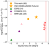 |
Fig. 1. Survey area comparison between previous studies and this work. The filled orange circle represents the estimated survey area of this work, while the star plot denotes the final release status of HSC-VIKING-eRASS. The filled green, purple, and pink triangles denote the survey areas of previous X-ray detected DOG studies in the Chandra Deep Field South (CDFS; Corral et al. 2016), the COSMOS field (Riguccini et al. 2019), and XMM-LSS field (Kayal & Singh 2024), respectively. The red line outlines the extent of the all-sky area. |
The extended ROentgen Survey with an Imaging Telescope Array (eROSITA; Merloni et al. 2020, 2024) is the primary instrument on the Spectrum-Roentgen Gamma (SRG) mission (Predehl et al. 2021; Sunyaev et al. 2021)1. The eROSITA Final Equatorial Depth Survey (eFEDS: Brunner et al. 2022) was released as an X-ray data catalog covering a survey area of ∼140 deg2 (126 < RA [deg] < 146 and −3 < Dec [deg] < 6: hereafter eFEDS footprint; Brunner et al. 2022). The eFEDS footprint reaches a flux limit of f0.5 − 2 keV = 6.5 × 10⁻¹⁵ erg s−1 cm−2, which is 50% deeper than the final integration of the planned four-year program (eRASS8) in the ecliptic equatorial region (f0.5 − 2 keV = 1.1 × 10⁻¹⁴ erg s−1 cm−2; Predehl et al. 2021); therefore, eFEDS is considered to be a representation of the final eROSITA all-sky survey.
The eFEDS main X-ray catalog contains 27 369 point sources (Brunner et al. 2022). In Salvato et al. (2022), a multi-wavelength catalog for these X-ray sources is constructed (hereafter eFEDS multi-wavelength catalog), and the photometric redshift (zphoto) of these X-ray sources is estimated using two different methods: machine learning (Nishizawa et al., in prep.) and SED fitting (Arnouts et al. 1999; Ilbert et al. 2006). For the search of optical and MIR counterparts, DESI Legacy Imaging Surveys Data Release 8 (LS8; Dey et al. 2019) is adopted. LS8 catalog provides not only optical photometry (g, r, and z bands) from the Dark Energy Camera Legacy Survey (DECaLS) but also WISE forced photometry from imaging through NEOWISE-Reactivation (NEOWISE-R; Mainzer et al. 2014) measured in the unWISE maps (Lang 2014; Lang et al. 2016) at the locations of the optical sources. In Liu et al. (2022), the X-ray spectra are fitted by XSPEC (Arnaud 1996) and BXA (Buchner et al. 2014; Buchner 2021), and the X-ray properties (e.g., NH, absorption corrected X-ray intrinsic luminosity between 0.5 keV and 2.0 keV: L0.5 − 2 keV(abs, corr)) are calculated by adopting the spectroscopic redshift (zspec) or the estimated zphot. Given the medium depth and wide survey area of eFEDS, it provides the first X-ray data for the statistical sample of DOGs. The estimated survey area of the DOG survey with eFEDS is 60 deg2, which is 30 times larger area compared to previous X-ray DOGs survey (see Figure 1) and the final survey area of the combined HSC-SSP optical and the final data release of the eROSITA all-sky survey (eRASS) is expected to reach 1000 deg2.
In this paper, the objectives are to select eFEDS-detected DOGs (hereafter eFEDS-DOGs) and report the statistical X-ray properties of eFEDS-DOGs, based on HSC, VIKING, LS8, unWISE, and eFEDS data. The paper is organized as follows: We describe the sample selection of DOGs and the classifications in Section 2. In Section 3, we detail the obtained X-ray properties of DOGs, and we discuss the results in Section 4. Conclusions and a summary are provided in Section 5. Throughout this paper, the adopted cosmology is a flat Universe with H0 = 70 km s−1 Mpc−1, ΩM = 0.3, and ΩΛ = 0.7, which are the same as those adopted in Liu et al. (2022) and Salvato et al. (2022). Unless otherwise noted, all magnitudes refer to the AB system.
2. Data analysis
2.1. Sample selection
In this study, we selected DOGs detected by eROSITA in the eFEDS field (eFEDS-DOGs) by combining HSC-DOGs (Toba et al. 2015; Noboriguchi et al. 2019) with the eFEDS X-ray AGN catalog. The flow chart of our sample selection process is illustrated in Figure 2. We identified a total of 65 eFEDS-DOGs and 74 eFEDS-detected DOGs (the definitions will be described later) within an area of approximately 60 deg2. To construct the multi-wavelength sample, we used the HSC catalog (optical), VIKING catalog (NIR), ALLWISE catalog (MIR), Legacy Survey catalog with unWISE photometry data (MIR), and eFEDS AGN catalog (X-ray).
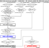 |
Fig. 2. Flow chart of the sample selection for the “eFEDS-detected DOGs” (74 objects) and “eFEDS-DOGs” (65 objects). |
2.1.1. Catalogs
HSC is a wide-field optical imaging camera installed at the prime focus of the Subaru telescope (Furusawa et al. 2018; Kawanomoto et al. 2018; Komiyama et al. 2018; Miyazaki et al. 2018). The S19A catalog, released internally within the HSC survey team, is based on data obtained from March 2014 through April 2019. In the eFEDS footprint region, the status of HSC S19A data covers full colors of grizy and full depth, reaching the limiting magnitudes (5σ, 2″ diameter aperture) with g, r, i, z, and y bands of 26.5, 26.1, 25.9, 25.1, and 24.4 mag, respectively (Aihara et al. 2018b, 2019). In this study, we used a forced photometric catalog of the S19A release (Aihara et al. 2018b), analyzed through an HSC pipeline (hscPipe version 7.9.1; Bosch et al. 2018) developed by the HSC software team using codes from the Large Synoptic Survey Telescope (LSST; LSST Science Collaboration 2009) software (pipline12; Ivezić et al. 2019; Axelrod et al. 2010). Hereafter, we use the cmodel magnitude, estimated by a weighted combination of exponential and de Vaucouleurs fits to the light profile of each object (Lupton et al. 2001; Abazajian et al. 2004), to investigate the photometric properties of the sample after correcting for Galactic extinction (Schlegel et al. 1998).
The VIKING survey is a wide-area NIR imaging survey with five bands (Z, Y, J, H, and Ks bands) observed with the VISTA Infrared Camera on the VISTA telescope (Dalton et al. 2006). We utilized DR4, the final data release catalog supported by the European Southern Observatory2. The limiting magnitudes (5σ, 2″ diameter aperture) for the VIKING Z, Y, J, H, and Ks bands are 23.1, 22.3, 22.1, 21.5, and 21.2 mag, respectively. We used 2″-aperture magnitudes in our analysis, and these magnitudes are also corrected for Galactic extinction (Schlegel et al. 1998).
In this study, we use unWISE data (Schlafly et al. 2019) as MIR data from the LS8 catalog (Dey et al. 2019). WISE observed all-sky in the MIR bands (3.4, 4.6, 12, and 22 μm). The unWISE Catalog, an improvement over the AllWISE catalog (Wright et al. 2010; Cutri et al. 2013; Cutri 2014; Schlafly et al. 2019), provides deeper imaging and better modeling of crowded regions, detecting sources 0.7 magnitudes deeper than those of AllWISE for bands 3.4 μm (W1) and 4.6 μm (W2) (Schlafly et al. 2019). The sensitivities of unWISE catalog at 3.4 (W1), 4.6 (W2), 12 (W3), and 22 (W4) μm bands are generally better than 19.8, 19.5, 16.4, and 14.5 mag, respectively, although sensitivity depends on the sky position (Wright et al. 2010; Cutri et al. 2013; Cutri 2014; Schlafly et al. 2019). We use profile-fitting magnitude from unWISE photometric information measured at the coordinates of LS8 optical sources.
For X-ray data, we utilized the eFEDS AGN catalog (Liu et al. 2022), which contains the best-estimated redshifts by Salvato et al. (2022). Liu et al. (2022) produced the X-ray spectral catalog for 22079 objects with reliable counterparts and with good signal-to-noise. They extracted the X-ray spectra using srctool v1.63 of the eROSITA Science Analysis Software System (eSASS; Brunner et al. 2022). They used multiple models to fit the AGN spectra, and the baseline model was an absorbed power-law with XSPEC terminology of TBabs*zTBabs*powerlaw (Liu et al. 2022). In addition, for bright objects with a soft excess, they added an additional power-law component to the baseline model, creating a “double-power-law” model. On the other hand, for faint objects which are too faint to constrain the spectral shape parameters of the “single-power-law” model, they fixed the X-ray photon index (Γ), the absorbing column density (NH), or both at typical values for the sample (Γ = 2.0 and NH = 0). The Galactic absorption (TBabs) is also applied using the total NH, Gal measured by the neutral HI observations through the HI4PI collaboration (HI4PI Collaboration 2016) in the direction of the eFEDS field. Utilizing the obtained redshift information by Salvato et al. (2022), Liu et al. (2022) derived key AGN properties, including the L0.5 − 2 keV(abs, corr), NH, and Γ.
2.1.2. Clean samples for each catalogs
In selecting DOGs and eFEDS-DOGs, we first established clean samples for HSC, VIKING, LS8, and eFEDS catalogs. For the HSC and VIKING clean sample selection, we refer to the procedures outlined in Toba et al. (2015) and Noboriguchi et al. (2019).
The HSC S19A wide forced catalog initially contains 709 003 990 objects. To ensure proper measurements, we exclude objects with inaccurate photometry as follows (see Figure 2). Firstly, we select 38 537 397 objects in the overlap region between the eFEDS footprint and VIKING survey area (129 < RA [deg] < 141 and −2 < Dec [deg] < 3). Consequently, the survey area in this work is limited to the VIKING region within the eFEDS footprint. We remove objects affected by the edge, saturated pixels, cosmic rays, or bad pixels using flags such as pixelflags_edge, pixelflags_saturatedcenter, pixelflags_crcenter, and pixelflags_bad (Bosch et al. 2018). Objects without a clean centroid measurement in i band are excluded using the flag sdsscentroid_flag. Furthermore, we exclude objects that are not deblended and not unique using the flag isprimary. To eliminate objects with unreliable photometry, we exclude those with a signal-to-noise ratio (SNR) < 5 at i band. In the end, 17 669 962 objects constitute the HSC clean sample.
The VIKING DR4 catalog initially contains 94 819 861 objects. Applying the same region cut as for the HSC clean sample results in 4 792 775 objects. We exclude objects that are not unique or are affected by significant noise using flags such as PRIMARY_SOURCE = 1 and KSPPERRBITS = 0 (Cross et al. 2012). Objects with SNR < 5 at Ks band are also removed. Consequently, 1 354 684 objects form the VIKING clean sample.
The LS8 catalog3 initially contains 1 604 942 717 objects. Applying the region cut as for the HSC clean sample results in 5 085 686 objects. Objects whose flux is affected by other sources are excluded using the flag fracflux_w4 < 0.8. Additionally, objects with SNR < 3 at W4 band are removed. In the end, the LS8 clean sample contains 177 836 objects.
The eFEDS X-ray AGN catalog initially contains 22 079 objects. We exclude objects with a counterpart quality that is not good in multi-wavelength analysis (Salvato et al. 2022) using the flag CTP_quality ≥ 2. Objects with spectroscopic or photometric redshifts, estimated by two different methods (SED fitting and machine learning; Salvato et al. 2022), and with consistent results from both methods are retained using the flag CTP_REDSHIFT_GRADE ≥ 3. Additionally, objects with unreliable NH estimations are excluded using the flag NHclass ≥ 2 (see Liu et al. 2022). In the end, the selection above leaves 17 502 objects form the eFEDS AGN clean sample. However, to investigate X-ray detection rate, we apply the above flags after cross-matched HSC-LS8 DOGs with the eFEDS AGN catalog.
2.1.3. Cross-matching and selection
To minimize misidentification between HSC and unWISE samples (given their typical angular resolutions of ∼0 6 in HSC i band and ∼10″ in WISEW4 band), we employ an optical-NIR color cut since the VIKING survey has spatial resolution of 1.0 arcsec, which is similar one with optical HSC bands (see Toba et al. 2015; Noboriguchi et al. 2019). First, the cross-matched sample between HSC and VIKING contains 1 164 326 objects by nearest neighbor matching within a search radius of 1.0 arcsec. Next, we apply the color cut ((i − Ks)AB ≥ 1.2; Toba et al. 2015; Noboriguchi et al. 2019), and the HSC-VIKING sample comprises 515 030 objects.
For cross-matching the HSC-VIKING sample with the LS8 clean sample with unWISE data, we adopt a search radius of 1.0 arcsec between the coordinates of HSC and LS8 since LS8 coordinates are determined from optical data. This process results in the selection of 17 611 objects (HSC-LS8 sample). To identify DOGs, we apply the DOGs criterion of (i − [22])AB > 7.0 to the HSC-LS8 sample. Consequently, we select 5738 HSC-LS8 DOGs.
We select eFEDS-detected DOGs from HSC-LS8 DOG sample by LS8 ID cross-matching with the sFEDS AGN catalog. A total of 74 eFEDS-detected DOGs are selected. The detected objects with NHclass < 2 are 9 objects, and all of them have CTP_REDSHIFT_GRADE = 3. Hereafter, we treat those objects as eFEDS-detected DOGs with NHclass < 2, but we do not include them for the remaining discussion using L0.5 − 2 keV(abs, corr) and NH.
From the eFEDS-detected DOGs, we further apply additional cut to obtain the sample with reliable X-ray based parameters. We apply the flags (CTP_quality ≥ 2, CTP_REDSHIFT_GRADE ≥ 3, and NHclass ≥ 2) to select 65 objects, hereafter called “eFEDS-DOGs”. This eFEDS-DOGs sample is the primary one for the results using the X-ray properties, while the eFEDS-detected DOGs sample is used for the results not using the X-ray properties. This number difference slightly affects the eFEDS detection rate, which will be discussed in Section 3.2.
Although our sample is based on good redshift quality selection (CTP_REDSHIFT_GRADE ≥ 3), it is worth noting on the available spectroscopic redshift information. Eight objects out of total 65 sources were observed by SDSS spectroscopic follow-up observations (DR18; Almeida et al. 2023) after the construction of the eFEDS AGN catalog, but we did not update that information at this stage and we will discuss their spectroscopic properties in the forthcoming paper. Note that six out of 8 objects have correct spec-z confirmation (|zspec − zphoto|< 0.05) but 2 objects show > 1σ deviation of photo-z uncertainty (|zspec − zphoto|> 1σ). We will not include these two objects in the following results using luminosities and NH since those values could be erroneous ones.
2.1.4. Hard X-ray detected eFEDS-DOGs sample
We also checked whether our HSC-LS8 DOGs have hard X-ray counterparts by utilizing the eFEDS hard band catalog, which is based on the high detection likelihood (DET_LIKE > 10) at the 2.3–5 keV band (Brunner et al. 2022; Nandra et al. 2025). Since the eFEDS hard band catalog contains the information of the optical counterparts including the corresponding optical LS8 coordinates, we performed LS8 ID matching between the HSC-LS8 DOGs and the hard X-ray band catalog. Only one source matches. The source is also one of the 65 eFEDS-DOGs sample (the ID is ID_SRC(main) = 608 or ID_SRC(hard) = 439). As expected from the detection of the both X-ray catalogs, it is a moderately obscured source with log(NH/cm−2) = 21.1, and it is located one of the lowest redshift source at z = 0.60. Since the detection is only one source, we will not discuss the hard X-ray properties of this source, but add one flag “Hard_Detection” and the source is flagged “Y” (see Table A.1 for more details).
2.2. MIR classification of DOGs
We categorized our eFEDS-DOG samples into three types (unclassified DOGs, bump DOGs, and PL DOGs; Noboriguchi et al. 2019) based on the SED, using the classification criterion of Toba et al. (2015). We assumed that the SEDs of eFEDS-DOGs are described by a power-law between NIR and MIR, and we fitted the SED between W2, W3, and W4 bands using a power-law function. With the fitting result, we calculated the expected Ks band flux density described by the extrapolation from the MIR power-law fit ( ). 21 eFEDS-DOGs with fracflux_w2 > 0.8, fracflux_w3 > 0.5, and/or SNR(W2 and/or W3) < 2 were removed from the classification sample, and these objects were classified as unclassified DOGs. We classified the remaining 44 eFEDS-DOGs into bump DOGs and PL DOGs (see Table 1).
Result of the classification of DOGs in the eFEDS footprint.
Bump DOGs are selected using the following criterion:
 (1)
(1)
where fKs is the observed flux density at the Ks band, selecting 3 sources. Subsequently, we classified the remaining 41 eFEDS-DOGs as PL DOGs (i.e.,  ).
).
2.3. Optical classification of DOGs
Following the BluDOGs criterion outlined in Noboriguchi et al. (2019), we conducted a search for BluDOGs within the eFEDS-DOG sample. We estimated the optical spectral slope ( ) by fitting the optical SEDs (HSC g, r, i, z, and y bands). None of our sample fulfilled the BluDOGs classification criterion of
  (Table 1).
However, some SEDs of the eFEDS-DOGs exhibited a flattened SED between the HSC g band and i band, and a power-law SED between optical and MIR bands. Consequently, we identified BluDOG-like eFEDS-DOGs using the MIR classification and the optical spectral slope ( ) obtained by fitting the optical SEDs (HSC g, r, and i bands). Two objects were classified as BluDOG-like, adhering to the criteria of MIR_CLASS = 2 (PL DOGs; see Tables 1 & A.1) and
  .
.
2.4. CIGALE SED fitting
We also calculated the rest-frame AGN 6 μm luminosity (L6 μm), which is used for the discussion on the accretion disk and hot electron corona properties by comparing to L0.5 − 2 keV(abs, corr) (see Section 4.2). Although the rest-frame 6 μm emission is generally dominated by the AGN dust (e.g., Chen et al. 2017), eFEDS-DOGs with high SFR might have non-negligible contribution to 6 μm from the host galaxy component. To remove such contamination, we conducted the SED fitting of eFEDS-DOGs by using the Code Investigating GAlaxy Emission (CIGALE; Burgarella et al. 2005; Noll et al. 2009; Boquien et al. 2019). In this study, we utilized the most up-to-date veresion called the CIGALE 2022.1 (Yang et al. 2022). Since the SEDs of eFEDS-DOGs cover the wavelength range from optical i band to WISE W4 (22 μm), we followed the same model with Noboriguchi et al. (2022), which characterized the SED with the combination of three main components: a direct stellar component, a host galaxy dust emission (hereafter star formation component), and an AGN component (direct AGN emissions and AGN heated dust emissions). The details of the parameter setting are summarized in Appendix B and in Table B.1.
Figure 3 shows the examples of the SED fitting, and the modeled spectra nicely reproduce the observed SEDs in the range of interests, especiallly around rest-frame 6 μm. We then estimated the L6 μm from the decomposed AGN dust component. Overall, the estimated L6 μm have slightly smaller values with 0.28 dex on average (see Figure 4), compared to the rest-frame 6 μm luminosity interpolated from the nearby WISE W1, W2, and W3 bands.
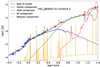 |
Fig. 3. Example of the SED fitting result. The blue, green, and red plots represent the HSC, VIKING, and WISE photometric data, respectively. The black, blue, green, red, and orange lines correspond to the best-fit model, stellar component, AGN component, star formation (SF) component, and nebular component, respectively. |
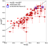 |
Fig. 4. L6 μm estimated by CIGALE ( |


3. Results
3.1. Basic sample properties of eFEDS-DOGs
3.1.1. Distribution in the magnitude planes of MIR and optical bands
Figure 5 shows the distribution of 74 eFEDS-detected DOGs on the WISEW4 (22 μm) band and HSC iAB band diagram. Red, orange, and blue stars represent eFEDS-DOGs, eFEDS-detected DOGs with NHclass < 2, and BluDOG-like eFEDS-DOGs, respectively. The other X-ray detected DOGs in previous studies are also overlaid in the same plane, and their total number is 106 sources (Lanzuisi et al. 2009; Corral et al. 2016; Riguccini et al. 2019; Toba et al. 2020; Zou et al. 2020; Kayal & Singh 2024).
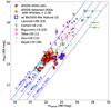 |
Fig. 5. MIR band versus optical band magnitudes of eFEDS-DOGs as well as previous X-ray detected DOGs. Red and orange stars denote eFEDS-DOGs and eFEDS-detected DOGs with NHclass < 2, respectively. Blue squares show eFEDS-DOGs with the BluDOG-like feature. Lime, Green, purple, magenta, cyan, and pink plots denote X-ray detected DOGs from Lanzuisi et al. (2009), Corral et al. (2016), Riguccini et al. (2019), Toba et al. (2020), Zou et al. (2020), and Kayal & Singh (2024), respectively. For the sample fainter than mMIR > 15 mag (e.g., Lanzuisi et al. 2009; Corral et al. 2016; Riguccini et al. 2019), we utilized Spitzer/MIPS 24 μm bands as mMIR. The optical bands were obtained from the Hubble/ACS F775 band (Corral et al. 2016), Suprime-Cam iAB′ bands (Riguccini et al. 2019) and heterogeneous optical magnitudes by Vizier with the nearest matching with < 3 arcsec (Lanzuisi et al. 2009). The solid red line represents the DOGs criterion, and three dashed red lines denote (i − W4)AB = 8.0, 9.0, and 10.0. The numbers in parentheses indicate the number of objects. |
Figure 5 shows that the number of X-ray-detected DOGs has almost doubled from 106 to 180, and eFEDS-detected DOGs occupy the unique parameter range with (iAB, mMIR, AB) = (22–24, 14–16) mag, which were not explored in the previous X-ray surveys. This is thanks to the wide-area coverage of the combination of eFEDS and WISE, resulting in the detections of relatively brighter (originating from the WISE W4 limiting magnitude of mW4 < 15.5 mag) and relatively rarer DOG populations that were missed in the previous X-ray survey with < 10 deg2 (Lanzuisi et al. 2009; Corral et al. 2016; Riguccini et al. 2019; Toba et al. 2020). On the other hand, Zou et al. (2020) covers the brightest end among the X-ray detected DOGs with iAB < 22 mag. This is because their sample selection originates from the combination of the SDSS-WISE DOGs and heterogeneous but very wide-area XMM-Newton Slew survey area, whose limiting magnitude of iAB ≲ 22 mag (Toba & Nagao 2016).
Additionally, our sample contains wide range of (i − [22])AB colors, covering nine eFEDS-DOGs with extremely red color of (i − [22])AB ≥ 9.0 mag. Corral et al. (2016), Riguccini et al. (2019), and Kayal & Singh (2024) also exhibit very red color objects similar to our sample, and we discuss those populations in Section 4.1.
3.1.2. L–z plane
Figure 6 shows the rest-frame 6 μm AGN luminosity (L6 μm) as a function of redshift. Our eFEDS-DOGs cover wide redshift range of 0.5 ≲ z < 2.5 with average of  (see Table 2) and wide luminosity range of
  with average of
  (Table 2). Figure 6 also shows the comparison from the sample made by Spitzer Wide-area InfraRed Extragalactic (SWIRE: Lonsdale et al. 2003) survey (Lanzuisi et al. 2009), SDSS-WISE survey (Toba et al. 2020; Zou et al. 2020), HSC-MIPS survey (Kayal & Singh 2024), and hot DOG surveys (Stern et al. 2014; Assef et al. 2016; Ricci et al. 2017a; Vietri et al. 2018; Zappacosta et al. 2018). Our sample covers higher-z sources thanks to relatively deeper X-ray follow-ups, as well as the power of deep photometries of Subaru/HSC.
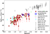 |
Fig. 6. Rest-frame 6 μm AGN luminosity (L6 μm) as a function of redshift. The L6 μm is estimated from the decomposed AGN dust component as a result of the SED fitting, as discussed in Section 2.4. The red stars denote the eFEDS-DOGs, and the blue squares denote eFEDS-DOGs with the BluDOG-like feature. The lime, magenta, cyan, and pink plots represent X-ray detected DOGs from Lanzuisi et al. (2009), Toba et al. (2020), Zou et al. (2020), and Kayal & Singh (2024), respectively. As for the hot DOG samples, black triangle, downward triangle, pentagon, square, and cross represent data from Stern et al. (2014), Assef et al. (2016), Zappacosta et al. (2018), Ricci et al. (2017a) and Vito et al. (2018), respectively. |
Summary of physical parameters
Figure 7 shows the absorption corrected 0.5-2 keV luminosity (L0.5 − 2 keV(abs, corr)) as a function of redshift. For the comparison samples (Lanzuisi et al. 2009; Corral et al. 2016; Riguccini et al. 2019; Toba et al. 2020; Zou et al. 2020; Kayal & Singh 2024), L0.5 − 2 keV(abs, corr) values were extrapolated from their L2 − 10 keV(abs, corr) values by assuming a photon index of Γ = 1.8 (e.g., Ricci et al. 2017a). This clearly shows that eFEDS-DOGs cover a relatively luminous end at each redshift. Particularly, the eFEDS-DOGs with z > 1 consist of the most luminous X-ray sample among the X-ray detected DOGs, reaching L0.5 − 2 keV(abs, corr) > 1045 erg s−1. Moreover, the redshift distribution of eFEDS-DOGs covers a wide redshift range from z = 0.5 to z = 2.5, bridging the gap between the low-z samples of z < 1 (Toba et al. 2020; Zou et al. 2020) and higher-z samples (Lanzuisi et al. 2009; Corral et al. 2016; Riguccini et al. 2019, 1 < z < 4).
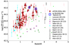 |
Fig. 7. L0.5 − 2 keV(abs, corr) as a function of redshift. The plots are same as in Figure 5. One object presented in Corral et al. (2016) is not shown in this figure due to its low luminosity (log(L0.5 − 2 keV(abs, corr)/erg s−1) < 42.0). |
Figure 7 also shows that BluDOG-like eFEDS-DOGs exhibit redshifts between 1.5 and 2.3. This is a natural outcome since the redshifted C IVλ1549 emission line joins the HSC g bands (Noboriguchi et al. 2022, 2023), which makes the optical color bluer within the redshift range of 1.6 < z < 2.5.
3.2. Basic properties of eFEDS-undetected DOGs
Non-detection by eROSITA also gives important information either on the gas obscuration and/or the accretion disk properties of the AGN in the DOGs. The majority of DOGs in the eFEDS footprint are not detected by eROSITA, resulting in a low detection rate of 1.3% (74 sources out of 5738). Given the energy band of eROSITA at E = 0.5–2.0 keV, detection by eROSITA implies that their column densities are NH < 1023 cm−2 (Gilli et al. 2007). On the other hand, non-detection provides a lower limit on NH, and most undetected DOGs are expected to have NH > 1023 cm−2, especially at z > 0.5.
To estimate the lower bound of NH for eFEDS-undetected DOGs, we utilized the luminosity relation between L2 − 10 keV(abs, corr) and L6 μm (e.g., Chen et al. 2017), and extrapolated L0.5 − 2 keV(abs, corr) by assuming a photon index of Γ = 1.8. Non-detection by eROSITA also provides an upper limit on the absorption-uncorrected 0.5–2 keV luminosity. We estimated the required lower bound of NH to fulfill the gap between the two values. In this estimation, we calculated NH only for eFEDS-undetected PL DOGs (291 objects; see Table 1), since PL DOGs exhibit clear AGN features, while bump DOGs do not necessarily host a central AGN.
Figure 8 displays the distributions of eFEDS-undetected PL DOGs in terms of estimated L0.5 − 2 keV(abs, corr) as a function of redshift. These L6 μm values are simply estimated from the MIR best-fit power-law between the W2 and W4 bands (see Section 2.2). However, objects undetected by W2 and/or W3 bands do not have a best-fit power-law function. Therefore, we estimated L6 μm with/without an upper limit flag, as shown in Appendix C and Table C.1. The majority of eFEDS-undetected PL DOGs are positioned above the line of NH > 1023 cm−2, especially at z > 0.5. This boundary line is consistent with the expected upper-bound of NH for eROSITA detectable sources.
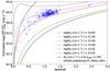 |
Fig. 8. Distribution of the eFEDS-undetected PL DOGs in the plane of L0.5 − 2 keV(abs, corr) and redshift. The L0.5 − 2 keV(abs, corr) were estimated from the obtained L6 μm, by utilizing the luminosity relation between L2 − 10 keV(abs, corr)–L6 μm (e.g., Chen et al. 2017), and extrapolated the expected L0.5 − 2 keV(abs, corr) by assuming the photon index of Γ = 1.8. The blue crosses represent the eFEDS-undetected PL DOGs. The solid blue, orange, green, red, purple, and brown lines represent the limiting luminosities between 0.5 and 2.0 keV with corresponding log(NH/cm−2) of f20, 21, 22, 23, 23.25, and 23.5, respectively. For calculating the limiting luminosities, we utilize a flux limit of f0.5 − 2 keV = 6.5 × 10⁻¹⁵ erg s−1 cm−2. The solid black line represents the upper bound of the expected X-ray luminosities by assuming that the eFEDS X-ray band is dominated by the X-ray scattered component with fscatt = 1.4%. This is equivalent to a value that is 100/1.4 times above the curve of NH/cm−2 = 0. |
One might question whether the non-detection of X-ray “scattered” emission can provide meaningful constraints on our non-detection. The scattered X-ray emission contributes in the soft X-ray bands, especially when the targets are the obscured AGN, since the scattered emission originates from the gas-free polar area of the obscuring torus. Assuming an average scattered emission fraction of fscatt = 1.4% (Ricci et al. 2017a), the X-ray non-detection places an upper limit on the expected X-ray luminosity that is approximately a factor of 70 above the curve for NH/cm−2 = 0. As shown in Figure 8, all the estimated L0.5 − 2 keV(abs, corr) values lie below the expected upper-limit curve, consistent with this picture.
Figure 9 shows the NH distributions of eFEDS-DOGs, eFEDS-undetected DOGs, and comparison samples. This demonstrates that the majority of DOGs host heavily obscured AGNs with NH > 1023 cm−2, assuming that all DOGs follow the L2 − 10 keV(abs, corr)–L6 μm relation (e.g., Chen et al. 2017). In contrast, eFEDS-DOGs represent a rare population among DOGs, with smaller NH values (NH < 1023 cm−2). Figure 9 also demonstrates that eFEDS-DOGs in this study expand the NH range for X-ray detected DOGs and eFEDS-DOGs contain even unobscured AGNs (gas+dust unobscured DOGs) with NH < 1022 cm−2, while previous X-ray detected DOGs exhibit NH > 1022 cm−2, representing only obscured AGNs (Lanzuisi et al. 2009; Corral et al. 2016; Riguccini et al. 2019; Toba et al. 2020; Zou et al. 2020). Among the sample from Kayal & Singh (2024), five objects have 21.5 < log(NH/cm−2) < 22.0, while the majority show log(NH/cm−2) > 22.0. In contrast, the presence of objects with log(NH/cm−2) < 21.5 in our sample represents a truly unique population.
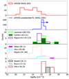 |
Fig. 9. NH histogram with a bin width of 0.5 dex. Top panel: A red histogram represents eFEDS-DOGs. Second panel: A blue histogram represents eFEDS-undetected PL DOGs, indicating lower limits on log(NH/cm−2). Note that only this panel uses a different binning scheme: 22.0–23.0, 23.00–23.25, and 23.25–23.50. Third panel: Lime, green and purple histograms represent Lanzuisi et al. (2009), Corral et al. (2016) and Riguccini et al. (2019), respectively. Fourth panel: Magenta, cyan, and pink histograms represent Toba et al. (2020), Zou et al. (2020), and Kayal & Singh (2024), respectively. Bottom panel: black, gray, and brown histograms represent Assef et al. (2016), Ricci et al. (2017a), and Zappacosta et al. (2018), respectively. |
Another important possibility for the origin of the X-ray non-detection in eFEDS is that the DOGs are intrinsically X-ray weak. Our results are based on the assumption that AGNs in DOGs would follow the L2 − 10 keV(abs, corr)–L6 μm relation, but some AGN populations lie well below this relation curve. Yamada et al. (2021, 2023) demonstrated that local Ultra-Luminous Infrared Galaxies (ULIRGs) at z < 1 exhibit extremely X-ray weak features that do not follow the standard L2 − 10 keV(abs, corr)–L6 μm relation. Similarly, extremely dust-obscured AGNs, known as hot DOGs, also exhibit a similar trend at 1 < z < 3 (Eisenhardt et al. 2012; Ricci et al. 2017a; Vito et al. 2018; Díaz-Santos et al. 2021). Given that all these populations (ULIRGs, hot DOGs, and DOGs) are known to display major merger features (Veilleux et al. 2002; Ishida 2004; Kartaltepe et al. 2010 for ULIRGs and Melbourne et al. 2009; Bussmann et al. 2009b, 2011 for DOGs), our eFEDS non-detected DOGs at 0.5 < z < 1.5 might also belong to such intrinsically X-ray weak sources.
If eFEDS-undetected DOGs follow a similar trend to local ULIRGs or hot DOGs at 1 < z < 3, the expected L0.5 − 2 keV(abs, corr) would decrease by a factor of up to 3 (see Ricci et al. 2017a; Yamada et al. 2023), and thus their expected lower limits of NH would also decrease to NH > 1022 cm−2. A deeper hard X-ray observation at E > 2 keV is crucial to disentangle the degeneracy between obscuration (high NH) and the intrinsic X-ray weak scenario.
In summary, the eROSITA non-detection provides crucial information suggesting that most eFEDS non-detected DOGs either host heavily obscured AGNs with NH > 1023 cm−2 (see also Toba et al. 2022; Fukuchi et al. 2025), exhibit extremely weak X-ray features, or both. On the other hand, a large fraction (> 50%) of eFEDS-DOGs show unobscured AGN properties. eROSITA opens up a new population of DOGs, the gas+dust unobscured DOGs, which might be in a transitional phase from heavily obscured to decreased gas-covering fraction. This population could be a key tracer of the final phase of major merger scenarios (e.g., Hopkins et al. 2008) and/or gas-obscured SMBH growth (Ricci et al. 2022, 2023).
4. Discussions
4.1. Variations in gas-to-dust ratios
The finding of gas+dust unobscured DOGs with NH < 1022 cm−2, as shown in Figure 9, provides several key insights on the gas and dust properties and their geometries for eFEDS-DOGs. Figure 10 illustrates the distribution of X-ray detected DOGs in the plane of NH (gas absorption) and (i − W4)AB (dust extinction). While previous X-ray detected DOGs are clustered exclusively in the obscured AGN region with NH > 1022 cm−2, the eFEDS-DOGs represent relatively gas+dust unobscured AGNs but exhibit an extremely red (i − W4)AB color with 7 [mag] < (i − W4)AB < 10 [mag].
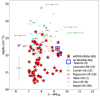 |
Fig. 10. (i − W4)AB vs. NH. See Figure 5 for the description of each plots. A gray plot with error bars represents typical standard deviations of (i − W4)AB and NH, and the standard deviations of (i − W4)AB and NH are 0.21 mag and 0.69 dex, respectively. |
These eFEDS-DOG sources do not demonstrate a clear relationship between (i − W4)AB and NH. One possibility is that the physical locations of media responsible for dust and gas absorption for eFEDS-DOGs might be different. Such possibilities were reported in several observational studies for AGN obscurations, suggesting the presence of dust-free gas that is responsible for part of the X-ray absorption (e.g., long-term X-ray variabilities; Maiolino et al. 2010; Risaliti et al. 2007, 2011; Markowitz et al. 2014), (the expected location of Fe Kα line emitting material; Minezaki & Matsushita 2015; Gandhi et al. 2015), (e.g., the discrepancy between the gas covering fraction and the dust one; Davies et al. 2015; Ichikawa et al. 2019a).
On the other hand, our result shows an opposite trend; a lack of gas obscuration into the line-of-sight, but the existence of dust absorption (extinction) on a larger physical scale. Figure 11 illustrates one possible schematic sketch to explain the obtained (i − W4)AB vs. NH relationship for eFEDS-DOGs. In the left upper panel (A in Figure 11 and Table 3), heavy obscuration is caused by both gas and dust. These objects exhibit log(NH/cm−2) > 23 and higher (i − W4)AB values, suggesting that both the UV emitting region in the accretion disk and the X-ray emission region are heavily obscured by gas and dust. The majority of eFEDS-undetected DOGs, with an estimated lower limit of log(NH/cm−2) > 23, likely exhibit a similar gas and dust geometry as depicted in (A) of Figure 11.
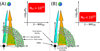 |
Fig. 11. Illustration explaining the (i − W4)AB vs. NH relationship based on geometry. Filled black, gray, and cyan circles denote SMBHs, dust clumps, and gas absorbers, respectively. Filled pink ellipses and white trapezoids represent X-ray sources and accretion disks, respectively. Cyan and orange arrows indicate fluxes from X-ray sources and accretion disks, respectively. |
On the other hand, the right upper panel (B in Figure 11 and Table 3), heavy obscuration is caused by dust, but the gas absorber does not cover the line-of-sight. Considering the X-ray emitting size is extremely compact with < 10 Rg (e.g., Dai et al. 2010; Morgan et al. 2010) while optical and UV-emitting region of accretion disk is much larger, with R ≈ 100–103Rg (Kato et al. 2008; Morgan et al. 2010; Ichikawa et al. 2019b), these objects show unobscured properties with log(NH/cm−2) < 22 because of the lack of obscuring gas, but it still maintains high (i − W4)AB values due to the significant dust extinction and dust re-emission. This dust and gas geometry suggests a transition phase between an obscured AGN and an optically selected quasar in the gas-rich major merger scenario (Hopkins et al. 2008). The majority of eFEDS-DOGs, with log(NH/cm−2) < 22 and (i − W4)AB > 7 [mag], likely exhibit the geometry of gas and dust similar to (B) in Figure 11.
The difference between eFEDS-DOGs and eFEDS-undetected DOGs: physical parameters, geometry, and population.
4.2. X-ray and 6 μm luminosity correlation
Our sample contains both of MIR and X-ray luminosity information of a statistically significant number of eFEDS-DOGs, and their locations in the luminosity-luminosity plane between MIR and X-ray enable us to discuss a rough indication of the Eddington ratio of the eFEDS-DOGs. The tight correlation between X-ray and MIR luminosities for AGNs has been reported in numerous studies. The trend shows that almost 1:1 relation up to  (e.g., Gandhi et al. 2009; Asmus et al. 2015; Ichikawa et al. 2012, 2017, 2019a; Matsuta et al. 2012; Mateos et al. 2015; Yamada et al. 2023), above which X-ray luminosities show a saturation and thus the flatter trend (e.g., Stern 2015; Chen et al. 2017; Toba et al. 2019, 2022; Ichikawa et al. 2023). On the other hand, extremely IR luminous DOGs, hereafter hot-DOGs (e.g., Eisenhardt et al. 2012; Díaz-Santos et al. 2021), are known to have more X-ray deficit feature compared to the MIR and X-ray relation discussed above, suggesting that hot-DOGs have higher Eddington ratio, possibly exceeding the super-Eddington limit (Stern et al. 2014; Assef et al. 2016; Ricci et al. 2017a; Zappacosta et al. 2018; Vito et al. 2018).
Figure 12 shows a luminosity correlation between the rest-frame 6 μm (L6 μm) and L0.5 − 2 keV(abs, corr) of our eFEDS-DOGs sample. The expected curve of Eddington ratio of λEdd = 0.1, 0.3, and 1.0 are also over-plotted (Toba et al. 2019). Our eFEDS-DOGs nicely cover the L6μm luminosity gap between high-z (z > 2) IR luminous hot DOGs at  and local U/LIRGs at
  (Yamada et al. 2023). Overall, most eFEDS-DOGs follow the luminosity relation of Chen et al. (2017) (hereafter referred to as the Chen relation). This suggests that, on average, eFEDS-DOGs do not exhibit extremely high Eddington ratios as seen in hot DOGs, but rather have Eddington ratios similar to quasars (
 ) in comparable MIR luminosity ranges (e.g., Kollmeier et al. 2006). Similarly, the sources from Kayal & Singh (2024) exhibit a comparable distribution in Figure 12, overlapping well with our eFEDS-DOGs sample. This further supports the idea that DOGs in general tend to populate this parameter space, as also indicated by the findings of Kayal & Singh (2024). However, focusing on individual sources, the scatter of eFEDS-DOGs in Figure 12 is large, with an λEdd standard deviation of σ = 0.45 dex; some eFEDS-DOGs deviate by more than 0.5 dex above or below the Chen relation. Since we use a simple X-ray spectral fitting with an average uncertainty in log(NH/cm−2) of 0.69 dex (Section 2.1.1), this may partially contribute to the observed scatter. Beyond this methodological uncertainty, we discuss possible physical origins of the scatter.
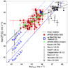 |
Fig. 12. Luminosity correlation between the luminosities at absorption corrected 0.5–2 keV (L0.5 − 2 keV(abs, corr)) and 6 μm (L6 μm). The symbols are the same as in Figure 5. The open green circles show the mean and standard deviation of L0.5 − 2 keV(abs, corr) for the eFEDS-DOG sample, and each bin has a range of log L0.5 − 2 keV(abs, corr) = 43.8–44.8, 44.8–45.3, 45.3–45.8, and 45.8–46.3. Open triangle, inverted triangle, square, pentagon, and crosses represent IR luminous quasars or hot-DOGs (Eisenhardt et al. 2012; Díaz-Santos et al. 2021) from Stern et al. (2014), Assef et al. (2016), Ricci et al. (2017a), Zappacosta et al. (2018), and Vito et al. (2018), respectively. Open hexagon represents a sample of Yamada et al. (2023); local (z < 0.1) U/LIRGs with a final merger stage, with two nuclei in common envelope (stage = “D”). The solid black line represents the slope in the study of optically selected quasars at 1.5 < z < 3, named Chen relation in this study (Stern 2015; Chen et al. 2017). The solid, dashed, and dotted blue lines represent the expected location of Eddington ratio of λEdd = 1.0, 0.3, and 0.1, respectively, estimated by Toba et al. (2019). Note that original Chen relation and λEdd lines are defined between L2 − 10 keV(abs, corr) and L6 μm. We convert the original one to the L0.5 − 2 keV(abs, corr)–L6 μm relation by assuming Γ = 1.8. |
One possible origin of this deviation is the difference in Eddington ratio for eFEDS-DOGs, particularly those below the Chen relation. The eFEDS-DOGs at ∼1 dex below the Chen relation align closely with the λEdd = 1 line around L6 μm ∼ 1045.5 erg s−1, suggesting that they are in the Eddington-limit phase (or possibly in a super-Eddington phase). Objects with high Eddington ratios may be undergoing more rapid mass accretion (known as the Slim disk model; Abramowicz et al. 1988). In this model, when the mass accretion rate significantly exceeds the Eddington rate, radiation becomes trapped within the accreting matter before escaping by radiative diffusion, resulting in a radiatively inefficient state (e.g., Ohsuga et al. 2009, 2005; McKinney et al. 2014; Inayoshi et al. 2016, 2020; Takeo et al. 2020). According to this model, the inner region (X-ray emission region) of the accretion disk is expected to be thicker than the outer accretion disk (e.g., Ohsuga et al. 2009). Consequently, photons from the accretion disk may not reach the inner region due to the X-ray-emitting region being covered by a thick disk, resulting in X-ray weakness, as the reduced photon supply into the X-ray-emitting region diminishes their observed luminosity. A similar trend was also reported in several hot DOGs and X-ray weak AGNs with super-Eddington signature (see Figure 12), showing extremely X-ray weak features (e.g., Stern et al. 2014; Assef et al. 2016; Ricci et al. 2017a; Vito et al. 2018; Zappacosta et al. 2018; Yamada et al. 2023) as well as recently reported “little red dots” discovered by JWST with more extreme X-ray “deficit” features (Kocevski et al. 2024; Yue et al. 2024). The eFEDS-DOGs at ∼1 dex below the Chen relation might be low-z (z ∼ 1) and low L6 μm analogous sources of such hot DOG samples found mostly at z > 2.
Figure 12 also shows sources above the Chen relation, up to +0.5 dex. The origins of such a deviation have three possibilities: (1) over-estimation of photo-z, (2) objects with a jet, (3) lensed objects. The first possibility is that the photo-z values of those sources might be over-estimated. The over-estimation of photo-z causes the boost of both luminosities by holding the 1:1 relation. In this case, such sources deviate from the Chen relation that has the shallower slope in the high luminosity end. Two eFEDS-DOGs located more than +0.5 dex above the Chen relation exhibit L0.5 − 2 keV(abs, corr) ∼ 1045 erg s−1 (see Figure 12), with objects located around z ∼ 1.5 (see Figure 7). Assuming that the corrected redshifts have the median value of eFEDS-DOGs sample of z ∼ 1, the boost factor μ of both luminosities from z ∼ 1 to 1.5 is μ ≈ 3, mitigating the gap for most of the sources. However, since we selected the eFEDS clean sample with CTP_REDSHIFT_GRADE ≥ 3 (see Section 2.1.2), the likelihood of overestimating the photo-z of eFEDS-DOGs appears to be low.
The second possibility is that those sources have prominent jet emission, or radio-loud eFEDS-DOGs. The jet emission of those sources can contaminate the X-ray bands, boosting the observed X-ray emission (e.g., Blazars and some radio-loud AGNs; Miller et al. 2011; Wu et al. 2013; Ghisellini et al. 2017; Zhu et al. 2020). In Matsuta et al. (2012), blazars and radio-loud AGNs exhibit a 1:1 relation between LX and LMIR, suggesting that the sub-sample of eFEDS-DOGs at +0.5 dex from the Chen relation may have radio jets, which should be luminous in the radio wavelength. However, this scenario would be unlikely, since only one source at least 0.5 dex above the Chen relation is detected in the VLA/FIRST 1.5 GHz (Becker et al. 1995; White et al. 1997; Helfand et al. 2015) or VLASS 3 GHz radio bands (Lacy et al. 2020). In addition, the median X-ray photon index of these sources is Γ = 1.95. Thus they do not show the characteristic feature of radio-jet in X-ray spectra, which tend to show a shallower photon index, characterized by  (e.g., Ighina et al. 2019).
The final possibility is the scenario that the emission of those sources is gravitationally lensed, boosting the both MIR and X-ray luminosities a 1:1 relation (e.g., Connor et al. 2021; Chan et al. 2024). Assuming a tenfold increase in luminosity for the sub-sample of eFEDS-DOGs at +0.5 dex, they align with the Chen relation. The magnification factor can reach η = 10–500 (Glikman et al. 2018; Fan et al. 2019; Fujimoto et al. 2020), thus the de-lensed luminosities of those sources can join the 1:1 relation in the luminosity-luminosity plane.
In summary, at present, we cannot conclude which of the three scenarios is preferable. Additional follow-up observations, such as optical spectroscopy to determine spectroscopic redshifts (for scenario 1), deeper radio observations (for scenario 2), and/or high spatial resolution imaging (for scenario 3), are necessary to distinguish between these three scenarios.
4.3. Eddington ratio and other properties of eFEDS-DOGs
The location of sources in Figure 12 allows us to estimate λEdd, which enables us to compare λEdd with other parameters obtained by X-ray observations. Several observational X-ray spectral studies of AGNs and quasars indicate that photon index Γ changes as a function of λEdd (see Boller et al. 1996; Shemmer et al. 2008; Risaliti et al. 2009; Brightman et al. 2013; Trakhtenbrot et al. 2017), which is thought to originate from the change of the coronal properties around the accretion disk, specifically a plasma parameter (kTe) and a plasma optical depth (τ), where k and Te are the Boltzmann constant and electron temperature, respectively (Titarchuk & Lyubarskij 1995; Zdziarski et al. 1996; Ishibashi & Courvoisier 2010).
Figure 13 shows the Γ–λEdd relation of eFEDS-DOGs, with Γ and λEdd of eFEDS-DOGs being Γ = 1.95 ± 0.15 and log λEdd = −0.64 ± 0.27, respectively. Although the median value of eFEDS-DOGs is slightly below the Γ–λEdd relation obtained by Brightman et al. (2013), it still falls within the uncertainty range, considering the large uncertainties in our λEdd estimates. This trend is also seen when comparing eFEDS-DOGs with other X-ray detected quasars in the plane of Γ as a function of redshift, as shown in Figure 14. Our averaged values are largely consistent with previous studies at z ∼ 1–2, suggesting that the coronal properties of eFEDS-DOGs are similar to optically selected quasars at similar redshifts.
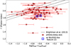 |
Fig. 13. Γ–λEdd diagram. The symbols are the same as in Figure 5. Solid and dashed black lines represent the Γ–λEdd relation and ±1σ lines from Γ–λEdd relation (Brightman et al. 2013). |
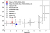 |
Fig. 14. Γ–z diagram. The symbols are the same as in Figure 5. Open diamond, inverted triangle, hexagon, square, triangle, circle, and pentagon plots denote X-ray detected quasars from Vignali et al. (2005), Piconcelli et al. (2005), Shemmer et al. (2006), Just et al. (2007), Nanni et al. (2017), Vito et al. (2019), and Wang et al. (2021), respectively. |
Figure 15 shows λEdd of eFEDS-DOGs as a function of redshift. The underlying gray contour shows the number density of SDSS quasars in the plane (Shen et al. 2011). Note that the log λEdd values for the X-ray detected DOGs from Kayal & Singh (2024) are not directly taken from their study but are instead estimated using the method of Toba et al. (2019) based on L6 μm and L0.5 − 2 keV(abs, corr). This approach was adopted to maintain consistency with our analysis. The log λEdd values of SDSS quasars, eFEDS-DOGs, and BluDOG-like eFEDS-DOGs at each redshift are summarized in Table 4. At each redshift range, the average λEdd of eFEDS-DOGs is higher than those of SDSS quasars, but they are again within the mutual scatter. This result supports that our eFEDS-DOGs sample has similar level or possibly more rapidly growing SMBHs compared to SDSS quasars at each redshift, but roughly half of them are obscured by gas with log(NH/cm−2) > 22 .
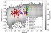 |
Fig. 15. log λEdd as a function of redshift. The gray 2D histogram represents the number density of SDSS quasars (Shen et al. 2011). Red stars and blue squares denote eFEDS-DOGs and BluDOG-like eFEDS-DOGs, respectively. Orange, green, purple, cyan, pink, and lime green hexagons denote BluDOGs (Noboriguchi et al. 2022), extremely red quasars (ERQs: Perrotta et al. 2019), hot DOGs (Wu et al. 2018), DOGs (Melbourne et al. 2011), X-ray detected DOGs (Kayal & Singh 2024), and CT DOG (Toba et al. 2020), respectively. |
log λEdd distribution at each redshift range.
The results presented above indicate that the eFEDS-DOGs exhibit similar X-ray coronal and accretion disk properties to optically bright quasars within a similar redshift range. However, the central engine of eFEDS DOGs remains obscured by dust and gas. This dust and gas-rich environment surrounding the central engine positions eFEDS DOGs uniquely in the plane of NH vs λEdd, as shown in Figure 16. The solid black line represents the effective Eddington limit (see also Fabian et al. 2006, 2009; Ricci et al. 2017b) derived from equation (6) in Ishibashi et al. (2018), assuming IR and UV opacities (κIR and κUV) of κIR = 0 and κUV = 200 cm2 g−1.
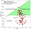 |
Fig. 16. NH–λEdd diagram. The symbols are the same as in Figure 5. A gray plot with error bars denotes typical standard deviations of NH and λEdd. The standard deviations of NH and λEdd are 0.69 dex and 0.18 dex, respectively. Dashed and solid black lines denote log(NH [cm−2]) = 22.0 and equation (6) in Ishibashi et al. (2018). Filled green region shows a forbidden region. |
In this plane, long-live clouds can survive against radiation pressure (“long-lived obscuration” in Figure 16), while absorbed objects at low column densities may appear above their effective Eddington limit due to the presence of dust lanes in the galaxy (“dust lanes” in Figure 16). AGNs in the “forbidden region” are expected to have short-lived obscuration due to significant radiation pressure on the absorbing clouds. Therefore, AGNs do not stay in this region for prolonged periods, suggesting that they are in a “blowout” phase. Out of 63 eFEDS-DOGs, 25 sources (including two bluDOG-like eFEDS-DOGs) are in the forbidden region. Given that 23 objects from the Kayal & Singh (2024) DOG sample are also found in the forbidden region, the presence of nearly half of the eFEDS-DOGs in this region further supports the expectation that X-ray detected DOGs tend to be in blow-out phase. This result supports the idea that eFEDS-DOGs in the forbidden region experience the gas outflow of the obscuring material, which would eventually lead to a decrease in NH. Consequently, the sources would be preferentially observed as unobscured AGNs (Ricci et al. 2022, 2023). Our results indicate that unobscured eFEDS DOGs would be such sources. Thus, eFEDS-DOGs are prominent candidates in a previously overlooked transitional phase between obscured AGNs and optically selected quasars (see also Section 4.1).
4.4. Lifetime of eFEDS-DOGs
eROSITA revealed newly X-ray-detected DOGs, which constitute only 1.3% (74/5738) of the total population; however, this small fraction may represent a transient phase from highly obscured AGNs to unobscured ones. This rarity would give us important information on the lifetime of such a transient phase.
The lifetime of HSC-WISE DOGs at z ∼ 1 is expected to be approximately 40 Myr, as suggested by the DOG duty cycle (Toba et al. 2017). Assuming that eFEDS-DOGs represent one stage in the gas-rich major merger scenario, the lifetime of eFEDS-DOGs can be roughly estimated to be ∼0.5 Myr, given their abundance of 1.3% (74/5738) among all DOGs. This number fraction is similar to that of BluDOGs in DOGs (Noboriguchi et al. 2019). We note that eFEDS-undetected DOGs may include objects such as eFEDS-DOGs viewed from an edge-on angle. Therefore, the estimated 0.5 Myr should be treated as a lower limit for the early transition phase between an obscured AGN and an unobscured quasar (see Section 4.1).
4.5. BluDOG-like eFEDS-DOGs
Blue-excess objects in dusty AGNs are considered to represent a dusty outflow phase (Noboriguchi et al. 2019), and BluDOG spectra exhibit a blue tail on the C IV emission line (Noboriguchi et al. 2022), suggesting that the blue tail is evidence of nucleus outflow. Additionally, some BluDOGs show broad emission lines that enable us to estimate the black hole mass and thus the Eddington ratio (Noboriguchi et al. 2022). Their Eddington ratio shows λEdd ≳ 1, suggesting that they are undergoing super-Eddington accretion. Recently, Noboriguchi et al. (2023) identified high-z BluDOG candidates from JWST-ERO high-z galaxy samples at 5 < z < 7 (e.g., Akins et al. 2023; Barro et al. 2024; Furtak et al. 2024, 2023; Kocevski et al. 2023; Kokorev et al. 2023; Labbe et al. 2025; Matthee et al. 2024). The results imply that blue-excess DOGs are ubiquitous across cosmic time within the redshift range 2 < z < 7. Thus, the discovery of lower-z analogs at z < 2 would be of particular interest as AGN candidates undergoing super-Eddington accretion.
Unfortunately, none of our eFEDS-DOGs samples satisfies the conventional BluDOG criteria of  , but this criterion is optimized for sources whose C IV emission lines fall within the traditional optical range of 5000 < λobs < 7000 Å, corresponding to 2.2 < z < 3.5. On the other hand, two eFEDS-DOGs show
  (Section 2.3), and this blue excess may trace either the AGN continuum or the strong Mg IIλ2800 emission line, or possibly both. Figure 17 shows the SEDs of BluDOG-like objects. The SEDs (1–20 μm) of HSC J090344.09−000159.2 and HSC J091218.77−000401.2 exhibit power-law emission, and the optical SEDs do not show extinction. These characteristics are similar to those reported by Noboriguchi et al. (2019) for BluDOGs. We suggest that one reason why we cannot select BluDOG-like objects using
  is the difference in redshift ranges between BluDOGs and eFEDS-DOGs. In Noboriguchi et al. (2022), the redshift range of BluDOGs selected by
  is 2.2 < zspec < 3.3, while the photo-z of the BluDOG-like objects is 1.749 and 2.296. In Figure 17, the HSC z and y bands show an excess in flux compared to those in the HSC g, r, and i bands.
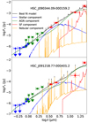 |
Fig. 17. SEDs of BluDOG-like objects. The plots and lines are same as in Figure 3. Arrows denote upper limits. |
5. Conclusions
We have constructed the sample of 74 (65) X-ray detected dust obscured galaxies (DOGs) detected in the 0.5–2 keV bands by the eROSITA/eFEDS survey, and we call them “eFEDS detected DOGs”. Among them, 65 sources have reliable X-ray spectral fits, enabling the investigation of their X-ray properties with a statistically meaningful sample; we refer to these as “eFEDS-DOGs”. The eFEDS-DOGs were identified through a combination of multi-wavelength datasets, including HSC and LS8 optical, VIKING near-infrared (NIR), unWISE mid-infrared (MIR), and eROSITA/eFEDS soft X-ray (0.5–2 keV) bands. Our results are summarized as follows.
-
eFEDS-DOGs occupy a distinct region in the parameter space, with iAB = 22–24 mag and m22 μm = 14–16 mag, previously unexplored by X-ray studies of DOGs.
-
Most DOGs are not detected by eROSITA. Assuming they follow the fiducial L2 − 10 keV(abs, corr)–L6 μm relation of Chen et al. (2017) with a photon index of Γ = 1.8, the expected lower bound of the column density is NH ≳ 1023 cm−2, suggesting that the majority of DOGs are heavily obscured by gas.
-
A large fraction of eFEDS-DOGs show NH ≲ 1022 cm−2, indicating that they are not heavily obscured by gas. This implies that the eFEDS-DOG sample includes DOGs that are unobscured in both gas and dust.
-
Examination of the L6 μm vs. L0.5 − 2 keV(abs, corr) diagram reveals a predominant alignment with the L6 μm–LX relation. However, some eFEDS-DOGs exhibit deviations, down to ≃1.0 dex below the L6 μm–LX relation. Sources located ∼1 dex below the relation may indicate high Eddington ratios, potentially approaching the Eddington limit.
-
25 out of 63 eFEDS-DOGs are located in the forbidden region on the NH vs. λEdd plane, supporting the idea that eFEDS-DOGs in the forbidden region experience gas outflow of the obscuring material, which would eventually lead to a decrease in NH. eFEDS-DOGs are prominent candidates in a previously missed transitional phase between obscured AGNs and optically selected quasars.
-
Despite none of the eFEDS-DOGs meeting the strict BluDOG criteria, our identification of BluDOG-like objects based on
 and MIR_CLASS = 2 (PL DOGs) unveils a compelling subset. Their spectral energy distributions (SEDs) exhibit a power-law trend between the optical and MIR regions, coupled with a distinct flattening between HSC g band and HSC i band. This suggests that these BluDOG-like objects may represent a population of low-redshift BluDOGs.
Data availability
Table A.1 is available at the CDS via https://cdsarc.cds.unistra.fr/viz-bin/cat/J/A+A/702/A34
eROSITA was launched on July 13, 2019.
Acknowledgments
The authors gratefully acknowledge the anonymous referee for a careful reading of the manuscript and very helpful comments. We are honored and grateful for the opportunity to observe the universe from Mauna Kea, which has cultural, historical, and natural significance in Hawaii. The Hyper Suprime-Cam (HSC) Collaboration includes the astronomical communities of Japan, Taiwan, and Princeton University. The HSC instrumentation and software were developed by the National Astronomical Observatory of Japan (NAOJ), the Kavli Institute for the Physics and Mathematics of the Universe (Kavli IPMU), the University of Tokyo, the High Energy Accelerator Research Organization (KEK), the Academia Sinica Institute for Astronomy and Astrophysics in Taiwan (ASIAA), and Princeton University. Funding was contributed by the FIRST program from the Japanese Cabinet Office, the Ministry of Education, Culture, Sports, Science and Technology (MEXT), the Japan Society for the Promotion of Science (JSPS), Japan Science and Technology Agency (JST), the Toray Science Foundation, NAOJ, Kavli IPMU, KEK, ASIAA, and Princeton University. This paper makes use of software developed for the Large Synoptic Survey Telescope. We thank the LSST Project for making their code available as free software at http://dm.lsstcorp.org. The Pan-STARRS1 Surveys (PS1) have been made possible through contributions of the Institute for Astronomy, the University of Hawaii, the Pan-STARRS Project Office, the Max-Planck Society and its participating institutes, the Max Planck Institute for Astronomy, Heidelberg and the Max Planck Institute for Extraterrestrial Physics, Garching, The Johns Hopkins University, Durham University, the University of Edinburgh, Queen’s University Belfast, the Harvard-Smithsonian Center for Astrophysics, the Las Cumbres Observatory Global Telescope Network Incorporated, the National Central University of Taiwan, the Space Telescope Science Institute, the National Aeronautics and Space Administration under Grant No. NNX08AR22G issued through the Planetary Science Division of the NASA Science Mission Directorate, the National Science Foundation under Grant No. AST-1238877, the University of Maryland, and Eotvos Lorand University (ELTE). This publication has made use of data from the VIKING survey from VISTA at the ESO Paranal Observatory, program ID 179.A-2004. Data processing has been contributed by the VISTA Data Flow System at CASU, Cambridge and WFAU, Edinburgh. This publication makes use of data products from the Wide-field Infrared Survey Explorer, which is a joint project of the University of California, Los Angeles, and the Jet Propulsion Laboratory/California Institute of Technology, funded by the National Aeronautics and Space Administration. Herschel is an ESA space observatory with science instruments provided by Europeanled Principal Investigator consortia and with important participation from NASA. The Legacy Surveys consist of three individual and complementary projects: the Dark Energy Camera Legacy Survey (DECaLS; Proposal ID #2014B-0404; PIs: David Schlegel and Arjun Dey), the Beijing-Arizona Sky Survey (BASS; NOAO Prop. ID #2015A-0801; PIs: Zhou Xu and Xiaohui Fan), and the Mayall z-band Legacy Survey (MzLS; Prop. ID #2016A-0453; PI: Arjun Dey). DECaLS, BASS and MzLS together include data obtained, respectively, at the Blanco telescope, Cerro Tololo Inter-American Observatory, NSF’s NOIRLab; the Bok telescope, Steward Observatory, University of Arizona; and the Mayall telescope, Kitt Peak National Observatory, NOIRLab. Pipeline processing and analyses of the data were supported by NOIRLab and the Lawrence Berkeley National Laboratory (LBNL). The Legacy Surveys project is honored to be permitted to conduct astronomical research on Iolkam Du’ag (Kitt Peak), a mountain with particular significance to the Tohono O’odham Nation. NOIRLab is operated by the Association of Universities for Research in Astronomy (AURA) under a cooperative agreement with the National Science Foundation. LBNL is managed by the Regents of the University of California under contract to the U.S. Department of Energy. This project used data obtained with the Dark Energy Camera (DECam), which was constructed by the Dark Energy Survey (DES) collaboration. Funding for the DES Projects has been provided by the U.S. Department of Energy, the U.S. National Science Foundation, the Ministry of Science and Education of Spain, the Science and Technology Facilities Council of the United Kingdom, the Higher Education Funding Council for England, the National Center for Supercomputing Applications at the University of Illinois at Urbana-Champaign, the Kavli Institute of Cosmological Physics at the University of Chicago, Center for Cosmology and Astro-Particle Physics at the Ohio State University, the Mitchell Institute for Fundamental Physics and Astronomy at Texas A&M University, Financiadora de Estudos e Projetos, Fundacao Carlos Chagas Filho de Amparo, Financiadora de Estudos e Projetos, Fundacao Carlos Chagas Filho de Amparo a Pesquisa do Estado do Rio de Janeiro, Conselho Nacional de Desenvolvimento Cientifico e Tecnologico and the Ministerio da Ciencia, Tecnologia e Inovacao, the Deutsche Forschungsgemeinschaft and the Collaborating Institutions in the Dark Energy Survey. The Collaborating Institutions are Argonne National Laboratory, the University of California at Santa Cruz, the University of Cambridge, Centro de Investigaciones Energeticas, Medioambientales y Tecnologicas-Madrid, the University of Chicago, University College London, the DES-Brazil Consortium, the University of Edinburgh, the Eidgenossische Technische Hochschule (ETH) Zurich, Fermi National Accelerator Laboratory, the University of Illinois at Urbana-Champaign, the Institut de Ciencies de l’Espai (IEEC/CSIC), the Institut de Fisica d’Altes Energies, Lawrence Berkeley National Laboratory, the Ludwig Maximilians Universitat Munchen and the associated Excellence Cluster Universe, the University of Michigan, NSF’s NOIRLab, the University of Nottingham, the Ohio State University, the University of Pennsylvania, the University of Portsmouth, SLAC National Accelerator Laboratory, Stanford University, the University of Sussex, and Texas A&M University. BASS is a key project of the Telescope Access Program (TAP), which has been funded by the National Astronomical Observatories of China, the Chinese Academy of Sciences (the Strategic Priority Research Program “The Emergence of Cosmological Structures” Grant # XDB09000000), and the Special Fund for Astronomy from the Ministry of Finance. The BASS is also supported by the External Cooperation Program of Chinese Academy of Sciences (Grant # 114A11KYSB20160057), and Chinese National Natural Science Foundation (Grant # 12120101003, # 11433005). The Legacy Survey team makes use of data products from the Near-Earth Object Wide-field Infrared Survey Explorer (NEOWISE), which is a project of the Jet Propulsion Laboratory/California Institute of Technology. NEOWISE is funded by the National Aeronautics and Space Administration. The Legacy Surveys imaging of the DESI footprint is supported by the Director, Office of Science, Office of High Energy Physics of the U.S. Department of Energy under Contract No. DE-AC02-05CH1123, by the National Energy Research Scientific Computing Center, a DOE Office of Science User Facility under the same contract; and by the U.S. National Science Foundation, Division of Astronomical Sciences under Contract No. AST-0950945 to NOAO. This work is based on data from eROSITA, the soft X-ray instrument aboard SRG, a joint Russian-German science mission supported by the Russian Space Agency (Roskosmos), in the interests of the Russian Academy of Sciences represented by its Space Research Institute (IKI), and the Deutsches Zentrum für Luftund Raumfahrt (DLR). The SRG spacecraft was built by Lavochkin Association (NPOL) and its subcontractors, and is operated by NPOL with support from the Max Planck Institute for Extraterrestrial Physics (MPE). The development and construction of the eROSITA X-ray instrument was led by MPE, with contributions from the Dr. Karl Remeis Observatory Bamberg & ECAP (FAU Erlangen-Nuernberg), the University of Hamburg Observatory, the Leibniz Institute for Astrophysics Potsdam (AIP), and the Institute for Astronomy and Astrophysics of the University of Tübingen, with the support of DLR and the Max Planck Society. The Argelander Institute for Astronomy of the University of Bonn and the Ludwig Maximilians Universität Munich also participated in the science preparation for eROSITA. This research made use of Astropy (https://www.astropy.org) a community-developed core Python package for Astronomy (Astropy Collaboration 2013, 2018, 2022). This study was financially supported by the Japan Society for the Promotion of Science (JSPS) KAKENHI grant Nos. 20H01939 and 25K01043 (K.I.). K.I. also acknowledges support from the Inamori Research Grants, which helped make this research possible.
References
- Abazajian, K., Adelman-McCarthy, J. K., Agüeros, M. A., et al. 2004, AJ, 128, 502 [NASA ADS] [CrossRef] [Google Scholar]
- Abramowicz, M. A., Czerny, B., Lasota, J. P., & Szuszkiewicz, E. 1988, ApJ, 332, 646 [Google Scholar]
- Aihara, H., Arimoto, N., Armstrong, R., et al. 2018a, PASJ, 70, S4 [NASA ADS] [Google Scholar]
- Aihara, H., Armstrong, R., Bickerton, S., et al. 2018b, PASJ, 70, S8 [NASA ADS] [Google Scholar]
- Aihara, H., AlSayyad, Y., Ando, M., et al. 2019, PASJ, 71, 114 [Google Scholar]
- Akins, H. B., Casey, C. M., Allen, N., et al. 2023, ApJ, 956, 61 [NASA ADS] [CrossRef] [Google Scholar]
- Aller, M. C., & Richstone, D. O. 2007, ApJ, 665, 120 [Google Scholar]
- Almeida, A., Anderson, S. F., Argudo-Fernández, M., et al. 2023, ApJS, 267, 44 [NASA ADS] [CrossRef] [Google Scholar]
- Alonso-Herrero, A., Pérez-González, P. G., Alexander, D. M., et al. 2006, ApJ, 640, 167 [Google Scholar]
- Arnaboldi, M., Neeser, M. J., Parker, L. C., et al. 2007, The Messenger, 127, 28 [NASA ADS] [Google Scholar]
- Arnaud, K. A. 1996, ASP Conf. Ser., 101, 17 [Google Scholar]
- Arnouts, S., Cristiani, S., Moscardini, L., et al. 1999, MNRAS, 310, 540 [Google Scholar]
- Asmus, D., Gandhi, P., Hönig, S. F., Smette, A., & Duschl, W. J. 2015, MNRAS, 454, 766 [NASA ADS] [CrossRef] [Google Scholar]
- Assef, R. J., Walton, D. J., Brightman, M., et al. 2016, ApJ, 819, 111 [Google Scholar]
- Assef, R. J., Brightman, M., Walton, D. J., et al. 2020, ApJ, 897, 112 [NASA ADS] [CrossRef] [Google Scholar]
- Astropy Collaboration (Robitaille, T. P., et al.) 2013, A&A, 558, A33 [NASA ADS] [CrossRef] [EDP Sciences] [Google Scholar]
- Astropy Collaboration (Price-Whelan, A. M., et al.) 2018, AJ, 156, 123 [Google Scholar]
- Astropy Collaboration (Price-Whelan, A. M., et al.) 2022, ApJ, 935, 167 [NASA ADS] [CrossRef] [Google Scholar]
- Axelrod, T., Kantor, J., Lupton, R. H., & Pierfederici, F. 2010, Proc. SPIE, 7740, 774015 [Google Scholar]
- Barro, G., Pérez-González, P. G., Kocevski, D. D., et al. 2024, ApJ, 963, 128 [CrossRef] [Google Scholar]
- Becker, R. H., White, R. L., & Helfand, D. J. 1995, ApJ, 450, 559 [Google Scholar]
- Boller, T., Brandt, W. N., & Fink, H. 1996, A&A, 305, 53 [NASA ADS] [Google Scholar]
- Boquien, M., Burgarella, D., Roehlly, Y., et al. 2019, A&A, 622, A103 [NASA ADS] [CrossRef] [EDP Sciences] [Google Scholar]
- Bosch, J., Armstrong, R., Bickerton, S., et al. 2018, PASJ, 70, S5 [Google Scholar]
- Brightman, M., Silverman, J. D., Mainieri, V., et al. 2013, MNRAS, 433, 2485 [Google Scholar]
- Brunner, H., Liu, T., Lamer, G., et al. 2022, A&A, 661, A1 [NASA ADS] [CrossRef] [EDP Sciences] [Google Scholar]
- Bruzual, G., & Charlot, S. 2003, MNRAS, 344, 1000 [NASA ADS] [CrossRef] [Google Scholar]
- Buchner, J. 2021, J Open Source Software, 6, 3045 [Google Scholar]
- Buchner, J., Georgakakis, A., Nandra, K., et al. 2014, A&A, 564, A125 [NASA ADS] [CrossRef] [EDP Sciences] [Google Scholar]
- Burgarella, D., Buat, V., & Iglesias-Páramo, J. 2005, MNRAS, 360, 1413 [NASA ADS] [CrossRef] [Google Scholar]
- Bussmann, R. S., Dey, A., Borys, C., et al. 2009a, ApJ, 705, 184 [NASA ADS] [CrossRef] [Google Scholar]
- Bussmann, R. S., Dey, A., Lotz, J., et al. 2009b, ApJ, 693, 750 [Google Scholar]
- Bussmann, R. S., Dey, A., Lotz, J., et al. 2011, ApJ, 733, 21 [NASA ADS] [CrossRef] [Google Scholar]
- Calzetti, D., Armus, L., Bohlin, R. C., et al. 2000, ApJ, 533, 682 [NASA ADS] [CrossRef] [Google Scholar]
- Cardelli, J. A., Clayton, G. C., & Mathis, J. S. 1989, ApJ, 345, 245 [Google Scholar]
- Chabrier, G. 2003, PASP, 115, 763 [Google Scholar]
- Chan, J. H. H., Wong, K. C., Ding, X., et al. 2024, MNRAS, 527, 6253 [Google Scholar]
- Chen, C.-T. J., Hickox, R. C., Goulding, A. D., et al. 2017, ApJ, 837, 145 [Google Scholar]
- Chen, C. T. J., Brandt, W. N., Luo, B., et al. 2018, MNRAS, 478, 2132 [NASA ADS] [CrossRef] [Google Scholar]
- Ciesla, L., Charmandaris, V., Georgakakis, A., et al. 2015, A&A, 576, A10 [NASA ADS] [CrossRef] [EDP Sciences] [Google Scholar]
- Connor, T., Stern, D., Bañados, E., & Mazzucchelli, C. 2021, ApJ, 922, L24 [Google Scholar]
- Corral, A., Georgantopoulos, I., Comastri, A., et al. 2016, A&A, 592, A109 [NASA ADS] [CrossRef] [EDP Sciences] [Google Scholar]
- Cross, N. J. G., Collins, R. S., Mann, R. G., et al. 2012, A&A, 548, A119 [NASA ADS] [CrossRef] [EDP Sciences] [Google Scholar]
- Cutri, R. M. 2014, VizieR Online Data Catalog: II/328 [Google Scholar]
- Cutri, R. M., Wright, E. L., Conrow, T., et al. 2013, Explanatory Supplement to the AllWISE Data Release Products [Google Scholar]
- Dai, X., Kochanek, C. S., Chartas, G., et al. 2010, ApJ, 709, 278 [Google Scholar]
- Dale, D. A., Helou, G., Magdis, G. E., et al. 2014, ApJ, 784, 83 [Google Scholar]
- Dalton, G. B., Caldwell, M., Ward, A. K., et al. 2006, Proc. SPIE, 6269, 62690X [Google Scholar]
- Davies, R. I., Müller Sánchez, F., Genzel, R., et al. 2007, ApJ, 671, 1388 [Google Scholar]
- Davies, R. I., Burtscher, L., Rosario, D., et al. 2015, ApJ, 806, 127 [Google Scholar]
- Desai, V., Soifer, B. T., Dey, A., et al. 2009, ApJ, 700, 1190 [NASA ADS] [CrossRef] [Google Scholar]
- Dey, A., Soifer, B. T., Desai, V., et al. 2008, ApJ, 677, 943 [NASA ADS] [CrossRef] [Google Scholar]
- Dey, A., Schlegel, D. J., Lang, D., et al. 2019, AJ, 157, 168 [Google Scholar]
- Díaz-Santos, T., Assef, R. J., Eisenhardt, P. R. M., et al. 2021, A&A, 654, A37 [NASA ADS] [CrossRef] [EDP Sciences] [Google Scholar]
- Ding, X., Silverman, J., Treu, T., et al. 2020, ApJ, 888, 37 [NASA ADS] [CrossRef] [Google Scholar]
- Eisenhardt, P. R. M., Wu, J., Tsai, C.-W., et al. 2012, ApJ, 755, 173 [Google Scholar]
- Fabian, A. C., Celotti, A., & Erlund, M. C. 2006, MNRAS, 373, L16 [NASA ADS] [Google Scholar]
- Fabian, A. C., Vasudevan, R. V., Mushotzky, R. F., Winter, L. M., & Reynolds, C. S. 2009, MNRAS, 394, L89 [NASA ADS] [CrossRef] [Google Scholar]
- Fan, X., Wang, F., Yang, J., et al. 2019, ApJ, 870, L11 [Google Scholar]
- Ferrarese, L., & Merritt, D. 2000, ApJ, 539, L9 [Google Scholar]
- Fiore, F., Grazian, A., Santini, P., et al. 2008, ApJ, 672, 94 [NASA ADS] [CrossRef] [Google Scholar]
- Fujimoto, S., Oguri, M., Nagao, T., Izumi, T., & Ouchi, M. 2020, ApJ, 891, 64 [NASA ADS] [CrossRef] [Google Scholar]
- Fukuchi, H., Ichikawa, K., Akiyama, M., et al. 2025, ApJ, 987, 66 [Google Scholar]
- Furtak, L. J., Zitrin, A., Plat, A., et al. 2023, ApJ, 952, 142 [NASA ADS] [CrossRef] [Google Scholar]
- Furtak, L. J., Labbé, I., Zitrin, A., et al. 2024, Nature, 628, 57 [NASA ADS] [CrossRef] [Google Scholar]
- Furusawa, H., Koike, M., Takata, T., et al. 2018, PASJ, 70, S3 [Google Scholar]
- Gandhi, P., Horst, H., Smette, A., et al. 2009, A&A, 502, 457 [NASA ADS] [CrossRef] [EDP Sciences] [Google Scholar]
- Gandhi, P., Hönig, S. F., & Kishimoto, M. 2015, ApJ, 812, 113 [NASA ADS] [CrossRef] [Google Scholar]
- Gebhardt, K., Bender, R., Bower, G., et al. 2000, ApJ, 539, L13 [Google Scholar]
- Ghisellini, G., Righi, C., Costamante, L., & Tavecchio, F. 2017, MNRAS, 469, 255 [NASA ADS] [CrossRef] [Google Scholar]
- Gilli, R., Comastri, A., & Hasinger, G. 2007, A&A, 463, 79 [NASA ADS] [CrossRef] [EDP Sciences] [Google Scholar]
- Glikman, E., Rusu, C. E., Djorgovski, S. G., et al. 2018, ArXiv e-prints [arXiv:1807.05434] [Google Scholar]
- Goulding, A. D., Greene, J. E., Bezanson, R., et al. 2018, PASJ, 70, S37 [NASA ADS] [CrossRef] [Google Scholar]
- Helfand, D. J., White, R. L., & Becker, R. H. 2015, ApJ, 801, 26 [NASA ADS] [CrossRef] [Google Scholar]
- HI4PI Collaboration (Ben Bekhti, N., et al.) 2016, A&A, 594, A116 [NASA ADS] [CrossRef] [EDP Sciences] [Google Scholar]
- Hopkins, P. F., Hernquist, L., Cox, T. J., & Kereš, D. 2008, ApJS, 175, 356 [Google Scholar]
- Ichikawa, K., Ueda, Y., Terashima, Y., et al. 2012, ApJ, 754, 45 [Google Scholar]
- Ichikawa, K., Imanishi, M., Ueda, Y., et al. 2014, ApJ, 794, 139 [Google Scholar]
- Ichikawa, K., Ricci, C., Ueda, Y., et al. 2017, ApJ, 835, 74 [NASA ADS] [CrossRef] [Google Scholar]
- Ichikawa, K., Ricci, C., Ueda, Y., et al. 2019a, ApJ, 870, 31 [NASA ADS] [CrossRef] [Google Scholar]
- Ichikawa, K., Ueda, J., Bae, H.-J., et al. 2019b, ApJ, 870, 65 [NASA ADS] [CrossRef] [Google Scholar]
- Ichikawa, K., Yamashita, T., Merloni, A., et al. 2023, A&A, 672, A171 [NASA ADS] [CrossRef] [EDP Sciences] [Google Scholar]
- Ighina, L., Caccianiga, A., Moretti, A., et al. 2019, MNRAS, 489, 2732 [NASA ADS] [CrossRef] [Google Scholar]
- Ilbert, O., Arnouts, S., McCracken, H. J., et al. 2006, A&A, 457, 841 [NASA ADS] [CrossRef] [EDP Sciences] [Google Scholar]
- Inayoshi, K., Haiman, Z., & Ostriker, J. P. 2016, MNRAS, 459, 3738 [NASA ADS] [CrossRef] [Google Scholar]
- Inayoshi, K., Visbal, E., & Haiman, Z. 2020, ARA&A, 58, 27 [NASA ADS] [CrossRef] [Google Scholar]
- Inoue, A. K. 2011, MNRAS, 415, 2920 [NASA ADS] [CrossRef] [Google Scholar]
- Ishibashi, W., & Courvoisier, T. J. L. 2010, A&A, 512, A58 [NASA ADS] [CrossRef] [EDP Sciences] [Google Scholar]
- Ishibashi, W., Fabian, A. C., Ricci, C., & Celotti, A. 2018, MNRAS, 479, 3335 [CrossRef] [Google Scholar]
- Ishida, C. M. 2004, Ph.D. Thesis, University of Hawaii, Manoa [Google Scholar]
- Ivezić, Ž., Kahn, S. M., Tyson, J. A., et al. 2019, ApJ, 873, 111 [Google Scholar]
- Jansen, F., Lumb, D., Altieri, B., et al. 2001, A&A, 365, L1 [NASA ADS] [CrossRef] [EDP Sciences] [Google Scholar]
- Just, D. W., Brandt, W. N., Shemmer, O., et al. 2007, ApJ, 665, 1004 [Google Scholar]
- Kartaltepe, J. S., Sanders, D. B., Le Floc’h, E., et al. 2010, ApJ, 721, 98 [NASA ADS] [CrossRef] [Google Scholar]
- Kato, S., Fukue, J., & Mineshige, S. 2008, Black-Hole Accretion Disks – Towards a New Paradigm [Google Scholar]
- Kawanomoto, S., Uraguchi, F., Komiyama, Y., et al. 2018, PASJ, 70, 66 [Google Scholar]
- Kayal, A., & Singh, V. 2024, MNRAS, 531, 830 [Google Scholar]
- Kocevski, D. D., Onoue, M., Inayoshi, K., et al. 2023, ApJ, 954, L4 [NASA ADS] [CrossRef] [Google Scholar]
- Kocevski, D. D., Finkelstein, S. L., Barro, G., et al. 2024, ArXiv e-prints [arXiv:2404.03576] [Google Scholar]
- Kokorev, V., Fujimoto, S., Labbe, I., et al. 2023, ApJ, 957, L7 [NASA ADS] [CrossRef] [Google Scholar]
- Kollmeier, J. A., Onken, C. A., Kochanek, C. S., et al. 2006, ApJ, 648, 128 [NASA ADS] [CrossRef] [Google Scholar]
- Komiyama, Y., Obuchi, Y., Nakaya, H., et al. 2018, PASJ, 70, S2 [Google Scholar]
- Kormendy, J., & Ho, L. C. 2013, ARA&A, 51, 511 [Google Scholar]
- Labbe, I., Greene, J. E., Bezanson, R., et al. 2025, ApJ, 978, 92 [NASA ADS] [CrossRef] [Google Scholar]
- Lacy, M., Baum, S. A., Chandler, C. J., et al. 2020, PASP, 132, 035001 [Google Scholar]
- Lang, D. 2014, AJ, 147, 108 [Google Scholar]
- Lang, D., Hogg, D. W., & Schlegel, D. J. 2016, AJ, 151, 36 [Google Scholar]
- Lanzuisi, G., Piconcelli, E., Fiore, F., et al. 2009, A&A, 498, 67 [NASA ADS] [CrossRef] [EDP Sciences] [Google Scholar]
- Leitherer, C., Li, I. H., Calzetti, D., & Heckman, T. M. 2002, ApJS, 140, 303 [NASA ADS] [CrossRef] [Google Scholar]
- Liu, T., Buchner, J., Nandra, K., et al. 2022, A&A, 661, A5 [NASA ADS] [CrossRef] [EDP Sciences] [Google Scholar]
- Lonsdale, C. J., Smith, H. E., Rowan-Robinson, M., et al. 2003, PASP, 115, 897 [Google Scholar]
- LSST Science Collaboration (Abell, P. A., et al.) 2009, ArXiv e-prints [arXiv:0912.0201] [Google Scholar]
- Lupton, R., Gunn, J. E., Ivezić, Z., Knapp, G. R., & Kent, S. 2001, ASP Conf. Ser., 238, 269 [NASA ADS] [Google Scholar]
- Lyu, J., & Rieke, G. 2022, Universe, 8, 304 [Google Scholar]
- Magorrian, J., Tremaine, S., Richstone, D., et al. 1998, AJ, 115, 2285 [Google Scholar]
- Mainzer, A., Bauer, J., Cutri, R. M., et al. 2014, ApJ, 792, 30 [Google Scholar]
- Maiolino, R., Risaliti, G., Salvati, M., et al. 2010, A&A, 517, A47 [NASA ADS] [CrossRef] [EDP Sciences] [Google Scholar]
- Marconi, A., & Hunt, L. K. 2003, ApJ, 589, L21 [Google Scholar]
- Markowitz, A. G., Krumpe, M., & Nikutta, R. 2014, MNRAS, 439, 1403 [Google Scholar]
- Mateos, S., Carrera, F. J., Alonso-Herrero, A., et al. 2015, MNRAS, 449, 1422 [Google Scholar]
- Matsuoka, K., Nagao, T., Maiolino, R., et al. 2017, A&A, 608, A90 [NASA ADS] [CrossRef] [EDP Sciences] [Google Scholar]
- Matsuta, K., Gandhi, P., Dotani, T., et al. 2012, ApJ, 753, 104 [NASA ADS] [CrossRef] [Google Scholar]
- Matthee, J., Naidu, R. P., Brammer, G., et al. 2024, ApJ, 963, 129 [NASA ADS] [CrossRef] [Google Scholar]
- McKinney, J. C., Tchekhovskoy, A., Sadowski, A., & Narayan, R. 2014, MNRAS, 441, 3177 [NASA ADS] [CrossRef] [Google Scholar]
- Melbourne, J., Bussman, R. S., Brand, K., et al. 2009, AJ, 137, 4854 [Google Scholar]
- Melbourne, J., Peng, C. Y., Soifer, B. T., et al. 2011, AJ, 141, 141 [Google Scholar]
- Melbourne, J., Soifer, B. T., Desai, V., et al. 2012, AJ, 143, 125 [Google Scholar]
- Merloni, A., Nandra, K., & Predehl, P. 2020, Nat. Astron., 4, 634 [Google Scholar]
- Merloni, A., Lamer, G., Liu, T., et al. 2024, A&A, 682, A34 [NASA ADS] [CrossRef] [EDP Sciences] [Google Scholar]
- Miller, B. P., Brandt, W. N., Schneider, D. P., et al. 2011, ApJ, 726, 20 [Google Scholar]
- Minezaki, T., & Matsushita, K. 2015, ApJ, 802, 98 [NASA ADS] [CrossRef] [Google Scholar]
- Miyazaki, S., Komiyama, Y., Kawanomoto, S., et al. 2018, PASJ, 70, S1 [NASA ADS] [Google Scholar]
- Morgan, C. W., Kochanek, C. S., Morgan, N. D., & Falco, E. E. 2010, ApJ, 712, 1129 [Google Scholar]
- Nandra, K., Waddell, S. G. H., Liu, T., et al. 2025, A&A, 693, A212 [NASA ADS] [CrossRef] [EDP Sciences] [Google Scholar]
- Nanni, R., Vignali, C., Gilli, R., Moretti, A., & Brandt, W. N. 2017, A&A, 603, A128 [NASA ADS] [CrossRef] [EDP Sciences] [Google Scholar]
- Ni, Q., Brandt, W. N., Chen, C.-T., et al. 2021, ApJS, 256, 21 [CrossRef] [Google Scholar]
- Noboriguchi, A., Nagao, T., Toba, Y., et al. 2019, ApJ, 876, 132 [NASA ADS] [CrossRef] [Google Scholar]
- Noboriguchi, A., Nagao, T., Toba, Y., et al. 2022, ApJ, 941, 195 [Google Scholar]
- Noboriguchi, A., Inoue, A. K., Nagao, T., Toba, Y., & Misawa, T. 2023, ApJ, 959, L14 [Google Scholar]
- Noll, S., Burgarella, D., Giovannoli, E., et al. 2009, A&A, 507, 1793 [NASA ADS] [CrossRef] [EDP Sciences] [Google Scholar]
- Ohsuga, K., Mori, M., Nakamoto, T., & Mineshige, S. 2005, ApJ, 628, 368 [NASA ADS] [CrossRef] [Google Scholar]
- Ohsuga, K., Mineshige, S., Mori, M., & Kato, Y. 2009, PASJ, 61, L7 [NASA ADS] [Google Scholar]
- Pacaud, F., Pierre, M., Refregier, A., et al. 2006, MNRAS, 372, 578 [NASA ADS] [CrossRef] [Google Scholar]
- Perrotta, S., Hamann, F., Zakamska, N. L., et al. 2019, MNRAS, 488, 4126 [Google Scholar]
- Piconcelli, E., Jimenez-Bailón, E., Guainazzi, M., et al. 2005, A&A, 432, 15 [NASA ADS] [CrossRef] [EDP Sciences] [Google Scholar]
- Pierre, M., Pacaud, F., Adami, C., et al. 2016, A&A, 592, A1 [NASA ADS] [CrossRef] [EDP Sciences] [Google Scholar]
- Predehl, P., Andritschke, R., Arefiev, V., et al. 2021, A&A, 647, A1 [EDP Sciences] [Google Scholar]
- Ricci, C., Assef, R. J., Stern, D., et al. 2017a, ApJ, 835, 105 [Google Scholar]
- Ricci, C., Trakhtenbrot, B., Koss, M. J., et al. 2017b, Nature, 549, 488 [NASA ADS] [CrossRef] [Google Scholar]
- Ricci, C., Ananna, T. T., Temple, M. J., et al. 2022, ApJ, 938, 67 [NASA ADS] [CrossRef] [Google Scholar]
- Ricci, C., Ichikawa, K., Stalevski, M., et al. 2023, ApJ, 959, 27 [NASA ADS] [CrossRef] [Google Scholar]
- Riguccini, L. A., Treister, E., Menéndez-Delmestre, K., et al. 2019, AJ, 157, 233 [NASA ADS] [CrossRef] [Google Scholar]
- Risaliti, G., Elvis, M., Fabbiano, G., et al. 2007, ApJ, 659, L111 [NASA ADS] [CrossRef] [Google Scholar]
- Risaliti, G., Young, M., & Elvis, M. 2009, ApJ, 700, L6 [NASA ADS] [CrossRef] [Google Scholar]
- Risaliti, G., Nardini, E., Salvati, M., et al. 2011, MNRAS, 410, 1027 [Google Scholar]
- Salvato, M., Wolf, J., Dwelly, T., et al. 2022, A&A, 661, A3 [NASA ADS] [CrossRef] [EDP Sciences] [Google Scholar]
- Sanders, D. B., Soifer, B. T., Elias, J. H., et al. 1988, ApJ, 325, 74 [Google Scholar]
- Sawicki, M. 2002, AJ, 124, 3050 [Google Scholar]
- Schlafly, E. F., Meisner, A. M., & Green, G. M. 2019, ApJS, 240, 30 [Google Scholar]
- Schlegel, D. J., Finkbeiner, D. P., & Davis, M. 1998, ApJ, 500, 525 [Google Scholar]
- Shemmer, O., Brandt, W. N., Schneider, D. P., et al. 2006, ApJ, 644, 86 [NASA ADS] [CrossRef] [Google Scholar]
- Shemmer, O., Brandt, W. N., Netzer, H., Maiolino, R., & Kaspi, S. 2008, ApJ, 682, 81 [Google Scholar]
- Shen, Y., Richards, G. T., Strauss, M. A., et al. 2011, ApJS, 194, 45 [Google Scholar]
- Stalevski, M., Ricci, C., Ueda, Y., et al. 2016, MNRAS, 458, 2288 [Google Scholar]
- Stern, D. 2015, ApJ, 807, 129 [Google Scholar]
- Stern, D., Lansbury, G. B., Assef, R. J., et al. 2014, ApJ, 794, 102 [Google Scholar]
- Suleiman, N., Noboriguchi, A., Toba, Y., et al. 2022, PASJ, 74, 1157 [NASA ADS] [CrossRef] [Google Scholar]
- Sunyaev, R., Arefiev, V., Babyshkin, V., et al. 2021, A&A, 656, A132 [NASA ADS] [CrossRef] [EDP Sciences] [Google Scholar]
- Takeo, E., Inayoshi, K., & Mineshige, S. 2020, MNRAS, 497, 302 [NASA ADS] [CrossRef] [Google Scholar]
- Titarchuk, L., & Lyubarskij, Y. 1995, ApJ, 450, 876 [NASA ADS] [CrossRef] [Google Scholar]
- Toba, Y., & Nagao, T. 2016, ApJ, 820, 46 [Google Scholar]
- Toba, Y., Nagao, T., Strauss, M. A., et al. 2015, PASJ, 67, 86 [Google Scholar]
- Toba, Y., Nagao, T., Kajisawa, M., et al. 2017, ApJ, 835, 36 [NASA ADS] [CrossRef] [Google Scholar]
- Toba, Y., Ueda, Y., Matsuoka, K., et al. 2019, MNRAS, 484, 196 [Google Scholar]
- Toba, Y., Yamada, S., Ueda, Y., et al. 2020, ApJ, 888, 8 [Google Scholar]
- Toba, Y., Liu, T., Urrutia, T., et al. 2022, A&A, 661, A15 [NASA ADS] [CrossRef] [EDP Sciences] [Google Scholar]
- Trakhtenbrot, B., Ricci, C., Koss, M. J., et al. 2017, MNRAS, 470, 800 [NASA ADS] [CrossRef] [Google Scholar]
- Treister, E., Schawinski, K., Urry, C. M., & Simmons, B. D. 2012, ApJ, 758, L39 [NASA ADS] [CrossRef] [Google Scholar]
- Tremaine, S., Gebhardt, K., Bender, R., et al. 2002, ApJ, 574, 740 [NASA ADS] [CrossRef] [Google Scholar]
- Veilleux, S., Kim, D. C., & Sanders, D. B. 2002, ApJS, 143, 315 [NASA ADS] [CrossRef] [Google Scholar]
- Vietri, G., Piconcelli, E., Bischetti, M., et al. 2018, A&A, 617, A81 [NASA ADS] [CrossRef] [EDP Sciences] [Google Scholar]
- Vignali, C., Brandt, W. N., Schneider, D. P., & Kaspi, S. 2005, AJ, 129, 2519 [NASA ADS] [CrossRef] [Google Scholar]
- Vito, F., Brandt, W. N., Stern, D., et al. 2018, MNRAS, 474, 4528 [Google Scholar]
- Vito, F., Brandt, W. N., Bauer, F. E., et al. 2019, A&A, 630, A118 [NASA ADS] [CrossRef] [EDP Sciences] [Google Scholar]
- Wang, F., Fan, X., Yang, J., et al. 2021, ApJ, 908, 53 [Google Scholar]
- White, R. L., Becker, R. H., Helfand, D. J., & Gregg, M. D. 1997, ApJ, 475, 479 [Google Scholar]
- Wright, E. L., Eisenhardt, P. R. M., Mainzer, A. K., et al. 2010, AJ, 140, 1868 [Google Scholar]
- Wu, J., Brandt, W. N., Miller, B. P., et al. 2013, ApJ, 763, 109 [NASA ADS] [CrossRef] [Google Scholar]
- Wu, J., Jun, H. D., Assef, R. J., et al. 2018, ApJ, 852, 96 [NASA ADS] [CrossRef] [Google Scholar]
- Yamada, S., Ueda, Y., Tanimoto, A., et al. 2021, ApJS, 257, 61 [NASA ADS] [CrossRef] [Google Scholar]
- Yamada, S., Ueda, Y., Herrera-Endoqui, M., et al. 2023, ApJS, 265, 37 [NASA ADS] [CrossRef] [Google Scholar]
- Yang, G., Boquien, M., Brandt, W. N., et al. 2022, ApJ, 927, 192 [NASA ADS] [CrossRef] [Google Scholar]
- Yoshida, T., Nagao, T., Toba, Y., et al. 2025, ApJ, 987, 141 [Google Scholar]
- Yu, Z., Brandt, W. N., Zou, F., et al. 2024, ApJ, 977, 210 [Google Scholar]
- Yue, M., Eilers, A.-C., Ananna, T. T., et al. 2024, ApJ, 974, L26 [CrossRef] [Google Scholar]
- Yutani, N., Toba, Y., Baba, S., & Wada, K. 2022, ApJ, 936, 118 [NASA ADS] [CrossRef] [Google Scholar]
- Zappacosta, L., Piconcelli, E., Duras, F., et al. 2018, A&A, 618, A28 [NASA ADS] [CrossRef] [EDP Sciences] [Google Scholar]
- Zdziarski, A. A., Johnson, W. N., & Magdziarz, P. 1996, MNRAS, 283, 193 [NASA ADS] [CrossRef] [Google Scholar]
- Zhu, S. F., Brandt, W. N., Luo, B., et al. 2020, MNRAS, 496, 245 [Google Scholar]
- Zou, F., Brandt, W. N., Vito, F., et al. 2020, MNRAS, 499, 1823 [NASA ADS] [CrossRef] [Google Scholar]
Appendix A: eFEDS-DOG catalog information
In Table A.1, we provide a list of column names for our eFEDS-DOG catalogs. These catalogs encompass a range of photometric data, including ID, R.A., Dec., magnitudes in each band, optical spectral index, MIR and optical classification, observed flux between 0.5–2 keV, absorption-corrected intrinsic luminosity between 0.5–2 keV, redshift, redshift grade, absorption non-corrected luminosity between 0.5–2 keV, hydrogen column density, monochromatic luminosity at rest-frame 6 μm, and photon index. Additionally, the catalog includes information on errors, upper and lower flags associated with each parameter.
The eFEDS-DOG samples were meticulously selected through the combination of catalogs utilizing HSC, VIKING, unWISE, and the eFEDS clean sample (refer to Section 2.1). In total, the catalog comprises 65 eFEDS-DOGs, providing a comprehensive dataset for further analysis.
Column name, units and description of the our eFEDS-DOG catalogs.
Appendix B: Parameters for CIGALE fitting
To decompose the L6μm of the AGN from the total L6μm, we employ the Code Investigating GAlaxy Emission (CIGALE, version 2022.1; Burgarella et al. 2005; Noll et al. 2009; Boquien et al. 2019). CIGALE performs spectral energy distribution (SED) fitting in a self-consistent framework, balancing UV/optical absorption and IR emission.
We adopt a delayed star formation history (SFH; Ciesla et al. 2015), parameterized by the e-folding times of the main stellar population (τmain) and late starburst population (τburst), the mass fraction of the late burst population (fburst), and the ages of the main stellar population (Agemain) and the late burst population (Ageburst). For the stellar population, we assume the initial mass function of Chabrier (2003), solar metallicity, and a 10 Gyr separation between young and old stellar populations (Ageseparation).
The nebular emission model from Inoue (2011) is characterized by the ionization parameter (U), the fraction of Lyman continuum photons escaping the galaxy (fesc), the fraction absorbed by dust (fdust), and the line width. Dust attenuation is modeled using the modified approach presented in Boquien et al. (2019). The attenuation for the continuum follows the model by Calzetti et al. (2000), with extensions by Leitherer et al. (2002) for wavelengths between the Lyman break and 1500 Å. Emission lines are attenuated using a Milky Way extinction law with RV = 3.1 (Cardelli et al. 1989), and we adopt E(B − V)continuum = 0.44E(B − V)line as suggested by Calzetti et al. (2000).
For the AGN emission, we utilize the SKIRTOR model, which incorporates geometric parameters of the AGN and accounts for extinction by polar dust. The parameters include the average edge-on optical depth at 9.7 μm (τ9.7), torus density parameters (p and q; Stalevski et al. (2016)), the opening angle of the torus (oa), the ratio of the maximum to minimum radii of the torus (Rratio), the fraction of dust mass inside clumps (Mcl), the inclination angle (i), the AGN fraction (fAGN), the extinction law, the color excess of the polar dust ( ), the dust temperature (
 ), and the emissivity index of the polar dust.
For BluDOG-like objects, the observed magnitudes in the g and r bands are treated as upper limits to account for the effects of broad emission lines with large equivalent widths (Noboriguchi et al. 2022). In the SED fitting of these BluDOGs, we use the parameter set described in Table 8 of Noboriguchi et al. (2022). For eFEDS-DOGs without BluDOG-like objects, we utilize a parameter set shown in Table B.1.
Appendix C: Criteria of upper-limit of L6 μm
To estimate L6μm for each detection case and redshift, we classified eFEDS-DOGs according to the categories outlined in Table C.1. Additionally, we summarize the criteria for the upper limit of L6 μm.
(1) For objects with detections in the W2, W3, and W4 bands, we fit their MIR SEDs using a power-law function. Out of the 65 eFEDS-DOGs, 44 sources are detected in all three MIR bands. We estimate L6 μm from the best-fit power-law function, and no upper flag is assigned to L6 μm.
(2) One eFEDS-DOG shows non-detection only in the W2 band. For this source, we extrapolate the flux density at rest-frame 6 μm (f6 μm) using a power-law extrapolation from the slope between W3 and W4. Since the extrapolated flux density at W2 ( ) is fainter than the limiting flux density at W2 (
 ), no upper flag is assigned to L6 μm.
(3) Out of 65 sources, 18 eFEDS-DOGs were undetected in the W3 band. Among them, three show that their estimated W3 band fluxes ( ), interpolated by W2 and W4 bands fluxes, are fainter than the W3 band limiting flux (
 ). In this case, we estimate f6 μm using a power-law interpolation between W2 and W4, and no upper flag is assigned to L6 μm.
(4) For the remaining 15 eFEDS-DOGs undetected in the W3 band, the simple interpolation between W2 and W4 results in  . In this case, we use
  to estimate f6 μm, employing a power-law interpolation between fW2–
 or
or  –fW4. An upper flag is assigned to these L6 μm.
(5) Two eFEDS-DOGs are undetected both in the W2 and W3 bands. We utilize the limiting flux density of W2 and W3 bands, and f6 μm is estimated using a power-law interpolation between  –
– or
or  –fW4. An upper flag is assigned to these L6 μm.
Parameters adopted in the CIGALE fit.
Upper limits of L6 μm.
All Tables
The difference between eFEDS-DOGs and eFEDS-undetected DOGs: physical parameters, geometry, and population.
All Figures
|
Fig. 1. Survey area comparison between previous studies and this work. The filled orange circle represents the estimated survey area of this work, while the star plot denotes the final release status of HSC-VIKING-eRASS. The filled green, purple, and pink triangles denote the survey areas of previous X-ray detected DOG studies in the Chandra Deep Field South (CDFS; Corral et al. 2016), the COSMOS field (Riguccini et al. 2019), and XMM-LSS field (Kayal & Singh 2024), respectively. The red line outlines the extent of the all-sky area. |
| In the text | |
|
Fig. 2. Flow chart of the sample selection for the “eFEDS-detected DOGs” (74 objects) and “eFEDS-DOGs” (65 objects). |
| In the text | |
|
Fig. 3. Example of the SED fitting result. The blue, green, and red plots represent the HSC, VIKING, and WISE photometric data, respectively. The black, blue, green, red, and orange lines correspond to the best-fit model, stellar component, AGN component, star formation (SF) component, and nebular component, respectively. |
| In the text | |
|
Fig. 4. L6 μm estimated by CIGALE ( |
| In the text | |
|
Fig. 5. MIR band versus optical band magnitudes of eFEDS-DOGs as well as previous X-ray detected DOGs. Red and orange stars denote eFEDS-DOGs and eFEDS-detected DOGs with NHclass < 2, respectively. Blue squares show eFEDS-DOGs with the BluDOG-like feature. Lime, Green, purple, magenta, cyan, and pink plots denote X-ray detected DOGs from Lanzuisi et al. (2009), Corral et al. (2016), Riguccini et al. (2019), Toba et al. (2020), Zou et al. (2020), and Kayal & Singh (2024), respectively. For the sample fainter than mMIR > 15 mag (e.g., Lanzuisi et al. 2009; Corral et al. 2016; Riguccini et al. 2019), we utilized Spitzer/MIPS 24 μm bands as mMIR. The optical bands were obtained from the Hubble/ACS F775 band (Corral et al. 2016), Suprime-Cam iAB′ bands (Riguccini et al. 2019) and heterogeneous optical magnitudes by Vizier with the nearest matching with < 3 arcsec (Lanzuisi et al. 2009). The solid red line represents the DOGs criterion, and three dashed red lines denote (i − W4)AB = 8.0, 9.0, and 10.0. The numbers in parentheses indicate the number of objects. |
| In the text | |
|
Fig. 6. Rest-frame 6 μm AGN luminosity (L6 μm) as a function of redshift. The L6 μm is estimated from the decomposed AGN dust component as a result of the SED fitting, as discussed in Section 2.4. The red stars denote the eFEDS-DOGs, and the blue squares denote eFEDS-DOGs with the BluDOG-like feature. The lime, magenta, cyan, and pink plots represent X-ray detected DOGs from Lanzuisi et al. (2009), Toba et al. (2020), Zou et al. (2020), and Kayal & Singh (2024), respectively. As for the hot DOG samples, black triangle, downward triangle, pentagon, square, and cross represent data from Stern et al. (2014), Assef et al. (2016), Zappacosta et al. (2018), Ricci et al. (2017a) and Vito et al. (2018), respectively. |
| In the text | |
|
Fig. 7. L0.5 − 2 keV(abs, corr) as a function of redshift. The plots are same as in Figure 5. One object presented in Corral et al. (2016) is not shown in this figure due to its low luminosity (log(L0.5 − 2 keV(abs, corr)/erg s−1) < 42.0). |
| In the text | |
|
Fig. 8. Distribution of the eFEDS-undetected PL DOGs in the plane of L0.5 − 2 keV(abs, corr) and redshift. The L0.5 − 2 keV(abs, corr) were estimated from the obtained L6 μm, by utilizing the luminosity relation between L2 − 10 keV(abs, corr)–L6 μm (e.g., Chen et al. 2017), and extrapolated the expected L0.5 − 2 keV(abs, corr) by assuming the photon index of Γ = 1.8. The blue crosses represent the eFEDS-undetected PL DOGs. The solid blue, orange, green, red, purple, and brown lines represent the limiting luminosities between 0.5 and 2.0 keV with corresponding log(NH/cm−2) of f20, 21, 22, 23, 23.25, and 23.5, respectively. For calculating the limiting luminosities, we utilize a flux limit of f0.5 − 2 keV = 6.5 × 10⁻¹⁵ erg s−1 cm−2. The solid black line represents the upper bound of the expected X-ray luminosities by assuming that the eFEDS X-ray band is dominated by the X-ray scattered component with fscatt = 1.4%. This is equivalent to a value that is 100/1.4 times above the curve of NH/cm−2 = 0. |
| In the text | |
|
Fig. 9. NH histogram with a bin width of 0.5 dex. Top panel: A red histogram represents eFEDS-DOGs. Second panel: A blue histogram represents eFEDS-undetected PL DOGs, indicating lower limits on log(NH/cm−2). Note that only this panel uses a different binning scheme: 22.0–23.0, 23.00–23.25, and 23.25–23.50. Third panel: Lime, green and purple histograms represent Lanzuisi et al. (2009), Corral et al. (2016) and Riguccini et al. (2019), respectively. Fourth panel: Magenta, cyan, and pink histograms represent Toba et al. (2020), Zou et al. (2020), and Kayal & Singh (2024), respectively. Bottom panel: black, gray, and brown histograms represent Assef et al. (2016), Ricci et al. (2017a), and Zappacosta et al. (2018), respectively. |
| In the text | |
|
Fig. 10. (i − W4)AB vs. NH. See Figure 5 for the description of each plots. A gray plot with error bars represents typical standard deviations of (i − W4)AB and NH, and the standard deviations of (i − W4)AB and NH are 0.21 mag and 0.69 dex, respectively. |
| In the text | |
|
Fig. 11. Illustration explaining the (i − W4)AB vs. NH relationship based on geometry. Filled black, gray, and cyan circles denote SMBHs, dust clumps, and gas absorbers, respectively. Filled pink ellipses and white trapezoids represent X-ray sources and accretion disks, respectively. Cyan and orange arrows indicate fluxes from X-ray sources and accretion disks, respectively. |
| In the text | |
|
Fig. 12. Luminosity correlation between the luminosities at absorption corrected 0.5–2 keV (L0.5 − 2 keV(abs, corr)) and 6 μm (L6 μm). The symbols are the same as in Figure 5. The open green circles show the mean and standard deviation of L0.5 − 2 keV(abs, corr) for the eFEDS-DOG sample, and each bin has a range of log L0.5 − 2 keV(abs, corr) = 43.8–44.8, 44.8–45.3, 45.3–45.8, and 45.8–46.3. Open triangle, inverted triangle, square, pentagon, and crosses represent IR luminous quasars or hot-DOGs (Eisenhardt et al. 2012; Díaz-Santos et al. 2021) from Stern et al. (2014), Assef et al. (2016), Ricci et al. (2017a), Zappacosta et al. (2018), and Vito et al. (2018), respectively. Open hexagon represents a sample of Yamada et al. (2023); local (z < 0.1) U/LIRGs with a final merger stage, with two nuclei in common envelope (stage = “D”). The solid black line represents the slope in the study of optically selected quasars at 1.5 < z < 3, named Chen relation in this study (Stern 2015; Chen et al. 2017). The solid, dashed, and dotted blue lines represent the expected location of Eddington ratio of λEdd = 1.0, 0.3, and 0.1, respectively, estimated by Toba et al. (2019). Note that original Chen relation and λEdd lines are defined between L2 − 10 keV(abs, corr) and L6 μm. We convert the original one to the L0.5 − 2 keV(abs, corr)–L6 μm relation by assuming Γ = 1.8. |
| In the text | |
|
Fig. 13. Γ–λEdd diagram. The symbols are the same as in Figure 5. Solid and dashed black lines represent the Γ–λEdd relation and ±1σ lines from Γ–λEdd relation (Brightman et al. 2013). |
| In the text | |
|
Fig. 14. Γ–z diagram. The symbols are the same as in Figure 5. Open diamond, inverted triangle, hexagon, square, triangle, circle, and pentagon plots denote X-ray detected quasars from Vignali et al. (2005), Piconcelli et al. (2005), Shemmer et al. (2006), Just et al. (2007), Nanni et al. (2017), Vito et al. (2019), and Wang et al. (2021), respectively. |
| In the text | |
|
Fig. 15. log λEdd as a function of redshift. The gray 2D histogram represents the number density of SDSS quasars (Shen et al. 2011). Red stars and blue squares denote eFEDS-DOGs and BluDOG-like eFEDS-DOGs, respectively. Orange, green, purple, cyan, pink, and lime green hexagons denote BluDOGs (Noboriguchi et al. 2022), extremely red quasars (ERQs: Perrotta et al. 2019), hot DOGs (Wu et al. 2018), DOGs (Melbourne et al. 2011), X-ray detected DOGs (Kayal & Singh 2024), and CT DOG (Toba et al. 2020), respectively. |
| In the text | |
|
Fig. 16. NH–λEdd diagram. The symbols are the same as in Figure 5. A gray plot with error bars denotes typical standard deviations of NH and λEdd. The standard deviations of NH and λEdd are 0.69 dex and 0.18 dex, respectively. Dashed and solid black lines denote log(NH [cm−2]) = 22.0 and equation (6) in Ishibashi et al. (2018). Filled green region shows a forbidden region. |
| In the text | |
|
Fig. 17. SEDs of BluDOG-like objects. The plots and lines are same as in Figure 3. Arrows denote upper limits. |
| In the text | |
Current usage metrics show cumulative count of Article Views (full-text article views including HTML views, PDF and ePub downloads, according to the available data) and Abstracts Views on Vision4Press platform.
Data correspond to usage on the plateform after 2015. The current usage metrics is available 48-96 hours after online publication and is updated daily on week days.
Initial download of the metrics may take a while.