| Issue |
A&A
Volume 702, October 2025
|
|
|---|---|---|
| Article Number | A214 | |
| Number of page(s) | 12 | |
| Section | The Sun and the Heliosphere | |
| DOI | https://doi.org/10.1051/0004-6361/202452227 | |
| Published online | 22 October 2025 | |
Observational analysis of a circular ribbon flare with a rotating jet
1
School of Astronomy and Space Science, Nanjing University, Nanjing 210023, PR China
2
Key Laboratory of Modern Astronomy and Astrophysics (Nanjing University), Ministry of Education, Nanjing 210023, PR China
3
Key Laboratory of Dark Matter and Space Astronomy, Purple Mountain Observatory, Chinese Academy of Sciences (CAS), Nanjing 210023, PR China
⋆ Corresponding author: This email address is being protected from spambots. You need JavaScript enabled to view it.
Received:
13
September
2024
Accepted:
21
August
2025
Abstract
Context. Circular ribbon flares, a typical kind of multi-ribbon flare, have been the focus of many studies. Along with the flares themselves, many other related phenomena also merit investigation, such as jets, chromosphere condensation, and magnetohydrodynamic (MHD) waves.
Aims. We analyzed a circular ribbon flare accompanied by a rotating jet that occurred on 2023 May 25, and we find observational evidence of chromosphere condensation in the flare ribbon and an Alfvén wave along the jet.
Methods. We derived the plane-of-sky velocity of the cool component of the jet using the Fourier local correlation tracking method, and we obtained the Doppler velocity of the flare and the cool component of jet by analyzing the spectrum observed by the Chinese Hα Solar Explorer (CHASE). To obtain the magnetic topology of the circular ribbon flare, we performed a nonlinear force-free field extrapolation using the photosphere vector magnetogram observed by the Helioseismic and Magnetic Imager (HMI). We additionally fit the hard X-Ray (HXR) energy spectrum obtained by the Hard X-ray Imager (HXI) aboard the Advanced Space-based Solar Observatory (ASO-S), and made a comparison between the Doppler velocity and the HXR sources.
Results. We derive the velocity field of the cool component of jet, illustrate the spine-fan magnetic structure of the circular ribbon flare, and by comparing the vector magnetic field and the vector velocity field, we find a strong correlation between their inclination and azimuth angles, indicating that the jet mostly moves along the magnetic field. Through the Doppler velocity of the flare ribbon derived by CHASE observations, the redshift in the Hα waveband indicates the existence of chromosphere condensation. The HXI HXR spectra and images demonstrate that nonthermal electrons are the primary source of the chromosphere condensation.
Key words: Sun: chromosphere / Sun: flares / Sun: magnetic fields / Sun: oscillations / Sun: X-rays / gamma rays
© The Authors 2025
 Open Access article, published by EDP Sciences, under the terms of the Creative Commons Attribution License (https://creativecommons.org/licenses/by/4.0), which permits unrestricted use, distribution, and reproduction in any medium, provided the original work is properly cited.
This article is published in open access under the Subscribe to Open model. This email address is being protected from spambots. You need JavaScript enabled to view it. to support open access publication.
1. Introduction
A typical form of multi-ribbon flare is the circular ribbon flare, which often has a quasi-circular ribbon, an inner ribbon enclosed by it, and a remote ribbon outside it. Circular ribbon flares have been the subject of numerous studies in recent years (Masson et al. 2009, 2017; Wang & Liu 2012; Joshi et al. 2015; Yang et al. 2015; Liu et al. 2015; Li et al. 2017; Hao et al. 2017). It is commonly believed that flares are generated by magnetic reconnection (Shibata & Magara 2011; Cheng et al. 2017) and that flare ribbons are caused by electrons accelerated by magnetic reconnection propagating down along magnetic field lines, as described by the CSHKP model (Carmichael 1964; Sturrock et al. 1968; Hirayama 1974; Kopp & Pneuman 1976). chromosphere evaporation may occur concurrently with the arrival of thermal and nonthermal electrons accelerated by magnetic reconnection in the chromosphere (Fisher et al. 1985a).
There are two types of chromosphere evaporation: explosive evaporation and gentle evaporation. If the chromosphere plasma heats up rapidly, it leads to explosive evaporation. This usually occurs when the input energy exceeds a critical value of approximately 1010 erg cm−2 s−1 (Fisher et al. 1985a, 1985b). In this process, both chromosphere evaporation and chromosphere condensation can be seen because part of the plasma propagates upward into the corona and part propagates downward to the chromosphere (Wuelser et al. 1994; Czaykowska et al. 1999; Kamio et al. 2005; del Zanna et al. 2006; Teriaca et al. 2006; Libbrecht et al. 2019; Graham et al. 2020) due to the high pressure of the evaporated material. High-temperature lines (Fe XVIII, Fe XXI, among others) formed in the corona usually show large blueshifts, while cooler lines (Hα, C I, Si IV, among others) formed in the upper chromosphere and the transition region show smaller redshifts (Li et al. 2023). Because the plasma density in the chromosphere is significantly higher than in the corona, the blue-shifted velocity is typically an order of magnitude greater than the red-shifted velocity (Doschek et al. 2013). Gentle evaporation is the low-speed hydrodynamic expansion and radiative evaporation of the chromosphere plasma. All spectral lines from the chromosphere to the transition region and corona exhibit blueshifts as a result of gentle evaporation (Milligan et al. 2006; Brosius 2009; Raftery et al. 2009; Li & Ding 2011; Li et al. 2019a; Sadykov et al. 2019).
Chromosphere evaporation can be attributed to three primary causes. The first is nonthermal electrons accelerated by magnetic reconnection, which collide with the chromosphere via Coulomb collisions, releasing energy and heating the chromosphere (Fisher et al. 1985a; Tian et al. 2014, 2015; Warren et al. 2016; Lee et al. 2017). The second is thermal conduction. Magnetic reconnection heats the coronal plasma to extremely high temperatures, which are then transferred to the chromosphere through thermal conduction, resulting in chromosphere evaporation (Fisher et al. 1985b; Falewicz et al. 2009; Battaglia et al. 2015; Ashfield & Longcope 2021). The third possibility is the Alfvén wave, which is stimulated by magnetic reconnection and can heat the upper chromosphere as it travels from the corona to the chromosphere (Reep & Russell 2016; Van Damme et al. 2020).
Many fascinating phenomena, such as jets and surges (Roy 1973; Brueckner & Bartoe 1983) and coronal mass ejections (CMEs; Tousey 1973; Gosling et al. 1974), occur with flare eruptions. Solar coronal jets are short-lived bright ejections observed as collimated plasma streams rapidly propagating from the solar surface, typically persisting for minutes to hours (Raouafi et al. 2016; Shen 2021). Regarding the formation mechanism of jets, Shibata et al. (1992) and Priest et al. (1994) proposed a magnetic reconnection model, while Canfield et al. (1996) proposed a standard model based on magnetic reconnection that accounts for the rotational motion of the jets. Subsequently, Moore et al. (2010) further improved the standard model and proposed a blowout model. In addition, Sterling et al. (2015) proposed that filament eruptions may play an important role in jet formation and attempted to unify the standard and blowout models.
Some of the jets (Xu et al. 1984; Shibata & Uchida 1985; Canfield et al. 1996; Jibben & Canfield 2004; Shimojo et al. 2007; Liu et al. 2009, 2014) exhibit rotating motion. It is generally accepted that these jets represent the untwisting of magnetic flux ropes (Canfield et al. 1996; Jibben & Canfield 2004). Such flux ropes typically originate from eruptions of small-scale filaments. The prevailing view attributes the formation of these jets to magnetic reconnection between a twisted flux rope and the overlying field, generating rotational motion through the untwisting of field lines, as further demonstrated in numerous simulations (Archontis et al. 2013; Fang et al. 2014; Lee et al. 2015; Wyper et al. 2018; Doyle et al. 2019). Furthermore, observational studies confirm that these flux ropes frequently originate from small-scale filament eruptions (Shibata & Uchida 1986; Sterling et al. 2015; Kumar et al. 2018). Other studies propose that the rotational motion may be the outflow of plasma along the twisting magnetic structure (Liu et al. 2014).
Many reports describe torsional Alfvén waves in the rotational motion of spicules (De Pontieu et al. 2012), tornadoes (Wedemeyer-Böhm et al. 2012; Shetye et al. 2019), jets, and surges (Schmieder et al. 2013; Filippov et al. 2015; Xue et al. 2016). These studies suggest that the release of magnetic twist during the untwisting of a magnetic flux rope breaks the equilibrium and excites the torsional Alfvén wave, consistent with theoretical models (Shibata & Uchida 1986; Velli & Liewer 1999; Pariat et al. 2009; Török et al. 2009). Torsional Alfvén waves are difficult to detect observationally because they are incompressible and do not create intensity disturbances in the linear state. Their primary feature is alternating redshift and blueshift on both sides of the axis of a flux tube (Van Doorsselaere et al. 2008; Kohutova et al. 2020). In addition, Williams (2004) found that spatial integration leads to the simultaneous occurrence of these two Doppler shifts, which are observed as periodic nonthermal line broadening.
We study a circular ribbon flare accompanied by a rotating jet, in which we detect chromosphere condensation. The event and the instruments are described in Section 2. The magnetic field topology of the circular ribbon flare is presented in Section 3.1 using nonlinear force-free field (NLFFF) and potential field source surface (PFSS) extrapolation. We present the method for computing the line-of-sight (LOS) and plane-of-sky (POS) velocities of the flare ribbon and cool component of the jet using the Chinese Hα Solar Explorer (CHASE) in Section 3.2. In Section 3.3, we compare the magnetic field with the velocity field. Section 3.4 discusses the possible cause of chromosphere condensation in the flare ribbon, while Section 3.5 examines the Alfvén wave in the jet. Finally, we summarize and discuss our findings in Section 4.
2. Observations
The M1.1 circular ribbon flare accompanied a rotating jet occurred in NOAA 13312 (S26W04) from 14:37 UT to 14:53 UT on 2023 May 25. It was observed by CHASE (Li et al. 2022), the Advanced Space-based Solar Observatory (ASO-S; Gan et al. 2023), the Geostationary Operational Environmental Satellites (GOES), and the Solar Dynamics Observatory (SDO; Pesnell et al. 2012). In addition, many studies have shown that some jets exhibit similarities to narrow CMEs (Chandra et al. 2017; Yan et al. 2012). Therefore, we examined observations from the white-light coronagraph aboard the Solar TErrestrial RElations Observatory (STEREO; Kaiser et al. 2008) and the Large Angle and Spectroscopic Coronagraph (LASCO; Brueckner & Bartoe 1983) aboard the Solar and Heliospheric Observatory (SOHO), and confirm that there were no corresponding CMEs in the direction of the jet between 14:30 UT and 15:00 UT.
First, CHASE offers full-disk spectral information in the Hα and Fe I passbands (Li et al. 2022; Qiu et al. 2022). In this study, we focused on the spectra in the Hα band (6562.8 Å) to derive the velocity field of the cool component of the associated jet and flare ribbon. Second, the Hard X-ray Imager (HXI; Zhang et al. 2019; Su et al. 2019; Chen et al. 2021) aboard ASO-S detects hard X-Ray (HXR) emission. High-time and spatial-resolution HXR imaging is provided by HXI from 15 to 300 keV. Soft X-Ray (SXR) fluxes in the wavelength bands of 0.5 to 4 Å and 1 to 8 Å are provided by the GOES X-Ray Sensor (XRS). Additionally, full-disk images in seven extreme-ultraviolet (EUV) channels are provided by the Atmospheric Imaging Assembly (AIA; Lemen et al. 2012) aboard SDO at a cadence of 12 s. These observations allow us to view this flare from the hot corona (131 Å) to the cold chromosphere (304 Å). Line-of-sight (LOS) and vector magnetic field data for this flare are provided by the Helioseismic and Magnetic Imager (HMI; Schou et al. 2012) aboard SDO.
Figures 1a–1d, 1e–1h, and 1i–1l show SDO/AIA 94, 171, and 304 Å images from 14:38 UT to 14:47 UT. The filament, outer spine, jet, and circular ribbon are indicated by white arrows. CHASE Hα line center images (6562.82 Å) are shown in Figures 1m–1p. Remote brightening is indicated by white rectangles. Because the jet is a multi-velocity structure, it is impossible for us to observe it at a single wavelength. We enhanced the jet signal by weighted averaging of the three-dimensional data (x-axis and y-axis of the image plane and wavelength) along the wavelength dimension to clearly highlight the material. The weighted average profile is a Gaussian function centered at the Hα line core (6562.82 Å) minus 1.4 Å (blue wing of the spectra) and with a full width at half maximum of 1.0 Å. Figures 1q–1t display the enhanced images and clearly illustrate the evolution of the cool component of the jet. The images captured in the Lyman α waveband by the Solar Disk Imager (SDI) of the Lyman α Solar Telescope (LST; Li et al. 2019b; Chen et al. 2019; Lu et al. 2020) aboard ASO-S are shown in Figures 1u–1x. Figure 1 and the supplementary animation show that filament eruption is the fundamental cause of this jet generation.
 |
Fig. 1. Overview of the circular ribbon flare. Panels (a)–(d) show images observed by SDO/AIA 94 Å; panels (e)–(h), images observed by SDO/AIA 171 Å; panels (i)–(l), images observed by SDO/AIA 304 Å; panels (m)–(p), CHASE Hα line core (6562.82 Å) images; panels (q)–(t), CHASE Hα blue-wing (6562.82 Å−1.4 Å) enhanced images; and panels (u)–(x), ASO-S LST/SDI Lyman–α waveband (1216 Å) images. From left to right, each column shows images at nearly the same time. The filament, circular ribbon, jet, outer spine, and remote brightening are indicated by white arrows and rectangles. The two white lines labeled slice1 and slice2 in panel d indicate the positions of the slices shown in Figures 9a and 9b. |
Comparison of images from AIA 94 Å and 171 Å with CHASE Hα images reveals that this jet exhibits distinct morphologies in passbands sensitive to different temperatures. In the hotter AIA passbands, the jet appears wider and longer. In contrast, the cool component observed in CHASE Hα is primarily confined to the eastern side of the jet spire, and there is also a noticeable difference in its projected length. The animation associated with Figure 1 provides a clearer comparison of the motions within the multithermal structure of the jet.
Figure 2a presents an overview of X-ray light curves from 14:30 UT to 15:00 UT on 2023 May 25. The black line shows SXR flux recorded by GOES in 1−8 Å and it shows that this M1.1 class flare begins at about 14:37 UT, peaks at around 14:44 UT, and stops at 14:53 UT, as marked by the vertical gray lines. The HXR light curves measured by HXI at 13−18 keV and 19−30 keV are shown by the red and cyan lines. The peak time (about 14:44 UT) of the time derivative of the GOES SXR 1−8 Å flux and the HXI HXR emission coincide with the Neupert effect (Neupert 1968). Figure 2b presents the normalized light curves of the CHASE Hα line and seven AIA wavelengths for the brightening region (indicated by the black box in Figure 1b), with a peak time also around 14:44 UT.
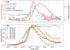 |
Fig. 2. Light curves of the M1.1 flare from 14:30 UT to 15:00 UT on 2023 May 25. Panel (a) shows GOES SXR fluxes at wavelengths of 1−8 Å (solid black line) and its derivative (dotted blue line), and HXI HXR count rates in the energy bands 13−18 keV (solid red line) and 19−30 keV (solid cyan line). Panel (b) shows normalized light curves of CHASE Hα waveband and AIA 94, 131, 171, 193, 211, 304, and 335 Å channels from the brightening region, as shown in the black box in Figure 1b. |
3. Results
3.1. Extrapolations using NLFFF and PFSS models
We applied NLFFF and PFSS (Altschuler & Newkirk 1969; Schatten et al. 1969; Schrijver & De Rosa 2003) extrapolation to the photospheric vector magnetic field data obtained by SDO/HMI to better understand the magnetic field topology and to determine the mechanism of the flare eruption.
We used the minimum-energy approach to resolve a 180° ambiguity in the transverse components of the vector magnetogram. Next, we corrected for projection effects (Guo et al. 2017) using the technique proposed by Gary & Hagyard (1990). We then used the vector magnetic field within a field of view of 400′′ × 320′′ as the boundary. The Message Passing Interface Adaptive Mesh Refinement Versatile Advection Code1 (MPI-AMRVAC; Keppens et al. 2012, 2023; Porth et al. 2014; Xia et al. 2018) was used to extrapolate the potential magnetic field in a Cartesian computation domain resolved by 400 × 320 × 320 uniform grids. Finally, the potential magnetic field was relaxed to an NLFFF state using the magneto-frictional approach (Guo et al. 2016a, 2016b). Different views of the magnetic structure are presented in Figures 3a–3b. The Bz component of the photospheric magnetic field is seen in the background. Sheared arcades are observed beneath a standard fan-spine topology. The arcades coincide with the filament shown in Figure 1.
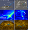 |
Fig. 3. Magnetic structure of the circular ribbon flare. Panels (a)–(b) show nonlinear force-free field (NLFFF) extrapolation in the Cartesian coordinates in two perspectives. Panels (c)–(d) show the distribution of the squashing degree log10Q in the black dashed boxes in panels a–b, respectively. Panel (d) displays a slice at a height of about 11 Mm from the bottom. Panels (e)–(f) show NLFFF extrapolation in spherical coordinates viewed in two perspectives. And the view shown in panel f corresponds to that observed by AIA. |
To better represent the magnetic topology of this structure, we calculated the squashing factor Q with the K-QSL code developed by K. E. Yang2, following the method proposed by Scott et al. (2017) and Tassev & Savcheva (2017). In Figures 3a–3b, the black dashed boxes designate the regions selected for the Q computation. The resulting Q maps are shown in Figures 3c–3d. The squashing factor Q provides useful information on the magnetic field connectivity gradient. The inner and outer spines, the fan structure, the sheared arcade, and a null point are clearly observed in Figure 3c. The null point is located approximately 14 Mm above the negative magnetic polarity. Additionally, we computed the PFSS model using a full-disk synoptic magnetogram and obtained the spherical NLFFF model via magneto-frictional relaxation (Guo et al. 2016a,b). This approach provides a larger field of view and reveals the outer spine in Figures 3e–3f. We projected the field lines onto an SDO/AIA 171 Å image, showing that the position of the remote brightening is in good agreement with the outer-spine footpoint.
Based on the above analysis, we speculate on the evolution process of this flare. The filament rises and undergoes magnetic reconnection at the null point, transferring magnetic twist and cool plasma to the outer spine, ultimately triggering a rotating jet. This dynamic scenario is strongly supported by observational studies (Sterling et al. 2015) and numerical simulations of rotating jet excitation (Fang et al. 2014; Doyle et al. 2019). Simultaneously, large amounts of energy are released during magnetic reconnection at the null point, accelerating energetic particles that follow the fan field lines down to the chromosphere, forming the circular flare ribbon, and along the outer spine lines, forming the remote flare ribbon.
3.2. Analysis of LOS and POS velocities from CHASE
We utilized the full-disk spectral data from the CHASE Hα waveband to derive the LOS and POS velocities. The LOS velocities of the flare ribbon and the cool component of the jet at 14:45:55 UT are displayed in Figure 4a. We derived Doppler velocities using different methods depending on the regions. In the quiet region, where the Hα profile is in pure absorption, the Doppler velocity was determined from the shift of the bisector of the original profile at the 80% level of the nearby continuum. For the flare ribbons, where the line exhibits more or less emissions, we used the net profile (the flare profile with the pre-flare profile at the same position at 13:33 UT subtracted). The velocity was obtained from the shift of the bisector of the net profile at the 20% level of the maximum intensity of the net profile. In the jet regions, the line exhibits a distinct absorption feature in either the blue or the red wing caused by the jet. We therefore determine the velocity of the cool component of the jet according to the position of the local minimum in the wings of the net profile.
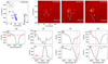 |
Fig. 4. Line-of-sight (LOS) and plane-of-sky (POS) velocities of the flare and the cool component of the jet. Panel (a) shows the Doppler velocity diagram at 14:45:55 UT. Panels (b)–(d) show the temporal evolution of the POS velocity determined by FLCT. Panels (e)–(h) show Hα spectra observed by CHASE in the quiet region (Rq, the average spectral line of the black box in panel a), flare region (Rf), redshift (Rr), and blueshift (Rb) regions of the jet. Panels (i)–(k) show the net line profiles in Rf, Rr, and Rb. The dashed red lines indicate the 80% intensity of Rq, 20% intensity of the emission line of Rf, and the wavelengths corresponding to the intensity minimum of the red wing in Rr and the blue wing in Rb, respectively. |
The background region (Rq), exhibiting no Doppler shift, is marked by the black rectangle in Figure 4a. We computed the mean line profile within this region and used it as the background profile for the jet region. Using the 80%-intensity level bisector approach (see Zhao et al. 2022), the line-core λ0 of Rq was determined, as shown in Figure 4e. The net line profile of the flare ribbon (Rf), obtained by subtracting the pre-flare profile, is an emission line, shown in Figure 4i. The line-core λi was obtained using the 20%-intensity bisector method on the net line profile, and the Doppler velocity was calculated as  . The jet areas (Rr and Rb) exhibit red and blue shifts, with absorption in the red and blue wings of the line profiles, shown in Figures 4g and 4h, respectively. To calculate the Doppler velocity, we used the wavelength λi, which is determined by the minimum intensity shown in Figures 4j and 4k.
To determine the POS velocity field, we employed the Fourier Local Correlation Tracking (FLCT; Welsch et al. 2004, 2007) technique. We traced the evolution of ejected material using the blue-wing enhanced images (Figures 1q–1t), and the POS velocity at three moments is shown in Figures 4b–4d. Whether the POS velocity derived from FLCT truly represents the bulk flow velocity must be examined. First, the energy released by magnetic reconnection may propagate along the outer spine via thermal conduction, heating the jet material and causing it to become unresponsive in the CHASE Hα blue-wing monochromatic image. However, the observed jet front moves forward, while the jet footpoint does not, as seen in Figures 4b–4d. The jet footpoint in the blue wing monochromatic image would initially lose response as thermal conduction travels along the outer spine because it should be heated up from the footpoint first. However, because material is always present at the jet footpoint, we can rule out the influence of thermal conduction. Secondly, the POS velocity could represent the phase velocity of a wave. Comparison of the LOS and POS velocities in Figure 4 shows that the POS velocity is not significantly higher than the LOS velocity. To estimate the Alfvén speed, we calculated the average magnetic field intensity of 24 G in the magnetic flux tube shown in Figure 5a and a mass density of (1.1 − 1.5)×10−10 kg m−3 derived from the emission measure (EM; Su et al. 2018). We then derived the Alfvén speed as  , yielding vA = 175 − 204 km s−1. The vector sum of the LOS and POS velocities at the seven points in Figure 5 range from 50 to 150 km s−1. Therefore, the POS velocity is less likely to represent the phase velocity of an Alfvén wave or a fast-mode magnetoacoustic wave, since it is smaller than the Alfvén velocity. However, due to limitations of the DEM inversion technique, the calculated density reflects only the properties of the hotter component of the jet. If the colder component, which likely has a higher density, is considered, the Alfvén speed should be lower. Therefore, based on our current results, we cannot entirely rule out this scenario. The slow mode magnetoacoustic velocity is equal to the speed of sound along the magnetic field line. Using
  , the speed of sound cs was estimated to be 15 km s−1, assuming that the jet material temperature corresponds to the standard Hα jet value of 104 K (Yokoyama & Shibata 1995). The FLCT analysis focused on tracking POS velocities in CHASE-detected cool plasma, which is sensitive only to low-temperature emissions. This detection constraint naturally limits our study to cold surge material, excluding the surrounding hot plasma. Therefore, the slow-mode magnetoacoustic wave velocity is inconsistent with the vector sum of LOS and POS velocities, which ranged from 50 to 150 km s−1. Furthermore, since CHASE exhibits no response to high-temperature plasma, and the materials detected in CHASE blue-wing images are exclusively localized within jet structures while being completely absent in flare ribbons, we conclude that these features cannot be attributed to chromosphere evaporation, but are more likely associated with jet material. Finally, based on the dashed blue line y = x in Figure 5c, the inclination angle of the velocity is almost equal to that of the magnetic field. This suggests that the velocity is more likely to be the velocity of the cool component of jet bulk flow.
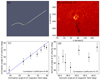 |
Fig. 5. Comparison of the angles between the magnetic field and velocity field along a magnetic field line. Panels (a) shows a field line from Figure 3b (white line), and seven green dots selected along it. Panel (b) shows a CHASE Hα blue-wing enhanced image at 14:45:55 UT. The green points are the projection of the points in panel a, while the orange points indicate the corresponding seven points along the jet used to calculate the velocity. Panels (c)–(d) show the inclination angle (θ) and azimuth angle (ϕ) of the magnetic field and velocity field at the selected points. The blue dashed line shows y = x, indicating that the inclination angle of the velocity equals that of the magnetic field. |
Assuming that the POS velocity corresponds to the jet bulk flow velocity, the actual motion can be derived from the combined POS and LOS velocity measurements. Prior to jet formation, during the ascending phase of the bottom filament, Figure 4b shows the filament moving outward at a moderate velocity at 14:40:01 UT. It then progressively accelerated, reaching a speed of ∼122 km s−1 for the cool component of the jet around 14:45:55 UT, as shown in Figure 4d. The highest jet ejection velocity, combined with the LOS speed of 83 km s−1, is approximately 148 km s−1. The ejection is directed toward the southwest, while some material in the center is moving toward the southeast. This is consistent with the observation that the jet turns counterclockwise toward the southeast during the early phase.
In the supplementary animation for Figure 1, transverse wave-like motions are observed at the jet spire in the hotter passbands. Furthermore, the POS velocities displayed in Figure 4 indicate that the POS motion on the eastern side of the jet spire in Hα likely follows this transverse motion, exemplified by the plasma moving southeastward in Figure 4c. Since the eastern region exhibits the most prominent motion in Hα, our subsequent analysis primarily focuses on this area in Section 3.3.
3.3. Angle of velocity and magnetic field
Here, we analyze angular correlations between the magnetic field and the velocity field of the cool component of the jet. We selected the velocity at 14:45:55 UT to compare with the magnetic field. This period was selected because the FLCT method requires two images: one at the present moment and at the subsequent moment. Thus, we chose the time when the jet is most clearly visible. We tested different times and found that this choice does not influence the final conclusion. We selected seven points along a fan-spine field line (the white line in Figure 3b) and seven points along the jet in the CHASE image, with the same plane projection distance between each point. The seven points (green dots) along the magnetic field line are shown in Figure 5a, whereas the seven points (orange dots) along the jet axis are shown in Figure 5b. The green points from Figure 5a are projected onto the blue-wing enhanced CHASE image in Figure 5b.
We selected only the points near the footpoint of the jet, not the points at the end of the jet. Near the footpoint, the observed jet coincides with the magnetic field line; farther from the footpoint, the observed jet has a certain angle difference with the magnetic field line. This difference is mainly due to the limitation of extrapolation. The magnetic field used as the bottom boundary has a limited field of view and therefore cannot include all information, such as the remote footpoint of the outer spine. The extrapolated magnetic field lines are not completely consistent with the observed direction. This issue is also mentioned by Petrova et al. (2024). The extrapolated magnetic field lines near the footpoint match the observed jet, indicating that comparison with observations is reliable.
We constructed a coordinate system, which is shown in the lower right corner of Figure 5b, with the z axis parallel to the line of sight to compare their angles. Figures 5c and 5d illustrate the inclination angle θ, which is the angle of the velocity/magnetic vector measured from the z axis, and the azimuth angle ϕ, which is the angle of the projected velocity or magnetic vector on the xy plane measured counterclockwise from the x axis.
Figures 5c and 5d show a strong correlation between the inclination and azimuth angle of the velocity and the magnetic field, with correlation coefficients of 0.99 and 0.70, respectively. The dashed blue line in Figure 5c represents y = x, indicating that the inclination angles of the magnetic field and the velocity field are identical. Many data points fall on the y = x line, indicating that the cool bulk flow of the jet probably moves along the outer spine of the magnetic field structure.
3.4. Chromosphere condensation
To investigate the physical mechanism of chromosphere condensation, we fit the energy spectrum of HXI during the HXR peak time 14:43:00−14:44:00 UT, shown in Figure 6. The background was selected from the orbital data 48 hours prior to the spectrum time. We tested both a single thermal model and a double thermal model for fitting, and we find that the single thermal model does not provide a good fit above 23 keV, while the highest temperature in the double thermal model must reach 80 MK, which is almost impossible for M-class flares (Caspi et al. 2014). Therefore, we fit the spectrum in the range of 11−28 keV using a combination of an isothermal component (vth) and a thick-target model (thick2) using the OSPEX spectral analysis package3.
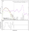 |
Fig. 6. Energy spectrum analysis from HXI. The upper panel shows the HXI hard X-ray spectrum during 14:43:00 UT–14:44:00 UT (black line) after removing the background, with the background energy spectrum shown in purple. The fitted thermal (vth), nonthermal (thick2) components, and their sum (vth+thick2) are indicated by green, yellow, and red lines, respectively. The lower panel shows the normalized residuals. |
Figure 6a shows the fitting results: the black line represents the original energy spectrum, the red line represents the combination of vth and thick2, and Figure 6b shows the χ2 residual. The low-energy cutoff energy Ec = 15.1 keV and the spectral index δ = 10.1. It should be noted that due to the weak response of this M1.1 flare on HXI, fitting the energy spectrum was challenging. Although combining thermal and thick-target model provided a better fit than other models, the uncertainty of each parameter is very large; therefore, these parameters are only provided as a reference and should be used for further analysis with caution.
Assuming that the 13−18 keV band originated mainly from thermal emission and 19−30 keV from nonthermal emission, we located their sources by projecting the hard X-ray sources onto an AIA 94 Å image at 14:43:01 UT separately, as shown in Figures 7a and 7c. The contour levels were set at 90%, 70%, and 50% of the maximum intensity.
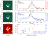 |
Fig. 7. Comparison of HXI flux and CHASE Doppler velocity. Panel (a) shows an AIA 94 Å map during the solar flare, with HXR 13−18 keV emissions at 90%, 70%, and 50% levels indicated by red contours. Panel (b) shows the HXI 13−18 keV flux (red) and CHASE Hα Doppler velocity (black) for the region of the HXR 13−18 keV emission source (red rectangle in panel e), with gray dotted lines marking their peak times. Panels (c)–(d) are similar to panels a–b, but corresponding to the HXR 19−30 keV flux (blue) and Doppler velocity (black) of its source (blue rectangle in panel e). Panel (e) shows the CHASE Hα line-core image at 14:43:33 UT, with the Doppler velocity calculation areas from panels b and d indicated by the red and blue boxes, respectively. Panel (f) shows the scatterplots of Doppler velocities versus the HXR 13−18 keV (red) and 19−30 keV (blue) fluxes, with the Pearson correlation coefficients labeled. |
To investigate the mechanism of chromosphere condensation, we computed the Doppler velocity in relation to the HXR flux. We determined the temporal evolution of the mean Doppler velocity in a small area corresponding to the thermal and nonthermal sources observed by CHASE (marked by the red and blue rectangles in Figure 7e). Figure 7b shows the mean Doppler velocity (black) of the thermal source (red rectangle in panel e) and HXI flux at 13−18 keV (red). Figure 7d displays the HXI flux at 19−30 keV (blue) and the mean Doppler velocity (black) of the nonthermal source (blue rectangle in panel e).
Figure 7f displays the flux-velocity diagram for thermal (red) and nonthermal (blue) regions along with their corresponding Pearson correlation coefficients (0.85 and 0.80). We applied a cross-correlation approach to determine the time offset between the HXI flux and the Doppler velocity, interpolated to the HXI time cadence, because the peak time (dotted gray line) of the CHASE Hα Doppler velocity of the thermal source and the HXI 13−18 keV flux are not strictly aligned in Figure 7b. We find that the Doppler velocity peaked around 58 seconds after the HXI flux peak. Applying the same technique to the two curves in Figure 7d (HXI 19−30 keV flux and Doppler velocity of the nonthermal source), we find that their peak times (gray dotted line) coincide. The thermal and nonthermal particles accelerated by magnetic reconnection first enter the chromosphere along the magnetic field lines and simultaneously produce HXR emission during the chromosphere condensation phase. We deduce that the Doppler velocity and HXR flux should peak simultaneously, based on the physical image above. Consequently, we conclude that nonthermal electrons are more likely to be the primary cause of chromosphere condensation.
The Hα line exhibits redshift and the maximum velocity is approximately 20 km s−1, which is compatible with explosive evaporation. The characteristics of explosive evaporation include blueshift with high speed in the hot lines, redshift with low speed in the cool lines, and an input energy flux exceeding a critical value (1010 erg s−1 cm−2). Nevertheless, due to the large fitting error in the energy spectrum, we were unable to calculate the input energy flux using the fitting parameters. We could not obtain additional information from the high-temperature spectral lines to corroborate this event because neither the EUV Imaging Spectrometer (EIS; Culhane et al. 2007) aboard Hinode nor the Interface Region Imaging Spectrograph (IRIS; De Pontieu et al. 2014) has observed it. Therefore, we do not further confirm the presence of explosive evaporation in this event.
To illustrate the structure of the circular ribbon flare and further investigate the evolution of the thermal and nonthermal HXR sources, we show a composite AIA image of 94, 131, and 335 Å channels in Figure 8a. We mark the circular ribbon (RC), the inner-spine ribbon (RI), the hot flare loop, and the filament in the erupting process that later forms the jet. We made slices at thermal and nonthermal HXR sources, respectively, and show the distance-time diagrams in Figures 8b and 8c. Figure 8b shows that the area around the thermal HXR source steadily warms up before beginning to cool at approximately 14:45 UT. This timing is well in line with the two peak times in Figure 7b.
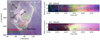 |
Fig. 8. Panel (a) shows a tricolor AIA image with channels in 94 Å (red), 131 Å (green), and 335 Å (blue) at 14:41 UT. The filament, flare loop, circular ribbon (RC), and inner-spine ribbon (RI) are indicated by black arrows. Panels (b)–(c) show distance–time diagrams constructed from slice1 and slice2 in panel a. The changing colors illustrate a heating and cooling process. The borders between dominated AIA passbands are indicated by white dashed lines. |
Figure 8c shows that there is also a response in the hotter waveband 131 Å at the nonthermal emission source. This is consistent with the expectation that the nonthermal component is dominant at 19−30 keV, while the thermal component is still present with less influence. Comparing Figures 8b and 8c, heating occurs at both sources nearly simultaneously, reaching maximum temperature at the same moment, although the temperature at the nonthermal source is lower than that at the thermal source. In other words, at the nonthermal source, the CHASE Doppler velocity and the HXI flux peaked simultaneously, with the temperature peaking a few minutes later. Therefore, we speculate that the nonthermal particles accelerated by magnetic reconnection are the dominant components throughout the process. The nonthermal particles first reach the chromosphere and cause chromosphere condensation. At this time, both the CHASE Doppler velocity and the HXI flux at the nonthermal source simultaneously reach their maxima. The flare ribbon is then heated via heat conduction, causing the temperature of both sources to peak simultaneously.
3.5. Observed jet motions: material flow or wave motion?
This section focuses on the coexistence of material flow and wave-like phenomena within the jet. As shown in Figure 4 and discussed in Section 3.2, the jet exhibits significant field-aligned flows. Furthermore, the accompanying animation to Figure 1 clearly reveals pronounced rotational motions. To further illustrate this rotation, Figure 9 presents the temporal evolution of the SDO/AIA 94 Å emission within slices perpendicular to the jet axis (indicated by the white lines in Figure 1d). The temporal evolution within these two slits reveals periodic motions of the jet material, primarily manifesting as diagonal displacements from the upper left to the lower right. This observed periodic transverse motion deserves further discussion. Fundamentally, this pattern represents transverse material flow, potentially arising from the unidirectional rotation of the jet, as demonstrated by Liu et al. (2009, 2014), where such rotation produces similar periodic transverse displacements.
Alternatively, pulsed Alfvén waves propagating along the jet could also contribute to this signature. Quantifying the motion by tracing the clearest trajectory in each slit in Figure 9 shows transverse velocities of 198.6 km s−1 to 201.8 km s−1, consistent with the Alfvén speed (vA = 175−204 km s−1) estimated in Section 3.2. Pariat et al. (2009), Petrova et al. (2024), and Yang et al. (2025) demonstrate through both observations and simulations that rotating jets may generate pulsed Alfvén waves.
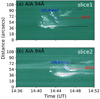 |
Fig. 9. Distance-time diagrams of the slices indicated in Figure 1d, which are perpendicular to the jet axis. |
Furthermore, Alfvén wave oscillations can occur within rotating structures, as noted by Kohutova et al. (2020). However, such oscillations typically require periodic rotation rather than steady unidirectional motion and exhibit small amplitudes. Crucially, Figure 9 shows no evidence of bidirectional rotational motion, and the dominant high-speed field-aligned flow component of the jet would likely mask any superimposed weak oscillatory Alfvénic signal, rendering it undetectable within our current observational constraints.
4. Conclusion and discussion
We have presented a detailed analysis of an M1.1 circular ribbon flare with a rotating jet that occurred on 2023 May 25, based on observations from SDO/AIA, SDO/HMI, ASO-S/HXI, and CHASE. The main conclusions are summarized as follows:
-
(1)
Using magnetic field extrapolation, we reconstructed the 3D magnetic structure of the circular ribbon flare and jet. The fan structure, inner and outer spines, null point, and sheared arcades (corresponding to the filament) that might form the jet are all clearly visible. We hypothesize that the filament at the base lifts upward and undergoes reconnection at the null point, transferring both cool and hot plasma along the outer spine to ultimately form the jet. Simultaneously, magnetic reconnection at the null point produces a large number of energetic particles and heats the lower atmosphere along the fan surface, creating a brightening circular ribbon. These observations are consistent with the widely acknowledged jet model (Canfield et al. 1996; Moore et al. 2010; Sterling et al. 2015) and the circular ribbon flare mechanism (Masson et al. 2009; Sun et al. 2013).
-
(2)
We calculated the LOS and POS velocities using CHASE data and selected a magnetic flux tube from NLFFF extrapolation to compare the angles of the magnetic field on the tube with the velocity field. We find that there is a strong positive linear correlation between their inclination and azimuth angles. This finding suggests that the cool material of the jet moves along the outer spine.
-
(3)
Analysis of the Doppler velocity map reveals chromosphere condensation in the flare ribbon. The process of chromosphere condensation is further examined using ASO-S/HXI observations. Nonthermal particles are essential in chromosphere condensation, as evidenced by the strong association between the temporal evolution of flare ribbon Doppler velocity, nonthermal source HXR flux, and their corresponding peak times.
-
(4)
In addition to field-aligned flows, we analyzed AIA transverse slices to investigate the possible presence of Alfvén waves within the jet. The observed signatures may indicate either propagating Alfvén waves or persistent material flows along the jet, or a combination of both. The highly twisted jet flux rope that reconnects with an untwisted open field line may be the source of this wave (Archontis et al. 2013). However, based on the current data and analysis, we cannot definitively distinguish between these possibilities.
Our comparison of the magnetic field and the velocity field of cool component of the jet derived from CHASE observations provides a clear picture of the magnetic freezing effect. To reconstruct the velocity field of a prominence and a filament, Qiu et al. (2024) used CHASE data to compute the POS velocity via FLCT and the combination of fitting of a single-cloud and double-cloud model to obtain the LOS velocity. Similarly, we also used CHASE observation to reconstruct the velocity field of the jet.
It is worth noting that Tian et al. (2015) report a time delay of 0.5−2.0 minutes between Fe XXI Doppler velocity and the SXR derivative. According to Li et al. (2015), Doppler velocities acquired at various IRIS slit locations exhibit distinct peak periods. In CHASE observations, the use of raster scanning mode (RSM), may explain the delay between the Doppler velocity and HXR flux of the thermal HXR source. Therefore, the possibility of chromosphere condensation as a result of thermal conduction cannot be completely ruled out.
Liu et al. (2009) observed a rotating jet using the Solar Optical Telescope (SOT; Tsuneta et al. 2008) aboard Hinode (Kosugi et al. 2007). In the ascending phase, the jet oscillates transversely, while in the descending phase, it descends straight down. They proposed that the magnetic flux rope releases magnetic helicity and creates a torsional Alfvén wave when it reconnects with the open field lines after ejection. Shen et al. (2011) used the Solar Magnetic Activity Research Telescope (SMART; Ueno et al. 2004) and SDO/AIA to study an untwisting polar jet. They suggested that the free energy stored in the non-potential magnetic field can be released through untwisting of the flux rope and that this energy was sufficient to provide energy for the ejection. Their findings support the theory that a small twisted bipolar closed field stores magnetic energy, which can be released through magnetic reconnection between the bipolar and its surrounding open field. A 3D Cartesian MHD numerical simulation of torsional Alfvén waved produced by the magnetic reconnection of a twisted magnetic flux rope with open field lines was conducted by Archontis et al. (2013) and Wyper et al. (2018). The Alfvén waves potentially present within this jet may be explained by the studies mentioned above, namely that they are generated by magnetic reconnection of the twisted flux rope with open field lines.
Data availability
Movie associated to Fig. 1 is available at https://www.aanda.org
Acknowledgments
We appreciate the NASA/SDO team providing the AIA and HMI data. The CHASE launch is supported by China National Space. ASO-S mission is supported by the Strategic Priority Research Program on Space Science, the Chinese Academy of Sciences. L.H., Y.G., C.Z., and M.D.D. were supported by the National Key R&D Program of China (2022YFF0503004, 2021YFA1600504, and 2020YFC2201201) and NSFC (12333009 and 12127901). Y.S. is supported by the National Key R&D Program of China 2022YFF0503002, the Strategic Priority Research Program of the Chinese Academy of Sciences (Grant No. XDB0560000), and the NSFC 12333010. Z.T.L. is supported by the Prominent Postdoctoral Project of Jiangsu Province (2023ZB304).
References
- Altschuler, M. D., & Newkirk, G. 1969, Sol. Phys., 9, 131 [NASA ADS] [CrossRef] [Google Scholar]
- Archontis, V., Hood, A. W., & Tsinganos, K. 2013, ApJ, 778, 42 [Google Scholar]
- Ashfield, W. H., & Longcope, D. W. 2021, ApJ, 912, 25 [Google Scholar]
- Battaglia, M., Kleint, L., Krucker, S., & Graham, D. 2015, ApJ, 813, 113 [Google Scholar]
- Brosius, J. W. 2009, ApJ, 701, 1209 [Google Scholar]
- Brueckner, G. E., & Bartoe, J. D. F. 1983, ApJ, 272, 329 [Google Scholar]
- Canfield, R. C., Reardon, K. P., Leka, K. D., et al. 1996, ApJ, 464, 1016 [NASA ADS] [CrossRef] [Google Scholar]
- Carmichael, H. 1964, NASA Spec. Publ., 50, 451 [NASA ADS] [Google Scholar]
- Caspi, A., Krucker, S., & Lin, R. P. 2014, ApJ, 781, 43 [NASA ADS] [CrossRef] [Google Scholar]
- Chandra, R., Mandrini, C. H., Schmieder, B., et al. 2017, A&A, 598, A41 [NASA ADS] [CrossRef] [EDP Sciences] [Google Scholar]
- Chen, B., Li, H., Song, K.-F., et al. 2019, RAA, 19, 159 [Google Scholar]
- Chen, D.-Y., Hu, Y.-M., Ma, T., et al. 2021, RAA, 21, 136 [Google Scholar]
- Cheng, X., Guo, Y., & Ding, M. 2017, Sci. China Earth Sci., 60, 1383 [Google Scholar]
- Culhane, J. L., Harra, L. K., James, A. M., et al. 2007, Sol. Phys., 243, 19 [Google Scholar]
- Czaykowska, A., De Pontieu, B., Alexander, D., & Rank, G. 1999, ApJ, 521, L75 [Google Scholar]
- De Pontieu, B., Carlsson, M., Rouppe van der Voort, L. H. M., et al. 2012, ApJ, 752, L12 [Google Scholar]
- De Pontieu, B., Title, A. M., Lemen, J. R., et al. 2014, Sol. Phys., 289, 2733 [Google Scholar]
- del Zanna, G., Berlicki, A., Schmieder, B., & Mason, H. E. 2006, Sol. Phys., 234, 95 [Google Scholar]
- Doschek, G. A., Warren, H. P., & Young, P. R. 2013, ApJ, 767, 55 [NASA ADS] [CrossRef] [Google Scholar]
- Doyle, L., Wyper, P. F., Scullion, E., et al. 2019, ApJ, 887, 246 [Google Scholar]
- Falewicz, R., Rudawy, P., & Siarkowski, M. 2009, A&A, 508, 971 [NASA ADS] [CrossRef] [EDP Sciences] [Google Scholar]
- Fang, F., Fan, Y., & McIntosh, S. W. 2014, ApJ, 789, L19 [NASA ADS] [CrossRef] [Google Scholar]
- Filippov, B., Srivastava, A. K., Dwivedi, B. N., et al. 2015, MNRAS, 451, 1117 [Google Scholar]
- Fisher, G. H., Canfield, R. C., & McClymont, A. N. 1985a, ApJ, 289, 425 [Google Scholar]
- Fisher, G. H., Canfield, R. C., & McClymont, A. N. 1985b, ApJ, 289, 414 [NASA ADS] [CrossRef] [Google Scholar]
- Gan, W., Zhu, C., Deng, Y., et al. 2023, Sol. Phys., 298, 68 [NASA ADS] [CrossRef] [Google Scholar]
- Gary, G. A., & Hagyard, M. J. 1990, Sol. Phys., 126, 21 [Google Scholar]
- Gosling, J. T., Hildner, E., MacQueen, R. M., et al. 1974, J. Geophys. Res., 79, 4581 [Google Scholar]
- Graham, D. R., Cauzzi, G., Zangrilli, L., et al. 2020, ApJ, 895, 6 [Google Scholar]
- Guo, Y., Xia, C., & Keppens, R. 2016a, ApJ, 828, 83 [NASA ADS] [CrossRef] [Google Scholar]
- Guo, Y., Xia, C., Keppens, R., & Valori, G. 2016b, ApJ, 828, 82 [NASA ADS] [CrossRef] [Google Scholar]
- Guo, Y., Cheng, X., & Ding, M. 2017, Sci. China Earth Sci., 60, 1408 [Google Scholar]
- Hao, Q., Yang, K., Cheng, X., et al. 2017, Nat. Commun., 8, 2202 [Google Scholar]
- Hirayama, T. 1974, Sol. Phys., 34, 323 [Google Scholar]
- Jibben, P., & Canfield, R. C. 2004, ApJ, 610, 1129 [NASA ADS] [CrossRef] [Google Scholar]
- Joshi, N. C., Liu, C., Sun, X., et al. 2015, ApJ, 812, 50 [Google Scholar]
- Kaiser, M. L., Kucera, T. A., Davila, J. M., et al. 2008, Space Sci. Rev., 136, 5 [Google Scholar]
- Kamio, S., Kurokawa, H., Brooks, D. H., Kitai, R., & UeNo, S. 2005, ApJ, 625, 1027 [Google Scholar]
- Keppens, R., Meliani, Z., van Marle, A. J., et al. 2012, J. Comput. Phys., 231, 718 [Google Scholar]
- Keppens, R., Popescu Braileanu, B., Zhou, Y., et al. 2023, A&A, 673, A66 [NASA ADS] [CrossRef] [EDP Sciences] [Google Scholar]
- Kohutova, P., Verwichte, E., & Froment, C. 2020, A&A, 633, L6 [NASA ADS] [CrossRef] [EDP Sciences] [Google Scholar]
- Kopp, R. A., & Pneuman, G. W. 1976, Sol. Phys., 50, 85 [Google Scholar]
- Kosugi, T., Matsuzaki, K., Sakao, T., et al. 2007, Sol. Phys., 243, 3 [Google Scholar]
- Kumar, P., Karpen, J. T., Antiochos, S. K., et al. 2018, AGU Fall Meeting Abstracts, 2018, SH13A–03 [Google Scholar]
- Lee, E. J., Archontis, V., & Hood, A. W. 2015, ApJ, 798, L10 [Google Scholar]
- Lee, K.-S., Imada, S., Watanabe, K., Bamba, Y., & Brooks, D. H. 2017, ApJ, 836, 150 [NASA ADS] [CrossRef] [Google Scholar]
- Lemen, J. R., Title, A. M., Akin, D. J., et al. 2012, Sol. Phys., 275, 17 [Google Scholar]
- Li, Y., & Ding, M. D. 2011, ApJ, 727, 98 [NASA ADS] [CrossRef] [Google Scholar]
- Li, D., Ning, Z. J., & Zhang, Q. M. 2015, ApJ, 813, 59 [Google Scholar]
- Li, H., Jiang, Y., Yang, J., et al. 2017, ApJ, 836, 235 [Google Scholar]
- Li, Y., Ding, M. D., Hong, J., Li, H., & Gan, W. Q. 2019a, ApJ, 879, 30 [NASA ADS] [CrossRef] [Google Scholar]
- Li, H., Chen, B., Feng, L., et al. 2019b, RAA, 19, 158 [Google Scholar]
- Li, C., Fang, C., Li, Z., et al. 2022, Sci. China Phys. Mech. Astron., 65, 289602 [NASA ADS] [CrossRef] [Google Scholar]
- Li, D., Li, C., Qiu, Y., et al. 2023, ApJ, 954, 7 [Google Scholar]
- Libbrecht, T., de la Cruz Rodríguez, J., Danilovic, S., Leenaarts, J., & Pazira, H. 2019, A&A, 621, A35 [NASA ADS] [CrossRef] [EDP Sciences] [Google Scholar]
- Liu, W., Berger, T. E., Title, A. M., & Tarbell, T. D. 2009, ApJ, 707, L37 [NASA ADS] [CrossRef] [Google Scholar]
- Liu, J., Wang, Y., Liu, R., et al. 2014, ApJ, 782, 94 [Google Scholar]
- Liu, C., Deng, N., Liu, R., et al. 2015, ApJ, 812, L19 [Google Scholar]
- Lu, L., Li, H., Huang, Y., et al. 2020, Acta Astron. Sin., 61, 38 [Google Scholar]
- Masson, S., Pariat, E., Aulanier, G., & Schrijver, C. J. 2009, ApJ, 700, 559 [Google Scholar]
- Masson, S., Pariat, É., Valori, G., et al. 2017, A&A, 604, A76 [EDP Sciences] [Google Scholar]
- Milligan, R. O., Gallagher, P. T., Mathioudakis, M., & Keenan, F. P. 2006, ApJ, 642, L169 [NASA ADS] [CrossRef] [Google Scholar]
- Moore, R. L., Cirtain, J. W., Sterling, A. C., & Falconer, D. A. 2010, ApJ, 720, 757 [Google Scholar]
- Neupert, W. M. 1968, ApJ, 153, L59 [NASA ADS] [CrossRef] [Google Scholar]
- Pariat, E., Antiochos, S. K., & DeVore, C. R. 2009, ApJ, 691, 61 [Google Scholar]
- Pesnell, W. D., Thompson, B. J., & Chamberlin, P. C. 2012, Sol. Phys., 275, 3 [Google Scholar]
- Petrova, E., Van Doorsselaere, T., Berghmans, D., et al. 2024, A&A, 687, A13 [NASA ADS] [CrossRef] [EDP Sciences] [Google Scholar]
- Porth, O., Xia, C., Hendrix, T., Moschou, S. P., & Keppens, R. 2014, ApJS, 214, 4 [Google Scholar]
- Priest, E. R., Parnell, C. E., & Martin, S. F. 1994, ApJ, 427, 459 [Google Scholar]
- Qiu, Y., Rao, S., Li, C., et al. 2022, Sci. China Phys. Mech. Astron., 65, 289603 [NASA ADS] [CrossRef] [Google Scholar]
- Qiu, Y., Li, C., Guo, Y., et al. 2024, ApJ, 961, L30 [NASA ADS] [CrossRef] [Google Scholar]
- Raftery, C. L., Gallagher, P. T., Milligan, R. O., & Klimchuk, J. A. 2009, A&A, 494, 1127 [NASA ADS] [CrossRef] [EDP Sciences] [Google Scholar]
- Raouafi, N. E., Patsourakos, S., Pariat, E., et al. 2016, Space Sci. Rev., 201, 1 [Google Scholar]
- Reep, J. W., & Russell, A. J. B. 2016, ApJ, 818, L20 [Google Scholar]
- Roy, J. R. 1973, Sol. Phys., 32, 139 [NASA ADS] [CrossRef] [Google Scholar]
- Sadykov, V. M., Kosovichev, A. G., Sharykin, I. N., & Kerr, G. S. 2019, ApJ, 871, 2 [NASA ADS] [CrossRef] [Google Scholar]
- Schatten, K. H., Wilcox, J. M., & Ness, N. F. 1969, Sol. Phys., 6, 442 [Google Scholar]
- Schmieder, B., Guo, Y., Moreno-Insertis, F., et al. 2013, A&A, 559, A1 [NASA ADS] [CrossRef] [EDP Sciences] [Google Scholar]
- Schou, J., Borrero, J. M., Norton, A. A., et al. 2012, Sol. Phys., 275, 327 [Google Scholar]
- Schrijver, C. J., & De Rosa, M. L. 2003, Sol. Phys., 212, 165 [Google Scholar]
- Scott, R. B., Pontin, D. I., & Hornig, G. 2017, ApJ, 848, 117 [NASA ADS] [CrossRef] [Google Scholar]
- Shen, Y. 2021, Proc. Roy. Soc. London Ser. A, 477, 217 [NASA ADS] [Google Scholar]
- Shen, Y., Liu, Y., Su, J., & Ibrahim, A. 2011, ApJ, 735, L43 [NASA ADS] [CrossRef] [Google Scholar]
- Shetye, J., Verwichte, E., Stangalini, M., et al. 2019, ApJ, 881, 83 [Google Scholar]
- Shibata, K., & Magara, T. 2011, Liv. Rev. Sol. Phys., 8, 6 [Google Scholar]
- Shibata, K., & Uchida, Y. 1985, PASJ, 37, 31 [NASA ADS] [Google Scholar]
- Shibata, K., & Uchida, Y. 1986, Sol. Phys., 103, 299 [NASA ADS] [CrossRef] [Google Scholar]
- Shibata, K., Ishido, Y., Acton, L. W., et al. 1992, PASJ, 44, L173 [Google Scholar]
- Shimojo, M., Narukage, N., Kano, R., et al. 2007, PASJ, 59, S745 [Google Scholar]
- Sterling, A. C., Moore, R. L., Falconer, D. A., & Adams, M. 2015, Nature, 523, 437 [NASA ADS] [CrossRef] [Google Scholar]
- Sturrock, P. A. 1968, in Structure and Development of Solar Active Regions, ed. K. O. Kiepenheuer, 35, 471 [NASA ADS] [CrossRef] [Google Scholar]
- Su, Y., Veronig, A. M., Hannah, I. G., et al. 2018, ApJ, 856, L17 [NASA ADS] [CrossRef] [Google Scholar]
- Su, Y., Liu, W., Li, Y.-P., et al. 2019, RAA, 19, 163 [Google Scholar]
- Sun, X., Hoeksema, J. T., Liu, Y., et al. 2013, ApJ, 778, 139 [Google Scholar]
- Tassev, S., & Savcheva, A. 2017, ApJ, 840, 89 [NASA ADS] [CrossRef] [Google Scholar]
- Teriaca, L., Falchi, A., Falciani, R., Cauzzi, G., & Maltagliati, L. 2006, A&A, 455, 1123 [NASA ADS] [CrossRef] [EDP Sciences] [Google Scholar]
- Tian, H., Li, G., Reeves, K. K., et al. 2014, ApJ, 797, L14 [Google Scholar]
- Tian, H., Young, P. R., Reeves, K. K., et al. 2015, ApJ, 811, 139 [NASA ADS] [CrossRef] [Google Scholar]
- Török, T., Aulanier, G., Schmieder, B., Reeves, K. K., & Golub, L. 2009, ApJ, 704, 485 [Google Scholar]
- Tousey, R. 1973, Space Res. Conf., 2, 713 [Google Scholar]
- Tsuneta, S., Ichimoto, K., Katsukawa, Y., et al. 2008, Sol. Phys., 249, 167 [Google Scholar]
- Ueno, S., Nagata, S., Kitai, R., & Kurokawa, H. 2004, ASP Conf. Ser., 325, 319 [Google Scholar]
- Van Damme, H. J., De Moortel, I., Pagano, P., & Johnston, C. D. 2020, A&A, 635, A174 [NASA ADS] [CrossRef] [EDP Sciences] [Google Scholar]
- Van Doorsselaere, T., Nakariakov, V. M., & Verwichte, E. 2008, ApJ, 676, L73 [Google Scholar]
- Velli, M., & Liewer, P. 1999, Space Sci. Rev., 87, 339 [Google Scholar]
- Wang, H., & Liu, C. 2012, ApJ, 760, 101 [Google Scholar]
- Warren, H. P., Reep, J. W., Crump, N. A., & Simões, P. J. A. 2016, ApJ, 829, 35 [Google Scholar]
- Wedemeyer-Böhm, S., Scullion, E., Steiner, O., et al. 2012, Nature, 486, 505 [Google Scholar]
- Welsch, B. T., Fisher, G. H., Abbett, W. P., & Regnier, S. 2004, ApJ, 610, 1148 [NASA ADS] [CrossRef] [Google Scholar]
- Welsch, B. T., Abbett, W. P., De Rosa, M. L., et al. 2007, ApJ, 670, 1434 [NASA ADS] [CrossRef] [Google Scholar]
- Williams, D. R. 2004, ESA Spec. Publ., 547, 513 [Google Scholar]
- Wuelser, J.-P., Canfield, R. C., Acton, L. W., et al. 1994, ApJ, 424, 459 [Google Scholar]
- Wyper, P. F., DeVore, C. R., Karpen, J. T., Antiochos, S. K., & Yeates, A. R. 2018, ApJ, 864, 165 [NASA ADS] [CrossRef] [Google Scholar]
- Xia, C., Teunissen, J., El Mellah, I., Chané, E., & Keppens, R. 2018, ApJS, 234, 30 [Google Scholar]
- Xu, A. A., Yin, S. Y., & Ding, J. P. 1984, Acta Astron. Sin., 25, 119 [Google Scholar]
- Xue, Z., Yan, X., Cheng, X., et al. 2016, Nat. Commun., 7, 11837 [Google Scholar]
- Yan, X. L., Qu, Z. Q., & Kong, D. F. 2012, AJ, 143, 56 [Google Scholar]
- Yang, K., Guo, Y., & Ding, M. D. 2015, ApJ, 806, 171 [Google Scholar]
- Yang, L., He, J., Feng, X., et al. 2025, ApJ, 982, L25 [Google Scholar]
- Yokoyama, T., & Shibata, K. 1995, Nature, 375, 42 [Google Scholar]
- Zhang, Z., Chen, D.-Y., Wu, J., et al. 2019, RAA, 19, 160 [NASA ADS] [Google Scholar]
- Zhao, J., Rajaguru, S. P., & Chen, R. 2022, ApJ, 933, 109 [Google Scholar]
All Figures
|
Fig. 1. Overview of the circular ribbon flare. Panels (a)–(d) show images observed by SDO/AIA 94 Å; panels (e)–(h), images observed by SDO/AIA 171 Å; panels (i)–(l), images observed by SDO/AIA 304 Å; panels (m)–(p), CHASE Hα line core (6562.82 Å) images; panels (q)–(t), CHASE Hα blue-wing (6562.82 Å−1.4 Å) enhanced images; and panels (u)–(x), ASO-S LST/SDI Lyman–α waveband (1216 Å) images. From left to right, each column shows images at nearly the same time. The filament, circular ribbon, jet, outer spine, and remote brightening are indicated by white arrows and rectangles. The two white lines labeled slice1 and slice2 in panel d indicate the positions of the slices shown in Figures 9a and 9b. |
| In the text | |
|
Fig. 2. Light curves of the M1.1 flare from 14:30 UT to 15:00 UT on 2023 May 25. Panel (a) shows GOES SXR fluxes at wavelengths of 1−8 Å (solid black line) and its derivative (dotted blue line), and HXI HXR count rates in the energy bands 13−18 keV (solid red line) and 19−30 keV (solid cyan line). Panel (b) shows normalized light curves of CHASE Hα waveband and AIA 94, 131, 171, 193, 211, 304, and 335 Å channels from the brightening region, as shown in the black box in Figure 1b. |
| In the text | |
|
Fig. 3. Magnetic structure of the circular ribbon flare. Panels (a)–(b) show nonlinear force-free field (NLFFF) extrapolation in the Cartesian coordinates in two perspectives. Panels (c)–(d) show the distribution of the squashing degree log10Q in the black dashed boxes in panels a–b, respectively. Panel (d) displays a slice at a height of about 11 Mm from the bottom. Panels (e)–(f) show NLFFF extrapolation in spherical coordinates viewed in two perspectives. And the view shown in panel f corresponds to that observed by AIA. |
| In the text | |
|
Fig. 4. Line-of-sight (LOS) and plane-of-sky (POS) velocities of the flare and the cool component of the jet. Panel (a) shows the Doppler velocity diagram at 14:45:55 UT. Panels (b)–(d) show the temporal evolution of the POS velocity determined by FLCT. Panels (e)–(h) show Hα spectra observed by CHASE in the quiet region (Rq, the average spectral line of the black box in panel a), flare region (Rf), redshift (Rr), and blueshift (Rb) regions of the jet. Panels (i)–(k) show the net line profiles in Rf, Rr, and Rb. The dashed red lines indicate the 80% intensity of Rq, 20% intensity of the emission line of Rf, and the wavelengths corresponding to the intensity minimum of the red wing in Rr and the blue wing in Rb, respectively. |
| In the text | |
|
Fig. 5. Comparison of the angles between the magnetic field and velocity field along a magnetic field line. Panels (a) shows a field line from Figure 3b (white line), and seven green dots selected along it. Panel (b) shows a CHASE Hα blue-wing enhanced image at 14:45:55 UT. The green points are the projection of the points in panel a, while the orange points indicate the corresponding seven points along the jet used to calculate the velocity. Panels (c)–(d) show the inclination angle (θ) and azimuth angle (ϕ) of the magnetic field and velocity field at the selected points. The blue dashed line shows y = x, indicating that the inclination angle of the velocity equals that of the magnetic field. |
| In the text | |
|
Fig. 6. Energy spectrum analysis from HXI. The upper panel shows the HXI hard X-ray spectrum during 14:43:00 UT–14:44:00 UT (black line) after removing the background, with the background energy spectrum shown in purple. The fitted thermal (vth), nonthermal (thick2) components, and their sum (vth+thick2) are indicated by green, yellow, and red lines, respectively. The lower panel shows the normalized residuals. |
| In the text | |
|
Fig. 7. Comparison of HXI flux and CHASE Doppler velocity. Panel (a) shows an AIA 94 Å map during the solar flare, with HXR 13−18 keV emissions at 90%, 70%, and 50% levels indicated by red contours. Panel (b) shows the HXI 13−18 keV flux (red) and CHASE Hα Doppler velocity (black) for the region of the HXR 13−18 keV emission source (red rectangle in panel e), with gray dotted lines marking their peak times. Panels (c)–(d) are similar to panels a–b, but corresponding to the HXR 19−30 keV flux (blue) and Doppler velocity (black) of its source (blue rectangle in panel e). Panel (e) shows the CHASE Hα line-core image at 14:43:33 UT, with the Doppler velocity calculation areas from panels b and d indicated by the red and blue boxes, respectively. Panel (f) shows the scatterplots of Doppler velocities versus the HXR 13−18 keV (red) and 19−30 keV (blue) fluxes, with the Pearson correlation coefficients labeled. |
| In the text | |
|
Fig. 8. Panel (a) shows a tricolor AIA image with channels in 94 Å (red), 131 Å (green), and 335 Å (blue) at 14:41 UT. The filament, flare loop, circular ribbon (RC), and inner-spine ribbon (RI) are indicated by black arrows. Panels (b)–(c) show distance–time diagrams constructed from slice1 and slice2 in panel a. The changing colors illustrate a heating and cooling process. The borders between dominated AIA passbands are indicated by white dashed lines. |
| In the text | |
|
Fig. 9. Distance-time diagrams of the slices indicated in Figure 1d, which are perpendicular to the jet axis. |
| In the text | |
Current usage metrics show cumulative count of Article Views (full-text article views including HTML views, PDF and ePub downloads, according to the available data) and Abstracts Views on Vision4Press platform.
Data correspond to usage on the plateform after 2015. The current usage metrics is available 48-96 hours after online publication and is updated daily on week days.
Initial download of the metrics may take a while.