| Issue |
A&A
Volume 702, October 2025
|
|
|---|---|---|
| Article Number | A260 | |
| Number of page(s) | 17 | |
| Section | Extragalactic astronomy | |
| DOI | https://doi.org/10.1051/0004-6361/202452718 | |
| Published online | 28 October 2025 | |
A theoretical investigation of far-infrared fine structure lines at z > 6 and of the origin of the [O III]88 μm/[C II]158 μm enhancement
1
Institute of Theoretical Astrophysics, University of Oslo, PO Box 1029
Blindern, 0315
Oslo, Norway
2
Lund Observatory, Division of Astrophysics, Department of Physics, Lund University, Box 43
SE-221 00
Lund, Sweden
⋆ Corresponding author: This email address is being protected from spambots. You need JavaScript enabled to view it.
Received:
23
October
2024
Accepted:
17
July
2025
Abstract
The far-infrared (FIR) fine structure lines [C II]158 μm, [O III]88 μm, [N II]122 μm, and [N III]57 μm are excellent tools for probing the physical conditions of the interstellar medium (ISM). The [O III]88 μm/[C II]158 μm and [O III]88 μm/[N II]122 μm luminosity ratios have shown to be promising tracers of the ionisation state and gas-phase metallicity of the ISM. Observations of galaxies at redshift z > 6 show unusually high [O III]88 μm/[C II]158 μm luminosity ratios compared to local sources. The origin of the enhanced ratios has been investigated in the literature with different theoretical modelling approaches. However, no model has to date successfully managed to match the observed emission from both [O III]88 μm and [C II]158 μm, as well as their ratio. For this study we used CLOUDY to model the [C II]158 μm, [O III]88 μm, [N II]122 μm, and [N III]57 μm emission lines of PONOS, a high-resolution (mgas = 883.4 M⊙) cosmological zoom-in simulation of a galaxy at redshift z = 6.5, which is post-processed using KRAMSES-RT. We modify carbon, nitrogen, and oxygen abundances in our CLOUDY models to obtain C/O and N/O abundance ratios respectively lower and higher than solar, more in line with recent high-z observational constraints. We find [O III]88 μm/[C II]158 μm luminosity ratios that are a factor of ∼5 higher compared to models assuming solar abundances. Additionally, we find an overall better agreement of the simulation with high-z observational constraints of the [C II]158 μm-SFR and [O III]88 μm-SFR relations. This shows that a lower C/O abundance ratio is essential to reproduce the enhanced [O III]88 μm/[C II]158 μm luminosity ratios observed at z > 6. By assuming a super-solar N/O ratio, motivated by recent z > 6 JWST observations, our models yield an [O III]88 μm/[N II]122 μm ratio of 1.3, which, according to current theoretical models, would be more appropriate for a galaxy with a lower ionisation parameter than the one we estimated for PONOS. Most current simulations adopt solar abundance patterns that are not adequate for recently observed high-z predictions. Our results showcase the importance of theoretical modelling efforts, coupled with high-resolution zoom-in simulations, and with parallel multi-tracer observations to understand the physical and chemical conditions of the ISM at z > 6.
Key words: methods: numerical / ISM: abundances / ISM: lines and bands / galaxies: evolution / galaxies: high-redshift / galaxies: ISM
© The Authors 2025
 Open Access article, published by EDP Sciences, under the terms of the Creative Commons Attribution License (https://creativecommons.org/licenses/by/4.0), which permits unrestricted use, distribution, and reproduction in any medium, provided the original work is properly cited.
This article is published in open access under the Subscribe to Open model. This email address is being protected from spambots. You need JavaScript enabled to view it. to support open access publication.
1. Introduction
With the formation of the first stars and galaxies, the intergalactic medium (IGM) transitioned from neutral to ionised during the Epoch of Reionisation (EoR) (Robertson 2022), which has been empirically shown to have ended at z ≈ 6 (Fan et al. 2002; Stark et al. 2010; Robertson et al. 2015). At z > 6, galaxies are less dynamically settled as they experience cold mode accretion (Dekel et al. 2009) and frequent interactions (Lacey & Cole 1993; Hopkins et al. 2010; Somerville & Davé 2015; Posses et al. 2025). The gas-phase metallicity in the interstellar medium (ISM) is expected to be low at z > 6, due to core-collapse supernovae (cc-SNe) being the main enrichment mechanism on short timescales (Maiolino & Mannucci 2019). By pushing the frontiers of high-z observations, the James Webb Space Telescope (JWST) has spectroscopically confirmed luminous galaxies out to z ∼ 14 (Carniani et al. 2024; Schouws et al. 2025a; Naidu et al. 2025), enabling us to study galaxies at the beginning of the EoR. Understanding the properties of the ISM at z > 6 is crucial to gaining insight into the early stages of galaxy formation and evolution.
At z > 6, commonly employed ISM gas tracers producing rest-frame lines in the ultraviolet and optical bands are redshifted to wavelengths inaccessible from Earth. However, far-infrared (FIR) emission lines from atomic and ionised gas are redshifted into the sub-millimetre (sub-mm) atmospheric windows. They are thus observable with ground-based facilities placed on high-altitude sites, such as the Atacama Large Millimeter/submillimeter Array (ALMA) and, in the future, the Atacama Large Aperture Submillimeter Telescope (AtLAST)1. The advantage of FIR lines is that they are bright tracers of the cold and warm ISM where star formation is occurring (De Looze et al. 2014; Herrera-Camus et al. 2015), in addition to being less affected by dust-extinction compared to optical lines (Brauher et al. 2008; Ferkinhoff et al. 2010). Most high-z sub-mm observations target the emission lines from singly ionised carbon (C+), [C II]158 μm (hereafter [C II] ), and from doubly ionised oxygen (O++), [O III]88 μm (hereafter [O III] ). [C II] is one of the main coolants of the ISM (Tielens & Hollenbach 1985; Wolfire et al. 2022), making up 0.1–1% of the total FIR emission of a star-forming galaxy (Stacey et al. 1991). Due to its ionisation potential (11.26 eV) lower than hydrogen (13.6 eV) (Cormier et al. 2015), C+ can reside co-spatially with neutral atomic, molecular, and ionised gas (Olsen et al. 2015, 2017; Lagache et al. 2018; Leung et al. 2020). Most of the [C II] emission is believed to originate from photodissociation regions (PDRs) (Stacey et al. 2010). [O III] is a tracer of the warm-hot ionised gas (T ∼ 104–5 × 10⁵ K), and of H II regions (Cormier et al. 2015). Due to the high ionisation potential of O++ (35.1 eV), [O III] probes radiation from hot young stars and is thus a good extinction-free tracer of star formation (Ferkinhoff et al. 2010). The [C II] and [O III] emission lines have been investigated in z > 6 observations (e.g. Kanekar et al. 2013; Ouchi et al. 2013; Capak et al. 2015; Maiolino et al. 2015; Inoue et al. 2016; Laporte et al. 2017; Hashimoto et al. 2018; Tamura et al. 2019; Schaerer et al. 2020; Vanderhoof et al. 2022; Posses et al. 2025; Schouws et al. 2025a,b); however, the number of galaxies where both [C II] and [O III] are detected is still limited (e.g. Inoue et al. 2016; Carniani et al. 2017; Hashimoto et al. 2019; Harikane et al. 2020; Witstok et al. 2022; Fujimoto et al. 2024; Ren et al. 2023; Algera et al. 2024; Kumari et al. 2024; Schouws et al. 2025b). Both [C II] and [O III] have been empirically shown to correlate with the star formation rate (SFR) of galaxies (De Looze et al. 2014; Herrera-Camus et al. 2015). Additionally, since the [O III] and [C II] emission lines trace different gas phases, we can use their luminosity ratios to study the ionisation state of the ISM (Harikane et al. 2020). In local galaxies, the [O III]/[C II] luminosity ratio is observed to be ≲1, while for galaxies at z > 6 with comparable SFR, this value is significantly higher with [O III]/[C II] values ∼1 − 20 (Harikane et al. 2020). The origin of the enhanced high-z[O III]/[C II] ratios is still debated. Several contributing factors have been proposed, such as lower PDR covering fractions, higher ionisation parameters, and lower gas-phase metallicities (Harikane et al. 2020; Arata et al. 2020; Lupi et al. 2020; Vallini et al. 2021; Katz et al. 2022).
The [N II]122 μm line (hereafter [N II] ) from singly ionised nitrogen N+, and [N III]57 μm (hereafter [N III] ), from doubly ionised nitrogen N++, are both tracers of ionised gas (Cormier et al. 2015), with ionisation potentials of 14.53 eV and 29.6 eV respectively. Together with [C II] and [O III], [N II] and [N III] can be used to study the ionisation parameter and gas-phase metallicity of the ISM (Nagao et al. 2011; Pereira-Santaella et al. 2017; Rigopoulou et al. 2018; Schimek et al. 2024b). The current number of observational constraints for the [N II] and [N III] lines is limited. The [N II] line has only been observed in a few non-quasar galaxies at z > 6, with the detection of [N II]122 μm(Killi et al. 2023) and of [N II]205 μm (Tadaki et al. 2022; Kolupuri et al. 2025; Fudamoto et al. 2025), while the [N III] line has yet to be detected at such high redshifts.
Theoretical efforts can help us place the properties of the high-z ISM into the broader context of galaxy formation and evolution. Recent studies include semi-analytical models (e.g. Lagache et al. 2018; Popping et al. 2019), cosmological zoom-in simulations focusing on small galaxy samples (≲10 − 30 galaxies; e.g. Vallini et al. 2015, 2018, 2021; Katz et al. 2019; Olsen et al. 2017; Pallottini et al. 2019; Lupi et al. 2020; Arata et al. 2020), and simulations with large samples of galaxies (Katz et al. 2022; Pallottini et al. 2022; Ramos Padilla et al. 2023; Nakazato et al. 2025). Despite the variety of theoretical modelling approaches, no model has been successful at simultaneously reproducing the high [O III]/[C II] ratios observed at z > 6 and the [C II] and [O III] luminosity values consistent with the high-z [C II]-SFR and [O III]-SFR empirical relations. In contrast to [O III] and [C II], the [N II] and [N III] lines at z ≳ 6 have only been investigated in a few theoretical studies (Ramos Padilla et al. 2023; Schimek et al. 2024b), resulting in the [N II]-SFR and [N III]-SFR relations being poorly constrained at high z.
Most current theoretical models assume solar abundance patterns when accounting for the ISM chemistry, as it is computationally expensive to trace the element abundances directly for each cell (Olsen et al. 2017; Vallini et al. 2018; Pallottini et al. 2019, 2022; Ramos Padilla et al. 2023). However, recent observational constraints from JWST have revealed that the chemistry at z > 6 could be vastly different from the local ISM, with observations of sub-solar C/O abundance ratios and super-solar N/O abundance ratios (Jones et al. 2023; Isobe et al. 2023; Cameron et al. 2023), making the assumption of solar values unrealistic when modelling the high-z ISM. In previous theoretical works, the assumptions of ISM enrichment patterns at high redshifts are based on supernovae (SNe) and stellar yields. With C/O and N/O estimates from the same z > 6 sources now becoming available, we can implement the observed estimates in our theoretical models and compare the results to the observed high-z galaxy properties.
For this work, our aim was to make the modelling of the [C II], [O III], [N II], and [N III] lines more representative of high-z galaxies that are mainly enriched by cc-SNe. To this end, we adopted the fiducial radiative transfer (RT) approach from Schimek et al. (2024a) (also used in the follow-up work, Schimek et al. 2024b), who modelled several FIR and sub-mm emission lines of the high-resolution (spatial resolution < 4 pc) PONOS simulation at z = 6.5 (Fiacconi et al. 2017). We changed the carbon, nitrogen, and oxygen abundances in our CLOUDY models to better match the C/O and N/O abundance ratios observed in z > 6 galaxies and/or local analogues. This approach was inspired by Katz et al. (2022), who assumed cc-SNe yields (Nomoto et al. 2006) in their CLOUDY models and applied them to their simulated sample of z = 4 − 10 galaxies. We studied how the change in abundance ratios affects the resulting [O III]/[C II] and [O III]/[N II] ratios and the individual line luminosity values. This paper is structured as follows: in Sect. 2 we briefly introduce the properties of the fiducial model from Schimek et al. (2024a) and describe our methods for modelling the emission lines. In Sect. 3 we present our three models based on observational constraints of elemental abundance ratios. Our results are shown and discussed in Sect. 4 and Sect. 5. Our conclusions summarising our most important findings are presented in Sect. 6.
2. Simulation and modelling
2.1. The PONOS simulation
Schimek et al. (2024a) modelled the FIR and sub-mm line emission arising from the ISM and circumgalactic medium (CGM) of the PONOS simulation (Fiacconi et al. 2017): a high-resolution cosmological zoom-in simulation of a typical star-forming galaxy halo at redshift z = 6.5, which is the progenitor of a massive galaxy (Mvir(z = 0) = 1.2 × 10¹³ M⊙) at z = 0. The PONOS simulation is run with the GASOLINE smoothed particle hydrodynamics (SPH) code (Wadsley et al. 2004), and uses WMAP 7/9 cosmology (Ωm, 0 = 0.272, ΩΛ, 0 = 0.728, Ωb, 0 = 0.0455, σ8 = 0.807, ns = 0.961, and H0 = 70.2 km s−1 Mpc−1; Komatsu et al. 2011; Hinshaw et al. 2013). The simulation has a gas mass resolution of mgas = 883.4 M⊙, a stellar particle mass of m* = 0.4 ⋅ mgas = 353.4 M⊙, and a minimum smoothing length of ∼3.6 pc. The virial mass of PONOS at z = 6.5 is Mvir(z = 6.5) = 1.22 × 10¹¹ M⊙. PONOS has a stellar mass M* = 2 × 10⁹ M⊙, a virial radius of Rvir = 21.18 kpc and a star formation rate (SFR) = 20 M⊙ yr−1. Similarly to Schimek et al. (2024a), we define the galaxy halo to be confined within Rvir and divided it further into separate components: main disc, merging companions, and CGM (see Schimek et al. (2024a) for further details). In this work, we focus on the global line emission from the simulation and also the emission from the brightest ISM components (main disc and mergers), hence we do not explore the variations between the ISM and the CGM. An overview of the simulation is shown in Fig. 1, which also reports the [C II] map obtained by using the same fiducial model as in Schimek et al. (2024a,b). We have used PYNBODY (Pontzen et al. 2013) for the analysis of the simulation.
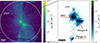 |
Fig. 1. Gas surface density map of the PONOS simulation (left panel). The dashed circle corresponds to the virial radius, Rvir. The right panel shows the [C II] line surface density map obtained using the fiducial model of Schimek et al. (2024a,b), which assumes solar elemental abundances, zoomed into the galaxy disc and the merging companions. |
The fiducial model from Schimek et al. (2024a) uses radiative transfer post-processing with KRAMSES-RT (Pallottini et al. 2019; Decataldo et al. 2019, 2020), to model the propagation of radiation from all emitting sources. KRAMSES-RT is a customised version of the adaptive mesh refinement (AMR) code RAMSES-RT (Teyssier 2002; Rosdahl et al. 2013) featuring a non-equilibrium chemical network generated by KROME (Grassi et al. 2014). For the post-processing, the SPH simulation was converted into an AMR grid (see Schimek et al. 2024a for details), with eight different refinement levels, resulting in grid sizes ranging from 1.52 pc for the high-density regions (higher resolution) to 195.3 pc for the low-density regions (lower resolution). Since the dynamical evolution is turned off in the RT post-processing, there is no mixing of the hot and cold gas. This can be seen in the bottom panels of Fig. 8 in Schimek et al. (2024a), where they show the density-temperature phase diagrams for their fiducial RT model. Schimek et al. (2024a) modelled the emission lines of PONOS using the 1D photoionisation code CLOUDY (Ferland et al. 2017), by first creating multidimensional CLOUDY grids and then interpolating to the values in the simulation cell. As the PONOS simulation does not trace elements directly for each particle, Schimek et al. (2024a,b) assumed solar abundances using the default CLOUDY setup (Grevesse & Sauval 1998; Holweger 2001; Prieto et al. 2001; Allende Prieto et al. 2002).
2.2. Post-processing with CLOUDY
To model the emission lines of PONOS, following the setup in Schimek et al. (2024a), we created a multidimensional grid consisting of individual CLOUDY models, using slab geometry. This type of grid modelling has been used in previous theoretical studies (e.g. Olsen et al. 2015, 2018; Pallottini et al. 2019, 2022; Katz et al. 2019, 2022; Lupi et al. 2020). Our grid consists of four parameters: temperature log(T) [K], density log(nH) [cm−3], metallicity log(Z) [Z⊙], and radiation field log(G0) [1.6 × 10⁻³ erg cm−2 s−1], where their maximum and minimum values are taken directly from the KRAMSES-RT post-processed simulation. When referring to the metallicity, we refer to the gas-phase metallicity, unless otherwise stated. Due to the post-processing with KRAMSES-RT, we kept the temperature in the CLOUDY models constant, similar to the fixed-temperature models in Lupi et al. (2020). Note that there are inconsistencies when combining KRAMSES-RT and CLOUDY in the post-processing, as KRAMSES-RT solves non-equilibrium photochemistry and CLOUDY assumes photoionisation equilibrium. However, when comparing different FIR modelling approaches for their simulated z = 6 galaxy, Lupi et al. (2020) found good agreement between their fixed-temperature CLOUDY models and the predictions from the non-equilibrium chemistry using KROME only.
The size range and abundance of dust were set to follow typical values for the local ISM, which reproduces the observed extinction properties of our galaxy, where we set the dust abundance and depletion of heavier elements to scale linearly with the Z parameter. With PONOS being a galaxy at z = 6.5, this could lead to an overestimation of the dust abundance where the metallicity is high; however, < 8% of the gas have super-solar metallicities. Since we only consider FIR emission lines in this work, we do not expect dust to have a significant effect in terms of dust attenuation of the emission lines, but we acknowledge that it can affect the amount of metals that emit the FIR emission lines. At z = 6.5, the CMB temperature is 20 K, which was included in the modelling. To compute the [C II], [O III], [N II] and [N III] line luminosities, considering the AMR structure in KRAMSES-RT, we integrated the emission from CLOUDY along the depth corresponding to the length of the AMR grid-cells and multiplied the integral with the area of the cell. We refer to Schimek et al. (2024a) for a more in-depth description of their fiducial model and the post-processing with KRAMSES-RT and CLOUDY.
2.3. Solar model with coarser grid
The fiducial model from Schimek et al. (2024a,b) has a grid consisting of 42 560 independent CLOUDY models. Since this is computationally expensive to run, we cut down the computational cost by reducing the number of grid points, allowing us to test multiple models. To make the grid coarser, we increased the step size in the temperature and density ranges, resulting in a total of 19 712 independent CLOUDY models. We list the final grid values for our coarser model in Table 1, where we added two additional high-temperature values (log(T) = 5.2, 5.7), hence changing the spacing of the original grid. This was done for more accurate [O III] treatment, as [O III] is more sensitive to higher gas temperatures. Such high temperatures are produced by supernovae feedback, which in PONOS is modelled following Stinson et al. (2006), where the cooling of hot and cold gas is delayed. However, the KRAMSES-RT post-processing allows gas with temperatures T ≤ 106 K to cool, while the cooling of warmer gas is artificially suppressed to take into account shock heating by stellar mechanical feedback, which is not in action without dynamical evolution. The temperatures included in our CLOUDY models, T = 102 − 106 K, are therefore not affected by the artificial cooling suppression (Stinson et al. 2006). To test the consistency with Schimek et al. (2024a), we reproduced their fiducial model with solar abundance ratios with the coarser grid. We find our coarser model to be overall consistent with Schimek et al. (2024a,b), with a change of ≲8% in total [C II], [O III] and [N II] luminosities compared to Schimek et al. (2024a,b). The [N III] luminosity is the most enhanced one compared to Schimek et al. (2024b), with a 50% higher total luminosity. This is due to our change in the temperature grid range compared to Schimek et al. (2024a), where we add two additional temperature values (log(T) = 5.7, 6.0). Hereafter we refer to this model as the Solar model, and use the same CLOUDY setup and grid values for the other non-solar models described in Sect. 3.
CLOUDY grid parameters.
3. Changing the elemental abundances
3.1. Observational constraints of the C/O and N/O abundance ratios
One of the proposed contributing factors to the observed high [O III]/[C II] luminosity ratio at z > 6 is a lower C/O abundance ratio (Harikane et al. 2020; Arata et al. 2020; Katz et al. 2022). In this work, we define abundance as the element abundance with respect to hydrogen, unless otherwise stated. Oxygen and other α-elements (i.e. Mg, Si, S, and Ca) are produced by massive stars (M ≳ 8 M⊙), and returned to the ISM through cc-SNe (Timmes et al. 1995; Kobayashi et al. 2006, 2020), which have relatively short timescales of ∼1 − 10 Myr (Kobayashi et al. 2006). Carbon is also produced by these massive stars, but a significant contribution to the carbon abundance is due to winds from low-mass (M ∼ 1 − 4 M⊙) asymptotic giant branch (AGB) stars, which have longer lifetimes of ≳100 Myr (Nomoto et al. 2013; Kobayashi et al. 2011, 2020). Nitrogen is mainly produced by intermediate-mass (M ∼ 4 − 7 M⊙) AGB stars, causing nitrogen to have a slightly longer formation timescale than carbon (Nomoto et al. 2013). In PONOS, the majority of the stellar particles are young (≤200 Myr), hence we do not expect many AGB stars. Although there may be some contribution from AGB stars, we expect cc-SNe to be the main enrichment mechanism in the simulation.
Due to the different formation timescales of carbon, nitrogen, and oxygen, assuming solar abundances would not be representative of the high-redshift Universe. In this work, we explore what effect does changing the elemental abundances in CLOUDY have on the resulting FIR line luminosity values and ratios. More specifically, we ran three non-solar models, which respectively assume C/O and N/O abundance ratios inferred from three different types of observational constraints: (i) JWST observations of a single, z > 6 galaxy; (ii) observations of local low-metallicity dwarf galaxies; and (iii) observations of metal-poor halo stars in the Milky Way. The observational results used in the three models are briefly described below, with the oxygen abundance and C/O and N/O abundance ratios summarised in Table 2.
C/O and N/O ratios used for the emission line modelling.
3.1.1. ‘High-z’ model using C/O and N/O measured at z > 6
The launch of JWST has enabled us to spectroscopically estimate the C/O and N/O abundance ratios at z > 6 (Arellano-Córdova et al. 2022; Jones et al. 2023; Isobe et al. 2023; Cameron et al. 2023; Topping et al. 2024). Our first non-solar model, hereby referred to as the ‘High-z’ model, uses the log(C/O) = − 1.01 estimated by Jones et al. (2023), which is ∼5 times lower than the solar ratio, for the z = 6.23 galaxy GLASS_150008 using rest-frame UV and optical OIII], CIII] and CIV emission lines detected with NIRSpec. This galaxy was observed as a part of the GLASS-JWST Early Release Science Program. GLASS_150008 is smaller than PONOS, with a stellar mass of M* ≈ 2.45 ⋅ 108 M⊙, and has a sub-solar oxygen abundance of log(O/H)+12 = 7.39. For this same source, Isobe et al. (2023) measured log(N/O) = − 0.40 using rest-frame UV NII] and NIV] lines, with C/O and O/H values in agreement with Jones et al. (2023). This super-solar nitrogen abundance is much higher than local measurements (Berg et al. 2016, 2019; Kojima et al. 2017); however, it is comparable to other recent super-solar N/O measurements at z > 6 (Cameron et al. 2023; Senchyna et al. 2024; Topping et al. 2024). With the currently small numbers of C/O and N/O abundance ratios measurements at z > 6, GLASS_150008 may be an outlier and not representative of the general high-z population. We emphasise this because of the high N/O abundance ratio, given that such high nitrogen abundances would be expected in high-metallicity systems (Vincenzo et al. 2016).
3.1.2. Dwarfs model using C/O and N/O from local dwarf galaxies
An alternative to studying high-redshift galaxies directly is to use more accessible local analogues. High-redshift galaxies are observed to be smaller and less settled, with low metallicities, which are conditions observed in low-metallicity dwarf galaxies. In this second non-solar model, which we hereby refer to as the Dwarfs model, we used the C/O and N/O abundance ratios from the combined sample of 40 metal-poor dwarf galaxies from Berg et al. (2019), with smaller masses compared to PONOS of M* = 106 − 108 M⊙. Berg et al. (2019) estimated average values of log(C/O) = − 0.71 and log(N/O) = − 1.46, with an average oxygen abundance of log(O/H)+12 = 7.85 for this sample, using detections of the UV O+2 and C+2 collisionally excited lines obtained from the Hubble Space Telescope (HST) and optical N+ lines from the Sloan Digital Sky Survey (SDSS).
3.1.3. Halo model using C/O from metal-poor halo stars
Our third model, which we hereafter refer to as the Halo model, adopts the carbon and oxygen abundances from low-metallicity, high-alpha halo stars in the Milky Way. The abundances were estimated by Nissen et al. (2014), using the sample of halo stars from Nissen & Schuster (2010) from measurements of optical spectra from the Very Large Telescope (VLT) and the Nordic Optical Telescope (NOT). High-alpha stars have a higher abundance of alpha elements compared to the iron abundance and are thought to be enriched by cc-SNe only (Schuster et al. 2012). We selected the nine high-alpha stars with the lowest oxygen abundances, corresponding to the plateau in Fig. 12 of Nissen et al. (2014), showing C/O versus O/H for their stellar samples. These halo stars have average log(O/H) +12 = 8.02 and log(C/O) = − 0.65, where we have converted the solar-normalised logarithmic abundances2 in Nissen et al. (2014) using their non-LTE corrected derived solar abundances in their Table 1. Nitrogen abundance measurements are not available for this sample, hence this model is not included in the investigation of the [N II] and [N III] lines.
3.2. Implementation in CLOUDY
As we used the metals command in CLOUDY to specify the metallicity, the code assumes a default solar mixture (Grevesse & Sauval 1998; Holweger 2001; Prieto et al. 2001; Allende Prieto et al. 2002) for its photoionisation modelling, scaling it with the scale factor given as an input value (see CLOUDY documentation Hazy1, 7.10). To change abundances within the CLOUDY models, we used the element abundance command, allowing us to specify the abundance of specific elements relative to hydrogen. Since the metallicities of the sources from Jones et al. (2023), Berg et al. (2019), and Nissen et al. (2014) are lower than solar, it is necessary to scale the carbon, nitrogen, and oxygen abundances to a solar level, to ensure that the element abundances are then scaled correctly for the CLOUDY models. We relate the oxygen abundances from Jones et al. (2023) (used in the High-z model) and from Berg et al. (2019) (used in the Dwarfs model) to Z/Z⊙ using the relation from Ma et al. (2016),
 (1)
(1)
where Z⊙ = 0.02. Equation (1), which we used to scale the oxygen abundances to solar level, assumes a higher solar metallicity value than in CLOUDY. Because of this, we get an enhancement in oxygen abundance, which will boost the [O III] emission. We do not expect this light boost of [O III] to have an effect on the [O III]/[C II] and [O III]/[N II] ratios, as the input carbon and nitrogen abundances are set using the C/O and N/O abundance ratios. The line emissions scale almost linearly with the element abundances, so the luminosity ratios should not be significantly affected, which we discuss further in Sect. 5.5.
Using Eq. (1) results in a metallicity of log(Zgas/Z⊙) = − 1.61 for the high-z galaxy in Jones et al. (2023), related to its measured O/H value. We get log(Zgas/Z⊙) = − 1.15 for the dwarf galaxies in Berg et al. (2019) related to their measured average oxygen abundance. Using the log(Zgas/Z⊙) ratios, we then estimate what the oxygen abundance would be at solar metallicity, which is then used as the input oxygen abundance. At solar metallicities, this results in an input oxygen abundance of log(O/H) = − 3.0 for the High-z model and the Dwarfs model. For the Halo model, since we used measured abundances from stars and not galaxies, we used the relation between the iron abundance and the stellar metallicity from Ma et al. (2016),
![Mathematical equation: $$ \begin{aligned}{[\mathrm{Fe/H} ]} = \log (Z_{*}/Z_{\odot }) - 0.2 , \end{aligned} $$](/articles/aa/full_html/2025/10/aa52718-24/aa52718-24-eq2.gif) (2)
(2)
resulting in a metallicity of log(Z*/Z⊙) = − 1.035. We used the same method of scaling the oxygen abundance, resulting in an input abundance of log(O/H) = − 2.95 at solar metallicities for the Halo model. Since Eq. (2) relates the iron abundance to the stellar metallicity, while Eq. (1) relates the oxygen abundance to the gas-phase metallicity, we get a different input oxygen abundance for the Halo model when scaling the measured O/H ratio for the halo stars. The carbon and nitrogen abundances for the High-z, Dwarfs and Halo models were then calculated using the C/O and N/O ratios of the models, based on the input oxygen abundance. The relative abundances of the elements in the individual CLOUDY models are constant, assuming a uniform distribution of elements, similar to the models used by Olsen et al. (2017), Katz et al. (2022), Pallottini et al. (2022) and the fixed-temperature CLOUDY models in Lupi et al. (2020). We assume uniform distribution of elements since we are not tracing the evolution of the carbon, nitrogen, and oxygen abundances directly for each cell in the simulation. At z = 6.5, the main enrichment is due to cc-SNe, since the stellar particles are young (< 200 Myr old). We therefore do not expect many AGB stars in the simulation, making the effect of the non-uniform heavier element distribution negligible. Additionally, for a low-mass galaxy (M* = 2 × 10⁹ M⊙) such as PONOS, the gas is mixed by mergers and supernovae feedback. This results in a flat metallicity gradient (slope > − 0.1 [dex/kpc]) in the star-forming galactic disc, which is in agreement with observed estimates of similar-mass galaxies at z > 6 (Venturi et al. 2024; Garcia et al. 2025).
It is important to note that we did not change the intrinsic metallicity of PONOS itself, only the elemental abundances in CLOUDY. Nevertheless, changing the elemental abundances affects the line luminosities and, consequently, the luminosity ratios.
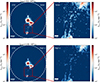 |
Fig. 2. [C II] line emission maps obtained with the Solar model (top panels) and the High-z model (bottom panels). The right panels are zoomed-in images of the tidal tail between merger B and merger A. The white dashed circles mark the extent of Rvir of PONOS. The line emission maps obtained with the Dwarfs and Halo models are shown in Appendix B. |
4. Results
4.1. Line luminosities
The resulting total [C II], [O III], [N II], and [N III] line luminosities from the PONOS halo, obtained by our four models (including the solar one), are listed in Table 3. The table also lists separately the contribution from the brightest ISM components that are due to the main disc and the closest merging companion (merger B, see Fig. 1).
The total [C II] line luminosity in the High-z model is a factor of 2.3 times lower compared to the Solar model, while the [O III] luminosity is ∼2 times higher than the Solar model luminosity. This results in a [O III]/[C II] luminosity ratio of 0.77, which is 4.5 times higher than the Solar model ratio of 0.17. The total [N II] and [N III] luminosities from the High-z model are both enhanced by a factor ∼5 compared to the Solar model. This results in the High-z model obtaining a [O III]/[N II] ratio of 1.3, which is lower than the Solar model ratio by a factor of 2.3.
The Dwarfs and the Halo models produce total [C II] luminosity values that are not too dissimilar from the Solar model, and [O III] luminosities that are higher by a factor of ∼2. This results in very similar [O III]/[C II] luminosity ratios equal to 0.40 and 0.37 respectively for these two models. The [N II] and [N III] luminosities obtained with the Dwarfs model are both ∼2.4 times lower compared to the Solar model luminosities, and the resulting [O III]/[N II] ratio becomes very high, ∼15.
In general, our non-solar models display [C II] luminosity values that are consistent with or slightly lower than the Solar model, but they all show an increased [O III] luminosity, resulting in higher [O III]/[C II] ratios compared to the Solar model. In terms of the nitrogen lines, we find large discrepancies of an order of magnitude between the total [N II] and [N III] luminosities in the High-z and Dwarfs models, which results in vastly different [O III]/[N II] ratios.
The contributions from the main disc and merger B components seem to be more or less constant between all four models, which is expected since we change the element abundances according to the same abundance ratios, hence not treating the ISM and CGM components differently.
4.2. Line emission maps
To examine any spatial variations in the line emissions that are due to the adoption of different elemental abundances, we produced [C II], [O III], [N II] and [N III] line maps with the four models. Since both the [N II] and [N III] lines trace ionised gas, we only show the [N II] maps here; however, the analysis of [N II] is applicable to [N III].
In Fig. 2 we compare the [C II] line emission maps obtained with the Solar model (top panels) and High-z model (bottom panels). The weaker [C II] emission seen in the High-z model map reflects its overall lower [C II] line luminosity compared to the Solar model. The High-z model [C II] map shows a lower surface brightness in the central ISM components of the disc and merger B, as well as lower extended emission in the tidal tails (and so, lower emission from CGM components). The Dwarfs and Halo model [C II] maps are shown in Appendix B: the former shows a slightly weaker emission compared to the Solar model, while the latter is more similar to the Solar model map.
In Fig. 3 we show the [O III] line emission maps for the Solar model (top panels) and the High-z model (bottom panels). The High-z model shows a higher [O III] surface brightness in the central ISM regions and stronger extended emission compared to the Solar model. This reflects the higher total [O III] luminosity in the High-z model. We find similar results for the Dwarfs and Halo models [O III] maps in Appendix B.
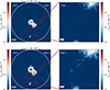 |
Fig. 3. [O III] line emission maps obtained with the Solar model (top panels) and the High-z model (bottom panels). The right panels are zoomed-in images of the tidal tail between merger B and merger A. The white dashed circles mark the extent of Rvir of PONOS. The line emission maps obtained with the Dwarfs and Halo models are shown in Appendix B. |
In Fig. 4 we compare the [N II] line emission maps obtained with the Solar (top panels), High-z (middle panels), and Dwarfs (bottom panels) models. The [N II] surface brightness in the High-z model map is significantly higher in the ISM compared to the Solar model map, in addition to exhibiting stronger extended emission. The Dwarfs model map shows the opposite trend, with a lower central [N II] surface brightness and much weaker extended emission compared to the Solar model. The large discrepancy in total [N II] luminosity between the High-z and Dwarfs models is reflected in their vastly different [N II] maps.
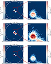 |
Fig. 4. [N II] line emission maps obtained with the Solar model (top panels), the High-z model (middle panels), and the Dwarfs model (bottom panels). The right panels are zoomed-in images of the main disc and surrounding area. The white dashed circles mark the extent of Rvir of PONOS. |
4.3. [O III]/[C II] ratio maps
Before computing the [O III]/[C II] ratio maps, we masked out the weak emission for both [O III] and [C II] by setting a minimum line surface brightness threshold of Σline < 1 L⊙ kpc−2, which is low and has a negligible effect on the total luminosity ratio value, as discussed in Schimek et al. (2024a). This allows us to focus our study of the [O III]/[C II] ratio on the brightest ISM components of PONOS, that is the main disc and merger B, which account for ≳80% of the total line luminosities (see Table 3).
Total [C II], [O III], [N II], and [N III] line luminosities.
In Fig. 5 we show the [O III]/[C II] line ratio maps obtained from the Solar model (left panel) and the High-z model (right panel). The factor 4.5 higher [O III]/[C II] luminosity ratio obtained by the High-z model is clearly reflected in the ratio maps. The distribution of the high-ratio and low-ratio regions in both the Solar model map and the High-z model map occur at the same locations. This is expected from the modelling, as we change the carbon and oxygen abundances according to the same C/O ratio for all individual CLOUDY models in each grid. The Dwarfs model and Halo model ratio maps in Appendix B reflect their higher luminosity ratios compared to the Solar model, in addition to showing the same spatial distributions as the Solar model map. The luminosity ratio in the High-z, Dwarfs and Halo models all seem to change uniformly throughout the maps.
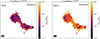 |
Fig. 5. Surface brightness ratio maps of the [O III]/[C II] luminosity ratio, comparing the Solar model (left panel) and the High-z model (right panel). The title above each panel gives the total luminosity ratios. The ratio maps obtained with the Dwarfs and Halo models are shown in Appendix B. |
5. Discussion
In this section, we discuss our results and compare them with previous observational and theoretical works.
5.1. The [O III]/[C II] luminosity ratio
In Fig. 6 we show the [O III]/[C II] luminosity ratio as a function of SFR obtained from our High-z model (red), together with the value obtained by Schimek et al. (2024a) by adopting solar abundances (purple). The top panel compares our results to observations of z > 6 galaxies and local analogues, while the bottom panel shows our results compared to other theoretical efforts. We show only the High-z model out of our three non-solar models because it is the one producing the highest [O III]/[C II] values.
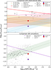 |
Fig. 6. Total [O III]/[C II] line luminosity ratio as a function of SFR for the High-z model (red) and Schimek et al. (2024a,b) (purple). The top panel reports the comparison with observational data from Hashimoto et al. (2019) at z ∼ 7, Witstok et al. (2022) at z = 6.7 − 7, Carniani et al. (2020) at z ∼ 6 − 9, missing [C II] flux corrected values from Carniani et al. (2020) (SBD corr.) at z ∼ 6 − 9, Harikane et al. (2020) at z ∼ 6, Ren et al. (2023) at z = 7.2, Algera et al. (2024) at z = 7.3, Bakx et al. (2020) at z = 8.31, Laporte et al. (2017) at z = 8.3, Fujimoto et al. (2024) at z = 8.5 (lower limit), and Schouws et al. (2025a,b) at z = 14.2 (lower limit). The relations included are the z = 6 − 9 relation from Harikane et al. (2020), the best-fit relation from Pallottini et al. (2022), and the high-redshift, local dwarfs, and local starbursts (SBs) relations from De Looze et al. (2014). The bottom panel reports the comparison with simulation studies by Katz et al. (2022) (z = 6), Ramos Padilla et al. (2023) (z = 6), Pallottini et al. (2022) (z = 7.7), and Lupi et al. (2020) (z = 6). The relations are from Arata et al. (2020) (z = 6 − 9) and Olsen et al. (2017) (z ≃ 6). |
Focusing on the top panel, our High-z model delivers a [O III]/[C II] ratio that is a factor of 4.5 higher than the ratio from Schimek et al. (2024a), and so it is closer to the observed z > 6 data. Furthermore, the High-z model is in good agreement with the high-redshift (z = 0.5 − 6.6) and local (z < 0.5) metal-poor dwarf relations from De Looze et al. (2014). However, despite the improvement, the High-z model is still falling short of most of the [O III]/[C II] luminosity ratios observed at z > 6, most notably it is a factor of 13 lower than the z = 6 − 9 estimates from Harikane et al. (2020). The discrepancy with the observations is reduced significantly if comparing the High-z model ratio to the Pallottini et al. (2022) relation: a best-fit relation of the z = 6 − 9 observational data from Carniani et al. (2020) that corrects for missing [C II] flux, i.e. surface brightness dimming (SBD), at low SFR. For what concerns the individual [C II] and [O III] line luminosities, the High-z model is in very good agreement with observational data on the [C II]-SFR relation, while it sits below most of the data points on the observed [O III]-SFR relation (see plots reported in the Appendix A). We note that most of the available observational constraints are for sources at higher SFRs than PONOS. As there is only a small sample of [O III] observations compared to [C II], it is possible that the observed [O III]/[C II] luminosity ratios are biased towards the brightest [O III]-emitters (Bakx et al. 2024).
Focusing on the bottom panel, we compute a lower ratio than Ramos Padilla et al. (2023) and are barely outside the scatter of Olsen et al. (2017), which is likely due to them producing significantly lower [C II] emission at the comparable SFR (see Fig. A.1). The High-z model is close to the z = 6 − 9 simulated estimates from Arata et al. (2020), who track the carbon and oxygen abundances for each particle and include enrichment from cc-SNe, Type Ia SNe and AGB stars. This way, the enrichment timescales for carbon and oxygen are included more accurately. Our modelling is in very good agreement with the z = 6 data from Katz et al. (2022) (with a spatial resolution of 7.3 pc h−1 similar to the PONOS simulation), at comparable SFR. The agreement in [O III]/[C II] ratio values is expected, as we in this work apply a low C/O abundance ratio from observational constraints consistent with assumptions of pure cc-SNe enrichment (Jones et al. 2023). Comparing the [C II]-SFR and [O III]-SFR relations at similar SFR as PONOS, Katz et al. (2022) line luminosities are lower than what we obtain from our High-z model (see Fig. A.1 and Fig. A.2).
5.2. The C/O abundance ratio and metallicity as contributing factors to the [O III]/[C II] ratio
With the lowest C/O abundance ratio of all our models, the High-z model obtained the highest [O III]/[C II] ratio. The trend of increasing [O III]/[C II] ratio for lower C/O abundance values is consistent with the theoretical predictions from Katz et al. (2022) and Arata et al. (2020). Arata et al. (2020) also found that the C/O ratio decreases at higher redshifts. Harikane et al. (2020) found, however, using CLOUDY modelling, that lower C/O abundances can only partially explain the highest [O III]/[C II] luminosity ratios observed at z > 6.
To further explore the significance of including a physically motivated C/O abundance ratio, we plot in Figure 7 the [O III]/[C II] luminosity ratios obtained from our models as a function of the average intrinsic metallicity of PONOS, and compare them with the [O III]/[C II]-metallicity relation from Arata et al. (2020) (grey dashed line),
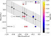 |
Fig. 7. [O III]/[C II] luminosity ratio vs. metallicity Z/Z⊙ in PONOS. Our models are colour-coded based on the assumed C/O abundance ratios. The circle symbols correspond to the luminosity ratios and average metallicities computed for the whole simulated halo (log(Z/Z⊙) = − 0.55). The diamonds show the contribution from the main disc and merger B component only (log(Z/Z⊙) = − 0.22). The grey dashed line is the best-fit relation from Arata et al. (2020) for their simulated sample of z = 6 − 9 galaxies, with the grey area corresponding to their ≲0.2 dex dispersion. The grey symbols are the PONOS models shifted to the metallicity values expected from the Arata et al. (2020) relation. |
![Mathematical equation: $$ \begin{aligned} \log (Z/Z_{\odot }) = -0.37 - 0.52\log ([\mathrm{O}\,\text{ iii}]/[\mathrm{C}\,\text{ ii}]). \end{aligned} $$](/articles/aa/full_html/2025/10/aa52718-24/aa52718-24-eq3.gif) (3)
(3)
Equation (3) is a best-fit relation derived by Arata et al. (2020) using their simulated z = 6 − 9 sample with luminosity ratios − 0.5 < log(O III]/[C II]) < 2.0. Arata et al. (2020) were motivated by the need for estimating the observed gas-phase metallicities at high redshifts without using iron tracers that do not consider the enhancement of α-elements in early galaxy evolution. As explained above, our methodology consists of changing the element abundances in CLOUDY, and so all models share the same intrinsic metallicity of the PONOS simulation, equal to log(Z/Z⊙) = − 0.55 (circles in Fig. 7), and an average metallicity of log(Z/Z⊙) = − 0.22 when considering only the main disc and merger B, i.e. removing the more extended CGM components and the merger A (diamonds in Fig. 7). The colour coding in Fig. 7 corresponds to the C/O abundance ratios in our models and the grey symbols represent the metallicities of our models extrapolated from the [O III]/[C II] luminosity ratios by assuming the relation by Arata et al. (2020). Compared to the other models, we find that the High-z model is in better agreement with the expectations from the Arata et al. (2020) relation, and it is perfectly consistent with this relation when considering only the main disc and merger B. Therefore, we can conclude that using a C/O abundance ratio from observations of a z > 6 galaxy produces [O III]/[C II] luminosity ratios that are more consistent with the intrinsic metallicity of PONOS.
5.3. The ionisation parameter as a contributing factor to the [O III]/[C II] ratio
The High-z model estimates a lower [O III] line luminosity than high-redshift observations and theoretical modelling efforts from Arata et al. (2020) at comparable SFR (see e.g. Fig. A.2), which may contribute to the fact that the [O III]/[C II] luminosity ratio is still lower than most observations at z > 6. For their simulations, Arata et al. (2020) estimate high ionisation parameters of −2.2 ≲ log(U)≲ − 1.5, consistent with recent high-redshifts observations (Bunker et al. 2023; Topping et al. 2024; Fujimoto et al. 2024). Higher ionisation parameters have also been discussed as contributing factors to the enhanced [O III]/[C II] luminosity ratio in observational studies (Harikane et al. 2020). For comparison with these works, we estimate the log(U) value of PONOS using the volume-average estimate from Hirschmann et al. (2017):
 (4)
(4)
where Qion is the rate of ionising photons which we take from the RT post-processed simulation,  is the hydrogen number density in H II-regions used in Hirschmann et al. (2017), ϵ = ngas/nH, * is the filling factor, and αB is the case-B hydrogen recombination coefficient. For the whole galaxy halo, we estimate log(U) = − 2.6, and for the main disc and merger B components, we estimate log(U) = − 2.45. These are lower than what was estimated by Arata et al. (2020) for their sample, hence consistent with the hypothesis that a higher ionisation parameter would result in a higher [O III] luminosity. Using CLOUDY models, Harikane et al. (2020) found high ionisation parameters of log(U) = − 1 to reproduce their highest [O III]/[C II] ratios, which is significantly higher than our log(U) estimate for PONOS, even when we consider only the main disc and merger B. Similarly high parameters have been found in observations by Topping et al. (2024) for a z ≈ 6 galaxy. From observations of GN-z11 at z = 10.6, Bunker et al. (2023) computed log(U) = − 2.25, which is only a factor of ∼2 higher than PONOS.
We thus conclude that higher ionisation parameters resulting from extreme high-redshift environments, for example top-heavy initial mass functions, or spectral energy distributions with harder radiation fields, could contribute to enhancing the [O III]/[C II] luminosity ratio further.
5.4. The nitrogen lines and the [O III]/[N II] ratio
Observations of [N II] and [N III] at z > 6 are very limited (see Figure 8), resulting in a lack of observational constraints adequate to test the results of our models. Nevertheless, it is interesting to explore further the [O III]/[N II] ratio because of its potential as a metallicity tracer at high-z (Nagao et al. 2011; Pereira-Santaella et al. 2017; Rigopoulou et al. 2018).
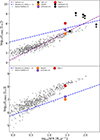 |
Fig. 8. Total [N II] luminosity (top panel) and [N III] luminosity (bottom panel) as functions of SFR for the High-z model (red), Dwarfs model (orange), and Schimek et al. (2024a,b) (purple). Both panels include comparisons with the simulated z = 6 sample from Ramos Padilla et al. (2023) (grey circles) and the linear relations from Mordini et al. (2021) based on observations of galaxies in the local Universe. In the top panel we include the [N II] observation from Killi et al. (2023) (black circle) at z ∼ 7, the observed upper limits from Harikane et al. (2020) at z ∼ 6 and Sugahara et al. (2021) at z ∼ 7 (black circles with arrows), and the theoretical relation from Kannan et al. (2022) (z = 6 − 10). |
In the top panel of Fig. 8 we plot the total [N II] line luminosity as a function of SFR obtained by our High-z (red) and Dwarfs (orange) models and Schimek et al. (2024a,b) (purple). For comparison with observations, we include the z ∼ 7 observation from Killi et al. (2023) (black circle), which is the first detection of [N II] in a non-quasar galaxy at z > 6, and the observed upper limits at z > 6 from Harikane et al. (2020) and Sugahara et al. (2021) (black circles with arrows). Due to the lack of high-redshift observations, we have also included the relation from Mordini et al. (2021) based on observations of local star-forming galaxies (SFG), where we adopted the Kennicutt & Evans (2012) conversion between LIR and SFR similar to Ramos Padilla et al. (2023). In the same panel, we include the z = 6 simulations from Ramos Padilla et al. (2023) (grey circles) and the theoretical relation from Kannan et al. (2022). Both Ramos Padilla et al. (2023) and Kannan et al. (2022) have resolutions at mgas ≥ 105 M⊙, significantly lower than PONOS. The total [N II] luminosity resulting from the High-z model, for which we adopted log(N/O) = − 0.40 (Isobe et al. 2023), is higher than the z ∼ 7 observational constrain from Killi et al. (2023) and the relation from Mordini et al. (2021) at comparable SFR to PONOS. The total [N II] luminosity is also higher than the theoretical predictions from Ramos Padilla et al. (2023) and Kannan et al. (2022) at comparable SFR. We stress that the super-solar N/O abundance ratio adopted in the High-z model is based on recent JWST observations of a single z > 6 galaxy (Isobe et al. 2023), which might not be representative of the broader population of high-redshift galaxies. Recent z > 6 data from JWST have uncovered a few surprisingly high N/O abundance ratios (Cameron et al. 2023; Senchyna et al. 2024; Topping et al. 2024); however, the origin of these high abundance ratios is still unknown. Our predictions from the Dwarfs model, with sub-solar log(N/O) = − 1.46 (Berg et al. 2019), and the prediction from Schimek et al. (2024a), are in better agreement with the observational data from Killi et al. (2023) and Mordini et al. (2021). The Dwarfs model and the fiducial Solar model by Schimek et al. (2024a) are also consistent with the theoretical estimates from Ramos Padilla et al. (2023) and Kannan et al. (2022).
In the bottom panel of Fig. 8 we plot the total [N III] line luminosities as functions of SFR for our High-z model (red), Dwarfs model (orange) and Schimek et al. (2024a) (purple). We include a relation from Mordini et al. (2021) based on local Active Galactic Nucleus (AGN) observations, again adopting the Kennicutt & Evans (2012) conversion. We compare to AGN data, as there are no available non-AGN emission line measurements. For theoretical comparison, we have included the z = 6 simulations from Ramos Padilla et al. (2023) (grey circles). We find that the total [N III] luminosity obtained by our High-z model is in very good agreement with the Ramos Padilla et al. (2023) simulations at comparable SFR, while the lower values from the Dwarfs model and from Schimek et al. (2024a) agree with the local relation from Mordini et al. (2021). We remind that, the total [N III] luminosity in our Solar model is ∼50% higher than in Schimek et al. (2024a) due to the addition of high-temperature (log(T) = 5.7, 6.0) grid values in CLOUDY (see Sect. 2.3). Therefore, our [N III] predictions should be considered as upper limits.
Comparing our results from the top and bottom panels of Fig. 8, we find that none of our models agrees with both the [N II]-SFR and [N III]-SFR relations predicted by Ramos Padilla et al. (2023). Due to the small sample of nitrogen line observations available at high-z, the question regarding the behaviour of the [N III]-SFR relation in the early Universe remains open.
Since O++ and N+ have critical densities of 510 cm−3 and 310 cm−3 respectively, the [O III]/[N II] ratio has a low dependence on the ISM gas density. However, this luminosity ratio is highly dependent on the ionisation parameter. In Fig. 9, we show the [O III]/[N II] ratio as a function of the intrinsic metallicity of PONOS for the solar (yellow-green), High-z (red) and Dwarfs (orange) models. The circles show the contribution from the whole galaxy halo, while the diamonds consider only the brightest components (main disc and merger B). For comparison, we have included the theoretical predictions from Pereira-Santaella et al. (2017), where each shaded region corresponds to a model assuming a specific ionisation parameter: log(U) = − 4, −3.5, −3, −2.5 and −2. The width of the shaded regions spans the density range: log nH (cm−3) = 1 − 4, showing the low dependence on gas density. For comparison to observations, we include the z ∼ 7 observation from Killi et al. (2023). We find that the large discrepancy in [N II] luminosity between the High-z model and the Dwarfs model, results in vastly different [O III]/[N II] ratios. This is the result of the different N/O abundance ratios assumed.
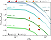 |
Fig. 9. [O III]/[N II] as a function of metallicity Z [Z⊙] for the Solar model (yellow-green), High-z model (red) and Dwarfs model (orange). The circles show the contribution from the whole galactic halo, while the diamonds consider only the main disc and merger B. The shaded regions are the model predictions of the [O III]/[N II] ratio as functions of metallicity from Pereira-Santaella et al. (2017), with each shaded region corresponding to a model assuming a certain ionisation parameter: log(U) = − 4, −3.5, −3, −2.5 and −2. The width of the shaded regions spans the density range: log(nH) = 1 − 4. The grey star represents the observed ratio from Killi et al. (2023) at z ∼ 7. |
From Fig. 9, it is clear that our models produce [O III]/[N II] luminosity ratios well below what would be expected from the Pereira-Santaella et al. (2017) predictions considering the ionisation parameter of PONOS. The very low luminosity ratio obtained by the High-z model is due to the observed super-solar N/O ratio (Isobe et al. 2023) assumed in our modelling. We emphasise again that recent observations of z > 6 galaxies have found excess nitrogen that is not trivial to explain (Cameron et al. 2023; Isobe et al. 2023; Topping et al. 2024), and we need more observational data of the [N II] emission line at high redshifts to further constrain the [O III]/[N II] ratios.
5.5. Other effects on the far-infrared luminosity ratios
The [O III]/[C II] luminosity ratio obtained by the High-z model is 4.5 times higher than the ratio obtained by the Solar model, while the C/O abundance ratio used as input for the High-z model is 5.1 times lower than the input C/O in the Solar model. While the difference between the ratios is small (∼10%), it shows that the line luminosities scale close to linear with the element abundance. However, there is something else affecting the line luminosities. Similar discrepancies between emission line ratios and abundance ratios were found by McClymont et al. (2024), who modelled optical emission lines arising from the diffuse ionised gas (DIG) in a simulated Milky Way-like galaxy. McClymont et al. (2024) found that the relative abundance ratios were not enough to explain the behaviour of the optical line ratios.
We investigated a few selected CLOUDY models from our four models separately, focusing on how the relative line emissions as functions of depth behave compared to what we expect from the relative element abundances. Focusing on the [O III] line, we found that for low-density (n = 1 cm−3), high-temperature (T = 104 K) CLOUDY models, the relative emission obtained by the High-z, Dwarfs and Halo models with respect to the Solar model, is slightly lower than expected, especially at depths corresponding to length of the smallest AMR grid cells. At the same temperature, but higher densities (n = 100 cm−3), we find the relative [C II] emission to be higher than expected, especially for the Dwarfs and High-z models. These discrepancies increase with increasing gas-phase metallicities Z, as more metals are present in the gas. Furthermore, the depths at which the discrepancies are the highest decrease with increasing metallicity, which could be related to the PDR column density being proportional to 1/Z (Kaufman et al. 2006; Harikane et al. 2020; Katz et al. 2022), and thus, the interface between the H II regions and PDRs is shifted. Since the line luminosities are computed considering the AMR structure in KRAMSES-RT (Sect. 2.2), the non-uniform scaling of the emission along the depth of the slabs affect the total line luminosities.
Note that we have only investigated a small sample of different parameters in our CLOUDY models, and the discrepancy between the [O III]/[C II] luminosity ratio and the C/O abundance ratio is small. While analysis of other parameters would be necessary to further investigate the discrepancy amongst the FIR lines, it is beyond the scope of this work.
6. Conclusions
In this work, we investigated the reasons behind the high [O III]/[C II] luminosity ratios measured in high-redshift galaxies, which are significantly higher (ratios of 1–20) compared to the local Universe (ratios of ≤1). Additionally, we modelled the FIR nitrogen lines and studied the [O III]/[N II] ratio, which is a potential metallicity tracer. We modelled FIR emission lines with CLOUDY for the high-resolution PONOS (Fiacconi et al. 2017; Schimek et al. 2024a,b), changing elemental abundance ratios to be more representative of the chemical composition found in high-redshift galaxies. We explored different input C/O and N/O abundance values, basing our assumptions on (i) JWST observations of a single high-z galaxy (Jones et al. 2023; Isobe et al. 2023), (ii) local low-metallicity dwarf galaxy analogues (Berg et al. 2019), and (iii) observations of metal-poor halo stars in the Milky Way (Nissen et al. 2014). Our main results can be summarised as follows:
-
Reducing the log(C/O) abundance ratio by a factor of 5.1 (High-z model) increases the [O III]/[C II] luminosity ratio by a factor of 4.5 when compared to assuming solar abundances. Additionally, our obtained total [C II] and [O III] luminosity values are consistent with and closer to observations and simulations with similar SFR as PONOS. This shows why it is important to consider the chemistry of high-redshift galaxies when modelling their emission lines.
-
The [O III]/[C II] luminosity ratio we obtain when assuming a high-redshift log(C/O) abundance ratio, is closer to the luminosity ratio that we would expect based on the intrinsic metallicity of PONOS, assuming the theoretical [O III]/[C II]-Z relation by Arata et al. (2020).
-
Our models produce [O III]/[N II] ratios that are lower than what we expect from current theoretical models, considering the ionisation parameter we calculated for PONOS.
-
The large discrepancy in the N/O abundance ratios used as input in our models, from observations of a z > 6 galaxy and local dwarf galaxies, resulted in vastly different [O III]/[N II] luminosity ratios and total [N II] and [N III] luminosity values. Nevertheless, we obtain total luminosity values that agree with the few observational and theoretical constraints at similar SFR as PONOS.
-
Small non-linearities between the total line luminosities and the element abundances could hint towards a complex interplay of the chemistry and other ISM properties.
Our results highlight the importance of further improving and developing theoretical models of FIR and sub-mm line emission from high-z galaxies. These modelling efforts need to be coupled with high-resolution zoom-in cosmological simulations that resolve the physical processes and the small scales that are relevant to the cold and warm phase traced by FIR and sub-mm lines, not only on the ISM but also in the CGM, where a significant fraction of the [C II] emission can arise (see also Schimek et al. 2024a). These efforts are urgently needed to inform ongoing ALMA follow-ups of the increasing number of z > 6 galaxies that are being discovered and, in the future, to interpret the wide-field, high-sensitivity line observations and surveys that will be performed by AtLAST (see Mroczkowski et al. 2025 for the telescope design, and van Kampen et al. 2024 and Lee et al. 2024 for the science drivers relevant to this study).
Under development, consult: https://www.atlast.uio.no/
Similarly to Nissen et al. (2014), we refer to solar-normalised logarithmic ratios as the difference between the logarithmic stellar abundance ratio and the solar abundance ratio, i.e. [C/O] ≡ log(C/O)star − log(C/O)Sun.
Acknowledgments
This project has received funding from the European Union’s Horizon Europe and Horizon2020 research and innovation programmes under grant agreements No. 101188037 (AtLAST2) and No. 951815 (AtLAST). Views and opinions expressed are however those of the author(s) only and do not necessarily reflect those of the European Union or European Research Executive Agency. Neither the European Union nor the European Research Executive Agency can be held responsible for them. C.T acknowledges support from the Knut and Alice Wallenberg Foundation. The simulations were performed using the resources from the National Infrastructure for High Performance Computing and Data Storage in Norway, UNINETT Sigma2, allocated to Project NN9477K. We acknowledge the use of the programming language Python (Van Rossum & Drake 1995, 2009) and packages: NumPy (van der Walt et al. 2011), Matplotlib (Hunter 2007) and Pynbody (Pontzen et al. 2013).
References
- Algera, H. S. B., Inami, H., Sommovigo, L., et al. 2024, MNRAS, 527, 6867 [Google Scholar]
- Allende Prieto, C., Lambert, D. L., & Asplund, M. 2002, ApJ, 573, L137 [NASA ADS] [CrossRef] [Google Scholar]
- Arata, S., Yajima, H., Nagamine, K., Abe, M., & Khochfar, S. 2020, MNRAS, 498, 5541 [NASA ADS] [CrossRef] [Google Scholar]
- Arellano-Córdova, K. Z., Berg, D. A., Chisholm, J., et al. 2022, ApJ, 940, L23 [CrossRef] [Google Scholar]
- Bakx, T. J. L. C., Tamura, Y., Hashimoto, T., et al. 2020, MNRAS, 493, 4294 [NASA ADS] [CrossRef] [Google Scholar]
- Bakx, T. J. L. C., Algera, H. S. B., Venemans, B., et al. 2024, MNRAS, 532, 2270 [Google Scholar]
- Berg, D. A., Skillman, E. D., Henry, R. B. C., Erb, D. K., & Carigi, L. 2016, ApJ, 827, 126 [NASA ADS] [CrossRef] [Google Scholar]
- Berg, D. A., Erb, D. K., Henry, R. B. C., Skillman, E. D., & McQuinn, K. B. W. 2019, ApJ, 874, 93 [NASA ADS] [CrossRef] [Google Scholar]
- Bradač, M., Garcia-Appadoo, D., Huang, K.-H., et al. 2017, ApJ, 836, L2 [Google Scholar]
- Brauher, J. R., Dale, D. A., & Helou, G. 2008, ApJS, 178, 280 [NASA ADS] [CrossRef] [Google Scholar]
- Bunker, A. J., Saxena, A., Cameron, A. J., et al. 2023, A&A, 677, A88 [NASA ADS] [CrossRef] [EDP Sciences] [Google Scholar]
- Cameron, A. J., Katz, H., Rey, M. P., & Saxena, A. 2023, MNRAS, 523, 3516 [NASA ADS] [CrossRef] [Google Scholar]
- Capak, P. L., Carilli, C., Jones, G., et al. 2015, Nature, 522, 455 [NASA ADS] [CrossRef] [Google Scholar]
- Carniani, S., Maiolino, R., Pallottini, A., et al. 2017, A&A, 605, A42 [NASA ADS] [CrossRef] [EDP Sciences] [Google Scholar]
- Carniani, S., Maiolino, R., Amorin, R., et al. 2018, MNRAS, 478, 1170 [NASA ADS] [CrossRef] [Google Scholar]
- Carniani, S., Ferrara, A., Maiolino, R., et al. 2020, MNRAS, 499, 5136 [NASA ADS] [CrossRef] [Google Scholar]
- Carniani, S., Hainline, K., D’Eugenio, F., et al. 2024, Nature, 633, 318 [CrossRef] [Google Scholar]
- Cormier, D., Madden, S. C., Lebouteiller, V., et al. 2015, A&A, 578, A53 [CrossRef] [EDP Sciences] [Google Scholar]
- De Looze, I., Cormier, D., Lebouteiller, V., et al. 2014, A&A, 568, A62 [NASA ADS] [CrossRef] [EDP Sciences] [Google Scholar]
- Decarli, R., Walter, F., Venemans, B. P., et al. 2017, Nature, 545, 457 [Google Scholar]
- Decataldo, D., Pallottini, A., Ferrara, A., Vallini, L., & Gallerani, S. 2019, MNRAS, 487, 3377 [Google Scholar]
- Decataldo, D., Lupi, A., Ferrara, A., Pallottini, A., & Fumagalli, M. 2020, MNRAS, 497, 4718 [NASA ADS] [CrossRef] [Google Scholar]
- Dekel, A., Birnboim, Y., Engel, G., et al. 2009, Nature, 457, 451 [Google Scholar]
- Fan, X., Narayanan, V. K., Strauss, M. A., et al. 2002, AJ, 123, 1247 [NASA ADS] [CrossRef] [Google Scholar]
- Ferkinhoff, C., Hailey-Dunsheath, S., Nikola, T., et al. 2010, ApJ, 714, L147 [NASA ADS] [CrossRef] [Google Scholar]
- Ferland, G. J., Chatzikos, M., Guzmán, F., et al. 2017, Rev. Mex. Astron. Astrofis., 53, 385 [NASA ADS] [Google Scholar]
- Fiacconi, D., Mayer, L., Madau, P., et al. 2017, MNRAS, 467, 4080 [NASA ADS] [CrossRef] [Google Scholar]
- Fudamoto, Y., Inoue, A. K., Bouwens, R., et al. 2025, arXiv e-prints [arXiv:2504.03831] [Google Scholar]
- Fujimoto, S., Oguri, M., Brammer, G., et al. 2021, ApJ, 911, 99 [Google Scholar]
- Fujimoto, S., Ouchi, M., Nakajima, K., et al. 2024, ApJ, 964, 146 [NASA ADS] [CrossRef] [Google Scholar]
- Garcia, A. M., Torrey, P., Bhagwat, A., et al. 2025, ApJ, 989, 147 [Google Scholar]
- González-López, J., Riechers, D. A., Decarli, R., et al. 2014, ApJ, 784, 99 [Google Scholar]
- Grassi, T., Bovino, S., Schleicher, D. R. G., et al. 2014, MNRAS, 439, 2386 [Google Scholar]
- Grevesse, N., & Sauval, A. J. 1998, Space Sci. Rev., 85, 161 [Google Scholar]
- Harikane, Y., Ouchi, M., Inoue, A. K., et al. 2020, ApJ, 896, 93 [Google Scholar]
- Hashimoto, T., Laporte, N., Mawatari, K., et al. 2018, Nature, 557, 392 [NASA ADS] [CrossRef] [Google Scholar]
- Hashimoto, T., Inoue, A. K., Mawatari, K., et al. 2019, PASJ, 71, 71 [Google Scholar]
- Heintz, K. E., Giménez-Arteaga, C., Fujimoto, S., et al. 2023, ApJ, 944, L30 [NASA ADS] [CrossRef] [Google Scholar]
- Herrera-Camus, R., Bolatto, A. D., Wolfire, M. G., et al. 2015, ApJ, 800, 1 [Google Scholar]
- Hinshaw, G., Larson, D., Komatsu, E., et al. 2013, ApJS, 208, 19 [Google Scholar]
- Hirschmann, M., Charlot, S., Feltre, A., et al. 2017, MNRAS, 472, 2468 [NASA ADS] [CrossRef] [Google Scholar]
- Holweger, H. 2001, in Joint SOHO/ACE Workshop “Solar and Galactic Composition”, ed. R. F. Wimmer-Schweingruber, AIP Conf. Ser., 598, 23 [Google Scholar]
- Hopkins, P. F., Bundy, K., Croton, D., et al. 2010, ApJ, 715, 202 [Google Scholar]
- Hunter, J. D. 2007, Comput. Sci. Eng., 9, 90 [NASA ADS] [CrossRef] [Google Scholar]
- Inoue, A. K., Tamura, Y., Matsuo, H., et al. 2016, Science, 352, 1559 [NASA ADS] [CrossRef] [Google Scholar]
- Isobe, Y., Ouchi, M., Tominaga, N., et al. 2023, ApJ, 959, 100 [NASA ADS] [CrossRef] [Google Scholar]
- Jones, T., Sanders, R., Chen, Y., et al. 2023, ApJ, 951, L17 [CrossRef] [Google Scholar]
- Kanekar, N., Wagg, J., Chary, R. R., & Carilli, C. L. 2013, ApJ, 771, L20 [NASA ADS] [CrossRef] [Google Scholar]
- Kannan, R., Smith, A., Garaldi, E., et al. 2022, MNRAS, 514, 3857 [CrossRef] [Google Scholar]
- Katz, H., Galligan, T. P., Kimm, T., et al. 2019, MNRAS, 487, 5902 [NASA ADS] [CrossRef] [Google Scholar]
- Katz, H., Rosdahl, J., Kimm, T., et al. 2022, MNRAS, 510, 5603 [NASA ADS] [CrossRef] [Google Scholar]
- Kaufman, M. J., Wolfire, M. G., & Hollenbach, D. J. 2006, ApJ, 644, 283 [Google Scholar]
- Kennicutt, R. C., & Evans, N. J. 2012, ARA&A, 50, 531 [NASA ADS] [CrossRef] [Google Scholar]
- Khusanova, Y., Bañados, E., Mazzucchelli, C., et al. 2022, A&A, 664, A39 [NASA ADS] [CrossRef] [EDP Sciences] [Google Scholar]
- Killi, M., Watson, D., Fujimoto, S., et al. 2023, MNRAS, 521, 2526 [NASA ADS] [CrossRef] [Google Scholar]
- Knudsen, K. K., Richard, J., Kneib, J.-P., et al. 2016, MNRAS, 462, L6 [NASA ADS] [CrossRef] [Google Scholar]
- Knudsen, K. K., Watson, D., Frayer, D., et al. 2017, MNRAS, 466, 138 [NASA ADS] [CrossRef] [Google Scholar]
- Kobayashi, C., Umeda, H., Nomoto, K., Tominaga, N., & Ohkubo, T. 2006, ApJ, 653, 1145 [NASA ADS] [CrossRef] [Google Scholar]
- Kobayashi, C., Karakas, A. I., & Umeda, H. 2011, MNRAS, 414, 3231 [Google Scholar]
- Kobayashi, C., Karakas, A. I., & Lugaro, M. 2020, ApJ, 900, 179 [Google Scholar]
- Kojima, T., Ouchi, M., Nakajima, K., et al. 2017, PASJ, 69, 44 [NASA ADS] [CrossRef] [Google Scholar]
- Kolupuri, S., Decarli, R., Neri, R., et al. 2025, A&A, 695, A201 [NASA ADS] [CrossRef] [EDP Sciences] [Google Scholar]
- Komatsu, E., Smith, K. M., Dunkley, J., et al. 2011, ApJS, 192, 18 [Google Scholar]
- Kumari, N., Smit, R., Leitherer, C., et al. 2024, MNRAS, 529, 781 [NASA ADS] [CrossRef] [Google Scholar]
- Lacey, C., & Cole, S. 1993, MNRAS, 262, 627 [NASA ADS] [CrossRef] [Google Scholar]
- Lagache, G., Cousin, M., & Chatzikos, M. 2018, A&A, 609, A130 [NASA ADS] [CrossRef] [EDP Sciences] [Google Scholar]
- Laporte, N., Ellis, R. S., Boone, F., et al. 2017, ApJ, 837, L21 [CrossRef] [Google Scholar]
- Lee, M., Schimek, A., Cicone, C., et al. 2024, Open Res. Europe, 4, 117 [Google Scholar]
- Leung, T. K. D., Olsen, K. P., Somerville, R. S., et al. 2020, ApJ, 905, 102 [NASA ADS] [CrossRef] [Google Scholar]
- Lupi, A., Pallottini, A., Ferrara, A., et al. 2020, MNRAS, 496, 5160 [Google Scholar]
- Ma, X., Hopkins, P. F., Faucher-Giguère, C.-A., et al. 2016, MNRAS, 456, 2140 [NASA ADS] [CrossRef] [Google Scholar]
- Maiolino, R., & Mannucci, F. 2019, A&ARv, 27, 3 [Google Scholar]
- Maiolino, R., Carniani, S., Fontana, A., et al. 2015, MNRAS, 452, 54 [NASA ADS] [CrossRef] [Google Scholar]
- McClymont, W., Tacchella, S., Smith, A., et al. 2024, MNRAS, 532, 2016 [NASA ADS] [CrossRef] [Google Scholar]
- Mordini, S., Spinoglio, L., & Fernández-Ontiveros, J. A. 2021, A&A, 653, A36 [NASA ADS] [CrossRef] [EDP Sciences] [Google Scholar]
- Mroczkowski, T., Gallardo, P. A., Timpe, M., et al. 2025, A&A, 694, A142 [NASA ADS] [CrossRef] [EDP Sciences] [Google Scholar]
- Nagao, T., Maiolino, R., Marconi, A., & Matsuhara, H. 2011, A&A, 526, A149 [NASA ADS] [CrossRef] [EDP Sciences] [Google Scholar]
- Naidu, R. P., Oesch, P. A., Brammer, G., et al. 2025, Open J. Astrophys., submitted [arXiv:2505.11263] [Google Scholar]
- Nakazato, Y., Sugimura, K., Inoue, A. K., & Ricotti, M. 2025, ApJ, submitted [arXiv:2505.12397] [Google Scholar]
- Nissen, P. E., & Schuster, W. J. 2010, A&A, 511, L10 [NASA ADS] [CrossRef] [EDP Sciences] [Google Scholar]
- Nissen, P. E., Chen, Y. Q., Carigi, L., Schuster, W. J., & Zhao, G. 2014, A&A, 568, A25 [NASA ADS] [CrossRef] [EDP Sciences] [Google Scholar]
- Nomoto, K., Tominaga, N., Umeda, H., Kobayashi, C., & Maeda, K. 2006, Nucl. Phys. A, 777, 424 [CrossRef] [Google Scholar]
- Nomoto, K., Kobayashi, C., & Tominaga, N. 2013, ARA&A, 51, 457 [CrossRef] [Google Scholar]
- Olsen, K. P., Greve, T. R., Narayanan, D., et al. 2015, ApJ, 814, 76 [CrossRef] [Google Scholar]
- Olsen, K., Greve, T. R., Narayanan, D., et al. 2017, ApJ, 846, 105 [Google Scholar]
- Olsen, K., Pallottini, A., Wofford, A., et al. 2018, Galaxies, 6, 100 [NASA ADS] [CrossRef] [Google Scholar]
- Ota, K., Walter, F., Ohta, K., et al. 2014, ApJ, 792, 34 [NASA ADS] [CrossRef] [Google Scholar]
- Ouchi, M., Ellis, R., Ono, Y., et al. 2013, ApJ, 778, 102 [NASA ADS] [CrossRef] [Google Scholar]
- Pallottini, A., Ferrara, A., Decataldo, D., et al. 2019, MNRAS, 487, 1689 [Google Scholar]
- Pallottini, A., Ferrara, A., Gallerani, S., et al. 2022, MNRAS, 513, 5621 [NASA ADS] [Google Scholar]
- Pentericci, L., Carniani, S., Castellano, M., et al. 2016, ApJ, 829, L11 [NASA ADS] [CrossRef] [Google Scholar]
- Pereira-Santaella, M., Rigopoulou, D., Farrah, D., Lebouteiller, V., & Li, J. 2017, MNRAS, 470, 1218 [NASA ADS] [CrossRef] [Google Scholar]
- Pontzen, A., Roškar, R., Stinson, G., & Woods, R. 2013, Astrophysics Source Code Library [record ascl:1305.002] [Google Scholar]
- Popping, G. 2023, A&A, 669, L8 [NASA ADS] [CrossRef] [EDP Sciences] [Google Scholar]
- Popping, G., Narayanan, D., Somerville, R. S., Faisst, A. L., & Krumholz, M. R. 2019, MNRAS, 482, 4906 [Google Scholar]
- Posses, A., Aravena, M., González-López, J., et al. 2025, A&A, 699, A256 [NASA ADS] [CrossRef] [EDP Sciences] [Google Scholar]
- Prieto, C. A., Lambert, D. L., & Asplund, M. 2001, ApJ, 556, L63 [NASA ADS] [CrossRef] [Google Scholar]
- Ramos Padilla, A. F., Wang, L., van der Tak, F. F. S., & Trager, S. C. 2023, A&A, 679, A131 [NASA ADS] [CrossRef] [EDP Sciences] [Google Scholar]
- Ren, Y. W., Fudamoto, Y., Inoue, A. K., et al. 2023, ApJ, 945, 69 [NASA ADS] [CrossRef] [Google Scholar]
- Rigopoulou, D., Pereira-Santaella, M., Magdis, G. E., et al. 2018, MNRAS, 473, 20 [NASA ADS] [CrossRef] [Google Scholar]
- Robertson, B. E. 2022, ARA&A, 60, 121 [NASA ADS] [CrossRef] [Google Scholar]
- Robertson, B. E., Ellis, R. S., Furlanetto, S. R., & Dunlop, J. S. 2015, ApJ, 802, L19 [Google Scholar]
- Rosdahl, J., Blaizot, J., Aubert, D., Stranex, T., & Teyssier, R. 2013, MNRAS, 436, 2188 [Google Scholar]
- Rowland, L. E., Hodge, J., Bouwens, R., et al. 2024, MNRAS, 535, 2068 [Google Scholar]
- Schaerer, D., Ginolfi, M., Béthermin, M., et al. 2020, A&A, 643, A3 [NASA ADS] [CrossRef] [EDP Sciences] [Google Scholar]
- Schimek, A., Decataldo, D., Shen, S., et al. 2024a, A&A, 682, A98 [NASA ADS] [CrossRef] [EDP Sciences] [Google Scholar]
- Schimek, A., Cicone, C., Shen, S., et al. 2024b, A&A, 687, L10 [NASA ADS] [CrossRef] [EDP Sciences] [Google Scholar]
- Schouws, S., Bouwens, R. J., Ormerod, K., et al. 2025a, ApJ, 988, 19 [Google Scholar]
- Schouws, S., Bouwens, R. J., Algera, H., et al. 2025b, ApJ, submitted [arXiv:2502.01610] [Google Scholar]
- Schuster, W. J., Moreno, E., Nissen, P. E., & Pichardo, B. 2012, A&A, 538, A21 [NASA ADS] [CrossRef] [EDP Sciences] [Google Scholar]
- Senchyna, P., Plat, A., Stark, D. P., et al. 2024, ApJ, 966, 92 [NASA ADS] [CrossRef] [Google Scholar]
- Somerville, R. S., & Davé, R. 2015, ARA&A, 53, 51 [Google Scholar]
- Stacey, G., Townes, C., Poglitsch, A., et al. 1991, ApJ, 382, L37 [NASA ADS] [CrossRef] [Google Scholar]
- Stacey, G. J., Hailey-Dunsheath, S., Ferkinhoff, C., et al. 2010, ApJ, 724, 957 [NASA ADS] [CrossRef] [Google Scholar]
- Stark, D. P., Ellis, R. S., Chiu, K., Ouchi, M., & Bunker, A. 2010, MNRAS, 408, 1628 [Google Scholar]
- Stinson, G., Seth, A., Katz, N., et al. 2006, MNRAS, 373, 1074 [NASA ADS] [CrossRef] [Google Scholar]
- Sugahara, Y., Inoue, A. K., Hashimoto, T., et al. 2021, ApJ, 923, 5 [NASA ADS] [CrossRef] [Google Scholar]
- Tadaki, K.-I., Tsujita, A., Tamura, Y., et al. 2022, PASJ, 74, L9 [NASA ADS] [CrossRef] [Google Scholar]
- Tamura, Y., Mawatari, K., Hashimoto, T., et al. 2019, ApJ, 874, 27 [NASA ADS] [CrossRef] [Google Scholar]
- Teyssier, R. 2002, A&A, 385, 337 [CrossRef] [EDP Sciences] [Google Scholar]
- Tielens, A. G. G. M., & Hollenbach, D. 1985, ApJ, 291, 722 [Google Scholar]
- Timmes, F. X., Woosley, S. E., & Weaver, T. A. 1995, ApJS, 98, 617 [NASA ADS] [CrossRef] [Google Scholar]
- Topping, M. W., Stark, D. P., Senchyna, P., et al. 2024, MNRAS, 529, 3301 [NASA ADS] [CrossRef] [Google Scholar]
- Vallini, L., Gallerani, S., Ferrara, A., Pallottini, A., & Yue, B. 2015, ApJ, 813, 36 [NASA ADS] [CrossRef] [Google Scholar]
- Vallini, L., Pallottini, A., Ferrara, A., et al. 2018, MNRAS, 473, 271 [NASA ADS] [CrossRef] [Google Scholar]
- Vallini, L., Ferrara, A., Pallottini, A., Carniani, S., & Gallerani, S. 2021, MNRAS, 505, 5543 [NASA ADS] [CrossRef] [Google Scholar]
- van der Walt, S., Colbert, S. C., & Varoquaux, G. 2011, Comput. Sci. Eng., 13, 22 [Google Scholar]
- van Kampen, E., Bakx, T., De Breuck, C., et al. 2024, Open Res. Europe, 4, 122 [Google Scholar]
- Van Rossum, G., & Drake, F. L., Jr. 1995, Python Reference Manual (Centrum voor Wiskunde en Informatica Amsterdam) [Google Scholar]
- Van Rossum, G., & Drake, F. L. 2009, Python 3 Reference Manual (Scotts Valley, CA: CreateSpace) [Google Scholar]
- Vanderhoof, B. N., Faisst, A. L., Shen, L., et al. 2022, MNRAS, 511, 1303 [NASA ADS] [CrossRef] [Google Scholar]
- Venturi, G., Carniani, S., Parlanti, E., et al. 2024, A&A, 691, A19 [NASA ADS] [CrossRef] [EDP Sciences] [Google Scholar]
- Vincenzo, F., Belfiore, F., Maiolino, R., Matteucci, F., & Ventura, P. 2016, MNRAS, 458, 3466 [NASA ADS] [CrossRef] [Google Scholar]
- Wadsley, J. W., Stadel, J., & Quinn, T. 2004, New Astron., 9, 137 [Google Scholar]
- Willott, C. J., Carilli, C. L., Wagg, J., & Wang, R. 2015, ApJ, 807, 180 [NASA ADS] [CrossRef] [Google Scholar]
- Witstok, J., Smit, R., Maiolino, R., et al. 2022, MNRAS, 515, 1751 [Google Scholar]
- Wolfire, M. G., Vallini, L., & Chevance, M. 2022, ARA&A, 60, 247 [NASA ADS] [CrossRef] [Google Scholar]
Appendix A: The [C II]-SFR and [O III]-SFR relations
Figure A.1 shows the [CII]-SFR relations obtained by the High-z model (red) and the fiducial model by Schimek et al. (2024a) (purple), in comparisons to z > 6 observations and local analogues (top panel) and simulations (bottom panel). We find the High-z model is in very good agreement with the lower total [CII] luminosities from z > 6 observations, such as the z = 6 − 9 relation from Harikane et al. (2020). Compared to simulations, the High-z model agrees with upper theoretical estimates. In Fig. A.2 we show the [OIII]-SFR relations obtained by the High-z model (red) and Schimek et al. (2024a) (purple), in comparison to observational data (top panel) and simulations (bottom panel). The High-z model predicts lower total [OIII] luminosity compared to the higher values from z > 6 observations at comparable SFR and is in better agreement with the high-z (z = 0.5 − 6.6) observations from De Looze et al. (2014). Most of the observational [OIII] constraints in the top panel exhibit higher SFR than PONOS. The [OIII]-SFR prediction from the High-z model is, however, in good agreement with the theoretical predictions (bottom panel), where most of the data points lie below the observed values in the top panel.
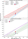 |
Fig. A.2. Total [OIII] luminosity as a function of SFR for the High-z model (red) and Schimek et al. (2024a,b) (purple). In the top panel we compare our models to observational data from Hashimoto et al. (2018) at z = 9, Harikane et al. (2020) at z ∼ 6, Hashimoto et al. (2019) at z ∼ 7, Inoue et al. (2016) at z ∼ 7, Witstok et al. (2022) at z = 6.7 − 7, Fujimoto et al. (2024) at z = 8.5, Algera et al. (2024) at z = 7.3, Laporte et al. (2017) at z = 8.3, Tamura et al. (2019) at z = 8.31, Ren et al. (2023) at z = 7.2, Carniani et al. (2017) at z ∼ 7, Popping (2023) (upper limit) at z = 13, and Schouws et al. (2025a,b) at z = 14.2. We used the relations from Harikane et al. (2020) for z = 6 − 9, as well as the SB and high-redshift relations from De Looze et al. (2014). In the bottom panel we compare our models to the simulated values from Katz et al. (2022) (z = 6), Pallottini et al. (2019) (z = 6), Lupi et al. (2020) (z = 6), Pallottini et al. (2022) (z = 7.7), and Ramos Padilla et al. (2023) (z = 6). The relations are from the simulations of Olsen et al. (2017) (z ≃ 6) and Arata et al. (2020) (z = 6 − 9). |
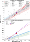
Appendix B: Dwarfs model and Halo model emission maps
In this section, we show the [CII] and [OIII] line emission maps and [OIII]/[CII] ratio maps obtained with the Dwarfs and Halo models. The [CII] maps are shown in Fig. B.1, with the Dwarfs model maps in the top panels and the Halo model maps in the bottom panels. The white dashed circles mark the virial radius of PONOS (Rvir = 21.18 kpc), and the right panels zoom in on the tidal tail between the merger B and merger A components. The Dwarfs model maps show a slightly weaker surface brightness in the disc and merger B component compared to the Solar model map, which reflects the overall lower (18%) total [CII] luminosity. The Halo model maps appear almost identical to the Solar model maps, which reflects the very small increase (3%) in total [CII] luminosity.
In Fig. B.2 we show the [OIII] emission maps obtained by the Dwarfs model (top panels) and Halo model (bottom panels), with the right panels zooming in on the tidal tail between the merger B and merger A components. The Dwarfs model maps are very similar to the High-z model maps, with stronger surface brightness in the CGM compared to the Solar model, reflecting the increased total [OIII] luminosity. The Halo model maps show a stronger surface brightness in the extended emission compared to the Solar model, where the total [OIII] luminosity obtained by the Halo model is the highest amongst our models.
Following the same method as for the Solar model and High-z model [OIII]/[CII] ratio maps (see Sect. 4.3), we show the [OIII]/[CII] ratio maps for the Dwarfs model (left panel) and the Halo model (right panel) in Fig. B.3. Both the Dwarfs model and Halo model maps reflect the models’ higher [OIII]/[CII] luminosity ratios compared to the Solar model.
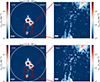 |
Fig. B.1. Emission maps of the [CII] line obtained with the Dwarfs model (top panels) and the Halo model (bottom panels). The right panels are zoomed-in images if the tidal tail between merger B and merger A. The dashed circles mark the extent of the virial radius of PONOS. |
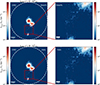 |
Fig. B.2. Emission maps of the [OIII] line obtained with the Dwarfs model (top panels) and the Halo model (bottom panels). The right panels are zoomed-in images of the tidal tail between merger B and merger A. The dashed circle marks the extent of the virial radius of PONOS. |
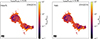 |
Fig. B.3. Ratio maps of the [OIII]/[CII] luminosity ratio, comparing the Dwarfs model (left) and the Halo model (right). The total luminosity ratios obtained with each model is shown in the title. |
All Tables
All Figures
|
Fig. 1. Gas surface density map of the PONOS simulation (left panel). The dashed circle corresponds to the virial radius, Rvir. The right panel shows the [C II] line surface density map obtained using the fiducial model of Schimek et al. (2024a,b), which assumes solar elemental abundances, zoomed into the galaxy disc and the merging companions. |
| In the text | |
|
Fig. 2. [C II] line emission maps obtained with the Solar model (top panels) and the High-z model (bottom panels). The right panels are zoomed-in images of the tidal tail between merger B and merger A. The white dashed circles mark the extent of Rvir of PONOS. The line emission maps obtained with the Dwarfs and Halo models are shown in Appendix B. |
| In the text | |
|
Fig. 3. [O III] line emission maps obtained with the Solar model (top panels) and the High-z model (bottom panels). The right panels are zoomed-in images of the tidal tail between merger B and merger A. The white dashed circles mark the extent of Rvir of PONOS. The line emission maps obtained with the Dwarfs and Halo models are shown in Appendix B. |
| In the text | |
|
Fig. 4. [N II] line emission maps obtained with the Solar model (top panels), the High-z model (middle panels), and the Dwarfs model (bottom panels). The right panels are zoomed-in images of the main disc and surrounding area. The white dashed circles mark the extent of Rvir of PONOS. |
| In the text | |
|
Fig. 5. Surface brightness ratio maps of the [O III]/[C II] luminosity ratio, comparing the Solar model (left panel) and the High-z model (right panel). The title above each panel gives the total luminosity ratios. The ratio maps obtained with the Dwarfs and Halo models are shown in Appendix B. |
| In the text | |
|
Fig. 6. Total [O III]/[C II] line luminosity ratio as a function of SFR for the High-z model (red) and Schimek et al. (2024a,b) (purple). The top panel reports the comparison with observational data from Hashimoto et al. (2019) at z ∼ 7, Witstok et al. (2022) at z = 6.7 − 7, Carniani et al. (2020) at z ∼ 6 − 9, missing [C II] flux corrected values from Carniani et al. (2020) (SBD corr.) at z ∼ 6 − 9, Harikane et al. (2020) at z ∼ 6, Ren et al. (2023) at z = 7.2, Algera et al. (2024) at z = 7.3, Bakx et al. (2020) at z = 8.31, Laporte et al. (2017) at z = 8.3, Fujimoto et al. (2024) at z = 8.5 (lower limit), and Schouws et al. (2025a,b) at z = 14.2 (lower limit). The relations included are the z = 6 − 9 relation from Harikane et al. (2020), the best-fit relation from Pallottini et al. (2022), and the high-redshift, local dwarfs, and local starbursts (SBs) relations from De Looze et al. (2014). The bottom panel reports the comparison with simulation studies by Katz et al. (2022) (z = 6), Ramos Padilla et al. (2023) (z = 6), Pallottini et al. (2022) (z = 7.7), and Lupi et al. (2020) (z = 6). The relations are from Arata et al. (2020) (z = 6 − 9) and Olsen et al. (2017) (z ≃ 6). |
| In the text | |
|
Fig. 7. [O III]/[C II] luminosity ratio vs. metallicity Z/Z⊙ in PONOS. Our models are colour-coded based on the assumed C/O abundance ratios. The circle symbols correspond to the luminosity ratios and average metallicities computed for the whole simulated halo (log(Z/Z⊙) = − 0.55). The diamonds show the contribution from the main disc and merger B component only (log(Z/Z⊙) = − 0.22). The grey dashed line is the best-fit relation from Arata et al. (2020) for their simulated sample of z = 6 − 9 galaxies, with the grey area corresponding to their ≲0.2 dex dispersion. The grey symbols are the PONOS models shifted to the metallicity values expected from the Arata et al. (2020) relation. |
| In the text | |
|
Fig. 8. Total [N II] luminosity (top panel) and [N III] luminosity (bottom panel) as functions of SFR for the High-z model (red), Dwarfs model (orange), and Schimek et al. (2024a,b) (purple). Both panels include comparisons with the simulated z = 6 sample from Ramos Padilla et al. (2023) (grey circles) and the linear relations from Mordini et al. (2021) based on observations of galaxies in the local Universe. In the top panel we include the [N II] observation from Killi et al. (2023) (black circle) at z ∼ 7, the observed upper limits from Harikane et al. (2020) at z ∼ 6 and Sugahara et al. (2021) at z ∼ 7 (black circles with arrows), and the theoretical relation from Kannan et al. (2022) (z = 6 − 10). |
| In the text | |
|
Fig. 9. [O III]/[N II] as a function of metallicity Z [Z⊙] for the Solar model (yellow-green), High-z model (red) and Dwarfs model (orange). The circles show the contribution from the whole galactic halo, while the diamonds consider only the main disc and merger B. The shaded regions are the model predictions of the [O III]/[N II] ratio as functions of metallicity from Pereira-Santaella et al. (2017), with each shaded region corresponding to a model assuming a certain ionisation parameter: log(U) = − 4, −3.5, −3, −2.5 and −2. The width of the shaded regions spans the density range: log(nH) = 1 − 4. The grey star represents the observed ratio from Killi et al. (2023) at z ∼ 7. |
| In the text | |
|
Fig. A.2. Total [OIII] luminosity as a function of SFR for the High-z model (red) and Schimek et al. (2024a,b) (purple). In the top panel we compare our models to observational data from Hashimoto et al. (2018) at z = 9, Harikane et al. (2020) at z ∼ 6, Hashimoto et al. (2019) at z ∼ 7, Inoue et al. (2016) at z ∼ 7, Witstok et al. (2022) at z = 6.7 − 7, Fujimoto et al. (2024) at z = 8.5, Algera et al. (2024) at z = 7.3, Laporte et al. (2017) at z = 8.3, Tamura et al. (2019) at z = 8.31, Ren et al. (2023) at z = 7.2, Carniani et al. (2017) at z ∼ 7, Popping (2023) (upper limit) at z = 13, and Schouws et al. (2025a,b) at z = 14.2. We used the relations from Harikane et al. (2020) for z = 6 − 9, as well as the SB and high-redshift relations from De Looze et al. (2014). In the bottom panel we compare our models to the simulated values from Katz et al. (2022) (z = 6), Pallottini et al. (2019) (z = 6), Lupi et al. (2020) (z = 6), Pallottini et al. (2022) (z = 7.7), and Ramos Padilla et al. (2023) (z = 6). The relations are from the simulations of Olsen et al. (2017) (z ≃ 6) and Arata et al. (2020) (z = 6 − 9). |
| In the text | |
|
Fig. B.1. Emission maps of the [CII] line obtained with the Dwarfs model (top panels) and the Halo model (bottom panels). The right panels are zoomed-in images if the tidal tail between merger B and merger A. The dashed circles mark the extent of the virial radius of PONOS. |
| In the text | |
|
Fig. B.2. Emission maps of the [OIII] line obtained with the Dwarfs model (top panels) and the Halo model (bottom panels). The right panels are zoomed-in images of the tidal tail between merger B and merger A. The dashed circle marks the extent of the virial radius of PONOS. |
| In the text | |
|
Fig. B.3. Ratio maps of the [OIII]/[CII] luminosity ratio, comparing the Dwarfs model (left) and the Halo model (right). The total luminosity ratios obtained with each model is shown in the title. |
| In the text | |
Current usage metrics show cumulative count of Article Views (full-text article views including HTML views, PDF and ePub downloads, according to the available data) and Abstracts Views on Vision4Press platform.
Data correspond to usage on the plateform after 2015. The current usage metrics is available 48-96 hours after online publication and is updated daily on week days.
Initial download of the metrics may take a while.