| Issue |
A&A
Volume 702, October 2025
|
|
|---|---|---|
| Article Number | A177 | |
| Number of page(s) | 17 | |
| Section | Extragalactic astronomy | |
| DOI | https://doi.org/10.1051/0004-6361/202453412 | |
| Published online | 17 October 2025 | |
CASCO: Cosmological and AStrophysical parameters from Cosmological simulations and Observations
III. The physics behind the emergence of the golden mass scale
1
INAF – Osservatorio Astronomico di Capodimonte, Salita Moiariello 16, I-80131
Napoli, Italy
2
Dipartimento di Fisica “E. Pancini”, Università degli studi di Napoli Federico II, Compl. Univ. di Monte S. Angelo, Via Cintia, I-80126
Napoli, Italy
3
INFN, Sez. di Napoli, Compl. Univ. di Monte S. Angelo, Via Cintia, I-80126
Napoli, Italy
4
Kapteyn Astronomical Institute, University of Groningen, P.O. Box 800
9700 AV
Groningen, The Netherlands
5
Center for Computational Astrophysics, Flatiron Institute, 162 5th Avenue, New York, NY, 10010
USA
6
Columbia Astrophysics Laboratory, Columbia University, 550 West 120th Street, New York, NY, 10027
USA
7
Department of Astrophysical Sciences, Princeton University, 4 Ivy Lane, Princeton, NJ, 08544
USA
⋆ Corresponding author: This email address is being protected from spambots. You need JavaScript enabled to view it.
Received:
12
December
2024
Accepted:
10
July
2025
Abstract
Observations reveal a characteristic ‘golden mass’ (around 1012 M⊙ in halo mass and 5 × 10¹⁰ M⊙ in stellar mass) associated with a peak in star formation efficiency. Using the CAMELS simulations based on IllustrisTNG in a (50 h−1 Mpc)3 volume, we investigate how this scale arises and evolves under varying supernova (SN) and active galactic nucleus (AGN) feedback strengths and cosmological parameters (Ωm, σ8). We find a U-shaped relation between the dark-to-stellar mass ratio (within the half-mass radius) and stellar mass, with a minimum at the golden mass, in line with observations. Cosmology primarily shifts the normalization of the scaling relation, while SN and AGN feedback modify both the shape and the emergence of the golden mass. Stronger SN feedback shifts the golden mass to lower values, while AGN feedback–especially the radiative efficiency (i.e. the fraction of the accretion rest mass released in the accretion process), followed by the black hole feedback factor (i.e. the normalization factor for the energy in the AGN feedback in the high-accretion state) and the quasar threshold (i.e. the Eddington ratio)–affects the high-mass slope and shifts the golden mass value. The golden mass appears earlier in cosmic time for simulations with stronger feedback, which more rapidly quenches star formation in massive galaxies. Splitting galaxies by star formation activity reveals that passive galaxies preserve the U-shape, while star-forming galaxies show a decreasing dark matter fraction with stellar mass, with hints of a reversal at low redshift. Global stellar fractions also follow a U-shaped trend. However, in passive systems, the golden mass disappears, shifting to lower masses, while star-forming galaxies exhibit a peak only at low redshift. Our results highlight feedback as the primary driver behind the emergence of the golden mass up to z ∼ 1.5 − 2, while stream and virial shock processes play a secondary role. Comparing our results with other theoretical expectations and observational findings, we speculate that at z ≳ 1.5 − 2, a single characteristic (stream) mass regulates galaxy evolution, which later bifurcates into two: a low-mass gas-richness scale tied to gas availability, and a higher-mass golden mass governing star formation efficiency and quenching.
Key words: methods: numerical / galaxies: evolution / galaxies: formation / dark matter
© ESO 2018
 Open Access article, published by EDP Sciences, under the terms of the Creative Commons Attribution License (http://creativecommons.org/licenses/by/4.0), which permits unrestricted use, distribution, and reproduction in any medium, provided the original work is properly cited.
1. Introduction
Research using spectroscopic and photometric data have led to the characterization of scaling relations among various galaxy parameters, including stellar populations (age, metallicity, luminosity, stellar mass, IMF slope), structural properties (e.g. galaxy size and light profile), and total mass and dark matter (DM) distributions (DM fraction, mass density slope). Understanding the origins of these scaling relations, the physical processes shaping them, and their role in galaxy evolution across a vast range of masses and cosmic time is central to modern studies of galaxy evolution (e.g. Courteau et al. 2014; D’Onofrio et al. 2021).
There is growing evidence that a critical stellar mass scale exists around ∼5 × 10¹⁰ M⊙, corresponding to ∼1012 M⊙ in virial mass (e.g. Dekel & Birnboim 2006). This characteristic mass, often referred to as the golden mass, the transition mass, or the bimodality mass, appears as a transition, break, or extremum in the trends of various scaling relations. Given the power-law nature of the DM power spectrum from simulations (Widrow et al. 2009), there is no reason to consider any particular mass scale as special. In contrast, the stellar mass function follows a Schechter form. As a result, near the break of the stellar mass function, star formation efficiency, i.e. the ratio of stellar to halo mass normalized by the cosmological baryon fraction (ϵSF = M⋆/(Mhfb)), reaches its peak, whereas at both higher- and lower-mass scales, feedback mechanisms reduce this efficiency. Thus, any characteristic mass scale is likely tied to baryonic processes rather than DM dynamics.
If this is indeed a fundamental mass scale in galaxy formation and evolution, it is plausible that the physical processes driving galaxy evolution also change when crossing this mass threshold. One well-studied scaling relation involves total virial mass and stellar mass, which can be translated into a relation between the star formation efficiency and stellar or virial mass (e.g. Moster et al. 2010). The bending observed in the virial-to-stellar mass relation translates into a peak in the correlation between stellar fraction (or star formation efficiency) and mass at the golden mass. Analysing the correlation between stellar fraction or star formation efficiency with mass can provide insights into the role of various galactic processes, for example SN and AGN feedback, which are believed to dominate at low and high masses, respectively. At the golden mass, supernova-driven winds and AGN feedback become less effective at depleting the galaxy’s gas supply and quenching star formation (e.g. Dekel & Birnboim 2006; Moster et al. 2010). Moreover, Dekel & Birnboim (2006) have proposed that one of the primary drivers of the bimodality in galaxy properties is the transition from cold gas inflows to virial shock heating at a critical virial mass scale of ∼ 1012 M⊙, in conjunction with cold streams at high redshifts, feedback processes, and gravitational clustering (Daddi et al. 2022a,b).
The dark matter fraction within the half-light radius in early-type systems exhibits a U-shaped trend (Tortora et al. 2016, 2019), the inverse counterpart of the bell-shaped behaviour of star formation efficiency on a global scale. However, tensions arise when considering different galaxy types. A bending in the trend of star formation efficiency with mass is not seen in recent analyses of rotation curves of star-forming galaxies (SFGs, Posti et al. 2019). Using the same data as in Posti et al. (2019), Tortora et al. (2019) only found some mild evidence of bending in such scaling relations.
Understanding the nature of the golden mass is therefore a central question to unravelling the physical processes governing galaxy formation. Despite the progress, the physics underlying these scaling relations remains unclear, and leaves key questions regarding the processes that shape the observed scaling relations and their extent, why the golden mass emerges and how it manifests, and whether this golden mass is constant in time or if it shows up at some specific epoch as a consequence of a dominating physical mechanism governing its appearance. We are also looking into how these relations and the golden mass vary with galaxy types and whether different extrema and bends in scaling relations all measure the same mass scale. In particular, it would be interesting to analyse whether feedback, virial shocks, and cold streams act independently, are interconnected, or if one plays a more dominant role than the others in explaining the golden mass. All these questions can be addressed by exploring the predictions of cosmological simulations and comparing them with observations (e.g. Mukherjee et al. 2018, 2021, 2022 Busillo et al. 2023, 2025).
We began exploring these issues in the first two papers of the Cosmological and AStrophysical parameters from Cosmological simulations and Observations (CASCO) series, using CAMELS simulations within a volume of (25 h−1 Mpc)3, one of the most advanced suites of cosmological simulations, which allows for variation in cosmological parameter values and, more relevantly for this paper, the strength of SN and AGN feedback (Villaescusa-Navarro et al. 2021, 2023; Ni et al. 2023). By identifying the best simulations that reproduce different observed scaling relations among central DM mass and fraction, total virial mass, and half-mass radius versus stellar mass for different data samples (for both passive and star-forming galaxies) in Busillo et al. (2023, Paper I hereafter) and Busillo et al. (2025, Paper II hereafter), we have constrained cosmological and astrophysical parameters.
In this third paper in the CASCO series, we address the aforementioned open questions from a theoretical point of view, focusing on the origin of the golden mass. We use the latest CAMELS simulations, which improve the galaxy count statistics by increasing the simulation volume eightfold to (50 h−1 Mpc)3. We examine the scaling relations between the DM-to-stellar mass ratio within the half-mass radius and stellar mass, as well as the correlation between half-mass radius and stellar mass, and total stellar mass fraction and stellar mass, as a function of redshift to decipher the impact of SN and AGN feedback.
The paper is organized as follows. We start by providing a summary of the observational and simulation findings on the golden mass in Sect. 2. In Sect. 3 we present the simulations. The results on the effect of astrophysical and cosmological parameters on the scaling relations and the golden mass are discussed in Sect. 4. The results are discussed in a broader context and compared with the literature in Sect. 5 and a summary of paper findings with future prospects is provided in Sect. 6.
2. The state of the art of the golden mass
2.1. Characteristic mass scales in galaxy evolution
Across the galaxy mass spectrum characteristic transition masses in galaxy properties exist. In particular, Kannappan et al. (2013) has identified two characteristic mass scales in galaxy morphology, gas fractions, and fueling regimes (see also Hunt et al. 2020), which separate three regimes: ‘accretion-dominated’ dwarf galaxies, ‘gas-equilibrium’ or ‘processing-dominated’ intermediate-mass galaxies, and ‘gas-poor’ or ‘quenched’ massive galaxies. Below a stellar mass threshold of ∼ 3 × 10⁹ M⊙ dwarf galaxies are characterized by an overwhelming gas accretion, this mass scale can appear as a break in the HI-mass vs stellar mass relation (Hunt et al. 2020). The mass scale of ∼ 3 × 10⁹ M⊙ is termed ‘gas-richness’ threshold. Above this mass we enter into a processing-dominated regime, where such intermediate-mass galaxies are able to consume gas through star formation as fast as it is accreted. This regime ends up at a mass threshold of ∼ 3 × 10¹⁰ M⊙, the bimodality or golden mass. Above this mass scale, we have a gas-poor or quenched regime, populated by spheroid-dominated gas-poor galaxies with low rates of star formation over the last billion year.
2.2. The golden mass from observations
The golden mass is observed in several contexts, including the trends of total mass-to-light ratio and halo mass with stellar mass (e.g. Benson et al. 2000; Marinoni & Hudson 2002; van den Bosch et al. 2007; Conroy & Wechsler 2009; Moster et al. 2010, 2013; Behroozi et al. 2013; Rodríguez-Puebla et al. 2015; Behroozi et al. 2019; Girelli et al. 2020). The stellar-to-halo mass relation (SHMR), or equivalently the star formation efficiency–mass relation, has been extensively studied in recent years, both in cumulative form and by separating galaxy samples by type. The bending in the SHMR translates into a peak in the trend between star formation efficiency and mass. This value is Mh ∼ 1012 M⊙ when DM halo masses are considered, corresponding to a stellar mass value of ∼ 3 × 10¹⁰ M⊙.
It also manifests in the half-light dynamical M/L and DM fraction (Wolf et al. 2010; Toloba et al. 2011; Cappellari et al. 2013; Tortora et al. 2016, 2019; Aquino-Ortíz et al. 2018; Lovell et al. 2018; Busillo et al. 2023, 2025), in the gradients of dynamical M/L profiles across several effective radii (Napolitano et al. 2005), and in the total mass density slope of galaxies (Tortora et al. 2019). Historically, this mass scale has emerged from structural analyses, such as the correlation between effective surface brightness and effective radius (Capaccioli et al. 1992, Tully & Verheijen 1997, Kormendy et al. 2009) and size-mass relations (Shen et al. 2003; Hyde & Bernardi 2009; Tortora et al. 2009; Nedkova et al. 2021), as well as in trends of optical colour, metallicity, and stellar M/L gradients (Kuntschner et al. 2010; Spolaor et al. 2010; Tortora et al. 2010, 2011). Different works also find a bending in the main sequence of star-forming galaxies, which is associated with the golden mass (Daddi et al. 2022a; Popesso et al. 2023; Stephenson et al. 2024; Euclid Collaboration: Enia et al. 2025). This extensive body of empirical evidence mostly converges on a value for the golden stellar mass around 1 − 5 × 10¹⁰ M⊙ at z ∼ 0.
Tensions arise when the SHMR is analysed considering different galaxy types (e.g. Dutton et al. 2010; More et al. 2011; Wojtak & Mamon 2013; Posti et al. 2019; Correa & Schaye 2020). A bending in the SHMR is not seen in the analyses of rotation curves of star-forming galaxies by Posti et al. (2019), pointing to larger star formation efficiencies of late-type systems when compared to early types of similar stellar mass above the golden mass. Building SHMRs through statistical approaches that combine various semi-empirical methods of galaxy–halo connection, Rodríguez-Puebla et al. (2015) found a segregation in colour for central galaxies, with bluer galaxies having a larger stellar fraction than red galaxies at fixed virial mass. Using SDSS data with visual classifications, Correa & Schaye (2020) found that disks have stellar masses (and hence star formation efficiencies) that are larger or equal to those of ellipticals at virial masses below 1013 M⊙, and less massive at larger virial masses; EAGLE simulations also indicate that disks are more massive than ellipticals at fixed virial mass. In contrast to Posti et al. (2019), both studies observed the golden mass in both galaxy types. When the same quantities are calculated in the central galactic regions and transformed into a DM fraction within the half-light radius, early-type galaxies exhibit a U-shaped trend (Tortora et al. 2016, 2019). Using the same data as in Posti et al. (2019), Tortora et al. (2019) only found some mild evidence of a bending in such scaling relations for late-type galaxies.
Some analysis, mostly concerning the SHMR and the main sequence of star-forming galaxies have probed bendings as a function of redshift. Behroozi et al. (2013) shows that the instantaneous star formation efficiency peaks at Mh ∼ 1011.7 M⊙ at z ∼ 0, and varies very little since z = 4. Modelling the main sequence of star-forming galaxies, using a power law with a turnover mass, Popesso et al. (2023) find a value, in stellar mass, of ∼ 1010 M⊙ at low redshifts, which increases to ∼ 1011 M⊙ at z ∼ 6. Translated to halo masses, these authors find a mass of ∼ 1011.4−11.5 M⊙ at z ∼ 0, with a steep increase at z ≳ 0.8, up to ∼ 1013 M⊙ at z ∼ 6 (see also Lee et al. 2015; Delvecchio et al. 2021; Daddi et al. 2022a; Euclid Collaboration: Enia et al. 2025). Analysing the size-mass relation as a function of redshift, Nedkova et al. (2021) find a monotonic trend in star-forming galaxies, while the relation is steeper for quiescent galaxies with stellar masses above ∼ 1010.3 M⊙ and flattens at lower masses. From their Figure 10 we observe that the bending mass for passive galaxies is increasing with redshift.
2.3. Theoretical interpretation of the golden mass
If historically SN and AGN feedback have been supposed to be the leading processes in galaxies evolution, with a varying role as a function of mass, more recently the role of the virial shock heating and cold streams have emerged as alternative or complementary processes. The interplay of such processes is supposed to influence the emergence of the golden mass.
In galaxies with stellar masses below the golden mass, SN feedback plays a crucial role in regulating star formation. The energy released by supernova explosions can heat the surrounding circum-galactic medium (CGM) and, in some cases, expel gas from the galaxy. This process is particularly effective in low-mass galaxies, where the gravitational potential wells are shallower, making it easier for the gas to escape. The effectiveness of SN feedback decreases with increasing galaxy mass, as the deeper gravitational potentials in more massive galaxies can better retain the heated gas. Using the theory of supernova bubble in Dekel & Silk (1986), equating the energy released in the interstellar medium to the binding energy of this gas in the DM halo potential well, gives an upper limit for the mass of a halo in which SN feedback can be effective of MSN ∼ 1011.7 M⊙ at z ∼ 0, scaling with redshift as (1 + z)−3/2 (Dekel & Birnboim 2006).
At low masses, SN feedback suppresses the supermassive black holes (SMBHs) growth. In more massive halos, the deep gravitational potential and hot CGM confine the central gas, enabling sustained accretion onto the black hole (Dubois et al. 2015; Bower et al. 2017; Habouzit et al. 2019). Therefore, above a critical mass scale the growth of SMBHs at the centres of galaxies becomes more pronounced. The energy and momentum output from AGN can drive powerful outflows, heating and expelling gas from the galaxy and its surrounding CGM. This AGN feedback further suppresses star formation by depleting the cold gas reservoir necessary for star formation and maintaining the hot state of the CGM. The onset of significant AGN activity around the golden mass is also associated with morphological transformations in galaxies, such as the transition from disk-like to spheroidal structures. From these considerations the maximum mass for effective SN feedback emerge as a lower limit for impactful AGN feedback (MAGN ∼ MSN).
Virial shock heating and cold streams are competing, complementary or supporting processes (Dekel & Birnboim 2006; Dekel et al. 2019; Stern et al. 2020; Aung et al. 2024; Waterval et al. 2025). Hydrodynamical simulations predict that for low halo masses gas accretes in cold filaments (‘cold-mode accretion’) directly to the galaxy disk, efficiently forming stars. However, as galaxies grow in mass, they reach a point where the infalling gas is shock-heated to the virial temperature of the DM halo (‘hot-mode accretion’) and star formation is rapidly quenched. This virial shock heating becomes significant in halos with masses around Mshock ∼ 1011.7 M⊙ (which is predicted to be redshift-independent for z < 3), which approximately corresponds to the mass where SN and AGN feedback efficiency is minimal. The shock-heated gas forms a hot, diffuse CGM that is less prone to cooling and condensing into the galaxy, thereby suppressing further star formation. This mechanism is supposed to contribute to the decline in star formation efficiency observed in more massive galaxies. However, at z ≳ 1.5, narrow cold streams are expected to penetrate the otherwise hot CGM and sustain efficient star formation, even in halos exceeding the critical mass for shock heating (e.g. Kereš et al. 2005).
Recent works show that the bending in the star-forming main sequence across redshift can be connected to virial shocks and cold streams (Daddi et al. 2022a; Popesso et al. 2023; Stephenson et al. 2024). In particular, when converting turnover mass in the main sequence of star-forming galaxies into hosting DM halo masses, Daddi et al. (2022a) find consistent results with the evolving cold- to hot-accretion transition mass, defined by the redshift-independent Mshock at z < 1.4 and by the rising Mstream at z > 1.4.
Given the considerations above, several key aspects remain unexplored. It is still unclear whether feedback processes, virial shocks, and the physics of the CGM represent competing scenarios, or whether they offer independent or interconnected explanations for the origin of the golden mass. The CAMELS cosmological simulations can help disentangle these effects by assessing the impact of feedback mechanisms and quantifying the role of virial shocks when feedback is suppressed.
Although less explored in the literature, we centre our analysis on the relationship between central DM content and stellar mass. These are measurable quantities that are expected to become increasingly accessible in the near future through dynamics using spectroscopic surveys (de Jong 2011; Iovino et al. 2023a,b) and strong lensing (Euclid Collaboration: Walmsley et al. 2025). Our goal is to derive theoretical expectations for the golden mass based on this correlation and compare them with independent observational findings.
3. Data
Following Papers I and II, we use the simulated galaxy data coming from CAMELS, a suite of cosmological simulations, originally within a cosmological volume of (25 h−1 Mpc)3 (Villaescusa-Navarro et al. 2021, 2023; Ni et al. 2023). In this paper, we also use a new suite of simulations, where the Universe volume is increased by eight times to (50 h−1 Mpc)3. The specific details of the simulations, other than the volume, are already described in detail in Paper I and II. Each simulation has the following cosmological parameter values fixed: Ωb = 0.049, ns = 0.9624 and h = 0.6711. We limit the data to the CAMELS simulations based on the IllustrisTNG subgrid physics. The masses and radii of the galaxies investigated in this paper significantly exceed particle mass resolutions and softening length, respectively.
The fiducial CAMELS simulation uses the same parameters of IllustrisTNG, which is calibrated to observations. These calibrations have been performed by using the galaxy stellar mass function, the stellar-to-halo mass relation, the total gas mass content within the virial radius r500 of massive groups, the stellar size – stellar mass and the black hole (BH) mass – galaxy mass relations, all at z = 0, and, finally, the functional shape of the cosmic star formation rate density for z ≲ 10 (Pillepich et al. 2018).
With respect to the original CAMELS suites, which allowed for the variation of only six parameters, the updated set of simulations allows us to explore the role of 28 astrophysical and cosmological parameters in total. In particular, we vary the two cosmological parameters (Ωm, σ8), the originally implemented SN- and AGN-feedback parameters (ASN1, ASN2, AAGN1, and AAGN2) and six more parameters regulating AGN feedback. In particular, ASN1 and ASN2 are related to the SN feedback mechanisms, wind energy and velocity, respectively. Instead, AAGN1 and AAGN2 are the normalization factors of energy and frequency of AGN feedback (Villaescusa-Navarro et al. 2021). However, previous papers have demonstrated that AAGN1 and AAGN2 have no effect on scaling relations (see for example Papers I and II), and therefore we only investigate the impact of the six other AGN feedback parameters, which have been implemented in the latest CAMELS release. The complete list of parameters we consider in this paper are listed in Table 1. We use the ‘1P’ simulations, where we can vary one of the parameters at a time, holding the rest of the parameters constant (e.g. Villaescusa-Navarro et al. 2021). The values of the simulation parameters varied in each ‘1P’ simulation set (including the fiducial simulation ones) are listed in Table 2. In the rest of the paper, astrophysical parameter values are normalized to the parameter value of the fiducial simulation, which corresponds to the unit value in our figures.
Free parameters of CAMELS simulations used in this paper (for more details, see Ni et al. 2023).
Differently from our previous papers, where we analysed different scaling relations, comparing simulations with observations, in the present paper we only use the simulations and mostly the scaling relation MDM, 1/2/M⋆, 1/2 vs. M⋆ where MDM, 1/2 and M⋆, 1/2 are the 3D DM and stellar mass calculated within the 3D stellar half-mass radius, respectively, M⋆ is the total stellar mass1, and Mtot is the total mass. For completeness, and for connecting the central galaxy regions to the whole galaxy, we also investigate the correlation between the total M⋆/MDM and stellar mass. We explore how these scaling relations are varying as a function of redshift, using simulations at the following redshift slices: 0, 0.5, 1.0, 1.5 and 2.
Similarly to the previous work, we performed a filtering of the subhalos detected by SUBFIND. We considered only subhalos that have R⋆, 1/2 > ϵmin, N⋆, 1/2 > 50 and fDM(< R⋆, 1/2)≡1 − M⋆, 1/2/Mtot, 1/2 > 0, where ϵmin = 2 ckpc is the gravitational softening length of the IllustrisTNG suite2. The selection criteria on R⋆, 1/2 and N⋆, 1/2 prevent strong resolution biases.
Similarly to Paper I and II, we follow Bisigello et al. (2020) for the selection of passive galaxies (PGs) and SFGs via specific SFR (sSFR := SFR/M⋆), choosing for the PGs only subhalos having log10(sSFR/yr−1) < −10.5, and the opposite for SFGs. We have verified that varying the sSFR threshold by ±0.5 dex does not affect our results (see Paper I)3. Although not a central focus of this paper, we also investigate the SFG main sequence and compare it with results from the literature in Appendix A.
The key observables from the simulations used in this paper are listed in Table 3.
Observables used in the paper.
4. The golden mass
Using the same parameters of the reference IllustrisTNG, calibrated, among other factors, to the observed z = 0 size-stellar mass and halo-to-stellar mass relations, the fiducial CAMELS simulation reveals a bending in the simulated size-stellar mass and halo-to-stellar mass relations around a mass of approximately 5 × 10¹⁰ M⊙ (see also Paper I and II). This mass scale is transferred, for example, into the correlation among MDM, 1/2/M⋆, 1/2 and M⋆ and any other related scaling relation. Therefore this feature and the specific shape of these observed scaling relations are naturally and by construction introduced during the calibration of the reference simulation. However, since this calibration is not transferred to the other simulations with varied parameters, the scaling relations are no longer primarily influenced by the initial calibration. While the calibration process prevents a fully agnostic analysis of the emergence of the golden mass scale, it firmly enables us to assess the impact of cosmology and astrophysical processes on the shape of the scaling relations, as well as the emergence and value of the golden mass over cosmic time.
One significant limitation of the CAMELS simulations is the relatively small cosmological volume, which restricts the number of massive objects, especially in the mass range where the golden mass is expected to appear. However, compared to the original CAMELS simulations, which simulate a volume of (25 h−1 Mpc)3, the current suite increases the volume, resulting in a galaxy count eight times larger. This increase in sample size is particularly important in the high-mass range (M⋆ > 5 × 10¹⁰ M⊙), where galaxies are less abundant, as it facilitates the determination of the golden mass.
To estimate the golden mass as a function of the simulation parameters, for each simulation we fit a parabola to the simulation data in the vicinity of the minimum in the scaling relation. The results for the z = 0 snapshot are summarized in Table 44. The typical uncertainty in the (log) golden mass is approximately 0.1 − 0.2 dex.
Golden mass estimates in log M⋆/M⊙, at z = 0.
4.1. Golden stellar mass
We investigate the impact of the twelve simulation parameters listed in Table 1 on the MDM, 1/2/M⋆, 1/2–M⋆ scaling relation in Figs. 1, 2 and 3. Following the results presented in Paper II, for most of the simulations a U-shaped curve, with a minimum at the golden stellar mass, is observed. In particular, for the reference simulation, it takes the value of ∼ 5 × 10¹⁰ M⊙. This result confirms what has been found combining observations for dwarf and giant early types and late types (Tortora et al. 2016, 2019) and not surprisingly results from Illustris TNG (Lovell et al. 2018).
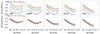 |
Fig. 1. MDM, 1/2/M⋆, 1/2 plotted against M⋆ for the CAMELS simulations. Each row shows variations in the cosmological parameters Ωm and σ8. The green lines represent the reference CAMELS simulation. To examine the evolution across redshift, simulation snapshots at z = 0, z = 0.5, z = 1, z = 1.5, and z = 2 are displayed from left to right. The medians in stellar mass bins are shown. For the reference simulation the 16-84th percentile range is also shown as a shaded green region. |
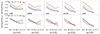 |
Fig. 2. MDM, 1/2/M⋆, 1/2 plotted against M⋆ for the CAMELS simulations. Each row shows variations in the SN-related parameters ASN1 and ASN2. The green lines represent the reference CAMELS simulation. To examine the evolution across redshift, simulation snapshots at z = 0, z = 0.5, z = 1, z = 1.5, and z = 2 are displayed from left to right. The medians in stellar mass bins are shown. |
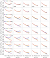 |
Fig. 3. MDM, 1/2/M⋆, 1/2 plotted against M⋆. Each row shows variations in the AGN-related simulation parameters: AAGN1, AAGN2, BHaccr, BHEdd, BHFF, BHRE, QT, and QTP from top to bottom. The green lines represent the reference CAMELS simulation. To examine the evolution across redshift, simulation snapshots at z = 0, z = 0.5, z = 1, z = 1.5, and z = 2 are displayed from left to right. The medians in stellar mass bins are shown. |
4.1.1. Cosmological parameters
In Fig. 1, where only the cosmological parameters are varied, and the rest of parameters are fixed to the values of the fiducial simulations, we show that the impact of Ωm on the scaling relation is more significant than that of σ8 (reconfirming the findings reported in Papers I and II). Higher values of both parameters result in galaxies with greater DM content, although their impact on the golden mass appears negligible. We observe only a very mild flattening at the high-mass end for the largest σ8 values. In general, we observe that the minimum in the scaling relation begins to emerge between z = 1.5 and z = 1, becoming definitively established around z = 0.5.
4.1.2. SN feedback parameters
In Fig. 2 we show the impact of SN feedback, by limiting the analysis to the two parameters ASN1 and ASN2, which determine the amplitude of the SN wind energy per unit star formation rate and the wind velocity, respectively. These are among the most influential parameters.
Consistent with findings in Papers I and II, we confirm that the SN energy per unit SFR parameter (ASN1) is one of the most significant astrophysical parameters affecting our scaling relation (Paper I). Specifically, stronger wind energy corresponds to higher values of MDM, 1/2/M⋆, 1/2 at a fixed stellar mass. We can now also quantify the effect on the golden mass scale and the steepness of the scaling relation at masses below and above this scale. Notably, for low wind energy values, the bending is mild, and the golden mass becomes more pronounced as this parameter increases, becoming particularly well-defined for very strong wind energy. While the slope of the correlation at masses below the golden mass remains almost constant, the correlation for massive galaxies – dominated by PGs – becomes increasingly steeper as a function of wind energy. In the simulation with the strongest wind energy (ASN1 = 4), the minimum–and thus the golden mass–occurs at z ∼ 1.5. In contrast, simulations with weaker wind energy show that the minimum occurs at lower redshifts, with most models only revealing it at z ∼ 0. In particular, at z = 0, we observe a decrease in the golden mass as ASN1 increases, dropping from 7 × 10¹⁰ M⊙ to 3 × 10¹⁰ M⊙.
The impact of the wind velocity amplitude, ASN2, is more complex. At a fixed mass, as discussed in Paper II, the trend at high mass is similar to that of ASN1, with larger values corresponding to higher DM content. However, the trend is reversed at lower masses, where LTGs dominate. Regarding the emergence of the golden mass, similar to ASN1, the bending in the scaling relation is almost absent for the lowest wind velocity values, with the golden mass appearing at around 1011 M⊙. The bending becomes stronger with increasing wind velocity. A stronger decrease in the golden mass value is observed with increasing ASN2, ranging from approximately 1011 to ∼ 3 × 10¹⁰ M⊙ for the extreme values of the parameter. When studying the correlations as a function of redshift, we find that a bend in the model with the highest wind velocity (ASN2 = 2) is already present at z = 2, but the minimum in the relation only emerges at z = 1. In most models with lower ASN2 values, the golden mass appears at z ≲ 0.5.
4.1.3. AGN feedback parameters
The impact of eight parameters which regulate the AGN feedback in CAMELS simulations are finally investigated in Fig. 3.
As noted in our previous papers (see also Villaescusa-Navarro et al. 2023 and Chawak et al. 2023), the normalization factors for the energy and the frequency of events, i.e. AAGN1 and AAGN2, have a negligible effect on scaling relations, which we confirm for both the normalization of these relations and their impact on the golden mass scale. We only observe a minor effect on the slope of the trend in massive galaxies varying AAGN1 at z < 0.5.
In contrast, the impact of other AGN feedback parameters on the scaling relation is more significant, as it is expected to happen in the most massive galaxies, hosting super-massive BHs.
Larger values of the BH accretion factor BHaccr, BH Eddington factor BHEdd, quasar threshold QT, and quasar threshold power QTP result in higher DM fractions at larger masses and introduce a bend in the scaling relation. For most of these parameters, and in simulations with their highest values, the golden mass is established around z ∼ 1. For lower values of these parameters, the golden mass emerges at later redshifts. For BH accretion factor, quasar threshold, and quasar threshold power, larger golden mass values correspond to smaller parameter values. Focusing on the z = 0 snapshot, smaller values of BHaccr, i.e. smaller values for the normalization factor of the Bondi rate, push the golden mass to ∼ 1011 M⊙, while it remains nearly stable for values greater than or equal to the fiducial. For BHEdd, models that show a clear minimum are those with values ≥ the fiducial, above which the golden mass stabilizes; therefore the normalization factor for the limiting Eddington rate is not impacting the golden mass value. QT regulates the threshold between the AGN feedback low- and high-accretion states, and is one of the parameters with the greatest impact on the golden mass, reducing it from 1011 M⊙ in the weaker models to 3 × 10¹⁰ M⊙ in the strongest models. Finally, the power-law index of the scaling relation of the low- to high-accretion state threshold with BH mass, i.e. the quasar threshold power (QTP), shows a bending trend starting from QTP = 0.5, with the golden mass and trends saturating for values ≥ the fiducial simulation.
The opposite trend is observed for the BH feedback factor BHFF, i.e. the normalization factor for the energy in AGN feedback in the high-accretion state, and the BH radiative efficiency BHRE, corresponding to the fraction of accretion rest mass released in the accretion process. In these cases, larger parameter values correspond to smaller DM fractions compared to lower values. For the smallest values of BHRE, the golden mass is already established at z ∼ 2, while for larger values, it never appears. Regarding the BH feedback factor, the golden mass emerges across all models at z < 1. For both parameters, larger golden mass values correspond to larger parameter values. At z = 0, although the BH feedback factor BHFF has a greater impact on DM normalization, the golden mass saturates at the lower end of the parameter range, increasing beyond the fiducial model up to ∼ 1011 M⊙ for the highest parameter values. Finally, the fraction of accretion rest mass that is released in the accretion process proves to be the most influential parameter. Indeed, for the weakest values of BHRE, the golden mass is approximately 2 × 10¹⁰ M⊙, whereas for the largest values, it exceeds 1011 M⊙.
4.1.4. The connection with the size-mass relation
We have seen that the golden mass is well defined and appears in earlier cosmic times in simulations with a stronger AGN and SN feedback, depending on the specific value of the parameters. These effect can also explained by a more rapid (or slower) size-mass evolution observed in these simulations.
By definition, the ratio MDM, 1/2/M⋆, 1/2 depends on R1/2, with larger DM fractions corresponding to larger R1/2 values (e.g. Napolitano et al. 2010). We therefore, as an example, present this correlation in terms of ASN1, ASN2, BHRE and QT in Fig. 4. The golden mass also emerges within these trends, although not as a minimum in the scaling relation, but as scale above which the scaling relation turns upwards. At masses below the golden mass, the stellar half-mass radius remains nearly constant, while at larger masses, it becomes positively correlated with mass (except for the largest values of BHRE), consistent with the trends observed in the data (see Papers I and II; e.g. Roy et al. 2018 and references therein). The trends with redshift indicate that galaxy sizes increase over cosmic time at all masses, but the effect is more pronounced at higher masses, where PGs dominate. For massive galaxies, the increase in the size (and consequently in the central DM fraction) is faster for models with stronger feedback (higher wind energy and velocity, smaller BHRE, and higher QT) as the local size-mass relation is already settled at earlier redshifts. The trends observed in relation to the SN feedback parameters mirror those found for the central DM fraction in Fig. 2, where higher wind energies correspond to larger galaxy sizes. The characteristic bending associated with the golden mass is challenging to pinpoint, but it appears to be relatively unaffected. Since MDM, 1/2/M⋆, 1/2 is positively correlated with R1/2, the complex behavior noted in Fig. 2 concerning ASN2 is also evident here: higher wind velocities lead to larger sizes at high masses and smaller sizes at lower masses. However, the impact of wind velocity on the golden mass seems consistent with that seen in DM fraction, with the bending occurring at smaller masses for higher wind velocities.
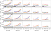 |
Fig. 4. Half-mass radius, R*, 1/2 plotted against M⋆. The rows show variations in the two SN-related parameters ASN1 and ASN2 and the two AGN parameters BHRE and QT. The green lines represent the reference CAMELS simulation. Simulation snapshots at z = 0, z = 0.5, z = 1, z = 1.5, and z = 2 are displayed from left to right. The medians in stellar mass bins are shown. The dark and light grey regions indicate radii smaller than the softening length ϵmin and 2 × ϵmin, respectively. |
Interestingly, for both the correlations the golden mass is absent at z = 2 for any set of parameters, except for extreme values of the AGN-feedback parameters. It first emerges at z ∼ 1 − 1.5 for high values of wind energy and velocity, and only at z = 0 for the lowest values of SN parameters. For extreme values of some AGN feedback parameters it emerges at z ∼ 2, for other at lower redshifts, in some cases it never appears. As an example, it emerges at z = 1.5 − 2 only for the smallest values of BHRE, and only at z = 0 for low values of BHaccr or QT and high values of BHRE. This is suggesting a link to the quenching of galaxies. In all cases where the golden mass is observed, it becomes more consolidated over cosmic time. This emergence is also related to the behavior of the most massive galaxies, which begin to show a positive correlation between DM fraction and mass only between z = 1 and z = 2. Stronger feedback halts star formation, creating galaxies with smaller stellar masses and leading to a higher DM fraction. Star formation quenching and mergers contribute to the increase in size and DM fraction in the most massive galaxies over cosmic time. A more systematic analysis of the size-mass relation as a function of redshift, and the comparison with observations, are beyond the scope of this paper and will be analysed in future papers.
Although we have selected only galaxies with R⋆, 1/2 > ϵmin, some residual resolution effects may still persist above this threshold. To assess their potential impact, in Fig. 4 we highlight sizes below the softening length (excluded from our sample) and those below twice the softening length, across different redshifts. Overall, the vast majority of simulations–across stellar masses and redshifts–would not be affected by resolution limitations. However, exceptions arise in specific cases, such as simulations with very low values of ASN1 or very high values of ASN2 at z ≲ 0.5. Overall, these exceptions may impact the scaling relations at the low-mass end–below the golden mass–but they do not affect our main conclusions.
4.2. Galaxy type dependency
Different types of galaxies are influenced by different processes and span different ranges of masses. Therefore, it is crucial to investigate whether scaling relations differ between these galaxy types. Figure 5 shows the relation between MDM, 1/2/M⋆, 1/2 and M⋆ for PGs and SFGs.
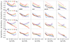 |
Fig. 5. MDM, 1/2/M⋆, 1/2 plotted against M⋆. The rows show variations in the two SN-related parameters ASN1 and ASN2 and the two AGN parameters BRE and QT. The green lines represent the reference CAMELS simulation. Simulation snapshots at z = 0, z = 0.5, z = 1, z = 1.5, and z = 2 are displayed from left to right. The sample is divided in PGs (solid lines) and SFGs (dashed lines). The medians in stellar mass bins are shown. The binning in the two subclasses has been optimized based on the number of points in the bin, and trends based on very few data points have been omitted. |
It is not surprising that the scaling relation for masses larger than the golden mass is predominantly driven by PGs. This is because the number density of star-forming galaxies decreases significantly at ∼ 1010.5−11 M⊙. Additionally, due to our selection criterion of constant sSFR with redshift, the number of PGs at z = 2 is notably low.
For any values of the parameters shown, the variation in central DM fraction with redshift is weaker for SFGs compared to PGs. The stronger variation observed in PGs is favoured by their greater size evolution. Except for the z = 0 snapshot, at fixed stellar mass, the DM fractions of SFGs are generally higher than those of PGs. The impact of SN feedback parameters remains consistent when galaxy types are explicitly considered. The trends observed for the entire sample at high masses apply to PGs, while some differences emerge at low masses and for SFGs.
In SFGs, the decreasing trend with M⋆ of the DM fraction is confirming the results obtained with data both at low- and high-z (Tortora et al. 2019; Sharma et al. 2022). Although the number density of SFGs approaches zero at high masses, a slight change in slope and the emergence of the golden mass is observed for extreme values of some parameters5. Some mild evidence of bending was found in Tortora et al. (2019), using SPARC star-forming galaxies with measured rotation curves (Lelli et al. 2016), tending to exclude simulations with very extreme values of SN- and AGN-feedback parameters. However, the presence of the bend found in observations contrasts with findings in Posti et al. (2019), which, using the sample used in Tortora et al. (2019), reported (relying on global quantities) no bending in the relation between stellar fraction (of star formation efficiency) and stellar mass in the most massive spirals.
To resolve this discrepancy or at least discover the possible cause, it is important to examine the simulations’ predictions for the correlation between the total M⋆/MDM and M⋆, the stellar-to-halo mass relation, obtained including all particles in the subhalos. The results are presented in Fig. 6.
We confirm the maximum in the relation when all galaxies are considered (e.g. Moster et al. 2010), which mirrors the trends observed for central DM fraction as a function of stellar mass (e.g. Fig. 2). The peak of this relation, or the golden mass, increases with higher redshifts. In the highest redshift bin, we observe a flattening at high masses. Models with higher wind energy and velocity tend to have larger central DM fraction, and lower global stellar fractions M⋆/MDM, indicating lower star formation efficiency. Similarly to Fig. 2, varying ASN2 influences the golden mass, whereas varying ASN1 has a smaller effect. Similitude with Fig. 3 can also be made by comparing the trends for AGN-feedback parameters shown in terms of scaling relation normalization and variation in the golden mass value. Limitations due to resolution and simulation volume are investigated in Appendix B, where we also compare with some semi-empirical SHMR from the literature. Except for some shift induced by the smaller resolution of our simulations and the lower number of massive galaxies, the results are quite conform to the original TNG simulations, while some disagreement emerge between both CAMELS and TNG simulations with literature results using halo abundance matching (Moster et al. 2010, 2013; Girelli et al. 2020).
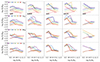 |
Fig. 6. M⋆/MDM plotted against M⋆. The rows show variations in the two SN-related parameters ASN1 and ASN2 and the two AGN parameters BHRE and QT. The green lines represent the reference CAMELS simulation. Simulation snapshots at z = 0, z = 0.5, z = 1, z = 1.5, and z = 2 are displayed from left to right. The sample is divided in PGs (solid lines) and SFGs (dashed lines). Thin lines are used for the median of the full sample. The medians in stellar mass bins are shown. |
For SFGs alone, indications of a golden mass are observed (although very weak), for example in models with high ASN1 and QT values, which contradicts the findings of Posti et al. (2019). The absence of bending in the Posti et al. (2019) results would favour models with a weaker feedback. However, a larger volume would be beneficial to better sample the most massive end of the mass function where LTGs are extremely rare.
An interesting result pertains to the PG population. When considering global quantities, the stellar fraction in our case, no clear bending at the golden mass is observed. In contrast, there are mild indications of a peak at lower masses (∼ 109.5−10 M⊙), which increases for larger (smaller) values of, for example, BHRE (QT). This contrasts with the analysis of the central quantities, where the golden mass clearly emerges for the whole sample and PGs alone, driven by the bending observed in the size-mass relation in both samples (Fig. 5). This may be attributed to the fact that, on global scales, SN and AGN feedback have not yet had sufficient time to take effect.
At low stellar masses (≲ 1010−10.5 M⊙) PGs are characterized by lower halo masses with respect to SFGs of similar stellar masses. Instead, at larger masses halo masses of the two types are quite similar, with many simulations showing some mild indications of larger halo masses in SFGs. Except for the highest-masses in some of our simulations, for the rest we find results opposite to the literature (Rodríguez-Puebla et al. 2015; Correa & Schaye 2020). These results are qualitatively unaffected by a change in the sSFR threshold. We have also explored the impact on the trends of a different classification based on the ratio Vmax/σ, finding that, both cold late-type systems (low Vmax/σ) and hot early-type systems (high Vmax/σ) follow a similar trend with stellar mass, with larger stellar fractions in the former, which looks more consistent with results from Rodríguez-Puebla et al. (2015). In future analyses, we will explore the origin of this result in greater detail.
5. Discussion
The CAMELS simulations are constructed by varying a range of parameters associated with SN and AGN feedback. We have leveraged this flexibility to investigate how these parameters influence the MDM/M⋆–M⋆ scaling relation and the emergence of the golden mass, defined as the stellar mass corresponding to the minimum of this relation, across different redshifts.
Our analysis shows that cosmological parameters do not affect the golden mass. In contrast, several feedback-related parameters–particularly those governing supernova wind velocity and energy, as well as AGN feedback (in particular the fraction of accreted rest mass energy released, the Eddington ratio, and the normalization factor for the AGN energy feedback in the high-accretion state)–play a significant role in shaping this feature. Except in cases where the fraction of accretion rest mass (BHRE) is extremely low, the minimum in the scaling relation persists, allowing the golden mass to be identified up to z ∼ 2. For the remaining parameter variations, the golden mass consistently emerges from z = 1 onwards.
Before proceeding, we caution that beyond z ∼ 1, the limited simulation volume leads to a sharp decline in the number of galaxies with stellar masses above ∼ 1011 M⊙. This scarcity makes the identification of the golden mass increasingly uncertain–and potentially infeasible–at higher redshifts. Addressing this limitation requires simulations with larger volumes. To explore this issue, we derived the corresponding scaling relations using the Illustris TNG100-1 and TNG-300-1 simulations (Nelson et al. 2019b), which contain .approximately 3.4 and 69 times more galaxies than the CAMELS simulations analysed here, in Appendix B. We find that the shape of the scaling relations and the position of the golden mass are broadly consistent between TNG and CAMELS simulations. A similarity between TNG300-1 and CAMELS is expected due to their comparable resolution; however, it is particularly encouraging that the golden mass remains consistent even in the higher-resolution TNG100-1 simulation. The larger volumes of TNG100-1 and TNG300-1, however, enables the golden mass to be probed more robustly at z ≳ 1.
In this section we collect and present the results of the paper using CAMELS simulations in Fig. 7, where our golden mass estimates are compared with results from other simulations and different observational data. We discuss these results in the context of virial shocks, cold gas streams, and feedback from SN and AGN.
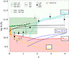 |
Fig. 7. Golden mass determined from the central MDM/M⋆ − M⋆ relation assuming the reference CAMELS simulation (green line) is compared with other results from the literature. A qualitative range for the golden mass values determined from all the CAMELS simulations explored in this paper are shown as dark and light green regions (see text for more details). We also plot the results for the simulations corresponding to the lowest BHRE and highest ASN1 values. Then, we compare with the golden mass estimated from the same correlation for the TNG100-1 (dark green line) and TNG300-1 (dashed dark green line) simulations. From the theoretical point of view, we also show the shock heating stellar mass (Mshock) as a red line and the stream mass (Mstream) as solid cyan line (Dekel & Birnboim 2006), together with its two revised forms (dashed and dotted cyan lines) discussed in Daddi et al. (2022a). These curves for Mshock and Mstream are extracted from Daddi et al. (2022a), where more details can be found. The stream mass determined in Waterval et al. (2025) is also plotted as blue and dark blue lines (see details in the text). We show the typical mass above which SN feedback interrupts its quenching effect, using two conversions from halo to stellar mass (MSN, yellow lines; see text for details). From the observational point of view, we plot the range of golden masses in the local Universe from different observables (Tortora et al. 2010, 2016, 2019). Then, we also plot the stellar mass value of the bending in the SHMR determined from using halo-abundance matching in Moster et al. (2010, black dashed line), Moster et al. (2013, black solid line) and Girelli et al. (2020, grey solid line), and the bending mass in the main sequence of star-forming galaxies (Lee et al. 2015; Delvecchio et al. 2021; Euclid Collaboration: Enia et al. 2025). |
5.1. Different mass scales from simulations and observations
As discussed in Sect. 2, simulations suggest that above a virial mass of Mshock ∼ 1011.7 M⊙, virial shocks heat the CGM, thereby suppressing new star formation. However, at z ≳ 1.5, cold gas streams are expected to continue fueling star formation in halos below a characteristic mass scale, Mstream, which increases with redshift. Consequently, we expect galaxies to be predominantly passive above Mshock at z ≲ 1.5, and above Mstream at higher redshifts. These trends are illustrated in Fig. 7, where halo masses Mshock and Mstream have been converted into stellar masses following Daddi et al. (2022a, Figure 2, left panel). For completeness, we also include the results from Waterval et al. (2025), who use cosmological hydrodynamical simulations from the High-z Evolution of Large and Luminous Objects (HELLO) and the Numerical Investigation of a Hundred Astrophysical Objects (NIHAO) projects. We convert the stream halo mass trend in their Figure 14 into stellar mass, using the SHMR in Girelli et al. (2020, blue) and Moster et al. (2013, darker blue). Interestingly the stream mass in Waterval et al. (2025) is about 1 dex smaller than the Dekel & Birnboim (2006) and Daddi et al. (2022a) relations. In the following we mostly refer to the Dekel & Birnboim (2006) and Daddi et al. (2022a) relations.
By analysing the bending of the SFR–stellar mass relation along the main sequence of star-forming galaxies, Daddi et al. (2022a)–building on measurements from Lee et al. (2015) and Delvecchio et al. (2021)–found that the characteristic bending mass increases with redshift, from ∼ 1010 M⊙ at z ∼ 0.35 to ∼ 1011 M⊙ at z ∼ 2 and beyond (see also Euclid Collaboration: Enia et al. 2025 for consistent results). Their bending mass seems to follow the redshift evolution of Mstream (or its revised versions obtained in Daddi et al. 2022a). Their analysis suggests that the main sequence bending is driven by a decline in cold gas accretion, which limits the fuel available for SF–a scenario consistent with the cold-stream model. Above the Mshock − Mstream mass threshold, the gas supply dwindles, leading to a plateau in the star formation rate rather than an abrupt quenching. Importantly, Daddi et al. (2022a) argue that quenching is governed by additional physical mechanisms beyond the suppression of cold accretion. They also emphasize that the characteristic mass associated with the bending of the main sequence differs from the knee of the stellar mass function, which tends to be higher at z ≲ 1.5.
However, their study does not include a direct measurement of the main sequence bending at z ∼ 0. By extrapolating the observed trends, we may estimate that the bending mass at z ∼ 0 likely falls within the range ∼109.5–1010 M⊙. Interestingly, this scale seems to be different from the typical golden mass values quoted in the literature (see Sect. 2). The bending mass, instead, resembles the first mass scale proposed by Kannappan et al. (2013), who identified a transition mass at z ∼ 0 separating an accretion-dominated regime from a processing-dominated one, where the galaxies start processing the remaining available gas reservoir. These initial considerations prompt us to raise a cautionary note regarding the definition of mass scales, as the transition mass observed in the star-forming main sequence–identified as the “gas-richness threshold” by Kannappan et al. (2013)–may not correspond to the same physical scale as the transition mass investigated in this work, which resembles the “bimodality mass” described in the same study.
In fact, plotting the stellar mass corresponding to the bending of the SHMR results from halo abundance matching (Moster et al. 2010, 2013; Girelli et al. 2020), we see that this mass value aligns better with numerous observational findings in the local Universe, particularly with the range of golden mass values identified through minima in colour gradients (Tortora et al. 2010), as well as through trends in stellar mass of total mass density slopes and DM fractions (Tortora et al. 2016, 2019).
Looking at the evolution with redshift, contrasting results are found. We see a mild evolution in Moster et al. (2010) and Moster et al. (2013), with a flattening at z ≳ 1, A notable discrepancy arises when comparing these values with the shock and stream transition masses Mshock and Mstream. While at z ≲ 1.5 the star formation efficiency peak lies above Mshock, at higher redshifts it falls between Mshock and Mstream–a regime where cold gas flows are still expected to sustain star formation. This contrasts with the consideration that the peak of the star formation efficiency separate mostly passive and star-forming systems. Differently, the more recent results in Girelli et al. (2020), present a stronger evolution with redshift, reaching a value of ∼ 1011 M⊙ at z ∼ 3, and aligning with the Mstream redshift evolution above z ∼ 2. The SHMR for these papers are plotted in Fig. B.1.
In this work, we have provided a new set of predictions for the golden mass, identified as the minimum in the MDM/M⋆–M⋆ scaling relation. Across our suite of simulations, this minimum typically falls within the range ∼1010.3–1011.1 M⊙ at z ≲ 2 (darker green region in Fig. 7, Table 4). We cannot exclude that in a few extreme cases the mass can extend to even higher masses, though these lie in a regime where our simulations become increasingly limited due to low statistics (lighter green region in Fig. 7). At higher redshifts, most simulations do not exhibit a clear minimum in the relation, aside from a few outliers. This absence may reflect the genuine disappearance of the golden mass at early times or may indicate that its detection requires larger-volume simulations capable of massive systems with M⋆ ≳ 1011 M⊙.
In particular, to investigate the impact of the low galaxy statistics at large mass, we compare the trends from the CAMELS reference run with the TNG300-1 and TNG100-1 simulations, obtained with the central MDM/M⋆–M⋆ relation. The SHMRs for these simulations are compared in Fig. B.1. In Fig. 7 we can see that, as expected, the golden mass for CAMELS, TNG100-1 and TNG300-1 are quite the same, confirming the goodness of CAMELS simulations, although the limited volume. Therefore, at z ∼ 0 CAMELS and TNG simulations predict golden mass values that are systematically 0.1–0.2 dex higher than those inferred from observations (Tortora et al. 2010, 2019; Moster et al. 2013), and far more larger than the bending mass in the star formation main sequence. The trends with reshifts look quite similar to halo abundance matching results in Girelli et al. (2020). Also using the higher volume and resolution of TNG100-1 and the much more larger volume of TNG300-1, at z ≳ 1.5 − 2 no golden mass is found, and therefore it is natural to expect the same in simulations with similar or weaker SN and AGN feedback. No conclusion can be drawn for extreme strong feedback models.
Thanks to their larger volumes, the golden mass can be traced in TNG300-1 and TNG100-1 up to z ∼ 1.5, compared to the more limited range of z ∼ 0.5 − 1 accessible with the reference CAMELS simulation. These findings suggest that future studies would benefit from running CAMELS simulations in larger volumes, which would enable more robust tracking of redshift evolution and better characterization of the impact of varying SN and AGN feedback parameters.
The range of the golden mass in CAMELS and TNG simulations however seems to be within the region above Mshock − Mstream, where the availability of cold gas is limited.
5.2. Feedback, shocks and streams: Competing or alternative processes
We need to determine whether these results imply that our simulations are consistent with the shock-stream scenario, and whether virial shocks and cold streams are the fundamental drivers behind the emergence of the golden mass in the scaling relation or if these processes are acting in a complementary way. Furthermore, discrepancies might arise from the use of different mass definitions across studies.
We have shown and discussed that SN and AGN feedback parameters have a significant impact on the emergence of the golden mass. In particular, when the strength of SN and AGN feedback is reduced, the minimum in the scaling relations–even at z ∼ 0–tends to disappear. While we do not have access to simulations in which these feedback mechanisms are completely turned off, the trends observed in our results strongly suggest that such a scenario would likely prevent the formation of a well-defined golden mass. This reasoning is performed at z ≲ 0.5, where limitations due to the simulated volume are not affecting our inferences. However, these considerations seem to also hold at larger redshifts up to z ∼ 1.5 − 2, considering the higher volume and resolution of the original TNG simulations. We can extrapolate these results to hypothetical TNG simulations with weaker feedback models at z ≳ 1.5 − 2. This indicates that, on their own, shock and stream processes alone may not be sufficient to produce the minima seen in our scaling relations–at least within the CAMELS framework using the Illustris TNG subgrid model.
Further analysis is needed to disentangle the roles of these two feedback processes. At low stellar masses, SN feedback is known to be the dominant mechanism regulating star formation (Nelson et al. 2019a; Weinberger et al. 2018). Theoretical considerations (e.g. Dekel & Silk 1986) provide an estimate for the upper halo mass where SN feedback remains effective, MSN = MSN, 0(1 + z)−3/2. Assuming MSN,0 = 1011.7 M⊙, after converting this halo mass to a stellar mass, following Daddi et al. (2022a), we find a corresponding value of ∼ 1010.2 M⊙ at z = 0, which decreases rapidly with redshift to ∼ 109.5 M⊙ at z ∼ 2 (shown as solid yellow line in Fig. 7). A slightly different trend is found if the Moster et al. (2013) SHMR is used to convert from halo to stellar mass (dashed yellow line). However, this trend disagrees with our findings, since in Fig. 2, we also see that modifying SN feedback parameters can influence the scaling relation across a broad mass range, up to M⋆ ∼ 1011.5 M⊙. While the effect of wind velocity appears to diminish in massive galaxies at high redshift, wind energy continues to have a strong impact on galaxies at all masses and redshifts. This mass scale is much more larger than the MSN mass estimated by the above-mentioned theoretical calculations.
AGN feedback, in contrast, becomes increasingly dominant at higher stellar masses. It not only expels gas from central regions but also heats it significantly, driving powerful outflows, as shown in TNG simulations (Nelson et al. 2019a; Weinberger et al. 2018; Terrazas et al. 2020; Zinger et al. 2020). Our parameter studies confirm that the influence of AGN feedback grows with mass, becoming particularly relevant at M⋆ ≳ 1010 M⊙ in most of the models examined.
Finally, it is important to know whether we can constrain the strength of feedback processes. At this stage, we cannot fully adopt the methodology used in the previous CASCO papers, as we do not yet have the large ensemble of CAMELS simulations in which cosmological and astrophysical parameters are finely, uniformly and randomly sampled. Instead, we are limited to the 1P simulations, where only one parameter is varied at a time. We defer a more robust statistical analysis to a future study, once the full set of simulations becomes available. Nonetheless, we can offer some qualitative constraints by comparing the golden mass derived from the 1P simulations with observational benchmarks. Currently, central DM-to-stellar mass relations are primarily available at z ∼ 0, while at higher redshifts the limited mass range probed by observations makes it difficult to constrain the bending mass systematically. For this reason, we focus on the local Universe, comparing our results to the typical golden mass inferred from local central DM-to-stellar mass relations and other datasets (represented by the thick orange vertical line in Fig. 7).
A comparison with the higher-resolution reference TNG100-1 simulation shows that resolution has only a mild effect on the inferred golden mass in CAMELS, which allows us to neglect this source of systematics, which seems to have a larger effect on the normalization of the SHMR at fixed stellar mass, as seen in Fig. B.1. To match the observed golden mass values at z ∼ 0 or approach them, one would need to strengthen the effects of SN or AGN feedbacks. This could be achieved, for instance, by maximizing one of the SN feedback parameters (ASN1 or ASN2), reducing the value of the BH radiative efficiency BHRE to its lowest simulated level, or increasing the quasar threshold QT. The results for the highest ASN1 and lowest BHRE simulation are also shown for comparison in Fig. 7.
5.3. A unified scenario
Although both simulations and data require further refinement, the results summarized in Fig. 7 allow us to draw several overarching conclusions. The golden mass derived from the reference CAMELS simulation, along with results from TNG100-1, TNG300-1, and the recent halo abundance matching analysis by Girelli et al. (2020), are broadly consistent up to z ∼ 1.5. Above this redshift, also the TNG simulations no longer show a bending in the SHMR, whereas the golden mass from Girelli et al. (2020) continues to increase with redshift, eventually overlapping with the Mstream threshold beyond z ∼ 2.
At these high redshifts, the bending mass in the star-forming main sequence also aligns with Mstream, indicating that the maximum of star formation efficiency, the main sequence bending mass, and the cold-streaming threshold all converge onto the same physical mass scale. Conversely, below z ∼ 2, various simulations and observations–including those examining the SHMR (e.g. Girelli et al. 2020), the minimum in the DM fraction–stellar mass correlation in CAMELS and TNG, and different observations of local galaxies (e.g. Tortora et al. 2019)–point to a characteristic mass scale, which we refer to as the golden mass, in the range log M⋆/M⊙ ∼ 10.2–10.6.
However, the bending mass of the main sequence at low redshift decreases more steeply, reaching values of log M⋆/M⊙ ∼ 9.5–10, consistent with the gas-richness threshold identified by Kannappan et al. (2013).
In summary, above z ∼ 2, a single characteristic mass scale appears to mark the shutdown of gas accretion, leading to quenching, morphological transformation, and the emergence of red, spheroid-dominated galaxies. Below this redshift, instead, two mass scales are emerging, one tied to the gas availability, the “gas-richness” threshold, and the second to star formation quenching, i.e. the bimodality or golden mass.
6. Conclusions
In this paper we investigated the emergence of what is known as the golden mass, by studying the scaling relation between MDM, 1/2/M⋆, 1/2, the ratio of total-to-stellar mass within the half-mass radius (equivalent to a DM fraction), and stellar mass. We utilized a new suite of CAMELS simulations that enhanced previous simulations by increasing the volume to (50 h−1 Mpc)3, thus allowing for a more detailed examination of the most massive end of the galaxy mass function (Villaescusa-Navarro et al. 2021, 2023; Ni et al. 2023). These simulations enabled us to analyse the impact of various astrophysical and cosmological parameters, including SN and AGN feedback strengths as well as Ωm and σ8, across different redshifts. However, we note that larger volume simulations would be beneficial in order to determine whether a golden mass appears at masses greater than 1011 M⊙ at large redshifts.
For most astrophysical and cosmological parameter values across various redshifts, the MDM, 1/2/M⋆, 1/2–M⋆ relation follows a U-shaped curve, indicating the presence of a golden mass at the minimum of the curve (Tortora et al. 2019). However, at high redshifts, such as z = 2, this ratio decreases with stellar mass, and no golden mass is observed.
Cosmological parameters primarily influence the normalization of this scaling relation, but do not affect the emergence of the golden mass. The U-shaped trend becomes more pronounced with higher values of supernova feedback energy (ASN1) and wind velocity (ASN2); the latter has a stronger impact on the golden mass value. Our findings confirm that while the normalization factors for AGN energy and event frequency (AAGN1 and AAGN2) have only minor or negligible effects on the scaling relations, other AGN feedback-related parameters implemented in the CAMELS simulations play a more significant role. Specifically, larger values of the normalization factor for the Bondi rate for the accretion onto BHs (BH accretion rate BHaccr), the normalization factor for the limiting Eddington rate for the accretion onto BHs (Eddington factor BHEdd), the Eddington ratio that serves as the threshold between the low-accretion and high-accretion states of AGN feedback (quasar threshold QT), and the power-law index of the scaling of the low- to high-accretion state threshold with BH mass (quasar threshold power QTP) increase DM fractions at high masses and induce a bend in the scaling relation, while factors such as the normalization factor for the energy in AGN feedback, per unit accretion rate, in the high-accretion state (BH feedback factor BHFF) and the fraction of the accretion rest mass that is released in the accretion process (BH radiative efficiency BHRE) work in the opposite direction.
In summary, the fraction of the accretion rest mass that is released in the accretion process is the parameter that has the most impact on the golden mass value, followed by the normalization factor for the energy in AGN feedback, the threshold between the low-accretion and high-accretion states of AGN feedback, and SN wind velocity. The rest of the parameters induce milder trends or no trends.
In PGs, the U-shaped curve is clearly visible in the MDM, 1/2/M⋆, 1/2–M⋆ relation, while SFGs display a monotonically decreasing trend with stellar mass across all redshifts, with only mild indications of a turnover at very low redshifts. These results align with observational findings (Tortora et al. 2016, 2019). In SFGs, DM fractions decrease over cosmic time, while PGs show a significant increase, particularly in the most massive systems where size evolution contributes to the rise in central DM fractions (e.g. Tortora et al. 2014, 2018). Models with stronger SN and AGN feedback demonstrate faster evolution in both size and DM fractions.
Regarding global quantities, SFGs dominate the scaling relation below the golden mass and exhibit only marginal bending, which becomes more pronounced with stronger wind energy. PGs dominate at higher masses, but do not show a sharp peak at the golden mass. Instead, they exhibit a mild peak around 109.5−10 M⊙ (changing to larger values for extreme values of some AGN feedback parameters) and a decreasing trend at higher masses, a pattern that warrants further observational testing. While there are some hints of bending in the central and global properties of SFGs, larger-volume simulations are needed to explore the massive end of the mass function and to further investigate the star formation efficiency in the most massive spiral galaxies (Posti et al. 2019; Tortora et al. 2019).
We have finally discussed our results in a broader context, comparing them with mass variations predicted in the shock-stream scenario, together with literature results from the stellar-to-halo mass relation and the main sequence of star-forming galaxies. Our results point to the predominant role of SN and AGN feedback in leading the scaling relations, with SN feedback impacting also the most massive galaxies. From the comparison with the literature, however, some possible discrepancies emerge on the association of the bending mass of the main sequence and the minima of our scaling relations, which are possibly two distinct mass scales (as also Daddi et al. 2022a was reporting). We believe that the bending mass in the main sequence is equivalent to the gas-richness mass mentioned in Kannappan et al. (2013), separating accretion-dominated from processing-dominated galaxies, while the minima in our scaling relations are more connected to morphological differences and a quenching of star formation rather than on the availability of gas. We speculate that above z ∼ 2, all these characteristic mass scales converge, likely coinciding with the cold-streaming threshold mass (Mstream). Below this redshift, however, two distinct mass scales emerge: the gas-richness threshold at ∼109.5 − 10 M⊙, and the bimodality or golden mass at ∼1010.2 − 10.6 M⊙.
In future papers, following the procedure in Papers I and II, we will constrain these new simulations with this extended list of simulation parameters with observations (star-forming galaxies: Tortora et al. 2019; passive galaxies: Tortora et al. 2012; Zhu et al. 2023), weighting the role of SN and AGN feedback. Among the new data available, the Euclid mission’s > 100 000 strong lenses (Euclid Collaboration: Mellier et al. 2025; Acevedo Barroso et al. 2025; Euclid Collaboration: Walmsley et al. 2025), combined with weak lensing signals from stacked lenses and spectroscopic follow-ups (e.g. Collett et al. 2023), will provide precise data on central DM and total virial mass across a broad mass range and up to z = 2, allowing physical processes to be constrained, and in particular providing AGN feedback (e.g. Mukherjee et al. 2021), which is one of the most dominant phenomena in very massive galaxies. Moreover, discovering several systems with spiral galaxies as lenses will also help address questions about the star formation efficiency of the most massive spiral galaxies across cosmic time, constraining the golden mass as a function of time and galaxy type.
We limit the analysis to a Chabrier (2003) IMF, deferring the investigation of the IMF’s impact on stellar mass and DM fraction to a future paper (see more on the IMF in Tortora et al. 2009, 2013).
In physical units, the softening length takes the following values: 2.0, 1.3, 0.978, 0.806, and 0.666 kpc at redshifts z = 0, 0.5, 1.0, 1.5, and 2, respectively.
In our previous papers we adopted a different nomenclature–referring to early-type and late-type galaxies instead of passive and star-forming–even though the same selection criterion was applied. This choice was motivated by the direct comparison with observational data, which were classified primarily based on morphology rather than star formation activity.
Using Mtot, 1/2/M⋆, 1/2 instead of MDM, 1/2/M⋆, 1/2 increases the golden mass by less than 0.05–0.1 dex without affecting our conclusions.
In some panels, the same binning used across simulations obscures the detection of this bending.
Acknowledgments
We thank the referee for their insightful comments, which have significantly enhanced the clarity and quality of our manuscript. C. T. thanks Carlo Cannarozzo for the useful discussions during IAU Symposium #396. C.T. and V.B. acknowledge the INAF grant 2022 LEMON.
References
- Acevedo Barroso, J. A., O’Riordan, C. M., Clément, B., et al. 2025, A&A, 697, A14 [Google Scholar]
- Aquino-Ortíz, E., Valenzuela, O., Sánchez, S. F., et al. 2018, MNRAS, 479, 2133 [Google Scholar]
- Aung, H., Mandelker, N., Dekel, A., et al. 2024, MNRAS, 532, 2965 [NASA ADS] [CrossRef] [Google Scholar]
- Behroozi, P. S., Wechsler, R. H., & Conroy, C. 2013, ApJ, 762, L31 [NASA ADS] [CrossRef] [Google Scholar]
- Behroozi, P., Wechsler, R. H., Hearin, A. P., & Conroy, C. 2019, MNRAS, 488, 3143 [NASA ADS] [CrossRef] [Google Scholar]
- Benson, A. J., Cole, S., Frenk, C. S., Baugh, C. M., & Lacey, C. G. 2000, MNRAS, 311, 793 [NASA ADS] [CrossRef] [Google Scholar]
- Bisigello, L., Kuchner, U., Conselice, C. J., et al. 2020, MNRAS, 494, 2337 [NASA ADS] [CrossRef] [Google Scholar]
- Bower, R. G., Schaye, J., Frenk, C. S., et al. 2017, MNRAS, 465, 32 [NASA ADS] [CrossRef] [Google Scholar]
- Busillo, V., Tortora, C., Napolitano, N. R., et al. 2023, MNRAS, 525, 6191 [NASA ADS] [CrossRef] [Google Scholar]
- Busillo, V., Tortora, C., Covone, G., et al. 2025, A&A, 693, A112 [NASA ADS] [CrossRef] [EDP Sciences] [Google Scholar]
- Capaccioli, M., Caon, N., & D’Onofrio, M. 1992, MNRAS, 259, 323 [NASA ADS] [CrossRef] [Google Scholar]
- Cappellari, M., McDermid, R. M., Alatalo, K., et al. 2013, MNRAS, 432, 1862 [NASA ADS] [CrossRef] [Google Scholar]
- Chabrier, G. 2003, PASP, 115, 763 [Google Scholar]
- Chawak, C., Villaescusa-Navarro, F., Echeverri Rojas, N., et al. 2023, arXiv e-prints [arXiv:2309.12048] [Google Scholar]
- Collett, T. E., Sonnenfeld, A., Frohmaier, C., et al. 2023, The Messenger, 190, 49 [Google Scholar]
- Conroy, C., & Wechsler, R. H. 2009, ApJ, 696, 620 [NASA ADS] [CrossRef] [Google Scholar]
- Correa, C. A., & Schaye, J. 2020, MNRAS, 499, 3578 [Google Scholar]
- Courteau, S., Cappellari, M., de Jong, R. S., et al. 2014, Rev. Mod. Phys., 86, 47 [Google Scholar]
- Daddi, E., Delvecchio, I., Dimauro, P., et al. 2022a, A&A, 661, L7 [NASA ADS] [CrossRef] [EDP Sciences] [Google Scholar]
- Daddi, E., Rich, R. M., Valentino, F., et al. 2022b, ApJ, 926, L21 [NASA ADS] [CrossRef] [Google Scholar]
- de Jong, R. 2011, The Messenger, 145, 14 [NASA ADS] [Google Scholar]
- Dekel, A., & Birnboim, Y. 2006, MNRAS, 368, 2 [NASA ADS] [CrossRef] [Google Scholar]
- Dekel, A., & Silk, J. 1986, ApJ, 303, 39 [Google Scholar]
- Dekel, A., Lapiner, S., & Dubois, Y. 2019, arXiv e-prints [arXiv:1904.08431] [Google Scholar]
- Delvecchio, I., Daddi, E., Sargent, M. T., et al. 2021, A&A, 647, A123 [NASA ADS] [CrossRef] [EDP Sciences] [Google Scholar]
- Donnari, M., Pillepich, A., Nelson, D., et al. 2019, MNRAS, 485, 4817 [Google Scholar]
- D’Onofrio, M., Marziani, P., & Chiosi, C. 2021, Front. Astron. Space Sci., 8, 157 [Google Scholar]
- Dubois, Y., Volonteri, M., Silk, J., et al. 2015, MNRAS, 452, 1502 [Google Scholar]
- Dutton, A. A., Conroy, C., van den Bosch, F. C., Prada, F., & More, S. 2010, MNRAS, 407, 2 [Google Scholar]
- Euclid Collaboration (Enia, A., et al.) 2025, A&A, in press http://doi.org/10.1051/0004-6361/202554576 [Google Scholar]
- Euclid Collaboration (Mellier, Y., et al.) 2025, A&A, 697, A1 [Google Scholar]
- Euclid Collaboration (Walmsley, M., et al.) 2025, A&A, submitted, [arXiv:2503.15324] [Google Scholar]
- Ginolfi, M., Hunt, L. K., Tortora, C., Schneider, R., & Cresci, G. 2020, A&A, 638, A4 [NASA ADS] [CrossRef] [EDP Sciences] [Google Scholar]
- Girelli, G., Pozzetti, L., Bolzonella, M., et al. 2020, A&A, 634, A135 [NASA ADS] [CrossRef] [EDP Sciences] [Google Scholar]
- Habouzit, M., Genel, S., Somerville, R. S., et al. 2019, MNRAS, 484, 4413 [CrossRef] [Google Scholar]
- Hahn, C., Starkenburg, T. K., Choi, E., et al. 2019, ApJ, 872, 160 [NASA ADS] [CrossRef] [Google Scholar]
- Hunt, L. K., Tortora, C., Ginolfi, M., & Schneider, R. 2020, A&A, 643, A180 [NASA ADS] [CrossRef] [EDP Sciences] [Google Scholar]
- Hyde, J. B., & Bernardi, M. 2009, MNRAS, 394, 1978 [NASA ADS] [CrossRef] [Google Scholar]
- Iovino, A., Mercurio, A., Gallazzi, A. R., et al. 2023a, The Messenger, 190, 22 [NASA ADS] [Google Scholar]
- Iovino, A., Poggianti, B. M., Mercurio, A., et al. 2023b, A&A, 672, A87 [NASA ADS] [CrossRef] [EDP Sciences] [Google Scholar]
- Kannappan, S. J., Stark, D. V., Eckert, K. D., et al. 2013, ApJ, 777, 42 [Google Scholar]
- Kereš, D., Katz, N., Weinberg, D. H., & Davé, R. 2005, MNRAS, 363, 2 [Google Scholar]
- Kormendy, J., Fisher, D. B., Cornell, M. E., & Bender, R. 2009, ApJS, 182, 216 [Google Scholar]
- Kuntschner, H., Emsellem, E., Bacon, R., et al. 2010, MNRAS, 408, 97 [Google Scholar]
- Lee, N., Sanders, D. B., Casey, C. M., et al. 2015, ApJ, 801, 80 [Google Scholar]
- Lelli, F., McGaugh, S. S., & Schombert, J. M. 2016, AJ, 152, 157 [Google Scholar]
- Lovell, M. R., Pillepich, A., Genel, S., et al. 2018, MNRAS, 481, 1950 [Google Scholar]
- Marinoni, C., & Hudson, M. J. 2002, ApJ, 569, 101 [NASA ADS] [CrossRef] [Google Scholar]
- More, S., van den Bosch, F. C., Cacciato, M., et al. 2011, MNRAS, 410, 210 [Google Scholar]
- Moster, B. P., Somerville, R. S., Maulbetsch, C., et al. 2010, ApJ, 710, 903 [Google Scholar]
- Moster, B. P., Naab, T., & White, S. D. M. 2013, MNRAS, 428, 3121 [Google Scholar]
- Mukherjee, S., Koopmans, L. V. E., Metcalf, R. B., et al. 2018, MNRAS, 479, 4108 [NASA ADS] [CrossRef] [Google Scholar]
- Mukherjee, S., Koopmans, L. V. E., Metcalf, R. B., et al. 2021, MNRAS, 504, 3455 [NASA ADS] [CrossRef] [Google Scholar]
- Mukherjee, S., Koopmans, L. V. E., Tortora, C., et al. 2022, MNRAS, 509, 1245 [Google Scholar]
- Napolitano, N. R., Capaccioli, M., Romanowsky, A. J., et al. 2005, MNRAS, 357, 691 [Google Scholar]
- Napolitano, N. R., Romanowsky, A. J., & Tortora, C. 2010, MNRAS, 405, 2351 [NASA ADS] [Google Scholar]
- Nedkova, K. V., Häußler, B., Marchesini, D., et al. 2021, MNRAS, 506, 928 [NASA ADS] [CrossRef] [Google Scholar]
- Nelson, D., Pillepich, A., Springel, V., et al. 2019a, MNRAS, 490, 3234 [Google Scholar]
- Nelson, D., Springel, V., Pillepich, A., et al. 2019b, Comput. Astrophys. Cosmol., 6, 2 [Google Scholar]
- Ni, Y., Genel, S., Anglés-Alcázar, D., et al. 2023, ApJ, 959, 136 [NASA ADS] [CrossRef] [Google Scholar]
- Pillepich, A., Springel, V., Nelson, D., et al. 2018, MNRAS, 473, 4077 [Google Scholar]
- Popesso, P., Concas, A., Cresci, G., et al. 2023, MNRAS, 519, 1526 [Google Scholar]
- Posti, L., Fraternali, F., & Marasco, A. 2019, A&A, 626, A56 [NASA ADS] [CrossRef] [EDP Sciences] [Google Scholar]
- Rodríguez-Puebla, A., Avila-Reese, V., Yang, X., et al. 2015, ApJ, 799, 130 [Google Scholar]
- Roy, N., Napolitano, N. R., La Barbera, F., et al. 2018, MNRAS, 480, 1057 [Google Scholar]
- Sharma, G., Salucci, P., & van de Ven, G. 2022, A&A, 659, A40 [NASA ADS] [CrossRef] [EDP Sciences] [Google Scholar]
- Shen, S., Mo, H. J., White, S. D. M., et al. 2003, MNRAS, 343, 978 [NASA ADS] [CrossRef] [Google Scholar]
- Speagle, J. S., Steinhardt, C. L., Capak, P. L., & Silverman, J. D. 2014, ApJS, 214, 15 [Google Scholar]
- Spolaor, M., Kobayashi, C., Forbes, D. A., Couch, W. J., & Hau, G. K. T. 2010, MNRAS, 408, 272 [Google Scholar]
- Stephenson, J., Rodríguez-Puebla, A., Faber, S. M., et al. 2024, MNRAS, 532, 4217 [Google Scholar]
- Stern, J., Fielding, D., Faucher-Giguère, C.-A., & Quataert, E. 2020, MNRAS, 492, 6042 [Google Scholar]
- Terrazas, B. A., Bell, E. F., Pillepich, A., et al. 2020, MNRAS, 493, 1888 [Google Scholar]
- Toloba, E., Boselli, A., Cenarro, A. J., et al. 2011, A&A, 526, A114 [NASA ADS] [CrossRef] [EDP Sciences] [Google Scholar]
- Tortora, C., Napolitano, N. R., Romanowsky, A. J., Capaccioli, M., & Covone, G. 2009, MNRAS, 396, 1132 [NASA ADS] [CrossRef] [Google Scholar]
- Tortora, C., Napolitano, N. R., Cardone, V. F., et al. 2010, MNRAS, 407, 144 [Google Scholar]
- Tortora, C., Napolitano, N. R., Romanowsky, A. J., et al. 2011, MNRAS, 418, 1557 [Google Scholar]
- Tortora, C., La Barbera, F., Napolitano, N. R., de Carvalho, R. R., & Romanowsky, A. J. 2012, MNRAS, 425, 577 [NASA ADS] [CrossRef] [Google Scholar]
- Tortora, C., Romanowsky, A. J., & Napolitano, N. R. 2013, ApJ, 765, 8 [NASA ADS] [CrossRef] [Google Scholar]
- Tortora, C., Napolitano, N. R., Saglia, R. P., et al. 2014, MNRAS, 445, 162 [NASA ADS] [CrossRef] [Google Scholar]
- Tortora, C., La Barbera, F., & Napolitano, N. R. 2016, MNRAS, 455, 308 [Google Scholar]
- Tortora, C., Napolitano, N. R., Roy, N., et al. 2018, MNRAS, 473, 969 [NASA ADS] [CrossRef] [Google Scholar]
- Tortora, C., Posti, L., Koopmans, L. V. E., & Napolitano, N. R. 2019, MNRAS, 489, 5483 [Google Scholar]
- Tully, R. B., & Verheijen, M. A. W. 1997, ApJ, 484, 145 [NASA ADS] [CrossRef] [Google Scholar]
- van den Bosch, F. C., Yang, X., Mo, H. J., et al. 2007, MNRAS, 376, 841 [Google Scholar]
- Villaescusa-Navarro, F., Anglés-Alcázar, D., Genel, S., et al. 2021, ApJ, 915, 71 [NASA ADS] [CrossRef] [Google Scholar]
- Villaescusa-Navarro, F., Genel, S., Anglés-Alcázar, D., et al. 2023, ApJS, 265, 54 [NASA ADS] [CrossRef] [Google Scholar]
- Waterval, S., Cannarozzo, C., & Macciò, A. V. 2025, MNRAS, 537, 2726 [Google Scholar]
- Weinberger, R., Springel, V., Pakmor, R., et al. 2018, MNRAS, 479, 4056 [Google Scholar]
- Whitaker, K. E., Franx, M., Leja, J., et al. 2014, ApJ, 795, 104 [NASA ADS] [CrossRef] [Google Scholar]
- Widrow, L. M., Elahi, P. J., Thacker, R. J., Richardson, M., & Scannapieco, E. 2009, MNRAS, 397, 1275 [Google Scholar]
- Wojtak, R., & Mamon, G. A. 2013, MNRAS, 428, 2407 [Google Scholar]
- Wolf, J., Martinez, G. D., Bullock, J. S., et al. 2010, MNRAS, 406, 1220 [NASA ADS] [Google Scholar]
- Zhu, K., Lu, S., Cappellari, M., et al. 2023, MNRAS, 522, 6326 [NASA ADS] [CrossRef] [Google Scholar]
- Zinger, E., Pillepich, A., Nelson, D., et al. 2020, MNRAS, 499, 768 [CrossRef] [Google Scholar]
Appendix A: Star-forming main sequence compared with the literature
In this paper we distinguished SFGs from PGs adopting a threshold of log(sSFR/yr−1) = − 10.5. However, measuring the SFR is also essential to study one of the most widely explored scaling relations in galaxy evolution: the star-forming main sequence (Speagle et al. 2014; Whitaker et al. 2014; Lee et al. 2015; Ginolfi et al. 2020; Delvecchio et al. 2021; Daddi et al. 2022a; Popesso et al. 2023).
In Fig. A.1, we show the star-forming main sequence for CAMELS galaxies. Differently from the rest of the paper, here we adopt a more conservative threshold of log(sSFR/yr−1) = − 12 to select SFGs. This choice reflects the fact that the main sequence in TNG simulations shows curvature depending on the specific sSFR cut adopted (e.g. Donnari et al. 2019). Nonetheless, applying the same selection used in this section to the other main scaling relations in the paper does not affect our main conclusions.
We find that the energy injected by SN winds (ASN1) has a smaller impact on the normalization of the main sequence compared to wind velocity (ASN2). At fixed stellar mass, higher wind velocities result in lower SFRs. Moreover, using the same sSFR threshold as in the rest of the paper tends to wash out the bending of the main sequence.
Due to the limited volume of our CAMELS boxes, we cannot probe the high-mass end where the bending becomes more prominent. To mitigate this, we compare our results with the larger-volume TNG100-1 and TNG300-1 simulations, which cover volumes 3.4 and 69 times larger, respectively, than the volume used in our CAMELS simulations. TNG100-1 offers higher mass and higher spatial resolution, while TNG300-1 has a resolution comparable to CAMELS. The CAMELS reference simulation is in excellent agreement with these runs at intermediate masses. At higher masses, some discrepancies emerge, likely driven by low number statistics. We also include in the z = 0, z = 1, and z = 2 panels the best-fit relations from Donnari et al. (2019), derived for galaxies in the stellar mass range log M⋆/M⊙ ∈ (9.0–10.5) in TNG300-1. Despite minor differences in the selection criteria, our trends in TNG300-1 match theirs very well.
Finally, we compare our results with empirical fits from Lee et al. (2015) and Delvecchio et al. (2021). These confirm that both the slope and the redshift evolution of the simulated main sequence are broadly consistent with observations. However, the TNG simulations systematically underpredict the SFR of real galaxies by about 0.5 dex. Interestingly, we find that adopting very low values of ASN2 (e.g. ∼0.5) can help reduce this discrepancy. Our results follow the findings in Donnari et al. (2019). For a detailed analysis of the main sequence and the quenched fraction in TNG simulations, we refer the reader to that paper (see also Hahn et al. 2019).
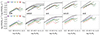 |
Fig. A.1. Star-forming main sequence in the CAMELS simulations as a function of ASN1 (top panels) and ASN2 (bottom panels). To illustrate the redshift evolution, we present simulation snapshots at z = 0, z = 0.5, z = 1, z = 1.5, and z = 2, displayed from left to right. In each panel, we show the median SFR in stellar mass bins. We compare the CAMELS results with those from the larger-volume TNG100-1 (solid dark green) and TNG300-1 (dashed dark green) simulations (Nelson et al. 2019b). The thin dashed blue line represents the best-fit to the main sequence in the stellar mass range log(M⋆/M⊙) = 9–10.5, as derived in Donnari et al. (2019) using TNG300-1. We also include observational results from Delvecchio et al. (2021, solid black line) and Lee et al. (2015, dashed black line) in contiguous redshift bins (extracted from Table 1 in Daddi et al. 2022a). |
Appendix B: The stellar-to-halo-mass relation compared with the literature
The SHMR is one of the most extensively studied scaling relations in the literature. Results for CAMELS simulations, dividing galaxies in PGs and SFGs, are shown in Fig. 6. It is however important to compare our results with existing findings.
As a first step, in Fig. B.1 we compare our results with those obtained using a CAMELS simulation volume of (25 h−1 Mpc)3. This comparison shows that the SHMR remains largely unchanged; however, the smaller volume contains fewer galaxies, which affects the relation, especially at the high-mass end.
We also compared our results with those from the TNG100-1 and TNG300-1 simulations. At fixed stellar mass, TNG100-1 predicts higher halo masses (by ∼0.2–0.3 dex), whereas the SHMR from TNG300-1 more closely matches that from CAMELS. The benefits of the larger simulation volumes in TNG100-1 and TNG300-1 are evident, highlighting a clear path forwards for accurately mapping this and other scaling relations, particularly at the high-mass end.
Finally, we compared our results with semi-empirical models based on halo abundance matching. We invert Equation 2 in Moster et al. (2010) to obtain the correlation between halo and stellar mass, and use best-fitted parameters in Table 7 of Moster et al. (2010), Table 1 of Moster et al. (2013) and Table 3 of Girelli et al. (2020) and the respective functional forms for the evolving parameters with redshifts. The models of Moster et al. (2010) and Moster et al. (2013) predict stronger evolution at z < 0.5 than seen in both CAMELS and TNG, especially at stellar masses ≲ 1010.5 M⊙. At z ∼ 0, Moster et al. (2013) resembles TNG100-1, while at higher redshift they align more closely with CAMELS. Moster et al. (2010) is in better agreement with TNG300-1 and CAMELS. In contrast, the results from Girelli et al. (2020) closely follow TNG100-1 across all redshifts up to ≲ 1010.5 M⊙. Notably, all abundance matching models exhibit a steep decline at the high-mass end, a trend not seen in the TNG and CAMELS simulations, which instead show a more gradual decrease beyond ∼ 1010.5 M⊙.
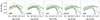 |
Fig. B.1. SHMR of the reference CAMELS simulation with a volume of (50 h−1 Mpc)3 showing the medians in stellar bins (solid green line) and the 16th–84th percentile range (shaded green region). To examine the evolution across redshift, simulation snapshots at z = 0, z = 0.5, z = 1, z = 1.5, and z = 2 are displayed from left to right. It is compared with the same simulation run in a smaller volume of (25 h−1 Mpc)3 (Villaescusa-Navarro et al. 2021, dotted green). We also show results from the TNG100-1 (dark green) and TNG300-1 (dark dashed green) simulations (Nelson et al. 2019b). For both CAMELS and TNG simulations, we plot the medians of the sample distribution divided in stellar mass bins. For comparison with semi-empirical models, we include abundance matching results from Moster et al. (2010, dashed black), Moster et al. (2013, solid black), and Girelli et al. (2020, Table 3, solid grey). |
All Tables
Free parameters of CAMELS simulations used in this paper (for more details, see Ni et al. 2023).
All Figures
|
Fig. 1. MDM, 1/2/M⋆, 1/2 plotted against M⋆ for the CAMELS simulations. Each row shows variations in the cosmological parameters Ωm and σ8. The green lines represent the reference CAMELS simulation. To examine the evolution across redshift, simulation snapshots at z = 0, z = 0.5, z = 1, z = 1.5, and z = 2 are displayed from left to right. The medians in stellar mass bins are shown. For the reference simulation the 16-84th percentile range is also shown as a shaded green region. |
| In the text | |
|
Fig. 2. MDM, 1/2/M⋆, 1/2 plotted against M⋆ for the CAMELS simulations. Each row shows variations in the SN-related parameters ASN1 and ASN2. The green lines represent the reference CAMELS simulation. To examine the evolution across redshift, simulation snapshots at z = 0, z = 0.5, z = 1, z = 1.5, and z = 2 are displayed from left to right. The medians in stellar mass bins are shown. |
| In the text | |
|
Fig. 3. MDM, 1/2/M⋆, 1/2 plotted against M⋆. Each row shows variations in the AGN-related simulation parameters: AAGN1, AAGN2, BHaccr, BHEdd, BHFF, BHRE, QT, and QTP from top to bottom. The green lines represent the reference CAMELS simulation. To examine the evolution across redshift, simulation snapshots at z = 0, z = 0.5, z = 1, z = 1.5, and z = 2 are displayed from left to right. The medians in stellar mass bins are shown. |
| In the text | |
|
Fig. 4. Half-mass radius, R*, 1/2 plotted against M⋆. The rows show variations in the two SN-related parameters ASN1 and ASN2 and the two AGN parameters BHRE and QT. The green lines represent the reference CAMELS simulation. Simulation snapshots at z = 0, z = 0.5, z = 1, z = 1.5, and z = 2 are displayed from left to right. The medians in stellar mass bins are shown. The dark and light grey regions indicate radii smaller than the softening length ϵmin and 2 × ϵmin, respectively. |
| In the text | |
|
Fig. 5. MDM, 1/2/M⋆, 1/2 plotted against M⋆. The rows show variations in the two SN-related parameters ASN1 and ASN2 and the two AGN parameters BRE and QT. The green lines represent the reference CAMELS simulation. Simulation snapshots at z = 0, z = 0.5, z = 1, z = 1.5, and z = 2 are displayed from left to right. The sample is divided in PGs (solid lines) and SFGs (dashed lines). The medians in stellar mass bins are shown. The binning in the two subclasses has been optimized based on the number of points in the bin, and trends based on very few data points have been omitted. |
| In the text | |
|
Fig. 6. M⋆/MDM plotted against M⋆. The rows show variations in the two SN-related parameters ASN1 and ASN2 and the two AGN parameters BHRE and QT. The green lines represent the reference CAMELS simulation. Simulation snapshots at z = 0, z = 0.5, z = 1, z = 1.5, and z = 2 are displayed from left to right. The sample is divided in PGs (solid lines) and SFGs (dashed lines). Thin lines are used for the median of the full sample. The medians in stellar mass bins are shown. |
| In the text | |
|
Fig. 7. Golden mass determined from the central MDM/M⋆ − M⋆ relation assuming the reference CAMELS simulation (green line) is compared with other results from the literature. A qualitative range for the golden mass values determined from all the CAMELS simulations explored in this paper are shown as dark and light green regions (see text for more details). We also plot the results for the simulations corresponding to the lowest BHRE and highest ASN1 values. Then, we compare with the golden mass estimated from the same correlation for the TNG100-1 (dark green line) and TNG300-1 (dashed dark green line) simulations. From the theoretical point of view, we also show the shock heating stellar mass (Mshock) as a red line and the stream mass (Mstream) as solid cyan line (Dekel & Birnboim 2006), together with its two revised forms (dashed and dotted cyan lines) discussed in Daddi et al. (2022a). These curves for Mshock and Mstream are extracted from Daddi et al. (2022a), where more details can be found. The stream mass determined in Waterval et al. (2025) is also plotted as blue and dark blue lines (see details in the text). We show the typical mass above which SN feedback interrupts its quenching effect, using two conversions from halo to stellar mass (MSN, yellow lines; see text for details). From the observational point of view, we plot the range of golden masses in the local Universe from different observables (Tortora et al. 2010, 2016, 2019). Then, we also plot the stellar mass value of the bending in the SHMR determined from using halo-abundance matching in Moster et al. (2010, black dashed line), Moster et al. (2013, black solid line) and Girelli et al. (2020, grey solid line), and the bending mass in the main sequence of star-forming galaxies (Lee et al. 2015; Delvecchio et al. 2021; Euclid Collaboration: Enia et al. 2025). |
| In the text | |
|
Fig. A.1. Star-forming main sequence in the CAMELS simulations as a function of ASN1 (top panels) and ASN2 (bottom panels). To illustrate the redshift evolution, we present simulation snapshots at z = 0, z = 0.5, z = 1, z = 1.5, and z = 2, displayed from left to right. In each panel, we show the median SFR in stellar mass bins. We compare the CAMELS results with those from the larger-volume TNG100-1 (solid dark green) and TNG300-1 (dashed dark green) simulations (Nelson et al. 2019b). The thin dashed blue line represents the best-fit to the main sequence in the stellar mass range log(M⋆/M⊙) = 9–10.5, as derived in Donnari et al. (2019) using TNG300-1. We also include observational results from Delvecchio et al. (2021, solid black line) and Lee et al. (2015, dashed black line) in contiguous redshift bins (extracted from Table 1 in Daddi et al. 2022a). |
| In the text | |
|
Fig. B.1. SHMR of the reference CAMELS simulation with a volume of (50 h−1 Mpc)3 showing the medians in stellar bins (solid green line) and the 16th–84th percentile range (shaded green region). To examine the evolution across redshift, simulation snapshots at z = 0, z = 0.5, z = 1, z = 1.5, and z = 2 are displayed from left to right. It is compared with the same simulation run in a smaller volume of (25 h−1 Mpc)3 (Villaescusa-Navarro et al. 2021, dotted green). We also show results from the TNG100-1 (dark green) and TNG300-1 (dark dashed green) simulations (Nelson et al. 2019b). For both CAMELS and TNG simulations, we plot the medians of the sample distribution divided in stellar mass bins. For comparison with semi-empirical models, we include abundance matching results from Moster et al. (2010, dashed black), Moster et al. (2013, solid black), and Girelli et al. (2020, Table 3, solid grey). |
| In the text | |
Current usage metrics show cumulative count of Article Views (full-text article views including HTML views, PDF and ePub downloads, according to the available data) and Abstracts Views on Vision4Press platform.
Data correspond to usage on the plateform after 2015. The current usage metrics is available 48-96 hours after online publication and is updated daily on week days.
Initial download of the metrics may take a while.