| Issue |
A&A
Volume 702, October 2025
|
|
|---|---|---|
| Article Number | A233 | |
| Number of page(s) | 20 | |
| Section | Astrophysical processes | |
| DOI | https://doi.org/10.1051/0004-6361/202554982 | |
| Published online | 24 October 2025 | |
Compact stellar systems hosting an intermediate-mass black hole: Magnetohydrodynamic study of inflow-outflow dynamics
1
Department of Theoretical Physics and Astrophysics, Masaryk University, Kotlářska 2, 611 37 Brno, Czech Republic
2
Canadian Institute for Theoretical Astrophysics, University of Toronto, 60 St. George St, Toronto ON M5S 3H8, Canada
3
Department of Physics, University of Toronto, 60 St. George St, Toronto ON M5S 1A7, Canada
4
David A. Dunlap Department of Astronomy & Astrophysics, University of Toronto, Toronto ON M5S 3H4, Canada
5
Perimeter Institute for Theoretical Physics, 31 Caroline St. North, Waterloo ON N2L 2Y5, Canada
6
I. Physikalisches Institut der Universität zu Köln, Zülpicher Str. 77, D-50937 Köln, Germany
⋆ Corresponding author: This email address is being protected from spambots. You need JavaScript enabled to view it.
Received:
1
April
2025
Accepted:
24
August
2025
Abstract
Context. Intermediate-mass black holes (IMBHs) have remained elusive in observations; there have been only a handful of tentative detections. One promising location for the existence of IMBHs is in dense stellar clusters such as IRS 13E in the Galactic center. Such systems are thought to be fed by stellar winds from massive Wolf–Rayet (WR) stars. Understanding the accretion dynamics in wind-fed IMBHs in such clusters is important for predicting observational signatures. These systems are, however, relatively unexplored theoretically. Understanding the interplay between IMBHs and the surrounding stars, especially through the high-velocity, dense stellar winds of WR stars, is essential for clarifying IMBH dynamics within such environments and explaining why these objects continue to evade unambiguous detection.
Aims. Inspired by the IRS 13E stellar association near the Galactic center, we examined how high wind velocities, magnetic fields, and metallicity-dependent radiative cooling influence the fraction of stellar wind material captured by the black hole, the formation and survival of dense clumps, and the resulting high-energy emission. We also compared isotropic and disk-like stellar distributions to see how the flow structure and IMBH detectability may vary.
Methods. We conducted three-dimensional magnetohydrodynamic and hydrodynamic simulations in which each WR star represents a source term in mass, momentum, energy, and magnetic field. A metallicity-dependent cooling function accounts for radiative energy losses. By varying the cluster’s geometry, magnetization, and chemical abundance, we characterized the resulting flow structures, accretion rates, and X-ray luminosity corresponding to the cluster and the IMBH.
Results. In all configurations, the accretion rate onto the IMBH is up to five orders of magnitude lower than the total mass-loss rate from the cluster’s WR stars. High-velocity wind-wind collisions generate turbulent, shock-heated outflows that expel most injected gas. While enhanced cooling in high-metallicity runs fosters dense clump formation, these clumps typically do not reach the black hole. The integrated X-ray emission is dominated by colliding stellar winds, rendering the IMBH radiative signature elusive. Intermittent, quasi-periodic variations in inflow rates are driven by close stellar passages, leading to short-lived accretion enhancements or flares that nonetheless remain difficult to detect against the dominant wind emission.
Conclusions. Despite continuous mass injection from dense stellar winds, these compact systems exhibit outflow-dominated flows and weak, though strongly variable black hole accretion, naturally explaining the low detectability of IMBHs in such settings. The observed quasi-periodic or flaring accretion episodes are overwhelmed by the luminous shock-heated winds, making unambiguous observational identification of the IMBH challenging with the current X-ray instruments. Nevertheless, our results provide a framework for interpreting current data and developing future observational strategies to unveil IMBHs in dense stellar systems.
Key words: accretion / accretion disks / black hole physics / magnetohydrodynamics (MHD) / stars: winds / outflows / stars: Wolf-Rayet / X-rays: ISM
© The Authors 2025
 Open Access article, published by EDP Sciences, under the terms of the Creative Commons Attribution License (https://creativecommons.org/licenses/by/4.0), which permits unrestricted use, distribution, and reproduction in any medium, provided the original work is properly cited.
This article is published in open access under the Subscribe to Open model. This email address is being protected from spambots. You need JavaScript enabled to view it. to support open access publication.
1. Introduction
Intermediate-mass black holes (IMBHs) with masses in the range M• ∼ 102 − 105 solar masses (M⊙) have largely eluded detection, leaving a noticeable gap in the mass distribution of black holes (see Greene et al. 2020, for a review). At the same time, comprehending their formation, evolution, and occurrence across cosmic history is crucial for understanding black hole growth and galaxy evolution. To date, there have been a few confirmed detections toward the upper IMBH mass range in lower-mass galaxies (e.g., NGC 4395 with M• ∼ 104 − 105 M⊙; Filippenko & Ho 2003; Peterson et al. 2005; Pandey et al. 2024). Toward the lower-mass range, there was the first gravitational wave detection of the formation of a ∼140 M⊙ black hole (GW190521; Abbott et al. 2020), which falls in the pair-instability mass gap (Woosley & Heger 2021). The most massive of the gravitational-wave merger products was a ∼225 M⊙ IMBH (GW231123; The LIGO Scientific Collaboration 2025), which formed from the merger of a ∼100 M⊙ and ∼140 M⊙ black hole, both high-spinning. This finding supports the hierarchical merger channel for producing black holes of several ∼100 M⊙.
There are several ways that an IMBH could form, depending on the cosmic time at formation and the surrounding environment, both of which influence its subsequent growth. Three formation channels can be distinguished: (i) primordial and/or cosmological origin due to the collapse of population III stars (Madau & Rees 2001) or a direct gas cloud collapse (Loeb & Rasio 1994; Eisenstein & Loeb 1995; Begelman et al. 2006; Latif et al. 2013); (ii) consecutive mergers of stellar-mass black holes in dense stellar systems, such as globular clusters (Miller & Hamilton 2002; Gültekin et al. 2004; Fujii et al. 2024); and (iii) runaway collisions and mergers of massive stars in dense stellar clusters that subsequently collapse into an IMBH (Portegies Zwart & McMillan 2002). Despite the uncertainties, several theoretical models support the third scenario, in particular for globular clusters (Miller & Hamilton 2002; Portegies Zwart & McMillan 2002; Gültekin et al. 2004; Freitag et al. 2006). Once a sufficiently massive IMBH seed forms (> 50 M⊙; Miller & Hamilton 2002), it is expected to be retained within the cluster and undergo only a low-amplitude Brownian-like motion (Chatterjee et al. 2002a,b).
The scenarios above imply a plausible association of IMBHs with dense stellar systems at the time of their formation. For a galaxy as a whole, the central supermassive black hole mass is known to correlate with the stellar mass contained within the spheroidal component of that galaxy (the M• − Mspheroid or Magorrian relation; Magorrian et al. 1998; Marconi & Hunt 2003) as well as with the stellar velocity dispersion within the spheroid (M• − σ⋆ relation; Ferrarese & Merritt 2000; Gebhardt et al. 2000). If we assumed that a similar relation holds for relaxed stellar systems with Mspheroid ∼ 106 − 107 M⊙ (particularly globular clusters) with a typical mass ratio M•/Mspheroid ∼ 2 × 10⁻³ (Marconi & Hunt 2003), then these stellar systems would be expected to host an IMBH of mass M• ∼ 103 − 104 M⊙.
Even granting those assumptions, however, both the occupancy fraction and mass ratio for clusters are uncertain (see, e.g., Šubr et al. 2019) due to the uncertainties in the initial cluster concentration (Giersz et al. 2015), which influences whether the hypothetical IMBH formation proceeds rapidly or more gradually. Nevertheless, several pieces of observational evidence show that some massive stellar clusters host an IMBH. For instance, the observed off-nuclear X-ray sources and transients in galactic halos with peak X-ray luminosities of ∼1043 erg s−1 are consistent with the emission of IMBHs (with masses on the order of ∼104 M⊙ − 105 M⊙) powered by the tidal disruption of stars, which supports their association with lower-mass stellar systems such as stellar clusters or dwarf galaxies (Lin et al. 2018; Jin et al. 2025; Zhang et al. 2025). There is strong evidence that at least two globular clusters in the Milky Way host IMBHs based on dynamical grounds: ω Centauri (Häberle et al. 2024) and 47 Tucanae (NGC 104, Kızıltan et al. 2017), with IMBH masses of ≳8200 M⊙ and  , respectively, though several studies point out potential caveats and systematic effects that can influence the central mass constraints (Zocchi et al. 2017, 2019; Bañares-Hernández et al. 2025).
Just as the Galactic center in our own galaxy, Galactic nuclei are especially promising regions for detecting IMBHs. Due to the short dynamical relaxation timescale, as many as ≳50(M•/150 M⊙)1/2 IMBHs could be concentrated toward the supermassive black hole (SMBH, Madau & Rees 2001). These black holes would have been formed primordially or in globular clusters before undergoing a rapid inspiral caused by dynamical friction. The infall rate is expected to decrease with cosmic time as ∝t−1/2 and the current rate is estimated to be ∼2 IMBHs per gigayear per galaxy (Madau & Rees 2001).
In addition, IMBHs up to ≲104 M⊙ can also form in situ within the dense nuclear star clusters (NSCs) surrounding SMBHs (Neumayer et al. 2020) via black hole–star collisions (Rose et al. 2022; Haas et al. 2025) and black hole–black hole mergers (Fragione et al. 2022). Such IMBHs may be detected indirectly when they perturb the inner accretion flow, causing quasiperiodic accretion and outflow phenomena (Suková et al. 2021; Pasham et al. 2024; Zajaček et al. 2024), through spin-orbit coupling-induced jet precession (Britzen et al. 2023; von Fellenberg et al. 2023; Ressler et al. 2024), or occasionally as X-ray sources when they disrupt a star (Lin et al. 2018; Jin et al. 2025) or encounter a denser molecular cloud (Seepaul et al. 2022; Hu et al. 2024). Furthermore, recent observations suggest that some high-velocity compact clouds (HVCCs) in the Galactic center (e.g., CO–0.40–0.22) may be influenced by gravitational interactions with inactive IMBHs, highlighting their potential role in the dynamics of molecular clouds (Takekawa et al. 2017). The existence of a past SMBH-IMBH binary in the Galactic center ≳10 million years ago is also supported by the distribution of distances and velocities of hypervelocity stars in the Galactic halo (Cao et al. 2025). The timing of the Sgr A*-IMBH binary also agrees with the merger scenario, which can explain the origin of fast-moving S stars. The SMBH-IMBH merger naturally creates an apse-aligned eccentric disk due to the gravitational-wave recoil kick of the SMBH after the merger. The eccentric disk drives the inner stars into highly eccentric, inclined orbits, consistent with the orbital properties of S stars. According to Akiba et al. (2025) Sgr A* could have merged with the IMBH of  within the last 10 million years.
In the case of the Galactic center, current IMBHs could also be detected in less massive, dense stellar associations. Two candidate stellar associations have been identified – IRS 13E (Maillard et al. 2004; Schödel et al. 2005; Tsuboi et al. 2017, 2019; Peißker et al. 2023, 2024) and IRS 1W (Hosseini et al. 2024) at projected distances from Sgr A* of ∼0.13 pc and ∼0.24 pc, respectively – both of which could host an IMBH of ∼104 M⊙ that would make them more stable against tidal disruption by the central supermassive black hole, although some studies tend to disfavor the IMBH presence (Schödel et al. 2005; Fritz et al. 2010; Pavlík et al. 2024) or propose alternative models for the dark mass, such as a dark star cluster of stellar-mass black holes (Banerjee & Kroupa 2011). These IMBHs, assuming their presence for this study, are expected to be in the low-luminosity quiescent state characterized by a radiatively inefficient accretion flow (RIAF) with the spectral energy distribution peaking in the mid-infrared domain (Peißker et al. 2024; Hosseini et al. 2024). A hot RIAF surrounding massive black holes is characteristic of wind-fed accretion provided by host stellar clusters, as is the case of Sgr A* embedded within the dense nuclear star cluster (Ressler et al. 2018, 2019a). On the other hand, an IMBH could host a dense, optically thick accretion disk if it has recently disrupted a star; such a disk would be revealed by an intense thermal soft X-ray emission with the luminosity reaching a fraction of the Eddington luminosity,
 (1)
(1)
where LEdd is the Eddington luminosity, λEdd is the Eddington ratio (here set to unity), and κbol is the bolometric correction (here scaled to 10; Richards et al. 2006; Netzer 2019). Detecting IMBHs in this “high–soft” state is another way to identify them, though it is expected to be rather transient and thus limited to only a small fraction of IMBHs (Lin et al. 2018; Jin et al. 2025; Zhang et al. 2025).
For this paper, we studied the scenario of a compact stellar association bound to an IMBH, for example a stellar cluster inspiralling toward the Galactic center (Hansen & Milosavljević 2003). Such a cluster undergoes a continuous tidal disruption as it approaches the SMBH due to dynamical friction and may be representative of IRS 13E, a concentration of a handful of massive early-type stars close to Sgr A* (Peißker et al. 2023, 2024). The constraints on the IMBH mass and IRS 13E distance from the SMBH limit the size of the stable region against tidal disruption. This size can be estimated by the tidal (Hill) radius, rH ≃ dIRS13E(M•/3MSgrA*)1/3 ∼ 17.6 × 10⁻³ pc(dIRS13E/0.13 pc)(M•/3 × 104 M⊙)1/3(MSgrA*/4 × 106 M⊙)−1/3, which is comparable to the projected radii of six early-type stars from the center of the IRS 13E cluster (associated with the E3 source; Peißker et al. 2023). Despite the small number of stars, the region has a very high mean stellar density of  , implying a mean mutual distance among stars of only ∼3000 au, which is expected to result in ongoing wind-wind collisions, leading to shocks and production of hot X-ray emitting gas. Therefore, such a stellar system motivates a detailed exploration of the observability of the hypothetical, embedded IMBH and general properties of the cluster inflow-outflow dynamics.
A cluster bound by an IMBH in the central parsec of the galaxy would have a lifetime ≲100 000 years due to a short dynamical friction timescale (Hosseini et al. 2024). An inspiralling cluster is generally unstable and is expected to disrupt with or without the IMBH while interacting with the SMBH and other stars in the NSC (Pavlík et al. 2024). However, the scenario of a compact group of stars surrounding the IMBH is still highly relevant since the IMBH, on its way toward the Galactic center, can also tidally capture stars from its surroundings (Madau & Rees 2001), even while it is losing some of them. Furthermore, the scenario not only captures the physics of IRS 13E-like associations in the Galactic center but is also related to the very cores of globular clusters where a handful of stars is expected to orbit hypothetical IMBHs on tight orbits (Häberle et al. 2024).
The mutual interplay of massive stellar winds has been extensively studied in binary systems using hydrodynamical simulations, where high-density outflows create strong shocks and radiative cooling layers (Stevens et al. 1992; Parkin & Pittard 2008; Pittard 2009; Parkin et al. 2011; Parkin & Gosset 2011; Lamberts et al. 2011, 2012; van Marle et al. 2011; Kee et al. 2014; Hendrix et al. 2016; Calderón et al. 2020a). In particular, the wind-wind interface is prone to a thin-shell cooling instability that drives dense clump formation. These clumps can be intermittently stripped or disrupted before reaching the companion star. A special class of binary systems is X-ray binaries, where a wind-blowing star provides the material for accretion by a compact companion. This compact companion then focuses the stellar wind into a gaseous tail due to its gravitational field (Hadrava & Čechura 2012; Čechura & Hadrava 2015; Čechura et al. 2015).
On far larger scales, wind-fed accretion scenarios have long been proposed to explain the moderate radiative flux observed toward some supermassive black holes, especially Sgr A* in the Galactic center (Loeb 2004; Quataert 2004). Observational data (e.g., Krabbe et al. 1995; Paumard et al. 2006; Bartko et al. 2009; Martins et al. 2007; Lu et al. 2009; Do et al. 2013; Yusef-Zadeh et al. 2015) have identified a sizable population of massive WR and OB-spectral type stars (massive, hot, and luminous stars) within subparsec distances of Sgr A*, each injecting mass and momentum into the hot ambient medium via their high-velocity outflows. Analytical (Quataert 2004; Shcherbakov & Baganoff 2010) and numerical studies (Rockefeller et al. 2004; Cuadra et al. 2005, 2006, 2008, 2015; Ressler et al. 2018, 2019b,a; Calderón et al. 2020b; Ressler et al. 2020; Murchikova et al. 2022; Solanki et al. 2023; Ressler et al. 2023; Calderón et al. 2025) have shown that these stellar winds, when tracked in three-dimensional (3D) hydrodynamic (HD) or magnetohydrodynamic (MHD) detail, can provide a viable, quasi-steady source of gas for low-luminosity accretion – successfully reproducing the broad X-ray and radio flux levels of Sgr A*. While the stellar winds in the Galactic center do not typically pass close enough to each other to form wind-wind shocks subject to the thin-shell cooling instability seen in WR binary simulations (e.g., Calderón et al. 2016), several simulations have still shown significant clump formation (e.g., Russell et al. 2017; Calderón et al. 2020b, 2025) through the collision of winds with the collective material provided by all the winds. Depending on the composition of the gas, these clumps can collect into a cool accretion disk, increase the accretion rate onto the black hole, and have important consequences for the global emission properties observed in the Galactic center environment (e.g., the cool disk observed by ALMA, Murchikova et al. 2019).
Numerical modeling seldom targets compact clusters with an embedded IMBH between these two regimes. Compared to binary systems, these clusters feature overlapping wind–wind collision fronts and more complex orbital configurations. Nevertheless, their subparsec extent and smaller black hole masses clearly set them apart from the parsec-scale environment of Sgr A*. Investigating this regime fills a key gap, determining whether wind-fed accretion processes remain similarly inefficient and clumpy and whether the accretion onto a possible IMBH candidate might be detectable above the emission from the colliding stellar winds.
This manuscript is organized as follows. In Sect. 2 we describe the numerical scheme applied to study the HD and MHD of interacting stellar winds around the IMBH, including the radiative cooling function, chemical abundances, and the detailed simulation setup. Subsequently, in Sect. 3, we present the main results of 3D MHD and HD simulations, including plane-parallel cuts of different simulation runs and their associated radial profiles of fluid quantities. Sect. 4 follows, where we analyzed accretion flow variability and periodicities, and compare the predicted X-ray surface-brightness images with observations of IRS 13E, a candidate stellar system potentially hosting an IMBH close to the Galactic center. We put the presented simulation results in the context of previously published models of wind-fed accretion and discuss IMBH accretion regimes in Sect. 5. We also discuss the observability of IMBHs fed by stellar winds within their host clusters. Finally, we conclude with Sect. 6.
2. Methods
We conducted our simulations with ATHENA++, a 3D grid-based scheme that solves the equations of conservative MHD (Stone et al. 2020). Our simulations are based on the HD stellar wind model described in Ressler et al. (2018) and extended in Ressler et al. (2019b,a) to include magnetized winds. The stellar winds are treated as source terms in mass, momentum, energy, and magnetic field moving on fixed Keplerian orbits. The hydrodynamic properties of the stellar winds characterized their mass-loss rates, Ṁw, and terminal stellar-wind velocities, vw. Furthermore, we include magnetization of the winds in some of our simulations. The magnetic fields are solely toroidal with respect to the spin axes of the stars (unknown but chosen randomly), and their magnitude is expressed through the βw parameter, defined as the ratio between the wind ram pressure and its magnetic pressure at the equator. In the general scenario involving magnetized winds, the simulation solves the following set of equations:
![Mathematical equation: $$ \begin{aligned} \frac{\partial \rho }{\partial t} + \nabla \cdot (\rho \mathbf v )&= f \dot{\rho }_\mathrm{w} \\ \frac{\partial (\rho \mathbf v )}{\partial t} + \nabla \cdot \bigg (P_\mathrm{tot} \mathbf I + \rho \mathbf v \mathbf v - \mathbf B \mathbf B \bigg )&= -\frac{\rho GM_{\mathrm{BH} }}{r^2} \hat{\mathbf{r }} \\ \frac{\partial E}{\partial t} + \nabla \cdot [(E+P_\mathrm{tot} )\mathbf v -\mathbf v \cdot \mathbf B \mathbf B ]&= -\frac{\rho GM_{\mathrm{BH} }}{r}\mathbf v \cdot \hat{\mathbf{r }} + \langle \dot{E}_\mathrm{B} \rangle \\&\quad +\frac{1}{2}f\dot{\rho }_\mathrm{w} \langle | \mathbf v _\mathrm{w,net} |^2 \rangle - q_{-} \\ \frac{\partial \mathbf B }{\partial t} - \nabla \times (\mathbf v \times \mathbf B )&= \nabla \times ({\tilde{\boldsymbol{E}}}_\mathrm{w} ), \end{aligned} $$](/articles/aa/full_html/2025/10/aa54982-25/aa54982-25-eq5.gif)
where ρ is the mass density, v is the velocity vector, Ptot = P + B2/2 is the total pressure with both thermal and magnetic contributions, I and  represent the unit matrix and the unit vector respectively, B is the magnetic field vector, E = 1/2ρv2 + P/(γ − 1)+B2/2 represents the total energy with γ = 5/3 being the nonrelativistic adiabatic index of the gas, q− is the cooling rate per unit volume due to radiative losses, f is the fraction of the cell by volume contained in the wind,
  with Vw = 4/3(πrw3), vw, net is the wind speed in the fixed frame of the grid, ⟨⟩ denotes a volume average of a quantity over the cell, ĖB is the magnetic energy source term generated by the winds,
  is the average of the wind source electric field Ew over the appropriate cell edge. In the simulation domain, each wind has a radius
  , where Δx is the edge length of the cell which contains the center of the star. We note that here and throughout we used Lorentz-Heaviside units so that a factor of
  has been absorbed into the definition of B and the magnetic pressure is PB = B2/2.
2.1. Cooling function and chemical abundance models
Due to the proximity of the stellar winds, they interact and shock-heat, resulting in significant radiative losses due to optically thin bremsstrahlung and line cooling. To calculate the cooling function, Λ, for arbitrary hydrogen, helium, and metal mass fractions (X, Y, Z respectively), we first determine the cooling curve for the solar abundances X⊙ = 0.7491, Y⊙ = 0.2377, Z⊙ = 0.0133, presented in Lodders (2003). The calculation is done using the spectral analysis code SPEX (Kaastra et al. 1996), following the methodology outlined in Schure et al. (2009) to calculate the separate contributions of individual elements to the cooling function:
 (2)
(2)
The mean molecular weight per electron, μe, and the mean molecular weight per particle, μ, depend on X and Z as described in Townsend (2009)
 (3)
(3)
Here, we assumed that oxygen contributes most of the mass in metals and treat both μe and μ as constants. The cooling function Λ is implemented by calculating the cooling rate per unit volume using a piece-wise power law approximation over a range of temperatures from 104 to 109 K. For additional details on the computation and implementation of the cooling function in the simulations, refer to Sect. 2.2 in Ressler et al. (2018).
The real chemical composition of WR stars in compact stellar clusters remains uncertain. We, therefore, use three different chemical abundance models of WR stars used previously in Galactic center simulations (Cuadra et al. 2008; Calderón et al. 2016; Russell et al. 2017). First, we consider hydrogen-depleted stars (X = 0) with higher metallicity (Z = 3Z⊙), referred to as Model I in Table 1. This model motivated the fact that WR stars typically lose their outer hydrogen later in previous stages of stellar evolution. Additionally, we explore two alternative chemical abundance models: one with a higher hydrogen content (Model II), which aligns with a realistic expectation that the stars are not completely starved of hydrogen, and another with significantly elevated metallicity (Model III), to investigate effects such as higher cooling efficiency and the potential formation of cool clumps due to stellar wind interactions. The accretion flow in Galactic center simulations can be quite sensitive to these mass fractions, as was recently shown by Calderón et al. (2025).
Stellar chemical abundance models used in our simulations.
2.2. Simulation setup
We assumed a compact stellar association consisting of six Wolf–Rayet (WR) stars and a central IMBH, numerically realized as a system of moving source terms in mass, momentum, energy, and magnetic field in the point source Newtonian gravitational potential of the central black hole GM•/r (G being the gravitational constant). Magnetic fields of the stars are parametrized using the ratio between the stellar wind ram pressure and magnetic pressure βw ≡ 2ρvw2/B2, evaluated in the equatorial plane of each star. We choose βw = 100, so the magnetic field is modest but non-negligible.
Our setup is loosely based on the stellar association IRS 13E within the Milky Way nuclear stellar cluster near Sgr A*. The six WR stars in our simulation are placed at fixed distances from the central black hole, matching the observed projected distances of these stars from the hypothetical IMBH with an approximate mass of ∼3 × 10⁴ M⊙, associated with the IRS 13E3 source (see Peißker et al. 2024, for more details). That said, we used IRS 13E primarily as a reference for the stellar properties, taking a more flexible approach to other key properties, such as the spatial distribution of the stars, their chemical abundance models, and the inclusion of wind magnetization.
 |
Fig. 1. 3D volume rendering of the density of the simulated stellar cluster. Left: Colliding stellar winds 620 years into the Model II spherical simulation. Right: Outbursts of cool clumps 815 years into the Model III spherical simulation, driven by the gas’s higher metal content, which enhances cooling efficiency and amplifies the development of the thin-shell instability. |
Table 2 provides a summary of the simulation runs analyzed in this study. In our simulation, we assumed that all the stars are identical WR stars, each characterized by a wind mass-loss rate of Ṁw = 10−5 M⊙ yr−1 and a stellar wind speed of vw = 1000 km s−1, which are typical for the WR stars in the Galactic center region (Krabbe et al. 1995; Moultaka et al. 2005; Wang et al. 2020). These winds are moving on fixed Keplerian orbits around the center of the simulation domain. The stars are on circular orbits, with the orbital radius taken from projected distances (as listed in Table 3) and initial positions along the orbits generated randomly. We randomize the positions for a spherically isotropic stellar distribution entirely, except for the fixed orbital distance. In contrast, for a disk-like distribution, the inclination angles of the stellar orbits are constrained to i = ±15°.
Overview of the simulations presented in the work.
The setup summarized in Table 3 indicates that for the mean stellar distance of r ∼ 10 mpc, the orbital velocity is v = (GM•/r)1/2 ≃ 113.6(M•/3 × 104 M⊙)1/2(r/10 mpc)−1/2 km s−1, implying a stellar-wind velocity to orbital velocity ratio of vw/v ∼ 8.8. For the stars bound to Sgr A*, the orbital velocities within the clockwise disk are of the order of v ∼ 415 (M•/4 × 106 M⊙)1/2(r/0.1 pc)−1/2 km s−1 and the ratio is vw/v ∼ 2.4, which is ∼4 times smaller than for the case of adopted orbits around the IMBH. The difference in vw/v clearly motivates the exploration of the wind-fed accretion regime in compact stellar systems around the IMBH.
Orbital parameters of the simulated stars.
Another motivation is the much higher mean stellar density than young massive stars around Sgr A*. Around Sgr A*, there are about ∼200 young massive stars within r ≲ 0.5 pc (von Fellenberg et al. 2022), which implies a mean stellar density of n⋆ ∼ 382 pc−3 and a mean stellar distance of d⋆ ∼ 2.8 × 10⁴ AU. In the stellar system analogous to IRS 13E that potentially hosts an IMBH, the mean stellar density within 20 mpc is n⋆ ∼ 1.8 × 10⁵ pc−3, which is three orders of magnitude larger than around Sgr A*. The mean distance between stars is d⋆ ∼ 3.7 × 10³ AU, one order of magnitude smaller than around Sgr A*. This implies a much more frequent and vigorous wind-wind interaction in compact stellar systems around the IMBH compared to the Sgr A* stellar environment.
2.3. Computational grid and boundary conditions
Most simulations are performed on a 3D Cartesian grid with a 2563 grid cell resolution, covering a (0.06 pc)3 volume. We employ five levels of nested mesh refinement at points r = r0/2n, where r0 is the box edge length and n indicates the refinement level. This approach effectively doubles the simulation’s resolution with each halving of the radial distance. Therefore, the edge length of the smallest grid cell is ≈7 × 10⁻⁶ pc. The global character of the fluid variables is relatively independent of resolution, as we have tested. We ran simulations at 643 and 1283 and found qualitatively similar results. However, we found 2563 necessary to resolve the cold clumps in some simulations. For the simulations with the chemical abundance model I, where cold clumps do not form, we used a base resolution of 1283. The inner boundary is equal to twice the edge of the smallest grid cell, rin ≈ 1.4 × 10⁻⁵ pc ≈ 9765 rg, to ensure proper variable reconstruction for cells bordering the inner boundary. We let the simulations evolve in time up to t ≈ 2 kyr, or about 1.5 orbital periods for the most distant star, E7.
The code evolves the conservative variables of mass density, momentum density, and total energy density. Consequently, ρ and P can reach unphysical (i.e., negative) values in regions with low mass. To prevent code failure in such an event, we utilize floors on density and pressure such that if ρ < ρfloor, we set ρ = ρfloor, and similarly if P < Pfloor we set P = Pfloor. We adopted the values ρfloor = 10−7 M⊙ pc−3 and Pfloor = 10−10 M⊙ pc−1 kyr−2. Furthermore, we impose a minimum temperature of 104 K, providing an additional, density-dependent floor on pressure. The floors are activated sufficiently rarely and, therefore, do not affect our results.
We set the region within the inner boundary to have a floored density, pressure, and zero velocity. This approach allows the material to fall into the black hole while the unphysical boundary affects only a few cells outside of rin. The outer boundary condition is set to outflow in all directions.
2.4. Model approximations
Our study is the first to investigate wind-fed accretion onto an IMBH embedded in a compact stellar cluster using a 3D MHD framework. Given the lack of prior studies in this specific parameter regime, we carefully selected our model parameters to ensure a physically realistic, yet computationally feasible approach. We aim to isolate the dominant physical mechanisms governing the accretion process while minimizing additional complexities that could obscure fundamental trends. However, certain approximations are necessary to consider when interpreting our results.
First, we assumed the stars follow fixed, circular orbits with zero eccentricity. In reality, stellar orbits in a dense cluster are expected to have a range of eccentricities due to dynamical interactions, which could introduce periodic variations in wind densities and collision velocities. Over longer timescales, eccentric orbits may enhance variability in the wind structure and introduce episodic increases in the accretion rate as stars approach the pericenter. Additionally, previous studies have shown that when winds originate from stars on eccentric orbits, the trailing portions of the wind can be captured by the black hole, leading to angular momentum accumulation and the possible formation of a rotationally supported accretion disk (Cuadra et al. 2008). By restricting our setup to circular orbits, we may underestimate how wind-fed accretion transitions from a quasi-spherical inflow to a more disk-like structure. Furthermore, the orbits in IRS 13E are likely to evolve over time. However, given that our simulations cover only a relatively short timescale of ∼2 kyr, the effects of orbital evolution should be minimal.
Second, the WR stars in our model are not resolved as individual stellar bodies but are instead treated as mass, momentum, energy, and magnetic field source terms that continuously inject their winds into the computational domain. This approach captures the large-scale effects of wind-wind interactions and accretion but does not model the stars’ physical presence. Additionally, all six WR stars are assumed to be identical, with the same wind velocity (vw ∼ 1000 km s−1) and mass-loss rate (Ṁw ∼ 10−5 M⊙ yr−1). This symmetry results in a nearly uniform distribution of wind-wind collisions, which may underestimate the diversity in wind interaction structures found in realistic clusters, where stars have varying mass-loss rates, wind velocities, and magnetic field strengths.
3. Results
3.1. Flow morphology
Across multiple simulations, we surveyed a variety of physical parameters, such as different stellar distributions of the cluster, the magnetization of the winds, and different chemical abundance models of the stars, listed in Table 1. Figure 1 presents 3D volume renderings of density for two distinct simulation setups featuring a spherically isotropic stellar distribution. The left panel depicts a snapshot taken 620 years into the Model II spherical simulation, whereas the right panel shows a snapshot captured 815 years into the Model III spherical simulation. The snapshots reveal the stellar winds of the stars in our simulations, emphasizing their dynamic nature and intense interactions. By comparing the snapshots, it is clear that the behavior of the wind is significantly sensitive to the mass fractions within the stellar composition, given that Model II and Model III differ not only in hydrogen content but mainly in the metallicity, Z, with Model III having around six times higher Z at the expense of no hydrogen and a lower helium content.
The differences are also visible in Fig. 2, which shows plane-parallel cuts at y = 0 of the simulation box (there is no axis of symmetry) of electron number density ne = ρ/(μemp), accretion rate,  , and temperature T = μmpP/(ρkB), where mp is the proton mass, vr radial velocity, and kB is the Boltzmann constant, for the two discussed scenarios (left and right columns), as well as Model II with magnetized winds (middle column). In the lower-metallicity case (Fig. 2, left column), reduced radiative cooling efficiency prevents the formation of cool, dense clumps within the wind. Instead, this scenario facilitates the development of high-temperature (∼107 K) outflow channels that extend beyond the cluster and originate where the winds collide.
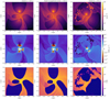 |
Fig. 2. Plane-parallel cuts (y = 0) of fluid quantities for different models. Left and middle columns: Model II without (βw = ∞) and with magnetized winds (βw = 100) 620 years into the simulation. Right column: Model III simulation 815 years into the simulation. Top row: Electron number density ne; Middle row: Accretion rate Ṁ; Bottom row: Temperature. |
In the simulation with higher metallicity of the stellar winds (Fig. 2, right column), the radiative cooling is more efficient, leading to the formation and ejection of cool, dense clumps. There is no sign of an accretion disk forming in our simulations; instead, accretion of matter happens primarily through close encounters of the stellar winds and the central black hole. This is true even for simulations with a disk-like distribution of stars (not shown).
Compared to the pure HD case, the Model II simulation with magnetic fields (Fig. 2, middle column) shows minimal differences, as magnetic fields do not appear to alter the global dynamics significantly.
3.2. Radial profiles
We present radial profiles of fluid quantities averaged over angles and time to better understand accretion dynamics. To do this, we first interpolate the data onto a spherical grid (r, θ, φ) logarithmically spaced in radius r, where the polar θ-axis is aligned with the z-axis of the simulation. Then we define the time (from tmin to tmax) and angle average of a quantity A as
 (4)
(4)
Figure 3a shows the radial dependence of the angle and time-averaged electron number density for our five simulations. In the outer region of the domain (r > 10−3 pc), the profiles are nearly identical. Closer to the IMBH, Models I and II generally follow a density scaling of ne ∝ r−1, whereas Model III exhibits a steeper density increase toward the system’s center. Figure 3b shows the radial dependence of the accretion rate,  . Positive values indicate outflow, while negative values correspond to inflow. The accretion rate profiles are similar across all scenarios, except in the region occupied by stellar winds due to their dynamic interaction. The system is predominantly outflow-driven, with the outflow rate (∼10−5 M⊙ yr−1) being approximately three orders of magnitude greater than the inflow rate at the simulation’s inner boundary (∼10−8 M⊙ yr−1). Assuming the accretion rate scales with the radius of the inner boundary of the simulation as
 (5)
(5)
which is appropriate for an r−1 scaling of density (Ressler et al. 2018; Guo et al. 2023; Xu 2023), extrapolating to the event horizon of a central black hole with mass M• = 3 × 10⁴ M⊙ yields an estimated accretion rate  .
.
Figures 3c and 3d present the radial profiles of radial velocity, vr, and temperature, T, respectively, demonstrating that these quantities are largely unaffected by the stellar wind configuration (at least for our assumption of circular orbits). In the inner region (r ≲ 10−3 pc), the temperature radial profile is similar to that of the density, T ∝ r−1, as expected for an approximately virial temperature. The temperature gradually decreases to ∼106 K at the outer domain boundary. The magnetized stellar wind simulation with βw = 100 is a minor outlier from these trends. Magnetic fields partially slow the outflow, so the winds reach slightly lower radial velocities. Dissipation of magnetic fields also contributes additional heating, leading to marginally higher temperatures.
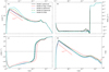 |
Fig. 3. Time and angle-averaged quantities in our simulations as a function of distance from the black hole, r. The different lines denote the different configurations of the simulation. (a) Density in the units of electron number density; (b) Accretion rate Ṁ; (c) Radial velocity of the gas vr; (d) Temperature of the gas. For the density and temperature radial profiles, a line representing ∝r−1 is also plotted for reference, highlighting the approximate power law in both quantities in the inner regions of the simulations. |
3.3. Angular momentum and magnetic effects
Figure 4 plots radial profiles of the time and angle-averaged specific angular momentum, l = r × v, where r and v are the position and velocity vectors, respectively, for both the magnitude of the average and the average of the magnitude scaled to the Keplerian specific angular momentum,  . These curves show that individual gas elements injected into the domain by the stellar winds generally have a super-Keplerian amount of angular momentum, meaning they tend to move outward in radius. On the other hand, the net angular momentum is relatively low in comparison because there is a significant amount of cancellation due to the lack of a consistent direction for the angular momentum. This is true even for the Model III disk-like stellar configuration, primarily because the wind speeds are higher than the orbital speeds. For distances from the black hole within the feeding region, fluid elements tend to have sub-Keplerian angular momentum (⟨|l|⟩ ∼ 0.3–0.4 lkep for the hydrodynamic simulations), implying that only the lowest angular momentum gas from the stellar winds falls inward. Since the wind speeds are relatively large, this gas corresponds with either low-impact parameter trajectories (i.e., gas blown almost directly at the black hole) or gas that loses its angular momentum through wind-wind shocks. Again, in this region, the magnitude of the net angular momentum is much lower than the average magnitude |⟨l⟩| ≲ 0.07 lkep, implying the lack of coherent accretion structure. The simulation with magnetic fields has the lowest ⟨|l|⟩, ≲0.2lkep, because magnetic forces tend to slow the gas.
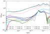 |
Fig. 4. Time and angle-averaged absolute value of the specific angular momentum ⟨|l|⟩ (dashed lines) as well as the absolute value of the average |⟨l⟩| (solid lines) normalized by the Keplerian value, lKep, as a function of distance from the black hole, r. |
Finally, for the magnetized wind simulation, Fig. 5 presents angle and time-averaged radial profiles of plasma beta (β = 2P/B2) for different averaging methods: ⟨β⟩ (solid line), ⟨P⟩ρ/⟨B2/2⟩ρ (dashed line), and  (dotted line), where we include the gas ram pressure along with the thermal pressure. Of these three curves,
  best represents the relative strength of magnetic energy/pressure relative to purely hydrodynamic energy/pressure. We find that
  for all radii implies that hydrodynamic forces dominate over magnetic ones. This is consistent with the radial profiles shown in Fig. 3, where the MHD simulation shows only moderate differences with the hydrodynamic simulations. ⟨P⟩ρ/⟨B2/2⟩ρ is generally lower than
  because the ram pressure is always significant when compared with the thermal pressure. In the region containing the stellar winds (r ∼ 10−3pc–10−2pc), ⟨P⟩ρ/⟨B2/2⟩ρ is particularly low (∼1–3) compared to
  because most of the hydrodynamical energy is contained in the kinetic energy of the winds, which have low thermal pressure.
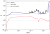 |
Fig. 5. Time and angle-averaged value of plasma β as a function of distance from the black hole, r, for the Model II simulation with magnetized winds using βw = 100. Different lines denote average ⟨β⟩ (solid line), density-weighted average ⟨β⟩ρ (dashed line), and |
4. Connection to observations
4.1. X-ray surface brightness density
To evaluate the detectability of the IMBH embedded within the cluster, we calculated the X-ray surface brightness density, SX. We used Model II spherical as our fiducial model, since the wind chemical composition here best aligns with the realistic expectation, and we see from Figs. 2–4 that all models are qualitatively similar. First, we used SPEX as described in Sect. 2.1 to calculate the cooling function, Λ, except we consider only the contributions from frequencies corresponding to the Chandra merged hard-band (2 − 7 keV) (Evans et al. 2010), denoting this as ΛX. Then we transform our simulation data to cylindrical coordinates (s, z, φ, with z being the line of sight) and integrate along the line of sight to obtain
 (6)
(6)
where zmax is one-half of the box length of the simulation. Figure 6 presents two snapshots of SX. The left panel corresponds to 650 years into the Model II spherical simulation, while the right panel depicts 830 years into the Model III spherical simulation, shortly after the timeframes shown in Fig. 1. At specific moments, emission from near the black hole becomes visible in the X-ray band (Fig. 6, left panel); however, the emission is typically dominated by the colliding stellar winds, rendering the black hole undetectable for most of the simulation (Fig. 6, right panel). Even when visible, the X-ray surface brightness at the location of the black hole remains lower than that of the surrounding winds.
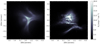 |
Fig. 6. Predicted intrinsic X-ray surface brightness density SX computed from our simulations scaled to Galactic center distance. Left: 650 years into the Model II spherical simulation. Right: 830 years into the Model III spherical simulation. The black hole is visible in the center of the left panel; however, the colliding winds dominate the X-ray emission and, most of the time, make the black hole undetectable (as seen in the right panel). |
Additionally, we roughly estimate the quiescent, thermal spectral energy distribution (SED) of the near-horizon flow (i.e., the flow within the inner boundary not modeled by our simulation) using the numerical prescription for an advection-dominated accretion flow (ADAF) using the formalism of Mahadevan (1997) presented in Pesce et al. (2021). Based on the black hole mass M•, accretion rate Ṁ, radiative efficiency η, plasma-β parameter, viscosity parameter α, power-law index for the mass accretion rate as a function of radius s, fraction of viscously dissipated energy that is advected f, and fraction of viscous heating that goes directly to the electrons δ (for numerical values see Pesce et al. 2021, Table 3), this one-zone model accounts for synchrotron, bremsstrahlung, and inverse Compton radiation. Figure 7 displays this SED, calculated using the time-averaged accretion rate extrapolated to the event horizon in the Model II spherical simulation in terms of the Eddington ratio λEdd, defined as
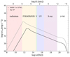 |
Fig. 7. Spectral energy distribution for the accretion flow near the IMBH at the center of the stellar association calculated using a simple ADAF model with a numerical prescription described in Pesce et al. (2021). The input for the model is the time-averaged accretion rate extrapolated to the event horizon of the IMBH (Ṁ = 2.1 × 10⁻¹⁰ M⊙ yr−1) and the associated Eddington ratio (λEdd = 3.168 × 10⁻⁷). For comparison, we also show an SED for Sgr A* calculated with the same model using Ṁ = 2.1 × 10⁻⁸ M⊙ yr−1 and Eddington ratio λEdd = 2.258 × 10⁻⁷. |
 (7)
(7)
where η is the radiative efficiency (assumed to be 0.1) and σT is the Thomson cross-section. We highlight specific spectral bands and include an approximate Sgr A* SED calculated using the same model for a typical accretion rate of 2 × 10⁻⁸ M⊙ yr−1, corresponding to an Eddington ratio of λEdd = 2.25 × 10⁻⁷ (Marrone et al. 2007). Compared to Sgr A*, the IMBH’s radiative flux is roughly three orders of magnitude lower across the spectrum, with its peak slightly shifted from the far-infrared (FIR) to the mid-infrared (MIR).
To estimate the relative contributions of the IMBH near-horizon emission and stellar wind collisions to the X-ray luminosity, we computed an IMBH ADAF spectrum every 5 years of the simulation time and integrate over the X-ray band. We then compare this to the total X-ray luminosity, LX, computed from the simulation by integrating
 (8)
(8)
where rin is the radius of the inner boundary. Figure 8 illustrates the time evolution of the X-ray luminosity for the ADAF SED model associated with the IMBH and the large-scale emission from the IMBH, computed from Eq. (6) integrated over the central 10−4 pc encompassing the black hole (left), the large-scale flow modeled by our simulations, computed from Eq. (8) integrated over the whole domain (middle), and all lines combined on the same plot (right). The luminosity produced by the large-scale flow is approximately two orders of magnitude greater than the ADAF luminosity and the large-scale emission associated with the IMBH, reaffirming that stellar wind collisions dominate the X-ray spectrum.
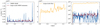 |
Fig. 8. Time evolution of the integrated X-ray luminosity computed from the Model II simulation. Left: X-ray luminosity of a near-horizon ADAF model for the IMBH as well as well as the large-scale emission from the vicinity of the IMBH. Middle: X-ray luminosity of the large-scale flow. Right: IMBH ADAF, IMBH large-scale flow, and total X-ray luminosity combined; we note that the vertical scale is logarithmic. |
4.2. X-ray data analysis
To compare the simulated X-ray signal with actual X-ray data of the IRS 13E source, we used archival observations obtained by the Chandra X-ray Observatory. We analyzed 128 non-grating ACIS-S and ACIS-I Chandra Observational IDs (OBSIDs) with Sgr A* in the aim-point spanning almost 25 years. All observations are reprocessed using the chandra_repro script (CIAO 4.17; Fruscione et al. 2006) and the latest calibration files (CALDB 4.11.6).
We performed relative astrometric corrections using the fine_astro script to obtain the best possible match between observations. As a reference, we used the OBSID 11843, which provides long enough exposure (78 ks) with a minimum of bright transient sources close to the chip aim-point, which would complicate source-matching with other OBSIDs. Before merging all OBSIDs, we further omit observations containing very bright transient sources in the vicinity of IRS 13E that would contaminate its signal, and we end up with 112 observations with a total cleaned exposure time of ≈3.6 Ms (≈2 Ms for ACIS-S and ≈1.6 for ACIS-I).
When reprocessing the individual OBSIDs using the chandra_repro script, we used the default value for the pix_adj parameter (pix_adj=EDSER), which allows us to leverage the subpixel Chandra resolution. We then produce a merged hard-band (2 − 7 keV) image binned to a pixel size of ≈0.125 arcsec. This allows us to study the morphology of the X-ray source corresponding to IRS 13E.
The simulated mock Chandra image obtained by scaling the X-ray surface brightness map (Fig. 6) to a distance of 8 kpc and then using the SOXS package (ZuHone et al. 2023) to simulate a mock Chandra ACIS-S1 observation with 3.6 Ms exposure time. Based on the simulated event file, we then produce a hard-band image binned to match the pixel size of the real Chandra subpixel image (≈0.125 arcsec). We compared the subpixel Chandra image to the simulated image at t = 50 yr in Fig. 9. We chose this time arbitrarily, since the simulated image does not change much throughout the simulation, with only the emission centroid moving slightly depending on where the winds collide the most. Given the uncertainties in the stellar wind parameters, the qualitative agreement between the Chandra image and the mock image from our simulation is quite good except for minor differences. In Appendix C and in particular in Fig. C1, we compared the surface-brightness profiles between the observed image and the simulated one. The simulation produces a slightly more spherical distribution of X-ray luminosity, which we demonstrate by evaluating the asymmetry parameter (A = 0.13 for the simulated image vs. A = 0.21 for the observed one). This result is not surprising because we assumed that all the stars were on spherical orbits. More importantly, the Chandra image also contains an extended, diffuse emission outside the brighter core. In addition, there are additional background/foreground X-ray point sources in the IRS 13E field. Our simulations do not contain any more distant sources, and the simulated image is thus based entirely on the six stars listed in Table 3 that orbit the IMBH. However, apart from the differences in the tails of the X-ray surface-brightness profile, both profiles are qualitatively consistent with the uncertainties. They closely follow and are slightly wider than the Chandra point-spread function (PSF). From a quantitative point of view, the total flux/luminosity of IRS 13E and the simulated cluster differ significantly, with the simulated cluster being more luminous by an order of magnitude. The agreement could be reached, for example, by fine-tuning the WR stars’ mass-loss rates and wind velocities within the uncertainties. Since we did not seek an exact model for IRS 13E at this point, we will explore the parameter space of the cluster in relation to IRS 13E in the upcoming study in more detail.
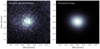 |
Fig. 9. Left: Merged subpixel Chandra image obtained by combining 112 non-grating ACIS-S and ACIS-I observations with a total cleaned exposure time of almost 3.6 Ms. Right: Mock Chandra ACIS-S image obtained using the SOXS simulator based on a Model II spherical simulation snapshot at 50 years. |
4.3. Accretion rate and X-ray variability
In addition to the time-averaged and angle-integrated radial profiles of the accretion rate (Fig. 3), we also analyze the time variability. In particular, we focus on the accretion rate at the inner boundary of the computational domain extrapolated to the event horizon using Eq. (5), shown in the top left and top right panels of Fig. 10 for the spherical and disk-like stellar distributions. The variability is quite pronounced, with spikes in accretion rate up to an order of magnitude, i.e. from Ṁ∙ ∼ 10−10 M⊙ yr−1 up to Ṁ∙ ∼ 10−9 M⊙ yr−1 on a timescale of ∼20 years.
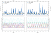 |
Fig. 10. Temporal evolution of the mass inflow rate Ṁ (top row) and mutual distances between the shortest-period star E4 and other stars expressed in au (bottom row) for the isotropic spherical (left column) and disk-like (right column) stellar configurations. The minimum distances for each pair are represented via solid horizontal lines of corresponding color. In both configurations, periodic approaches between the closest star, E4, and all other stars are responsible for the periodic spikes in the inflow rate, with the shortest separations reaching ∼1000 au. |
In order to isolate candidate periodicities in the accretion rate, we computed Lomb–Scargle (LS) periodograms (Lomb 1976; Scargle 1982), as detailed in Appendix B. Our simulations typically span around 2000 years, and we sample every 5 years, meaning that we can identify periodic signals in the time range from 10 to 1000 years. For the accretion rate in spherically distributed stellar systems, we detect a prominent periodicity peak at ∼110 years for both low and high metallicity. In addition, peaks at ∼200 years, ∼55 years, and ∼70 years are also pronounced, as shown in Figs. B1–B3 (left panels). For the disk-like stellar configuration, the most prominent peak is at ∼186 years, followed by peaks at ∼217 and ∼100 years, respectively, as shown in Fig. B4 (left panel).
These detected periodicities induced close encounters between stars, during which their strong stellar winds are compressed and shocked. The most shocked, denser gas flows out of the system while a small fraction accretes onto the black hole. In Appendix A, there is a comprehensive overview of the approaches of the stellar pairs, including minimum, mean, and maximum distances (in AU) and the associated recurrence timescales (in years). The most pronounced periods are associated with the star E4, which has the most compact orbit (at a distance of 4.06 mpc). For the adopted spherical setup of stars, the closest approaches between stars E4 and E5.1 take place every 108 years, which is consistent with the most prominent periodicity peak in the inflow rate, compare Fig. 10 (left column) and Figs. B1–B3. On the other hand, for the disk-like setup, the approaches between the same stars (E4 and E5.1) take place every 198 years, which is again consistent with the broader peak around 186–217 years in the periodogram (Fig. B4; compare with Fig. 10, right column). The closest approaches between star E4 and other stars take place with comparable periods of ∼100 − 200 years (see Tables A.1 and A.2), which further affects the mass inflow rate; specific inflow peaks are strengthened or prolonged when the stellar approaches take place almost simultaneously. In addition, occasional rare approaches on the scale of ∼100 − 200 AU among other stars can further significantly modulate the inflow rate at some epochs. Altogether, this results in multiple periodicity peaks for all the runs in the periodograms.
In Appendix B, we also construct power spectral densities (PSDs) of the accretion rates (shown in the right panels of Figs. B1 and B4). Overall, except for the presence of peaks due to the periodocities already discussed (at ∼100 and 200 years), the PSD profiles are consistent with a simple power law function with the mean slope of ∼ − 0.60, which implies the presence of underlying stochastic variability.
Finally, we computed Lomb–Scargle periodograms (Fig. 11) and PSDs (Fig. 12) for the X-ray light curves presented in Sect. 4.2. Because the magnitude and the spectral shape of the X-ray portion of the ADAF model’s SED (Fig. 7) depend on the variable accretion rate, the time-variability is not one-to-one with the accretion rate. The Lomb–Scargle periodograms of the ADAF models display significant peaks at ∼210 years and ∼54 years. In contrast, the peak around ∼110 years appears to be suppressed compared to the periodogram of the accretion rate in Fig. B1. On the other hand, the total X-ray luminosity, which dominated the shocked stellar winds, has a significant periodic component at ∼104 years, corresponding to the periods of close approaches among the stellar pairs E4–E1 and E4–E5.1. In terms of power, the PSD for the ADAF model is significantly flatter than the PSD for the whole cluster (with power-law slopes of ∼ − 0.53 vs. ∼ − 1.41). This is consistent with the fact that there is more short-term variability on timescales of < 100 years in the region closer to the inner boundary of the simulation than on larger scales of the cluster.
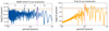 |
Fig. 11. Lomb–Scargle periodograms of the X-ray light curves computed from the simulations. Left: LS periodogram of the X-ray light curve produced by the near-horizon flow around the IMBH as calculated from an ADAF model. The highest peak is at ∼210 years, while other prominent peaks are at ∼54 and ∼83 years. The dotted horizontal lines mark inferred confidence levels based on 10 000 bootstrap realizations. Right: LS periodogram of the total X-ray luminosity exhibits the highest peak at ∼104 years. Other prominent peaks are at ∼202, ∼271, ∼55, and ∼74 years. The dotted horizontal lines stand for the confidence levels, as in the left panel. |
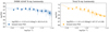 |
Fig. 12. Power spectral densities of the X-ray variability of the compact stellar cluster with an IMBH. Left: PSD of the X-ray light curve produced by the near-horizon flow around the IMBH as calculated from an ADAF model, which has a flat power-law slope of ∼ − 0.53. Right: PSD of the total X-ray light curve, which exhibits a steeper power-law slope of ∼ − 1.41. The points represent mean PSD values within the ten regular logarithmic bins in frequency, while the error bars represent standard deviations in these bins. We fit the power-law functions to these binned PSD values for consistency. In both panels, the extents of the logarithms of PSDs and frequencies are kept the same for consistency and easier comparison. |
We also characterize the intrinsic IMBH ADAF variability in terms of the fractional variability (Nandra et al. 1997; Rodríguez-Pascual et al. 1997; Martínez-Aldama et al. 2019),
 (9)
(9)
where σ2 is the variance of the luminosity, Δ2 is the mean square uncertainty associated with individual luminosities Li, and  is the mean luminosity. Assuming one percent relative uncertainty for both the IMBH ADAF and the total (cluster) luminosities (see Fig. 8 left and middle panels), we obtain Fvar ≃ 213% for the IMBH’s ADAF X-ray luminosity, while we infer Fvar ≃ 20% for the X-ray luminosity of the whole cluster (for a luminosity uncertainty of 10%, Fvar ≃ 212% and Fvar ≃ 17% for the IMBH’s ADAF and the total luminosities, respectively). Hence, the cluster X-ray emission, whose variability is mild, masks a much more vigorous X-ray emission of the IMBH ADAF. This is also consistent with the flatter power spectral density of the ADAF variability (∝f−0.5) in comparison with the PSD of the total luminosity (∝f−1.4), see Fig. 12. The quasiperiodic X-ray spikes associated with the IMBH with the typical timescale of ∼100 years are reminiscent of order-of-magnitude quasiperiodic X-ray eruptions (QPEs) detected for several both active and quiescent galactic nuclei (Miniutti et al. 2019; Arcodia et al. 2021; Suková et al. 2024). However, in contrast, QPEs take place on timescales five orders of magnitude smaller, and the QPE X-ray properties are consistent with being associated with the soft thermal X-ray emission. Still, in future work, it is worth considering a compact association of wind-blowing stars orbiting around the massive black hole in a galactic nucleus as a potential model to address some of the QPE sources. Such a simulation would have to be a scaled-down version of the MHD simulations presented in this work with the characteristic stellar orbit radius of rQPE = rIRS13(PQPE/PIRS13)2/3 ∼ 2 × 10⁻⁶ (rIRS13/4 × 10−3 pc)(PQPE/10 hours)2/3(PIRS13/100 years)−2/3pc for M = 3 × 10⁴ M⊙ (IMBH), which corresponds to rQPE ∼ 5.4 × 10⁻⁶ pc ∼ 111(PQPE/10 hours)2/3(M/106 M⊙)−2/3 gravitational radii for the M = 106 M⊙ supermassive black hole.
5. Discussion
5.1. IMBH accretion fueled by stellar winds
Understanding accretion onto IMBHs in wind-fed systems is crucial for understanding their growth and observational signatures. In the compact WR stellar cluster scenario studied here, the winds create an unstructured inflow that affects accretion efficiency and detectability in X-rays and other wavelengths. As shown in Fig. 1, the interaction of these winds results in a turbulent, inhomogeneous flow with dense filaments and outflow channels. Furthermore, only about 10−5 of the injected mass reaches the black hole. This stark disparity highlights that only a tiny fraction of the available wind material is captured. Consequently, the black hole is unlikely to experience significant growth in mass from stellar winds alone. The accretion rates in our models are several orders of magnitude smaller than would be expected if the IMBH fed a dense gas disk or a continuous gas inflow (e.g., Poutanen et al. 2013). This implies that other processes – such as external gas infall from the larger environment, tidal disruptions of stars, or mergers with compact objects – would be needed for the IMBH to increase its mass substantially.
The accretion process is highly intermittent and variable, primarily driven by the orbital motions of the stars: periodic close WR-WR and WR-IMBH passages induce spikes in the inflow rate (see Fig. 10). These findings illustrate that wind-wind interactions dominate the gas dynamics, which is comprised almost entirely of unbound material. Instead, the resulting flow structure is largely outflow-dominated, which can further limit the amount of infalling gas. In summary, wind-fed accretion in this environment is a fundamentally chaotic process markedly different from the orderly disk accretion scenarios often considered for black hole growth.
Our simulations identify several physical factors that collectively limit the accretion efficiency in this wind-fed system. First, the high velocity of the WR winds (on the order of vw ∼ 1000 km s−1; Krabbe et al. 1995) means that much of the ejected gas moves faster than the escape speed defined with respect to the IMBH (the escape speed at r = 0.01 pc is 165 km s−1). The radial profile of accretion rate (Fig. 3) confirms that outflows dominate, indicating that most of the wind material is expelled before it can be captured. Shock heating from wind–wind collisions keeps the gas hot and turbulent, further impeding any steady inflow.
The IMBH’s radiative output would be pretty low with such a meager feeding rate. Assuming an advection-dominated (radiatively inefficient) accretion flow, we predict a quiescent X-ray luminosity of only LX ∼ 1032 erg s−1, with short-lived bursts up to ∼1033 erg s−1 during quasi-periodic accretion spikes, many orders of magnitude below the Eddington luminosity for a 3 × 10⁴ M⊙ black hole (LEdd ∼ 1042–1043 erg s−1).
The efficiency of radiative cooling – which depends on the wind’s metal content – strongly influences the morphology of the flow. In the high-metallicity case (Z = 0.4, representative of WC8–9 type WR stars; Crowther 2007), cooling instabilities induce the formation of dense clumps via thin-shell shocks at wind–wind collision interfaces (e.g., Stevens et al. 1992; Calderón et al. 2025). Nevertheless, as noted above, these clumps do not substantially boost accretion. By contrast, in the lower-metallicity case, the winds stay hotter and smoother, and the added thermal pressure further inhibits gas from falling inward.
The specific angular momentum of the inflowing gas (Fig. 4) gives further insight into the structure and behavior of the accretion flow. Because the wind speeds are so high relative to the orbital speeds of the stars, most gas is injected into the domain with super-Keplerian angular momentum pointing in quasi-random directions. As a result, only the gas that is either directed very close to the black hole that loses its angular momentum through wind-wind shocks can accrete. In the inner domain, this leads to a low angular momentum (in terms of individual fluid elements and the net average) accretion flow without a coherent structure.
Magnetic fields present in the stellar winds introduce additional physical effects. In the model with moderately magnetized winds (βw = 100), we observe that magnetic pressure slows the inflow and enhances turbulence. Magnetic dissipation converts some field energy into heat, raising the gas pressure and counteracting a portion of the radiative cooling. Although including magnetic fields does not dramatically change the global accretion rate in our simulations, it alters the geometry of outflows. It suggests that even stronger wind magnetization could further inhibit accretion. β profiles shown in Fig. 5 demonstrate that the combined thermal and ram pressure of the gas dominates the balance – evidenced by β ≫ 1 at virtually all radii – meaning that the overall inflow–outflow structure is shaped primarily by hydrodynamic forces.
Beyond accretion, the IMBH’s presence could influence the cluster’s overall dynamics. The kinetic energy imparted by the stellar winds and their interaction with the IMBH drives turbulence, potentially limiting the retention of cold gas in the cluster. Similar effects have been seen in AGN feedback studies involving observations, models, or both (e.g., Zubovas & King 2012; King & Pounds 2015; Wylezalek & Zakamska 2016), where accretion flow-driven outflows can heat and expel surrounding material. This turbulence and gas expulsion may impact the long-term evolution of the cluster, affecting star formation and modifying the density profile. However, these effects are not solely dependent on the presence of IMBH. Future studies incorporating stellar evolution and external gas supply mechanisms will be crucial for understanding the full impact of IMBHs in such environments.
In summary, wind-fed accretion onto an IMBH in a dense stellar cluster is inefficient. The high-velocity winds effectively starve the black hole, keeping its accretion luminosity low. Consequently, the IMBH would remain practically invisible against the bright background of colliding-wind X-ray emission from the cluster (as discussed later), even though its presence can still perturb the surrounding medium through gravity and outflows.
5.2. Comparison with other wind-fed accretion regimes
Wind-fed accretion has been most extensively studied in the context of Sgr A* – the supermassive black hole at the Galactic center – which feeds the winds of nearby massive stars (e.g., Cuadra et al. 2008; Ressler et al. 2018, 2019b; Calderón et al. 2020b, 2025). Our work is the first to explore a similar wind-fed accretion scenario for an IMBH embedded in a compact star cluster. Comparing the two cases provides insight into how differences in black hole mass, stellar cluster size, wind properties, and cooling processes affect accretion dynamics and efficiency.
The physical scale and environment are key distinctions between Sgr A* and our IMBH scenario. Sgr A* (M• ≈ 4 × 10⁶ M⊙) lies in the Galactic nucleus, surrounded by a relatively extended cluster of OB-spectral type and WR stars spread over a region of a few tenths of a parsec. In contrast, our simulations consider a much smaller black hole (M• = 3 × 10⁴ M⊙) embedded in a very compact cluster (with radial extent on the order of 0.1 pc) of only a handful of WR stars. Therefore, the stellar density in the IMBH’s immediate vicinity is much higher in our scenario. On the other hand, the ratio between the gravitational capture radius of the IMBH and the scale of the cluster is comparable to that of the SMBH in the Galactic center.
Sgr A* and the simulated IMBH exhibit extremely low accretion efficiencies in their wind-fed modes. HD simulations of Sgr A*’s environment have shown that only a small fraction of the stellar wind material (of order 10−3) captured the SMBH, while the rest is blown away by outflows (Cuadra et al. 2008; Ressler et al. 2018). In our IMBH case, the captured fraction is even smaller, on the order of 10−5. In absolute terms, the time-averaged accretion rate for Sgr A* is estimated to be ∼10−9–10−7 M⊙ yr−1, whereas in our simulations it is ∼10−10 M⊙ yr−1. The outcome is qualitatively similar despite the two-order-of-magnitude difference in black hole mass. In both systems, most available wind mass is expelled, and only a small fraction feeds the black hole.
In both cases, the primary factor driving accretion inefficiency is the high wind velocity relative to the gravitational capture threshold. For an IMBH of mass M• = 3 × 10⁴ M⊙, the Bondi radius, which represents the scale at which gravitational influence becomes significant, is
 (10)
(10)
where  is the sound speed of the gas. Assuming an adiabatic index of γ = 5/3 and a resulting kBT = 3/16 mpvw2 for strongly shocked gas, we can rewrite the Bondi radius in terms of wind speed vw as
 (11)
(11)
This is one order of magnitude smaller than the cluster scale and consistent with the inflow-outflow boundary in the velocity and accretion rate profiles shown in Fig. 3. Most wind material escapes before experiencing significant gravitational influence. In comparison, even though Sgr A*’s deeper gravitational potential results in a larger RB ∼ 0.05 pc, stars in the inner parsec of the Galactic center are generally further out (∼0.2 pc). The ratio between the Bondi radius and star distances in both systems is comparable, and the high wind speeds relative to the escape velocity lead to substantial mass loss in outflows rather than sustained accretion.
In both systems, radiative cooling can lead to the formation of clumpy, filamentary structures in the accretion flow, depending on the gas composition. In the Galactic center, these clumps can be bound and can therefore collect into an accretion disk and substantially raise the long-term accretion rate (e.g., Calderón et al. 2020b, 2025). In contrast, in our IMBH simulations, the dense clumps only momentarily increase local densities but are quickly disrupted or ejected, yielding no significant enhancement of accretion or disk formation.
Finally, while both observations of Sgr A* and our IMBH model display relatively low quiescent X-ray luminosities (LX ∼ 1033 erg s−1 for Sgr A* and ∼1032 erg s−1 for the IMBH), they also show evidence of intermittent, episodic accretion events. Sgr A* exhibits frequent, daily flares in X-rays and near-infrared domains as well as at longer wavelengths (Baganoff et al. 2001; Porquet et al. 2003; Yusef-Zadeh et al. 2006; Genzel et al. 2010; Eckart et al. 2012, 2017; Witzel et al. 2021; von Fellenberg et al. 2025), thought to be triggered by sudden increases in accretion or magnetic reconnection events in the near-horizon flow that accelerate electrons to nonthermal energies (e.g., Dexter et al. 2020; Porth et al. 2021; Ripperda et al. 2022). Our simulations also observe short-lived accretion spikes when individual stars pass particularly close to each other and their wind collisions funnel gas inward. However, these bursts are much weaker relative to the quiescent X-ray emisison (LX ≲ 1032–1033 erg s−1) than the observed Sgr A* flares (the largest being LX ≲ 3 − 4 × 1035 erg s−1, 160 times the quiescent level Porquet et al. 2003), since our simulations do not capture the relevant scales or non-ideal physics important for such larger flares, we cannot rule them out. In fact, since both systems are in the radiatively inefficient regime with many qualitatively similar features in their larger-scale flow, we posit that high-magnitude flares originating from the near-horizon flow around the IMBH are likely (though on comparatively shorter timescales).
5.3. Observability
Our findings suggest that detecting an embedded IMBH in a WR stellar cluster poses a major observational challenge because the radiation from the accreting IMBH overwhelmed the emission from the surrounding stellar winds (as shown by our synthetic X-ray images in Fig. 6). Throughout our simulations, most high-energy photons originate from wind–wind shock heating. This is true even when we account for the analytically predicted ADAF spectrum produced by the near-horizon flow (Figures 7 and 8), which results in an X-ray luminosity that is a factor of about 102-103 smaller than that resulting from the wind-wind collisions. In absolute terms, the IMBH’s X-ray luminosity in our models (of order 1032 erg s−1) is extremely low – consistent with the nondetections and upper limits for IMBH candidates in similar environments (e.g., Chilingarian et al. 2018; Wang et al. 2020) – whereas the total diffuse X-ray luminosity of the cluster (from the stellar winds) is about 1034-1035 erg s−1.
Therefore, the primary difficulty for observers is one of contrast: disentangling the IMBH’s fainter radiative signal from the luminous stellar wind environment. In our scenario, the black hole would be effectively “lost in the glare” of the cluster’s collective emission, emphasizing the need for sensitive, high-resolution observations to find an IMBH’s steady glow amid the cluster’s background. On the other hand, our simulations do not capture the physics and scales required for Sgr A*-like X-ray and infrared flares, meaning that there could still be strong transient signals. Evaluating this possibility is an important task for future work that includes such physics.
Future X-ray and radio missions will provide higher sensitivity for detecting these objects. The proposed Lynx X-ray Observatory (Gaskin et al. 2019) will feature an angular resolution of ∼0.5 arcseconds, comparable to Chandra X-ray Observatory, but with significantly improved sensitivity. This could enable the detection of faint persistent X-ray sources in dense stellar environments where IMBHs are suspected to reside. Given that the primary observational challenge is distinguishing the IMBH’s weak, point-like accretion signature from the surrounding diffuse stellar-wind emission, Lynx’s superior imaging and spectroscopic capabilities could be critical for resolving such sources. Similarly, the Advanced X-ray Imaging Satellite (AXIS) (Reynolds et al. 2023) is designed to provide high angular resolution X-ray imaging with a resolution of about 1.5 arcseconds across a wide field of view. Scheduled for launch in 2032, AXIS aims to study high-energy phenomena in the universe, including detecting faint X-ray sources in dense stellar environments. Its rapid response capabilities to transient events and improved sensitivity make it a promising tool for identifying IMBHs. Looking further ahead, X-ray interferometry holds exciting potential for the future of high-resolution X-ray astronomy. By overcoming the diffraction limits of traditional telescopes, space-based X-ray interferometers could achieve microarcsecond angular resolution, making it possible to directly image IMBH environments and distinguish them from surrounding stellar activity (Uttley et al. 2021). Although still in an early conceptual phase, continued advancements in this technology could one day provide an unprecedented tool for confirming and characterizing IMBHs in dense stellar clusters.
Beyond X-rays, radio observations offer complementary constraints. IMBHs accreting in a radiatively inefficient mode may exhibit faint synchrotron radio emission, analogous to low-luminosity AGN (Mezcua et al. 2018). Upcoming facilities such as the Square Kilometer Array (SKA) (Dewdney et al. 2009) could help probe this parameter space, particularly in nearby dense stellar clusters where IMBH candidates are suspected to reside. Furthermore, from the SED shown in Fig. 7 and after applying the extinction curve from Fritz et al. (2011), IRS 13E’s putative IMBH should exhibit radiative flux of 0.5–1.2 mJy at 19 μm. Assuming that the 25–80% FIR variability of Sgr A*’s peak thermal emission (von Fellenberg et al. 2018; Wielgus et al. 2022) is typical for low-luminosity accretion flows, this would result in ∼0.1–1 mJy mid-IR variability for the IRS 13E IMBH’s peak thermal emission, which should be detectable with JWST/MIRI (Wright et al. 2023).
Given the limitations of the current observational missions, future searches for IMBHs in stellar clusters should focus on:
-
High-sensitivity X-ray imaging with subarcsecond resolution to detect weak, persistent accretion signatures.
-
Time-domain surveys to search for transient accretion events or variability in cluster-integrated X-ray emission.
-
Deep radio observations to constrain possible synchrotron emission from IMBHs accreting in a radiatively inefficient mode.
-
Multiwavelength approaches that combine NIR, X-ray, and radio data to build a comprehensive observational profile.
Overall, while our simulations reinforce that an IMBH in a compact stellar cluster would be extremely difficult to detect with current instruments, the next generation of observatories coupled with coordinated multiwavelength efforts may provide the necessary sensitivity and resolution to finally uncover these elusive objects.
6. Conclusions
We conducted 3D MHD simulations to study wind-fed accretion onto an IMBH of mass Ṁ∙ = 3 × 10⁴ M⊙ embedded in a compact stellar cluster of six WR stars. Using the grid-based code ATHENA++, we modeled the stellar winds (with wind velocities of vw ∼ 100 km s−1) and their interactions with the IMBH’s gravitational potential while varying the cluster’s stellar distribution, wind magnetization, and chemical composition.
From the simulations, we found that only 10−5 of the injected wind mass reaches the black hole. Wind-wind interactions dominate the dynamics, and the system is outflow-dominated. The gas follows a virial temperature profile, reaching T ∼ 108 K near the boundary, while high wind velocities exceed the escape speed, ensuring most gas remains unbound. In higher-metallicity environments, enhanced radiative cooling forms cool, dense clumps, but their transient nature and high velocities prevent efficient accretion. The inflowing gas remains well below the Keplerian angular momentum, favoring a quasi-Bondi-like, radial accretion mode. Magnetic fields slightly suppress outflows but do not significantly affect the net accretion rate.
Observationally, the system’s X-ray emission dominated wind-wind shocks, with total luminosities of LX ∼ 1034−1035 erg s−1, while the extrapolated near-horizon flow around the IMBH is much fainter at LX ∼ 1032 erg s−1. X-ray emission is wind-dominated, so IMBH signatures remain below current detection thresholds. Although weak, the X-ray emission of the near-horizon flow around the IMBH is highly variable with quasiperiodic flares recurring every ∼100 − 200 years due to the close passages of the nearest star with the surrounding stars.
These results suggest that IMBHs in dense stellar clusters grow slowly if fed solely by stellar winds. In this quiescent regime, they do not affect their surroundings significantly through feedback. Instead, wind-wind collisions due to the cluster stars influence the closest environment through kinetic feedback. Feedback from the IMBH could be enhanced for example by the tidal disruption of one of the cluster stars or the accretion of an additional external gas reservoir. Future work should investigate these possibilities and study the long-term cluster evolution to better understand the detectability of IMBHs and their role in stellar dynamics.
Effective area corresponding to Cycle 22 was assumed.
Acknowledgments
We thank S. von Fellenberg for useful discussions. ML and TP have received support from the GAČR EXPRO grant no. GX21-13491X. MZ acknowledges the financial support of the GAČR Junior Star grant no. GM24-10599M. BR and SMR supported the Natural Sciences & Engineering Research Council of Canada (NSERC). BR supported the Canadian Space Agency (23JWGO2A01), and by a grant from the Simons Foundation (MP-SCMPS-00001470). BR acknowledges a guest researcher position at the Flatiron Institute, supported by the Simons Foundation. F.P. gratefully acknowledges the Collaborative Research Center 1601 funded by the Deutsche Forschungsgemeinschaft (DFG, German Research Foundation) – SFB 1601 [sub-project A3] – 500700252. The computational resources and services used in this work were partially provided by facilities supported by the VSC (Flemish Supercomputer Center), funded by the Research Foundation Flanders (FWO) and the Flemish Government – department EWI, and by Compute Ontario and the Digital Research Alliance of Canada (alliancecan.ca) compute allocation rrg-ripperda.
References
- Abbott, R., Abbott, T. D., Abraham, S., et al. 2020, ApJ, 900, L13 [NASA ADS] [CrossRef] [Google Scholar]
- Akiba, T., Naoz, S., & Madigan, A.-M. 2025, ApJ, 987, L27 [Google Scholar]
- Arcodia, R., Merloni, A., Nandra, K., et al. 2021, Nature, 592, 704 [NASA ADS] [CrossRef] [Google Scholar]
- Baganoff, F. K., Bautz, M. W., Brandt, W. N., et al. 2001, Nature, 413, 45 [Google Scholar]
- Bañares-Hernández, A., Calore, F., Martin Camalich, J., & Read, J. I. 2025, A&A, 693, A104 [NASA ADS] [CrossRef] [EDP Sciences] [Google Scholar]
- Banerjee, S., & Kroupa, P. 2011, ApJ, 741, L12 [NASA ADS] [CrossRef] [Google Scholar]
- Bartko, H., Martins, F., Fritz, T. K., et al. 2009, ApJ, 697, 1741 [Google Scholar]
- Begelman, M. C., Volonteri, M., & Rees, M. J. 2006, MNRAS, 370, 289 [NASA ADS] [CrossRef] [Google Scholar]
- Britzen, S., Zajaček, M., Gopal-Krishna, et al. 2023, ApJ, 951, 106 [CrossRef] [Google Scholar]
- Calderón, D., Cuadra, J., Russell, C. M. P., & Wang, Q. D. 2016, MNRAS, 455, 4388 [Google Scholar]
- Calderón, D., Cuadra, J., Schartmann, M., et al. 2020a, MNRAS, 493, 447 [Google Scholar]
- Calderón, D., Cuadra, J., Schartmann, M., Burkert, A., & Russell, C. M. P. 2020b, ApJ, 888, L2 [Google Scholar]
- Calderón, D., Cuadra, J., Russell, C. M. P., et al. 2025, A&A, 693, A180 [NASA ADS] [CrossRef] [EDP Sciences] [Google Scholar]
- Cao, C., Liu, F. K., Li, S., Chen, X., & Wang, K. 2025, ApJ, 982, L37 [Google Scholar]
- Čechura, J., & Hadrava, P. 2015, A&A, 575, A5 [Google Scholar]
- Čechura, J., Vrtilek, S. D., & Hadrava, P. 2015, MNRAS, 450, 2410 [CrossRef] [Google Scholar]
- Chatterjee, P., Hernquist, L., & Loeb, A. 2002a, Phys. Rev. Lett., 88, 121103 [NASA ADS] [CrossRef] [Google Scholar]
- Chatterjee, P., Hernquist, L., & Loeb, A. 2002b, ApJ, 572, 371 [NASA ADS] [CrossRef] [Google Scholar]
- Chilingarian, I. V., Katkov, I. Y., Zolotukhin, I. Y., et al. 2018, ApJ, 863, 1 [Google Scholar]
- Crowther, P. A. 2007, ARA&A, 45, 177 [Google Scholar]
- Cuadra, J., Nayakshin, S., Springel, V., & Di Matteo, T. 2005, MNRAS, 360, L55 [CrossRef] [Google Scholar]
- Cuadra, J., Nayakshin, S., Springel, V., & Di Matteo, T. 2006, MNRAS, 366, 358 [NASA ADS] [CrossRef] [Google Scholar]
- Cuadra, J., Nayakshin, S., Martins, F., et al. 2008, MNRAS, 383, 458 [NASA ADS] [CrossRef] [Google Scholar]
- Cuadra, J., Nayakshin, S., & Wang, Q. D. 2015, MNRAS, 450, 277 [CrossRef] [Google Scholar]
- Dewdney, P. E., Hall, P. J., Schilizzi, R. T., & Lazio, T. J. L. W. 2009, IEEE Proc., 97, 1482 [Google Scholar]
- Dexter, J., Tchekhovskoy, A., Jiménez-Rosales, A., et al. 2020, MNRAS, 497, 4999 [Google Scholar]
- Do, T., Lu, J. R., Ghez, A. M., et al. 2013, ApJ, 764, 154 [NASA ADS] [CrossRef] [Google Scholar]
- Eckart, A., García-Marín, M., Vogel, S. N., et al. 2012, A&A, 537, A52 [NASA ADS] [CrossRef] [EDP Sciences] [Google Scholar]
- Eckart, A., Hüttemann, A., Kiefer, C., et al. 2017, Found. Phys., 47, 553 [NASA ADS] [CrossRef] [Google Scholar]
- Eisenstein, D. J., & Loeb, A. 1995, ApJ, 443, 11 [NASA ADS] [CrossRef] [Google Scholar]
- Evans, I. N., Primini, F. A., Glotfelty, K. J., et al. 2010, ApJS, 189, 37 [NASA ADS] [CrossRef] [Google Scholar]
- Ferrarese, L., & Merritt, D. 2000, ApJ, 539, L9 [Google Scholar]
- Filippenko, A. V., & Ho, L. C. 2003, ApJ, 588, L13 [NASA ADS] [CrossRef] [Google Scholar]
- Fragione, G., Kocsis, B., Rasio, F. A., & Silk, J. 2022, ApJ, 927, 231 [NASA ADS] [CrossRef] [Google Scholar]
- Freitag, M., Gürkan, M. A., & Rasio, F. A. 2006, MNRAS, 368, 141 [NASA ADS] [Google Scholar]
- Fritz, T. K., Gillessen, S., Dodds-Eden, K., et al. 2010, ApJ, 721, 395 [Google Scholar]
- Fritz, T. K., Gillessen, S., Dodds-Eden, K., et al. 2011, ApJ, 737, 73 [Google Scholar]
- Fruscione, A., McDowell, J. C., Allen, G. E., et al. 2006, SPIE Conf. Ser., 6270, 62701V [Google Scholar]
- Fujii, M. S., Wang, L., Tanikawa, A., Hirai, Y., & Saitoh, T. R. 2024, Science, 384, 1488 [NASA ADS] [CrossRef] [Google Scholar]
- Gaskin, J. A., Swartz, D. A., Vikhlinin, A., et al. 2019, JATIS, 5, 021001 [NASA ADS] [Google Scholar]
- Gebhardt, K., Bender, R., Bower, G., et al. 2000, ApJ, 539, L13 [Google Scholar]
- Genzel, R., Eisenhauer, F., & Gillessen, S. 2010, Rev. Mod. Phys., 82, 3121 [Google Scholar]
- Giersz, M., Leigh, N., Hypki, A., Lützgendorf, N., & Askar, A. 2015, MNRAS, 454, 3150 [Google Scholar]
- Greene, J. E., Strader, J., & Ho, L. C. 2020, ARA&A, 58, 257 [Google Scholar]
- Gültekin, K., Miller, M. C., & Hamilton, D. P. 2004, ApJ, 616, 221 [Google Scholar]
- Guo, M., Stone, J. M., Kim, C.-G., & Quataert, E. 2023, ApJ, 946, 26 [NASA ADS] [CrossRef] [Google Scholar]
- Haas, J., Kroupa, P., Šubr, L., & Singhal, M. 2025, A&A, 695, L19 [NASA ADS] [CrossRef] [EDP Sciences] [Google Scholar]
- Häberle, M., Neumayer, N., Seth, A., et al. 2024, Nature, 631, 285 [CrossRef] [Google Scholar]
- Hadrava, P., & Čechura, J. 2012, A&A, 542, A42 [NASA ADS] [CrossRef] [EDP Sciences] [Google Scholar]
- Hansen, B. M. S., & Milosavljević, M. 2003, ApJ, 593, L77 [NASA ADS] [CrossRef] [Google Scholar]
- Hendrix, T., Keppens, R., van Marle, A. J., et al. 2016, MNRAS, 460, 3975 [NASA ADS] [CrossRef] [Google Scholar]
- Herald, J. E., Hillier, D. J., & Schulte-Ladbeck, R. E. 2001, ApJ, 548, 932 [Google Scholar]
- Hosseini, S. E., Eckart, A., Zajaček, M., et al. 2024, ApJ, 975, 261 [CrossRef] [Google Scholar]
- Hu, D., Zajaček, M., Werner, N., et al. 2024, MNRAS, 527, 1062 [Google Scholar]
- Jin, C. C., Li, D. Y., Jiang, N., et al. 2025, ArXiv e-prints [arXiv:2501.09580] [Google Scholar]
- Kaastra, J., Mewe, R., Nieuwenhuijzen, H., et al. 1996, UV and X-ray Spectroscopy of Astrophysical and Laboratory Plasmas [Google Scholar]
- Kee, N. D., Owocki, S., & ud-Doula, A. 2014, MNRAS, 438, 3557 [Google Scholar]
- King, A., & Pounds, K. 2015, ARA&A, 53, 115 [NASA ADS] [CrossRef] [Google Scholar]
- Kızıltan, B., Baumgardt, H., & Loeb, A. 2017, Nature, 542, 203 [Google Scholar]
- Krabbe, A., Genzel, R., Eckart, A., et al. 1995, ApJ, 447, L95 [NASA ADS] [CrossRef] [Google Scholar]
- Lamberts, A., Fromang, S., & Dubus, G. 2011, MNRAS, 418, 2618 [Google Scholar]
- Lamberts, A., Dubus, G., Lesur, G., & Fromang, S. 2012, A&A, 546, A60 [NASA ADS] [CrossRef] [EDP Sciences] [Google Scholar]
- Latif, M. A., Schleicher, D. R. G., Schmidt, W., & Niemeyer, J. C. 2013, MNRAS, 436, 2989 [Google Scholar]
- Lin, D., Strader, J., Carrasco, E. R., et al. 2018, Nat. Astron., 2, 656 [Google Scholar]
- Lodders, K. 2003, ApJ, 591, 1220 [Google Scholar]
- Loeb, A. 2004, MNRAS, 350, 725 [Google Scholar]
- Loeb, A., & Rasio, F. A. 1994, ApJ, 432, 52 [Google Scholar]
- Lomb, N. R. 1976, Ap&SS, 39, 447 [Google Scholar]
- Lu, J. R., Ghez, A. M., Hornstein, S. D., et al. 2009, ApJ, 690, 1463 [NASA ADS] [CrossRef] [Google Scholar]
- Madau, P., & Rees, M. J. 2001, ApJ, 551, L27 [Google Scholar]
- Magorrian, J., Tremaine, S., Richstone, D., et al. 1998, AJ, 115, 2285 [Google Scholar]
- Mahadevan, R. 1997, ApJ, 477, 585 [NASA ADS] [CrossRef] [Google Scholar]
- Maillard, J. P., Paumard, T., Stolovy, S. R., & Rigaut, F. 2004, A&A, 423, 155 [NASA ADS] [CrossRef] [EDP Sciences] [Google Scholar]
- Marconi, A., & Hunt, L. K. 2003, ApJ, 589, L21 [Google Scholar]
- Marrone, D. P., Moran, J. M., Zhao, J.-H., & Rao, R. 2007, ApJ, 654, L57 [NASA ADS] [CrossRef] [Google Scholar]
- Martínez-Aldama, M. L., Czerny, B., Kawka, D., et al. 2019, ApJ, 883, 170 [CrossRef] [Google Scholar]
- Martins, F., Genzel, R., Hillier, D. J., et al. 2007, A&A, 468, 233 [NASA ADS] [CrossRef] [EDP Sciences] [Google Scholar]
- Mezcua, M., Civano, F., Marchesi, S., et al. 2018, MNRAS, 478, 2576 [NASA ADS] [CrossRef] [Google Scholar]
- Miller, M. C., & Hamilton, D. P. 2002, MNRAS, 330, 232 [Google Scholar]
- Miniutti, G., Saxton, R. D., Giustini, M., et al. 2019, Nature, 573, 381 [Google Scholar]
- Moultaka, J., Eckart, A., Schödel, R., Viehmann, T., & Najarro, F. 2005, A&A, 443, 163 [NASA ADS] [CrossRef] [EDP Sciences] [Google Scholar]
- Murchikova, E. M., Phinney, E. S., Pancoast, A., & Blandford, R. D. 2019, Nature, 570, 83 [NASA ADS] [CrossRef] [Google Scholar]
- Murchikova, L., White, C. J., & Ressler, S. M. 2022, ApJ, 932, L21 [NASA ADS] [CrossRef] [Google Scholar]
- Nandra, K., George, I. M., Mushotzky, R. F., Turner, T. J., & Yaqoob, T. 1997, ApJ, 476, 70 [Google Scholar]
- Netzer, H. 2019, MNRAS, 488, 5185 [NASA ADS] [CrossRef] [Google Scholar]
- Neumayer, N., Seth, A., & Böker, T. 2020, A&ARv, 28, 4 [Google Scholar]
- Pandey, S., Rakshit, S., Chand, K., et al. 2024, ApJ, 976, 116 [Google Scholar]
- Parkin, E. R., & Gosset, E. 2011, A&A, 530, A119 [NASA ADS] [CrossRef] [EDP Sciences] [Google Scholar]
- Parkin, E. R., & Pittard, J. M. 2008, MNRAS, 388, 1047 [Google Scholar]
- Parkin, E. R., Broos, P. S., Townsley, L. K., et al. 2011, ApJS, 194, 8 [NASA ADS] [CrossRef] [Google Scholar]
- Pasham, D. R., Tombesi, F., Suková, P., et al. 2024, SciA, 10, eadj8898 [Google Scholar]
- Paumard, T., Genzel, R., Martins, F., et al. 2006, ApJ, 643, 1011 [NASA ADS] [CrossRef] [Google Scholar]
- Pavlík, V., Karas, V., Bhat, B., Peißker, F., & Eckart, A. 2024, A&A, 692, A104 [NASA ADS] [CrossRef] [EDP Sciences] [Google Scholar]
- Peißker, F., Zajaček, M., Thomkins, L., et al. 2023, ApJ, 956, 70 [CrossRef] [Google Scholar]
- Peißker, F., Zajaček, M., Labaj, M., et al. 2024, ApJ, 970, 74 [CrossRef] [Google Scholar]
- Pesce, D. W., Palumbo, D. C. M., Narayan, R., et al. 2021, ApJ, 923, 260 [NASA ADS] [CrossRef] [Google Scholar]
- Peterson, B. M., Bentz, M. C., Desroches, L.-B., et al. 2005, ApJ, 632, 799 [NASA ADS] [CrossRef] [Google Scholar]
- Pittard, J. M. 2009, MNRAS, 396, 1743 [NASA ADS] [CrossRef] [Google Scholar]
- Porquet, D., Predehl, P., Aschenbach, B., et al. 2003, A&A, 407, L17 [NASA ADS] [CrossRef] [EDP Sciences] [Google Scholar]
- Portegies Zwart, S. F., & McMillan, S. L. W. 2002, ApJ, 576, 899 [Google Scholar]
- Porth, O., Mizuno, Y., Younsi, Z., & Fromm, C. M. 2021, MNRAS, 502, 2023 [NASA ADS] [CrossRef] [Google Scholar]
- Poutanen, J., Fabrika, S., Valeev, A. F., Sholukhova, O., & Greiner, J. 2013, MNRAS, 432, 506 [NASA ADS] [CrossRef] [Google Scholar]
- Quataert, E. 2004, ApJ, 613, 322 [NASA ADS] [CrossRef] [Google Scholar]
- Ressler, S. M., Quataert, E., & Stone, J. M. 2018, MNRAS, 478, 3544 [NASA ADS] [CrossRef] [Google Scholar]
- Ressler, S. M., Quataert, E., & Stone, J. M. 2019a, MNRAS, 492, 3272 [Google Scholar]
- Ressler, S. M., Quataert, E., & Stone, J. M. 2019b, MNRAS, 482, L123 [Google Scholar]
- Ressler, S. M., White, C. J., Quataert, E., & Stone, J. M. 2020, ApJ, 896, L6 [NASA ADS] [CrossRef] [Google Scholar]
- Ressler, S. M., White, C. J., & Quataert, E. 2023, MNRAS, 521, 4277 [CrossRef] [Google Scholar]
- Ressler, S. M., Combi, L., Li, X., Ripperda, B., & Yang, H. 2024, ApJ, 967, 70 [Google Scholar]
- Reynolds, C. S., Kara, E. A., Mushotzky, R. F., et al. 2023, SPIE, 12678, 126781E [NASA ADS] [Google Scholar]
- Richards, G. T., Lacy, M., Storrie-Lombardi, L. J., et al. 2006, ApJS, 166, 470 [Google Scholar]
- Ripperda, B., Liska, M., Chatterjee, K., et al. 2022, ApJ, 924, L32 [NASA ADS] [CrossRef] [Google Scholar]
- Rockefeller, G., Fryer, C. L., Melia, F., & Warren, M. S. 2004, ApJ, 604, 662 [Google Scholar]
- Rodríguez-Pascual, P. M., Alloin, D., Clavel, J., et al. 1997, ApJS, 110, 9 [CrossRef] [Google Scholar]
- Rose, S. C., Naoz, S., Sari, R., & Linial, I. 2022, ApJ, 929, L22 [NASA ADS] [CrossRef] [Google Scholar]
- Russell, C. M. P., Wang, Q. D., & Cuadra, J. 2017, MNRAS, 467, 1410 [Google Scholar]
- Scargle, J. D. 1982, ApJ, 263, 835 [Google Scholar]
- Schödel, R., Eckart, A., Iserlohe, C., Genzel, R., & Ott, T. 2005, ApJ, 625, L111 [CrossRef] [Google Scholar]
- Schure, K. M., Kosenko, D., Kaastra, J. S., Keppens, R., & Vink, J. 2009, A&A, 508, 751 [NASA ADS] [CrossRef] [EDP Sciences] [Google Scholar]
- Seepaul, B. S., Pacucci, F., & Narayan, R. 2022, MNRAS, 515, 2110 [Google Scholar]
- Shcherbakov, R. V., & Baganoff, F. K. 2010, ApJ, 716, 504 [NASA ADS] [CrossRef] [Google Scholar]
- Solanki, S., Ressler, S. M., Murchikova, L., Stone, J. M., & Morris, M. R. 2023, ApJ, 953, 22 [NASA ADS] [CrossRef] [Google Scholar]
- Stevens, I. R., Blondin, J. M., & Pollock, A. M. T. 1992, ApJ, 386, 265 [Google Scholar]
- Stone, J. M., Tomida, K., White, C. J., & Felker, K. G. 2020, ApJS, 249, 4 [NASA ADS] [CrossRef] [Google Scholar]
- Šubr, L., Fragione, G., & Dabringhausen, J. 2019, MNRAS, 484, 2974 [Google Scholar]
- Suková, P., Zajaček, M., Witzany, V., & Karas, V. 2021, ApJ, 917, 43 [CrossRef] [Google Scholar]
- Suková, P., Tombesi, F., Pasham, D. R., et al. 2024, ArXiv e-prints [arXiv:2411.04592] [Google Scholar]
- Takekawa, S., Oka, T., Iwata, Y., Tokuyama, S., & Nomura, M. 2017, ApJ, 843, L11 [NASA ADS] [CrossRef] [Google Scholar]
- The LIGO Scientific Collaboration, the Virgo Collaboration, the KAGRA Collaboration, et al. 2025, ArXiv e-prints [arXiv:2507.08219] [Google Scholar]
- Townsend, R. H. D. 2009, ApJS, 181, 391 [NASA ADS] [CrossRef] [Google Scholar]
- Tsuboi, M., Kitamura, Y., Tsutsumi, T., et al. 2017, ApJ, 850, L5 [Google Scholar]
- Tsuboi, M., Kitamura, Y., Tsutsumi, T., et al. 2019, PASJ, 71, 105 [Google Scholar]
- Uttley, P., Hartog, R. d., Bambi, C., et al. 2021, ExA, 51, 1081 [Google Scholar]
- van Marle, A. J., Keppens, R., & Meliani, Z. 2011, A&A, 527, A3 [NASA ADS] [CrossRef] [EDP Sciences] [Google Scholar]
- von Fellenberg, S. D., Gillessen, S., Graciá-Carpio, J., et al. 2018, ApJ, 862, 129 [NASA ADS] [CrossRef] [Google Scholar]
- von Fellenberg, S. D., Gillessen, S., Stadler, J., et al. 2022, ApJ, 932, L6 [NASA ADS] [CrossRef] [Google Scholar]
- von Fellenberg, S. D., Janssen, M., Davelaar, J., et al. 2023, A&A, 672, L5 [NASA ADS] [CrossRef] [EDP Sciences] [Google Scholar]
- von Fellenberg, S. D., Roychowdhury, T., Michail, J. M., et al. 2025, ApJ, 979, L20 [Google Scholar]
- Wang, Q. D., Li, J., Russell, C. M. P., & Cuadra, J. 2020, MNRAS, 492, 2481 [NASA ADS] [CrossRef] [Google Scholar]
- Wielgus, M., Marchili, N., Martí-Vidal, I., et al. 2022, ApJ, 930, L19 [NASA ADS] [CrossRef] [Google Scholar]
- Witzel, G., Martinez, G., Willner, S. P., et al. 2021, ApJ, 917, 73 [NASA ADS] [CrossRef] [Google Scholar]
- Woosley, S. E., & Heger, A. 2021, ApJ, 912, L31 [NASA ADS] [CrossRef] [Google Scholar]
- Wright, G. S., Rieke, G. H., Glasse, A., et al. 2023, PASP, 135, 048003 [NASA ADS] [CrossRef] [Google Scholar]
- Wylezalek, D., & Zakamska, N. L. 2016, MNRAS, 461, 3724 [NASA ADS] [CrossRef] [Google Scholar]
- Xu, W. 2023, ApJ, 954, 180 [Google Scholar]
- Yusef-Zadeh, F., Bushouse, H., Dowell, C. D., et al. 2006, ApJ, 644, 198 [NASA ADS] [CrossRef] [Google Scholar]
- Yusef-Zadeh, F., Bushouse, H., Schödel, R., et al. 2015, ApJ, 809, 10 [Google Scholar]
- Zajaček, M., Suková, P., Karas, V., et al. 2024, ArXiv e-prints [arXiv:2410.12090] [Google Scholar]
- Zhang, W., Shu, X., Sun, L., et al. 2025, Nat. Astron., 9, 702 [Google Scholar]
- Zhu, Z., Li, Z., Ciurlo, A., et al. 2020, ApJ, 897, 135 [NASA ADS] [CrossRef] [Google Scholar]
- Zocchi, A., Gieles, M., & Hénault-Brunet, V. 2017, MNRAS, 468, 4429 [NASA ADS] [CrossRef] [Google Scholar]
- Zocchi, A., Gieles, M., & Hénault-Brunet, V. 2019, MNRAS, 482, 4713 [Google Scholar]
- Zubovas, K., & King, A. 2012, ApJ, 745, L34 [Google Scholar]
- ZuHone, J. A., Vikhlinin, A., Tremblay, G. R., et al. 2023, Astrophysics Source Code Library [record ascl:2301.024] [Google Scholar]
Appendix A: Mutual distances of stars
In this Appendix, we calculated the temporal evolution of the separations of stars in our simulations, adopting Keplerian orbits based on the randomly generated orbital elements that yield the projected orbital radii consistent with observations of early-type stars in the Galactic center IRS 13 E association. We consider two orbital distributions of six early-type stars (see Table 3): isotropic and disk-like. In Table A.1, we list the basic statistics of the separations among all the pairs of stars for the isotropic orbital distribution, including the minimum, mean, and maximum distances (expressed in astronomical units) as well as the characteristic recurrence timescale (expressed in years) based on the most prominent peaks in the Lomb–Scargle periodogram of the mutual separation. In Table A.2, we list the same information for the disk-like distribution.
Minimum, mean, and maximum distances of all the pairs of six stars (in AU) in the compact cluster and their recurrence timescales corresponding to the most prominent peaks in the Lomb–Scargle periodogram (in years) in the isotropic distribution around the IMBH.
Minimum, mean, and maximum distances of all the pairs of six stars (in AU) in the compact cluster and their recurrence timescales corresponding to the most prominent peaks in the Lomb–Scargle periodogram (in years) in the disk-like distribution around the IMBH.
Appendix B: Periodicities and power spectral densities of the inflow rate
In this Appendix, we include the most prominent periodicities present in the accretion rate of different isotropic and disk-like models. In addition, we derive power spectral densities (PSDs) as a function of the frequency (expressed in yr−1). Subsequently, we derive binned PSDs, to which we fit a power-law function PSD ∝ fβ to infer the power-law slope of the PSDs. In Figs. B1, B2, and B3 we show Lomb–Scargle periodograms with the most prominent periodicity peaks (left panels) and PSDs with power-law fits (right panels) for isotropic cluster runs (I, II, and III). In Fig. B4 we display the Lomb–Scargle periodogram with the most prominent peak (left panel) and the PSD with the best-fit power-law function (right panel) for the disk-like cluster run.
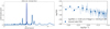 |
Fig. B.1. Periodicities and the power spectral density for the accretion rate in the isotropic Run I. Left: Lomb–Scargle periodogram (power vs. period in years) with the most prominent peak at ∼106 years. Other prominent peaks are at ∼191 and ∼68 years. Right: PSD with the best-fit power-law function with the slope of −0.65 ± 0.17. |
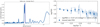 |
Fig. B.2. Periodicities and the power spectral density for the accretion rate in the isotropic Run II. Left: Lomb–Scargle periodogram (power vs. period in years) with the most prominent peak at ∼112 years. Other prominent peaks are at ∼204 and ∼54 years. Right: PSD with the best-fit power-law function with the slope of −0.57 ± 0.12. |
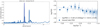 |
Fig. B.3. Periodicities and the power spectral density for the accretion rate in isotropic Run III. Left: Lomb–Scargle periodogram (power vs. period in years) with the most prominent peak at ∼108 years. Other prominent peaks are at ∼190, ∼69, and ∼55 years. Right: PSD with the best-fit power-law function with the slope of −0.49 ± 0.20. |
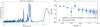 |
Fig. B.4. Periodicities and the power spectral density for the accretion rate in the disk-like Run. Left: Lomb–Scargle periodogram (power vs. period in years) with the most prominent peak at ∼186 years. Other prominent peaks are at ∼217, and ∼100 years. Right: PSD with the best-fit power-law function with the slope of −0.68 ± 0.20. |
Appendix C: Comparison of the IRS 13E X-ray surface-brightness profile with the mock cluster
In this Appendix, we compared the IRS 13E X-ray surface-brightness profile with the one inferred from simulations. In particular, we consider the profiles in two directions: East-West (x) and North-South (y). In addition, we extract the profile of the Chandra point-spread function (PSF). In Fig. C1, we compared the x − y surface-brightness profiles for the observed Chandra image as well as for the simulated one with the Chandra PSF. We see that the observed profile is comparable to the PSF close to the peak, while it is slightly extended toward the tails. The profile constructed from the simulated X-ray image of the compact cluster is consistent with the observed one, except for the wing to the west, where the observed profile is significantly more extended. This can be attributed to the surrounding diffuse X-ray emission and/or individual X-ray sources. This particular bump in the western tail (positive x-direction) was previously attributed to the source E60 (Wang et al. 2020; Zhu et al. 2020).
In terms of the image asymmetry, we compared the observed IRS 13E image with the simulated one using the asymmetry index defined as
 (C.1)
(C.1)
where we subtract the image rotated by 180° from the actual image. The observed image has A = 0.21, while the simulated one has A = 0.13, which is consistent with the simulated image being more symmetric as is also visible in Fig. C1. As we already mentioned, in the observed image, there is a contribution at least from the source E60, which is not a part of the IRS 13E association and as such is not included in the simulated cluster.
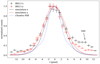 |
Fig. C.1. Comparison of the observed IRS 13E X-ray surface-brightness profiles (black and red points with errorbars in normalized units in two perpendicular directions x and y expressed in pixels) with the corresponding profiles inferred from simulations presented in this study (black and red dashed lines). A dotted blue line depicts the Chandra PSF. The more extended western wing of IRS 13E can be attributed to the E60 source. One pixel is equivalent to ∼0.125 arcsec or ∼5 × 10⁻³ pc at the Galactic center. |
All Tables
Minimum, mean, and maximum distances of all the pairs of six stars (in AU) in the compact cluster and their recurrence timescales corresponding to the most prominent peaks in the Lomb–Scargle periodogram (in years) in the isotropic distribution around the IMBH.
Minimum, mean, and maximum distances of all the pairs of six stars (in AU) in the compact cluster and their recurrence timescales corresponding to the most prominent peaks in the Lomb–Scargle periodogram (in years) in the disk-like distribution around the IMBH.
All Figures
|
Fig. 1. 3D volume rendering of the density of the simulated stellar cluster. Left: Colliding stellar winds 620 years into the Model II spherical simulation. Right: Outbursts of cool clumps 815 years into the Model III spherical simulation, driven by the gas’s higher metal content, which enhances cooling efficiency and amplifies the development of the thin-shell instability. |
| In the text | |
|
Fig. 2. Plane-parallel cuts (y = 0) of fluid quantities for different models. Left and middle columns: Model II without (βw = ∞) and with magnetized winds (βw = 100) 620 years into the simulation. Right column: Model III simulation 815 years into the simulation. Top row: Electron number density ne; Middle row: Accretion rate Ṁ; Bottom row: Temperature. |
| In the text | |
|
Fig. 3. Time and angle-averaged quantities in our simulations as a function of distance from the black hole, r. The different lines denote the different configurations of the simulation. (a) Density in the units of electron number density; (b) Accretion rate Ṁ; (c) Radial velocity of the gas vr; (d) Temperature of the gas. For the density and temperature radial profiles, a line representing ∝r−1 is also plotted for reference, highlighting the approximate power law in both quantities in the inner regions of the simulations. |
| In the text | |
|
Fig. 4. Time and angle-averaged absolute value of the specific angular momentum ⟨|l|⟩ (dashed lines) as well as the absolute value of the average |⟨l⟩| (solid lines) normalized by the Keplerian value, lKep, as a function of distance from the black hole, r. |
| In the text | |
|
Fig. 5. Time and angle-averaged value of plasma β as a function of distance from the black hole, r, for the Model II simulation with magnetized winds using βw = 100. Different lines denote average ⟨β⟩ (solid line), density-weighted average ⟨β⟩ρ (dashed line), and |
| In the text | |
|
Fig. 6. Predicted intrinsic X-ray surface brightness density SX computed from our simulations scaled to Galactic center distance. Left: 650 years into the Model II spherical simulation. Right: 830 years into the Model III spherical simulation. The black hole is visible in the center of the left panel; however, the colliding winds dominate the X-ray emission and, most of the time, make the black hole undetectable (as seen in the right panel). |
| In the text | |
|
Fig. 7. Spectral energy distribution for the accretion flow near the IMBH at the center of the stellar association calculated using a simple ADAF model with a numerical prescription described in Pesce et al. (2021). The input for the model is the time-averaged accretion rate extrapolated to the event horizon of the IMBH (Ṁ = 2.1 × 10⁻¹⁰ M⊙ yr−1) and the associated Eddington ratio (λEdd = 3.168 × 10⁻⁷). For comparison, we also show an SED for Sgr A* calculated with the same model using Ṁ = 2.1 × 10⁻⁸ M⊙ yr−1 and Eddington ratio λEdd = 2.258 × 10⁻⁷. |
| In the text | |
|
Fig. 8. Time evolution of the integrated X-ray luminosity computed from the Model II simulation. Left: X-ray luminosity of a near-horizon ADAF model for the IMBH as well as well as the large-scale emission from the vicinity of the IMBH. Middle: X-ray luminosity of the large-scale flow. Right: IMBH ADAF, IMBH large-scale flow, and total X-ray luminosity combined; we note that the vertical scale is logarithmic. |
| In the text | |
|
Fig. 9. Left: Merged subpixel Chandra image obtained by combining 112 non-grating ACIS-S and ACIS-I observations with a total cleaned exposure time of almost 3.6 Ms. Right: Mock Chandra ACIS-S image obtained using the SOXS simulator based on a Model II spherical simulation snapshot at 50 years. |
| In the text | |
|
Fig. 10. Temporal evolution of the mass inflow rate Ṁ (top row) and mutual distances between the shortest-period star E4 and other stars expressed in au (bottom row) for the isotropic spherical (left column) and disk-like (right column) stellar configurations. The minimum distances for each pair are represented via solid horizontal lines of corresponding color. In both configurations, periodic approaches between the closest star, E4, and all other stars are responsible for the periodic spikes in the inflow rate, with the shortest separations reaching ∼1000 au. |
| In the text | |
|
Fig. 11. Lomb–Scargle periodograms of the X-ray light curves computed from the simulations. Left: LS periodogram of the X-ray light curve produced by the near-horizon flow around the IMBH as calculated from an ADAF model. The highest peak is at ∼210 years, while other prominent peaks are at ∼54 and ∼83 years. The dotted horizontal lines mark inferred confidence levels based on 10 000 bootstrap realizations. Right: LS periodogram of the total X-ray luminosity exhibits the highest peak at ∼104 years. Other prominent peaks are at ∼202, ∼271, ∼55, and ∼74 years. The dotted horizontal lines stand for the confidence levels, as in the left panel. |
| In the text | |
|
Fig. 12. Power spectral densities of the X-ray variability of the compact stellar cluster with an IMBH. Left: PSD of the X-ray light curve produced by the near-horizon flow around the IMBH as calculated from an ADAF model, which has a flat power-law slope of ∼ − 0.53. Right: PSD of the total X-ray light curve, which exhibits a steeper power-law slope of ∼ − 1.41. The points represent mean PSD values within the ten regular logarithmic bins in frequency, while the error bars represent standard deviations in these bins. We fit the power-law functions to these binned PSD values for consistency. In both panels, the extents of the logarithms of PSDs and frequencies are kept the same for consistency and easier comparison. |
| In the text | |
|
Fig. B.1. Periodicities and the power spectral density for the accretion rate in the isotropic Run I. Left: Lomb–Scargle periodogram (power vs. period in years) with the most prominent peak at ∼106 years. Other prominent peaks are at ∼191 and ∼68 years. Right: PSD with the best-fit power-law function with the slope of −0.65 ± 0.17. |
| In the text | |
|
Fig. B.2. Periodicities and the power spectral density for the accretion rate in the isotropic Run II. Left: Lomb–Scargle periodogram (power vs. period in years) with the most prominent peak at ∼112 years. Other prominent peaks are at ∼204 and ∼54 years. Right: PSD with the best-fit power-law function with the slope of −0.57 ± 0.12. |
| In the text | |
|
Fig. B.3. Periodicities and the power spectral density for the accretion rate in isotropic Run III. Left: Lomb–Scargle periodogram (power vs. period in years) with the most prominent peak at ∼108 years. Other prominent peaks are at ∼190, ∼69, and ∼55 years. Right: PSD with the best-fit power-law function with the slope of −0.49 ± 0.20. |
| In the text | |
|
Fig. B.4. Periodicities and the power spectral density for the accretion rate in the disk-like Run. Left: Lomb–Scargle periodogram (power vs. period in years) with the most prominent peak at ∼186 years. Other prominent peaks are at ∼217, and ∼100 years. Right: PSD with the best-fit power-law function with the slope of −0.68 ± 0.20. |
| In the text | |
|
Fig. C.1. Comparison of the observed IRS 13E X-ray surface-brightness profiles (black and red points with errorbars in normalized units in two perpendicular directions x and y expressed in pixels) with the corresponding profiles inferred from simulations presented in this study (black and red dashed lines). A dotted blue line depicts the Chandra PSF. The more extended western wing of IRS 13E can be attributed to the E60 source. One pixel is equivalent to ∼0.125 arcsec or ∼5 × 10⁻³ pc at the Galactic center. |
| In the text | |
Current usage metrics show cumulative count of Article Views (full-text article views including HTML views, PDF and ePub downloads, according to the available data) and Abstracts Views on Vision4Press platform.
Data correspond to usage on the plateform after 2015. The current usage metrics is available 48-96 hours after online publication and is updated daily on week days.
Initial download of the metrics may take a while.