| Issue |
A&A
Volume 702, October 2025
|
|
|---|---|---|
| Article Number | A144 | |
| Number of page(s) | 16 | |
| Section | Stellar structure and evolution | |
| DOI | https://doi.org/10.1051/0004-6361/202555167 | |
| Published online | 20 October 2025 | |
Beyond the Nyquist frequency
Asteroseismic catalog of undersampled Kepler late subgiants and early red giants
1
ENS Paris-Saclay, Université Paris-Saclay, 91190 Gif-sur-Yvette, France
2
Université Paris-Saclay, Université Paris Cité, CEA, CNRS, AIM, F-91191 Gif-sur-Yvette, France
3
Instituto de Astrofísica de Canarias (IAC), E-38205 La Laguna, Tenerife, Spain
4
Institute of Science and Technology Austria (ISTA), Am Campus 1, 3400 Klosterneuburg, city Austria
5
Universidad de La Laguna (ULL), Departamento de Astrofísica, E-38206 La Laguna, Tenerife, Spain
6
Department of Astronomy, The Ohio State University, Columbus OH 43210, USA
7
Institute of Space Sciences (ICE, CSIC), Carrer de Can Magrans S/N, E-08193 Cerdanyola del Vallès, Spain
8
Institut d’Estudis Espacials de Catalunya (IEEC), Carrer Esteve Terradas, 1, Edifici RDIT, Campus PMT-UPC, E-08860 Castelldefels, Spain
9
Department of Physics and Astronomy, California State University, Long Beach, Long Beach CA 90840, USA
10
Department of Astronomy, University of Florida, Gainesville FL 32611, USA
11
Department of Physics, The Ohio State University, Columbus OH 43210, USA
⋆ Corresponding author.
Received:
15
April
2025
Accepted:
24
July
2025
Abstract
Subgiants and early red giants are crucial for studying the first dredge-up, a key evolutionary phase in which the convective envelope deepens, mixing previously interior-processed material and bringing it to the surface. Yet, very few have been seismically characterized with Kepler because their oscillation frequencies are close to the 30 minute sampling frequency of the mission. We developed a new method as part of the new PyA2Z code of identifying super-Nyquist oscillators and inferring their global seismic parameters, νmax and large separation, Δν.
Applying PyA2Z to 2065 Kepler targets, we seismically characterize 285 super-Nyquist and 168 close-to-Nyquist stars with masses from 0.8 to 1.6 M⊙. In combination with APOGEE spectroscopy, Gaia spectrophotometry, and stellar models, we derive stellar ages for the sample. There is good agreement between the predicted and actual positions of stars on the HR diagram (luminosity vs. effective temperature) as a function of mass and composition. While the timing of dredge-up is consistent with predictions, the magnitude and mass dependence show discrepancies with models, possibly due to uncertainties in model physics or calibration issues in observed abundance scales.
Key words: asteroseismology / methods: data analysis / stars: evolution / stars: interiors / stars: oscillations
© The Authors 2025
 Open Access article, published by EDP Sciences, under the terms of the Creative Commons Attribution License (https://creativecommons.org/licenses/by/4.0), which permits unrestricted use, distribution, and reproduction in any medium, provided the original work is properly cited.
This article is published in open access under the Subscribe to Open model. This email address is being protected from spambots. You need JavaScript enabled to view it. to support open access publication.
1. Introduction
Turbulence in the outer layers of cool stars excites oscillations (Goldreich & Keeley 1977; Kumar et al. 1988). Asteroseismology, the characterization of the properties of stars through the analysis of oscillation modes (Christensen-Dalsgaard 1984), has proven to be a valuable tool in studying solar-like pulsating stars. The characteristic oscillation frequencies are proportional to the mean density; they range from 5 minutes for solar analogs, hours to days for low- and mid- luminous red giant stars (RGs), on the order of 5 hours for core He-burning (RC) stars, to months or years for the most luminous ones on the red giant branch (RGB) (Mosser et al. 2019).
With the advent of large time-domain surveys from space missions, these oscillations became detectable for large numbers of stars. However, previous studies have generally been dominated by evolved RGs, which have higher amplitudes and lower oscillation frequencies. These frequencies can generally be detected in the baseline observing mode of the instruments performing the surveys, such as long cadence (LC) in the Kepler mission (Borucki et al. 2010) and full-frame image data from the Transit Exoplanet Survey Satellite (TESS, Ricker et al. 2014), and therefore require less specific and deliberate targeting. Several hundred thousand RGs on the RGB and red clump (RC) have been analyzed using asteroseismology (e.g. De Ridder et al. 2009; Huber et al. 2010; Mosser et al. 2010; Stello et al. 2015, 2017; Anders et al. 2016; Yu et al. 2018; Zinn et al. 2020, 2022; Hon et al. 2021; Li et al. 2022).
Seismic observers have also been particularly interested in the solar-like oscillations of main-sequence dwarf stars (García & Ballot 2019). They require special observation modes with shorter cadences. By contrast, only around 1000 main sequence solar-like oscillators have been seismically characterized (e.g. Benomar et al. 2009; Ballot et al. 2011; Davies et al. 2015, 2016; Serenelli et al. 2017; Silva Aguirre et al. 2017; Ong et al. 2021; Huber et al. 2022; Mathur et al. 2022; González-Cuesta et al. 2023; Hatt et al. 2023; Lund et al. 2024). The domain between the main sequence and the giant branch, referred to as the subgiant branch, is astrophysically interesting. However, stars in this domain have neither been targeted as planet-host candidates nor have they exhibited detectable oscillation modes in LC data. As a consequence, this subgiant transition zone is much more poorly understood, and it is clear that important physical processes occur in cool subgiants. At this evolutionary stage, nuclear burning ceases in the core and fusion is ignited in a shell surrounding it. The core contracts and the envelope expands in these stars, affecting their radial rotation profile, which exhibits strong internal differential rotation (e.g. Beck et al. 2012; Deheuvels et al. 2012, 2014). This core contraction also influences their magnetic fields and activity (e.g. García et al. 2014b; Godoy-Rivera et al. 2021; Metcalfe et al. 2024). The hydrogen-exhausted cores also become dense, and at low mass degeneracy pressure sets in. At the same time, the fully mixed surface convection zone deepens. This causes the products of core nuclear processing appear at the surface as stars develop deep surface convective envelopes (Roberts et al. 2024). This first dredge-up (FDU; Iben 1965; Salaris et al. 2015) has been used as a mass and age diagnostic for stellar populations (Martig et al. 2016; Ness et al. 2016) and is a key prediction of stellar theory. All of these processes are very sensitive to the details of the physics of the stellar interior and impact the future evolution of the star, including the expected nucleosynthesis (Karakas & Lattanzio 2014) and the resulting remnant (Hermes et al. 2017). Unfortunately, only a select number of subgiant and lower giant stars have been the subject of the asteroseismic observations that are necessary for their masses to be constrained and their interior structures to be probed.
This relative lack of subgiant data is largely due to the observing strategies employed by space missions. The first generation of space time-domain missions, such as Convection Rotation and planetary Transit (CoRoT, Baglin et al. 2006), Kepler, and K2 (Howell et al. 2014), use relatively long observing baseline cadences optimized for transits of Earth-likeplanets around Sun-like stars. For example, Kepler offers two acquisition modes: short cadence (SC, sampling period Tsamp = 58.85 s and Nyquist frequency (defined as νNyq = 1/2Tsamp) νNyq ≃ 8496 μHz, Gilliland et al. 2010) and long cadence (LC, sampling period Tsamp = 29.4 min and νNyq ≃ 283 μHz, Jenkins et al. 2010). While most of the stars were observed in LC mode (197 096 targets for Kepler, Mathur et al. 2017; Godoy-Rivera et al. 2025), at any time only 512 slots were allocated for SC observations. Although subgiant stars could be observed in this SC mode, the asteroseismic community privileged the study of main-sequence stars and early subgiants. As a result, only a few late subgiants and early RGBs were targeted.
Murphy et al. (2013) showed that it was possible to recover the parameters of δ Scuti oscillating above the Nyquist frequency and Chaplin et al. (2014) showed that cool, evolved subgiants and stars lying at the base of the RGB, whose oscillation frequencies are well above the νNyq, could be studied with the LC Kepler dataset by using the aliased frequencies below νNyq. They called it “Super-Nyquist asteroseismology”. This methodology was further exploited by Mathur et al. (2016) and Yu et al. (2016), providing detections of oscillations in 47 stars in the super-Nyquist regime, up to a maximum power frequency of νmax = 387 μHz, using LC Kepler data.
In this paper, we develop a new methodology to study the pattern of modes around νNyq and disentangle whether those modes are sub-Nyquist, super-Nyquist, or if they are centered around Nyquist (hereafter close-to-Nyquist). This results in a large sample of late subgiants and early RGs that allow us to study the FDU. Our work complements the recent APOKASC-3 paper (hereafter APOKASC-3, Pinsonneault et al. 2025), which provided asteroseismic data for stars with Kepler light curves and Apache Point Observatory Galactic Evolution Experiment (APOGEE, Majewski et al. 2017) spectra. In that study, it was found that different methods diverged for νmax > 220 μHz, so no stellar parameters were inferred for such stars there. The upcoming García et al. catalog (in prep.) provides similar data for stars with νmax < 220 μHz, which do not have APOGEE spectra. In this work, our analysis includes all Kepler stars with νmax > 200 μHz, and complements these other two papers. In Section 2, the observations used in this paper as well as the sample selection of stars are described. The principles behind the classification of stars as sub-Nyquist, close-to-Nyquist, or super-Nyquist are described in Section 3 and the results are presented and discussed. In Section 4, we compute the stellar parameters (masses, radii, and ages) from stellar models and we discuss how the sample probes the FDU phase in Section 5. The conclusions are given in Section 6.
2. Sample selection and data preparation
One of the objectives of this paper is to compile the most complete catalog of pulsating late subgiants and early RGs observed by Kepler in LC, crucial for advancing the asteroseismology of solar-like stars with νmax > 200 μHz and studying the dredge-up. A paramount consideration in this endeavor is the avoidance of any selection bias, which holds immense significance for Galactic archaeology and stellar population studies.
Briefly, the initial set of stars in APOKASC-3 and García et al. (in prep.) is a compilation of 30 336 Kepler targets selected to be potential subgiants and RGs. The starting point is the catalog of 16 094 confirmed RGs from Yu et al. (2018), which included previous detections (Hekker et al. 2011; Huber et al. 2011; Stello et al. 2013; Huber et al. 2014; Mathur et al. 2016; Yu et al. 2016). Then, subgiants and RGs not included in the previous set were added from the Kepler DR25 catalog (Mathur et al. 2017), the Kepler-Gaia DR2 catalog (Berger et al. 2018), the DR16 and DR17 of the APOGEE spectroscopic survey (Ahumada et al. 2020; Abdurro’uf et al. 2022), and other seismic RGs found during the visual inspections done for the surface rotation-period catalogs by Santos et al. (2019) and Santos et al. (2021).
From these samples, our stars were selected following a multistep process. We first selected stars from the APOKASC-3 catalog (i.e., with APOGEE spectra, see Section 4.1) with a seismic νmax > 200 μHz. Then, we added stars from García et al. (in prep.), not included in APOKASC-3, and with a seismic νmax > 200 μHz. This differs from the νmax = 220 μHz cutoff in the APOKASC-3 sample, as our goal was to ensure the most complete initial sample considering larger uncertainties on the García et al. (in prep.) values. This led to an initial sample of 1959 stars with seismic inferences. This sample will be referred to as the “main sample” in the rest of the paper. Finally, we included 106 stars from the APOKASC-3 catalog without seismic detections (i.e., not already included in our sample) but with a predicted frequency of maximum power from spectroscopy, νmax, spec > 180 μHz (as already done in e.g. Beck et al. 2018). This sample will henceforth be referred to as the spectroscopic sample.
This threshold of 180 μHz is lower than the 200 μHz one used for the main sample to better account for the larger uncertainties on the spectroscopic parameters (σlog g = 0.065). This predicted νmax, spec was computed from seismic scaling relations (Brown 1991; Kjeldsen & Bedding 1995) as follows:
 (1)
(1)
where gspec and Teff are, respectively, the APOGEE spectroscopic surface gravity and effective temperature of the star. Those parameters and the way we obtained them will be further developed in Section 4.1.
The Kepler seismic analyses were done using KEPSEISMIC1 light curves filtered at 20 days obtained from the Mikulski Archive for Space Telescopes (MAST) archive. They were corrected with the Kepler Asteroseimic data analysis and calibration Software (KADACS, García et al. 2011), to remove outliers, correct any jumps and drifts, and stitch together the Kepler quarters. All the gaps were interpolated using in-painting techniques based on a multi-scale discrete cosine transform (García et al. 2014a; Pires et al. 2015).
3. Classification of close-to- and super-Nyquist stars
When the oscillations of a star are undersampled, its power spectrum undergoes a symmetry operation and its mode frequencies are reflected about the νNyq frequency. This paper considers two cases of undersampling: stars with modes very close to the Nyquist frequency (hereafter close-to-Nyquist stars) and stars with modes above the Nyquist frequency (super-Nyquist stars). For the close-to-Nyquist stars, when the modes above νNyq are reflected, they overlap with the ones below νNyq (see Fig. 1, panel (a)). For the super-Nyquist stars, when the modes are reflected below νNyq (see Fig. 1, panel (b)), they remain isolated under the Nyquist frequency.
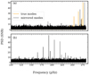 |
Fig. 1. Power spectral density (PSD) of two simulated stars in units of the signal-to-noise ratio (SNR) as a function of frequency. Panel (a): Star with modes close to νNyq at the right edge of the frequency range. The true modes are in orange and the mirrored modes in black. Panel (b): Star with super-Nyquist modes where only the folded modes are observed between 0 μHz and νNyq. |
Symmetry is isometric, meaning that folding preserves the distances between modes. In particular, for a star for which the frequencies of the modes follow the asymptotic distribution (Tassoul 1980), the frequencies of the modes, νn, l, roughly follow the pattern
 (2)
(2)
where n is the order of the mode, l is its degree, and ε is the phase term. This equation means that the modes of the odd angular degree are found halfway between the modes of even degree. The dipole modes will be in between the radial modes, creating a periodicity in  in the power spectrum density (PSD). This periodicity is preserved by symmetry so long as the spectrum is not folded onto itself. Moreover, when getting closer to νmax, the PSD of the PSD will show an increase in power at
  . These phenomena allow one to search for the seismic parameters to measure both νmax and Δν.
By isometry of the symmetry operation, the Δν measured on a folded spectrum will be correct. As for νmax, if the real modes were indeed below νNyq then the measured νmax (νmax, measured) would be the correct one. However, if the real modes were above the Nyquist frequency, we carried the measurement of νmax on a symmetrized oscillation spectrum. Hence, in this case, the real νmax should by symmetry be located at 2νNyq − νmax, measured.
Without prior information to find out whether a star has a folded spectrum or not, we used a simple test: the pair of the set {(Δν,νmax,measured),(Δν, 2νNyq − νmax,measured)} that best matched the seismic scaling relation Δν ∝ νmax0.77 (Stello et al. 2009) was assumed to be the correct pair of parameters.
3.1. Measuring global seismic parameters in the sub- and super-Nyquist regimes
Before performing the seismic analysis, the components of the power spectrum arising from sources other than the oscillations, mostly convection and instrumental effects, should be removed. Generally, this is done by fitting the convective background with different components, including Harvey-likemodels (Harvey et al. 1985), the p-mode envelope, and the photon noise (e.g. Mathur et al. 2011; Corsaro & De Ridder 2014; Kallinger et al. 2014). To flatten down the PSD, it is enough to use a median filter to characterize the background level at each frequency, as is shown in Fig. 2. The resulting background estimate is then used to normalize the PSD by division.
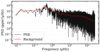 |
Fig. 2. PSD of the star KIC 8179973 and estimate of its background with a median filter. |
3.1.1. Measuring νmax,sub of the sub-Nyquist PSD
Without prior information on the star, it is not possible to discriminate between a sub- or super-Nyquist star. We applied the PyA2Z pipeline (Liagre et al., in prep.), which is the new Python version of the A2Z pipeline (Mathur et al. 2010), to estimate the global seismic parameters of solar-like oscillations.
We began by determining the apparent νmax below νNyq (hereafter νmax,sub) without any prior guess. We note that in the case of a super Nyquist star, where the modes are mirrored across the Nyquist frequency, that this will not correspond to the true νmax value. For instance in Fig. 1(b) the observed modes are those of a mirrored super Nyquist star, and therefore the directly measured νmax,sub (201 μHz) will not correspond to the true νmax (365 μHz).
To measure νmax,sub, PyA2Z relies on the periodicity of the acoustic modes in the PSD. As is explained in Sect. 3 the PSD of the PSD (hereafter PS2) in a region containing modes should show a power excess around  . The power excess should be at its maximum in the region around νmax,sub, assuming that the mode amplitudes follow a Gaussian envelope.
Therefore, the pipeline measured νmax,sub as follows (the process is illustrated in Fig. 3):
-
A segment of the PSD was selected on a box centered on νcenter and of width
 . We used a typical value of Γ = 2. The parameters β and α are given by the scaling relation
  , with α ≈ 0.77 following Stello et al. (2009) and
  being normalized to the solar value. The key idea behind this is that if νcenter = νmax then we select ≈3 × Γ peaks, which is enough to compute the PS2 and detect the
  periodicity without having to deal with unwanted noise. If the box is too big, the χ2 noise of the PSD will pollute the PS2 and that can result in a reduced sensibility or a nondetection of the modes, whereas if the box is too small, not enough modes will be present to ensure the periodicity detection by the PS2 method. Local deviations from the asymptotic pattern (e.g. glitches, Mazumdar et al. 2012, 2014) are not expected to have a significant impact on the measurement of νmax as these would effectively be averaged out by our global analysis.
 -
The algorithm computed the PS2 of that segment and filtered it around the expected positions of
 and
and  (given by the scaling relation
  ) assuming νcenter = νmax,sub (see inset of Fig. 3(a)).
 -
The filtered PS2 was then averaged and that average was stored in an array, A.
-
The box was slid up to higher frequencies by a fraction, s, of Δν and the algorithm went back to step 1 until it reached the Nyquist frequency.
-
Once the box was at the Nyquist frequency, a Gaussian function was fit to A as a function of νcenter. The mean of the fit Gaussian function was then our measure of νmax. This measure also provided the standard deviation of the fit Gaussian function, σnm, which was used as a proxy for the width of the amplitude envelope of the mode. Several tests with Markov chain Monte Carlo (MCMC) methods have shown that very little uncertainty comes from the fitting process itself (typically less than 1 μHz on the range of frequencies observed). Pinsonneault et al. (2018) showed that the uncertainty is largely dominated by the dispersion of the values obtained by different seismic pipelines. For that reason, we ignored the errors coming from the fitting process and decided to conservatively assign an error bar of
 to our measurement for νmax. This error bar comes from the fact that, νmax being an observational parameter, it is limited in precision by the density of modes in the envelope and these are asymptotically distinct by
  .
.
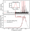 |
Fig. 3. (a) PSD of the Kepler star KIC 8179973 on which a sliding box (shaded pink area) was used to compute the PS2 (inset) with Γ = 2 and filtered as explained in Section 3.1.1. (b) The red line is the averaged filtered PS2 normalized to its maximum value as a function of the center of the sliding windows. The dashed black line is the Gaussian fit. |
3.1.2. Measuring Δν
Once νmax was measured, the PSD was filtered by a zero padded hanning window around it. The filter, F, is defined as follows:
 (3)
(3)
where m ≈ 4.3 has been found to give precise Δν without too much sensitivity to the noise in the PSD. The PS2 of that filtered PSD was then computed and the region where the peaks associated with  and
and  were expected was once again selected. Assuming that the modes frequencies follow an asymptotic pattern with typical amplitudes and widths, the properties of the Fourier transform lead to a higher peak at
  than at
  in the PS2. Thus, a Gaussian function was fit to the highest peak providing a measure for
  . The standard deviation of the fit Gaussian function was taken as the uncertainty over the
  measure and that uncertainty was propagated on Δν following the usual formula:
  , where u(Δν) and
  are the uncertainties on Δν and
  , respectively.
3.2. Undersampled super-Nyquist stars
When a star is undersampled, i.e., some mode frequencies are super-Nyquist, its oscillation spectrum is folded around the Nyquist frequency. This yields a mirrored spectrum that in some cases overlaps with sub-Nyquist non mirrored modes. As is stated in Section 3, assuming that the true νmax is sufficiently far beyond the Nyquist frequency, the modes observed in the mirrored PSD will not overlap with the modes existing below νNyq because their height will be negligible compared to the mirrored ones (as in Fig. 1(b)). We have realized that when the star is undersampled and  , the overlapping effect of the modes is negligible (where FWHM stands for full width at half maximum and is the width of the Gaussian envelope of the modes at half its maximum). Using the scaling relation FWHM = 0.25νmax (Lund et al. 2017), this condition is equivalent to having νmax > 323 μHz. We then classified the stars with νmax > 320 μHz as super-Nyquist, those with νmax between 250 μHz and 320 μHz as close-to-Nyquist stars, and those under 250 μHz as sub-Nyquist stars.
As was previously explained in Section 3, we tested which pair of the set {(Δν, νmax, measured),(Δν, 2νNyq − νmax, measured)} best follows the scaling relation Δν ∝ νmax0.77. That was used to identify the true νmax, whether it was the one mirrored around νNyq or the directly measured one νmax,sub. This determined the final classification as sub-Nyquist, close-to-Nyquist, or super-Nyquist. The whole algorithm is visually described by a flowchart in Appendix A.
To quantify the apodization effects (see Appendix C) on the super-Nyquist measurement of νmax, we extracted the seismic properties of three real Kepler subgiants observed in SC that we used to simulate LC observations. Then, we followed the procedure described below:
-
For each of the three stars, we fit their modes in the PSD of the SC dataset using the Python library apollinaire (Breton et al. 2022, 2023) and the Python tool iechelle2. Since the SC timeseries have a Nyquist frequency of 8496 μHz, the apodization effect in the PSD of a star with νmax between 300 and 400 μHz is negligible (indeed, the change in the apodization function on that frequency range is very small,
 ).
). -
With the fit mode parameters, we simulated a light curve with 20 × 1440 days3 using a sampling period of 1 min and the same noise level as the original Kepler observations. For each star we performed Monte Carlo simulations with 500 different noise realizations.
-
From that SC light curve, we extracted a 4-year-long rebinned one at the Kepler LC rate of 29.4 minutes.
-
Finally, we ran PyA2Z on both the SC and the rebinned LC light curves and we compared the results.
The MC simulation shows a systematic effect of underestimating νmax in the super-Nyquist regime, which is consistent with what we expect from theory. As the apodization function, η2, is a decreasing function on the range [0, 566] μHz, we expect the Gaussian envelope of the modes to be skewed toward the lower frequencies below its mean value. This result also confirms that the error bar of  is appropriate because, for more than 99.93% of the realizations, the extracted νmax of both cadences agree within their uncertainties.
3.3. Handling close-to-Nyquist stars
For close-to-Nyquist stars, the measurement of νmax is more complicated. The envelope of the modes consists of two overlapping Gaussian envelopes: one corresponding to the sub-Nyquist modes and the other to the mirrored super-Nyquistmodes.
In this context, it is crucial to distinguish the real modes from the mirrored ones, to mask them and measure νmax. To do so, the method we used was based on a straightening of the ℓ = 0 ridge of the echelle diagram. Given that the operation of symmetry does not affect the periodicity in Δν of the spectrum, a first measure of Δν was inferred from the PSD by the method described in Sect. 3.1.2.
To construct the echelle diagram, the PSD was mirrored above νNyq and concatenated with itself, as is shown in Fig. 4(a), using only ℓ = 0 and 2 modes. This ensured that, once the echelle diagram was constructed, both ridges due to the real modes and those due to the mirrored modes were present and aligned as shown in Fig. 4(b).
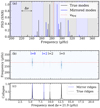 |
Fig. 4. (a) Synthesized PSD of the ℓ = 0, 2 modes of a star with νmax = 275 μHz. The black modes are the true modes, whereas the blue modes are those observed because of the undersampling: they are the black modes mirrored around νNyq. Each box of width Δν matches to one line of the echelle diagram shown in panel (b) along with its collapse in (c). In (b), the ridges due to the true modes are annotated in black, whereas those annotated in blue are due to the shadow modes. In (c) the peaks due to the mirrored modes are marked with a vertical dashed blue line and the peaks due to the true modes are marked with a vertical dotted black line. |
The straightening algorithm consists of varying the assumed Δν around the initial guess to maximize the amplitude of the ℓ = 0 peaks (due to the shadow and true ridges) in the collapse of the echelle diagram. Once that maximization was done, the algorithm proceeds to a peak detection and finds the candidates for the ℓ = 0 and ℓ = 2 ridges. The correct pair of ridges is found by searching for the set of peaks in the collapsed echelle diagram following the scaling relation δν0, 2 ≈ 0.123Δν in Corsaro et al. (2012).
Once that detection was done, the true ℓ = 0 modes were isolated in the PSD, the apodization was corrected by dividing the amplitudes of the modes by η2 (see Appendix C), and νmax was measured again. The uncertainty on νmax is once again given by  . However, since the method straightens the ridges of the echelle diagram to get a measure of Δν, the optimization process makes it challenging to compute a reliable value of the uncertainty on Δν. To be conservative, we set a 10% relative uncertainty on Δν, corresponding approximately to the maximum uncertainty found in this work for the sub- and super-Nyquist samples.
3.4. Global seismic parameters
Among the 2065 stars of our sample defined in Sect. 2, our pipeline PyA2Z presented in Sect. 3, along with a visual inspection, allowed us to reclassify 285 stars as super-Nyquist (see Table 1 and Table 2). Furthermore, it measured the global seismic parameters of 168 close-to-Nyquist stars (see Table 1 and Table 3).
Number of stars analyzed in each category.
Global seismic parameters from the confirmed 285 super-Nyquist stars.
Global seismic parameters from the confirmed 168 close-to-Nyquist stars.
Among the super- and sub-Nyquist stars, 309 lack global seismic parameters (taking into account the main and the spectroscopic samples). These can be explained by different factors such as the absence of a detectable signal above 150 μHz in the PSD (labeled as “No signal” in Table 1), a failure of the pipeline to determine Δν (labeled as ’No Δν’ in Table 1), spikes (usually stemming from a companion object or instrumental effects) that could not be properly removed (labeled as “Spikes” in Table 1), contamination in the light curve (labeled as “Contamination” in Table 1), and the pipeline’s inability to converge during the fitting process (labeled as “Pipeline failure” in Table 1). Thirty-six stars in the sample have a detection of νmax and Δν for which we are unsure of the correctness of the result (because the visual inspection of the echelle diagrams could not confirm the detection); they are labeled as “Dubious” in Table 1). Hence, they were excluded from the final table.
Of the 591 close-to-Nyquist stars, our pipeline successfully provided measurements of Δν and νmax for 28% of them. Most of the initial pipeline’s misdetections were due to a measurement of the second harmonic of the Δν periodicity in the PS2 (peak corresponding to  ) instead of the first (peak at
  ). This problem, which was observed several times upon visual examination of the measurements, was most prominent when the power in the ℓ = 1 was not as high as expected (for instance in the PSDs of depressed dipole mode stars, e.g. García et al. 2014b). This phenomenon arises when the amplitudes of the ℓ = 1 modes are reduced, the dominant periodicity of the PSD asymptotically becomes Δν, and we no longer observe the significantly greater peaks at
  harmonics as is expected in the case of a
  dominant periodicity of the PSD. This observation led to the implementation of a test for flagging depressed dipole modes stars in our dataset: if the ratio of the heights of the peaks of two consecutive peaks at
  and
and  , k ∈ ℕ of the PS2 was close to 1, the star was flagged and a visual inspection was made to confirm whether the dipole modes are indeed depressed or not.
Among the 47 stars with νmax above the Nyquist frequency in Yu et al. (2016) we confirmed the global seismic parameters of 46 of them. However, for KIC 4759008, our analysis –including a visual inspection– cannot confirm the published value.
Our methodology increased the sample of stars with νmax > 283 μHz (which includes super-Nyquists stars as well as some close-to-Nyquist stars) by a factor of 7. The stars we have detected along with the scaling relation we used are plotted in Appendix B.
Since TESS observations have shorter cadences compared to Kepler after cycle 34 (10 and 3 minutes, respectively, for cycles 3 and 4 and from cycle 5 onward), our Kepler stars are not super-Nyquist in these TESS data and could be analyzed using traditional asteroseismic methods. Thus, we have studied all our stars that have been observed in the two TESS extended missions and for which the Quick Look Pipeline (QLP, Huang et al. 2020a,b; Kunimoto et al. 2022) data are available (see Appendix D). Unfortunately, most of the Kepler stars are too faint to have measurable oscillations in TESS. We were able to perform the seismic analysis in only nine stars (see Fig. D.1). For all of them, we measured a νmax from TESS that is consistent with our claimed νmax value from Kepler (see Table D.1). Given that this sample includes two stars that we identified as super-Nyquist, this gives us additional confidence that our methods are correctly obtaining the true νmax from the Kepler data.
4. Fundamental stellar parameters
Asteroseismology, Gaia data, and spectroscopic surveys make for a powerful combination. Indeed, precise and accurate Gaia luminosities, combined with Teff, provide an independent measure of radius that can be used to test asteroseismic scaling relations. The asteroseismic scaling relations require direct knowledge of Teff. Mapping Δν to the mean density and age requires knowledge of the heavy element abundance mixture. We therefore begin by summarizing the spectroscopic data that we have used, and follow with our method of inferring mass, radius, and age.
4.1. Atmospheric parameters
High-resolution spectroscopy is uniquely capable of measuring stellar abundances. We adopted [Fe/H] and [α/Fe] to characterize the abundance pattern relative to a reference solar mixture (see APOKASC-3 for a discussion). Our stellar models and inferences use the Grevesse & Sauval (1998) heavy element mixture for the Sun, which is in good agreement with helioseismic data (Basinger et al. 2024). Spectroscopic Teff data can be tied to an absolute scale, and these Teff estimates are less susceptible to uncertainties arising from interstellar extinction than Teff inferred from characterizing the spectral energy distribution. Spectroscopic data are therefore highly desirable for precise and accurate stellar characterization (Casagrande et al. 2010; González Hernández & Bonifacio 2009).
APOGEE is part of the Sloan Digital Sky Survey (SDSS; York et al. 2000), which has now gone through five major surveys and 17 data releases. Data in the Kepler fields were obtained during SDSS-III (Eisenstein et al. 2011) and SDSS-IV (Blanton et al. 2017). APOGEE is a multi-fiber survey that uses a high-resolution (R ∼ 22 000) infrared spectrograph (Wilson et al. 2019) mounted on the SDSS telescope (Gunn et al. 2006). APOGEE targeting, described in Zasowski et al. (2013, 2017), Beaton et al. (2021), focused on the Kepler fields largely because of the overlap with asteroseismic targets. Stellar parameters were inferred using amultidimensional chi-squared analysis technique, the ASPCAP pipeline (García Pérez et al. 2016), and were tied to a fundamental scale in a post-processing step. The Teff scale is the González Hernández & Bonifacio (2009) calibration of the infrared flux method. We used the latest public data, Data Release 17 (hereafter DR17, Abdurro’uf et al. 2022). Median uncertainties in Teff, [Fe/H], and [α/Fe], as is discussed in Pinsonneault et al. (2025), are 42K, 0.05 dex, and 0.05 dex, respectively. These data are also our sole source of [C/Fe] and [N/Fe], important for testing the FDU of CNO cycle processed material in RGs (see below).
We did not have spectra for all of our targets, however, and as a result we needed to expand our methodology to include information from other sources. Atmospheric parameters from APOGEE DR17 were used in priority when available, and we completed the sample with the Gaia XP spectra (R ∼ 100; Carrasco et al. 2021). These data have been used to infer abundances and Teff for 175 million stars, using APOGEE DR17 as the training set for the XGboost algorithm (Chen & Guestrin 2016), leading to the catalog by Andrae et al. (2023). For the 1321 stars that we classified as sub-, close-to-, and super-Nyquist (see Section 3.4), 640 stars have APOGEE parameters and 1249 stars have XGBoost values with an overlap for 611 stars. With this, we are left with 43 stars that lack spectroscopic and spectrophotometric parameters.
4.2. Computing the stellar fundamental parameters
The computation of stellar masses, radii, and ages was done with BeSPP (Serenelli et al. 2013, 2017) and followed the methodology used for the APOKASC-3 catalog of evolved stars (Pinsonneault et al. 2025). We used a grid of stellar models computed with GARSTEC (Weiss & Schlattl 2008) that spans the mass range between 0.6 and 5 M⊙, and −2.5 and +0.6 for [Fe/H]. It is the same grid used in Pinsonneault et al. (2025) and a detailed description of the physical inputs of the stellar models can be found in that work. Spectroscopic stellar parameters were adopted from APOKASC-3 where available, and otherwise from XGBoost (see Sect. 4.1).
Seismic quantities for each model of the grid were computed as follows. νmax was computed from the scaling relation
 (4)
(4)
where g and Teff are the surface gravity and effective temperature of the models. Δν was computed as the slope of a linear fit to the frequencies of radial modes with frequencies lower than the acoustic cutoff frequency. For the fit, frequencies were weighted assuming a Gaussian envelope centered in νmax with a FHWM given by 0.66νmax0.88 (Mosser et al. 2012). The ratio
 (5)
(5)
measures the deviation of stellar models away from a strict scaling relation between Δν and the square root of the mean stellar density. From the relations above, mass and radius can be formally obtained from
 (6)
(6)
and
 (7)
(7)
We have chosen solar reference values to be consistent with APOKASC-3 (νmax, BeSPP, ⊙ = 3076 μHz and Δν⊙ = 135.146 μHz) and we have used a constant fνmax = 0.996: the correction to the solar νmax computed in APOKASC-3 for stars with νmax > 50 μHz (Pinsonneault et al. 2025).
The first step in the calculation of stellar fundamental parameters is to use Δν, νmax and Teff in Eqs. (4) and (6) to compute g and M, assuming fΔν = 1, i.e., perfect scaling relations. We used M, g, and [Fe/H]corr5 as input quantities in BeSPP to produce a posterior distribution of fΔν and then an updated stellar mass using Eq. (6). The process was continued iteratively until convergence for fΔν was obtained when changes in fΔν were smaller than one part in 105, typically requiring three to five iterations. The final seismic stellar mass and radius, and their uncertainties, were then obtained using Eqs. (6) and (7) one last time. We note that, since the XGBoost dataset does not include measurements of [α/Fe], we adopted [α/Fe] = 0 when using this data. To account for the additional uncertainty introduced by this assumption, we inflated the reported uncertainties from 0.1 dex to 0.15 dex in metallicity and from 50 K to 70 K in effectivetemperature.
To determine the age, we ran BeSPP again, using g, [Fe/H]corr, and the seismic mass as inputs. However, the age dependence on stellar mass departs from a local linear behavior when mass uncertainties are not small. In order to provide age central values and uncertainties that are consistent with those of the seismic masses, we proceeded as follows. BeSPP was run three times using as an input in each of the runs, respectively: the central seismic mass, the central mass increased by its uncertainty, and the central mass decreased by its uncertainty. For each of the three runs, a small formal mass uncertainty of 0.01 M⊙ was used; this does not reflect the true uncertainty, which was instead accounted for by considering the spread across the three runs. The first run was used to determine the central value of the age of the star and the standard deviation was assumed to represent uncertainties linked to g and [Fe/H]corr uncertainties. The other two runs were used to compute the −1σ and +1σ age uncertainties, respectively, after quadratically adding the standard deviations from the central run.
4.3. Comparison with Gaia
In order to vet the asteroseismic results, we compared them to alternate radius and mass scales using Gaia radii. We used Gaia DR3 parallaxes (Gaia Collaboration & Vallenari 2023; Lindegren et al. 2021b) as the basis for a luminosity scale, corrected according to Lindegren et al. (2021a) and with non-single stars removed as well as spurious parallax solutions (Rybizki et al. 2022). These parallaxes, when combined with extinctions, 2MASS K-band photometry, and bolometric corrections, as well as spectroscopic temperatures, will yield a radius; this approach has been detailed in Zinn et al. (2017). As in Sect. 4.2, spectroscopic stellar parameters were adopted from APOKASC-3 where available, and otherwise from XGBoost. The K-band bolometric correction was interpolated from MIST (Choi et al. 2016; Dotter 2016; Paxton et al. 2011, 2013, 2015) bolometric correction tables in metallicity, gravity, and temperature. The tables were constructed using the C3K grid of 1D atmosphere models (C. Conroy et al., in preparation; based on ATLAS12/SYNTHE; Kurucz 1970; Kurucz et al. 1993). Salaris-corrected metallicities were adopted (Salaris et al. 1993) when [α/Fe] was available from APOKASC-3 and otherwise we assumed [α/Fe] = 0 with an uncertainty of 0.3dex. Finally, K-band magnitudes were required to have an “A” quality rating from 2MASS. We used asteroseismic surface gravities for the bolometric calculation, and therefore we only included stars with measured νmax. Extinctions were calculated using a three-dimensional dust map based on Marshall et al. (2006), Green et al. (2019) and Drimmel et al. (2003), as implemented in mwdust (Bovy et al. 2016). Δν values were corrected with the fΔν scale from asfgrid (Sharma et al. 2016; Stello & Sharma 2022). For this purpose, evolutionary states were taken to be RGB unless they were categorized as “RC” in APOKASC-3.
Figure 5 shows excellent agreement between asteroseismic and Gaia radii – to within 0.9% on average. The sample presented here lies between the two radius regimes in which (Zinn et al. 2019) quantified the asteroseismic and Gaia radius scale agreement. In that work, stars with R < 3.5R⊙ were found to have a ratio of Rastero/RGaia = 0.979 ± 0.005 and stars with 10R⊙ < R < 30R⊙ were found to have a ratio of Rastero/RGaia = 1.019 ± 0.006. In our intermediate radius regime, the agreement lies between these values, suggesting a smooth transition in systematics – related to either scaling relations or perhaps temperature scales – between the dwarfs and giants (see also Fig. 3 of Zinn et al. 2019.)
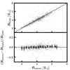 |
Fig. 5. One-to-one comparison of Gaia and asteroseimsic radius scales (top) and the fractional differences (bottom; with binned medians and uncertainties on the median). The two show excellent agreement (to within 0.9% on average), which demonstrates the accuracy of the asteroseismic analysis here and of the asteroseismic radius scale in the subgiant regime. |
This radius comparison constrains a degenerate combination of fνmax and fΔν since the asteroseismic radius is proportional to fνmax/fΔν2. However, we can also test the fνmax and fΔν scale separately by constructing single–scaling relation masses (which will henceforth be referred to as Gaia masses):
 (8)
(8)
and
 (9)
(9)
Here, fνmax and fΔν can both in theory be a function of stellar parameters, and, if not unity, would reflect systematic errors in either the measurements or the mapping of observed quantities to the theoretically motivated scaling relations. Note that we adopted νmax, asfgrid, ⊙ = 3043 μHz, which is appropriate for using asfgridfΔν values (Pinsonneault et al. 2025).
In Fig. 6, we look for evidence of such systematics in νmax or Δν in the differences of the mass distributions that result from Eqs. (8) and (9). The agreement is excellent among all three mass scales – at the 1.5% level. The agreement of the two Gaia mass scales with each other is even better than this, which can be seen in the nearly complete overlap between binned medians in Figure 6. This behavior can be understood analytically by examining the ratio of equations (8) and (9), which depends linearly on RGaia. In contrast, the individual expressions (8) and (9) scale with RGaia2 and RGaia3, respectively. This indicates that they are more sensitive to potential systematics in the Gaia radius measurements.
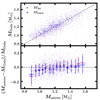 |
Fig. 6. One-to-one comparison of Gaia and asteroseismic mass scales (top) and the fractional differences (bottom; with binned medians and uncertainties on the median). The mean agreement between the different mass scales, the Gaia mass scales Mνmax and MΔν, and the asteroseismic mass scale, Mastero, are consistent to within the uncertainties on the mean (1.5%, respectively). |
At this stage, we found that the scatter in stellar masses and radii – when compared to Gaia data – was smaller than the uncertainties obtained from propagating errors in Δν and νmax. To address this discrepancy, we decided to rescale our error bars. We divided the sample into bins of mass (or radius), within which we computed the scatter of the fractional differences (see Figs. 5, 6). We then rescaled the uncertainties in the masses (or radii) for each bin so that the mean relative uncertainty matched the observed scatter in the fractional differences. On average this has decreased the uncertainty on the radius by a factor of 4 and decreased the uncertainty on the mass by a factor of 2.
5. Discussion
Stars near the Kepler Nyquist frequency are particularly interesting for constraining stellar models. As we show in the HR diagrams Fig. 7, these stars sit in the curve where stars turn from moving horizontally across the subgiant branch to moving vertically up the RGB. Our sample spans a range of metallicities (−0.4 to +0.2 dex) and masses (0.8 M⊙ to 1.6 M⊙). When we compare the measured temperatures and luminosities of these stars to the predictions of stellar models, we find that the stars in general are well matched to the models as a function of mass and metallicity, consistent with previous results (e.g., Grusnis et al. 2025). Such agreement is not generally found for more evolved giants (e.g. Tayar et al. 2017). This agreement suggests that masses and ages estimated from temperature and luminosity are likely to be reliable in this regime, providing an opportunity for large galactic archaeology studies based on Gaia data (e.g., Xiang & Rix 2022; Nataf et al. 2024).
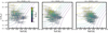 |
Fig. 7. HR diagram color-coded by νmax+Gaia mass and binned by metallicity. Luminosity was computed from Gaia radii. MIST evolutionary tracks for stars with masses between 0.8 M⊙ and 1.6 M⊙ and metallicities equal to the central metallicity of each bin are shown for reference. The sample spans an interesting range in mass and age as well as metallicity so that the FDU can be studied (the clump is visible in the MIST tracks as kinks above the locus of the sample); see Fig. 8. |
The stars in this sample also cover the moment in which stars undergo the FDU. During this process, the convective envelope deepens into a region that has previously undergone the CNO cycle, and thus has a different balance of carbon and nitrogen than the stellar surface. This processed material is mixed up to the stellar surface, and changes the observed abundance ratios once it occurs. How much the ratios change depends on both the depth of the dredge-up and the amount of CNO burning that happened in that zone, and should therefore depend most on the mass and somewhat on the metallicity of the star. We show in Fig. 8 the observed ratio of the carbon to nitrogen [C/N] as a function of surface gravity, compared to the predicted evolution in stellar models of various masses. In general, the location of the dredge-up seems to be close to correct, but the depth of the dredge-up, and its mass dependence in the data do not match the predictions of models very well. This could be due to errors in the assumed model physics, or to errors in the observed abundance scale, which is notoriously difficult to calibrate and varies between surveys (Jönsson et al. 2018). This zero-point offset is also observed in Cao & Pinsonneault (2025) – for example, in Fig. 6, where it is argued that these probably stem from the APOGEE data itself or from the assumption that trends in carbon and nitrogen abundance in subgiants (Roberts et al. 2024) – and the birth trends of RGB stars are the same. In either case, this sample could prove uniquely valuable for constraining the mixing occurring during the FDU, expanding the work done by Roberts et al. (2024).
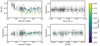 |
Fig. 8. Δ[C/N], i.e., change in the surface carbon-to-nitrogen abundance ratio since birth vs. the seismic log(g) and residuals as a function of log(g), mass, and metallicity for stars with metallicities of −0.1 < [Fe/H]< 0.1 and masses of 1.2M⊙ < M < 1.4 M⊙ found in the present work (marked with opaque dots) along with stars found in the APOKASC-3 catalog (marked with semitransparent circles) (Pinsonneault et al. 2025). The stars flagged as being part of the RC in APOKASC-3 were removed from this figure. Evolutionary tracks from Cao & Pinsonneault (2025) with solar metallicity are overlaid on top of the data. The error bars on mass and metallicity have been shrunk by factors of 20 and 10, respectively, in order to improve readability of the graph. Stars evolve from left to right in the left panels of the plot. We note that the end of the dredge-up is expected to be between log g = 2.9 and log g = 3.1 (see Fig. 4 of Cao & Pinsonneault 2025); hence, all our stars are undergoing the FDU. |
This work successfully reproduces, at a qualitative level, the population trends observed in Pinsonneault et al. (2025), as is illustrated in Figs. 9 and 10. In particular, Fig. 10 reveals the same population effect as Fig. 18 in Pinsonneault et al. (2025); namely, the absence of low-metallicity, low-mass stars in our sample.
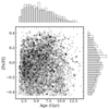 |
Fig. 9. Metallicity vs. age: The open black circles and black-outlined histograms represent the sample from this paper with available APOGEE spectra, while the semitransparent circles and gray histograms correspond to data from the APOKASC-3 paper (Pinsonneault et al. 2025). Ages outside the range of 0 to 14 Gyr have been excluded. The stars flagged as being part of the RC in APOKASC-3 were removed from this figure. |
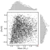 |
Fig. 10. Mass vs. [Fe/H]: The open black circles and black-outlined histograms represent the sample from this paper with available APOGEE spectra, while the semitransparent circles and gray histograms correspond to data from the APOKASC-3 paper (Pinsonneault et al. 2025). The stars flagged as being part of the RC in APOKASC-3 were removed from this figure. |
While broadly similar, the distributions of mass, age, and metallicity in our sample and the APOKASC-3 catalog exhibit some differences:
-
A noticeable underrepresentation of stars aged between 9 and 10.5 Gyr. This is likely due to an underrepresentation of alpha-rich stars in our sample compared to the APOKASC-3 one. Indeed, plotting the same figure as Fig. 9 with only alpha-poor stars gets rid of this effect. However, given that the age uncertainties are typically larger than 2 Gyr, the statistical significance of the dip observed in the histogram remains uncertain.
-
Fewer stars with low [Fe/H] compared to the APOKASC-3 sample.
-
A higher number of stars with [Fe/H] between 0.1 and 0.2 than in the APOKASC-3 catalog.
-
A lower number of low-mass stars compared to APOKASC-3.
These differences likely stem from the smaller size of our sample relative to the APOKASC-3 catalog.
6. Conclusion
In this paper, we developed part of the PyA2Z pipeline, a revised Python version of the A2Z pipeline. In addition to the old pipeline, PyA2Z flags stars that are likely to be super-Nyquist. This methodology relies on the seismic scaling relations, where the measured Δν is compared with the νmax obtained below νNyq and with νmax from the mirrored PSD.
We have demonstrated that PyA2Z is able to identify and correctly measure stars whose oscillations are close to or just above the Nyquist frequency. We lay out a method of distinguishing real from mirrored modes by identifying the radial-quadrupole structure in the echelle diagram that follows the seismic scaling relation δν0, 2(Δν) calibrated for RGs.
Applying these methods to a sample of 2 065 Kepler targets yields a new asteroseismic catalog of 285 super-Nyquist stars as well as 168 close-to-Nyquist stars for which we give the global seismic parameters Δν and νmax. Our results expand the known sample of super-Nyquist oscillators by a factor of 7.
Using a grid of stellar models computed with GARSTEC, we obtained the masses, radii, and ages of 892 stars. Our sample covers a range in mass from 0.8 to 1.6 M⊙ and in metallicity from -0.4 to +0.2 dex. Comparisons of the measured temperatures and luminosities of our set of stars with stellar models show good agreement in this evolutionary phase, suggesting that mass and age estimates from temperature and luminosity are reliable in this regime.
The study of the dredge-up phase shows that its timing matches model predictions, but the depth and mass dependence do not align well. This could be due to uncertainties in model physics or calibration issues in observed abundance scales. Our study qualitatively reproduces trends observed in previous works but reveals key differences when compared to the APOKASC-3 catalog. Specifically, our sample shows an underrepresentation of stars aged between 9 and 10.5 Gyr, as well as a lower fraction of metal-poor stars. Conversely, we observe a higher proportion of stars with a slightly enhanced metallicity ([Fe/H] = 0.1–0.2) and a lower number of low-mass stars relative to APOKASC-3. These discrepancies are likely a consequence of our smaller sample size, which may introduce selection effects when compared to the larger APOKASC-3 dataset.
Gathering more data in the FDU domain will enable a meaningful test of stellar theory. In particular, Li destruction during this phase is a sensitive test of envelope overshooting, which is commonly invoked to explain the mismatch between the observed and predicted RGB bump. Existing data are in clear tension with stellar evolution models (Cao & Pinsonneault 2025), but the overlap between seismic masses and Li surveys has been limited. The southern GALAH survey, in particular, did not observed the Kepler fields, so we cannot test this directly with our sample. TESS or K2, however, are much more promising in this regard.
We also expect that current and future missions will continue to increase the number of stars in this parameter space that are available for study. In the TESS mission, the full frame image cadence decreased to 10 minutes and 3 minutes during the two extended missions. The PLAnetary Transits and Oscillations of stars (PLATO, Rauer et al. 2014) mission should also allow for a large number of detections of solar-like oscillations in the subgiant phase given the yield predictions (Goupil et al. 2024). However, the 1440 day duration of the Kepler mission continues to be unmatched, and so we expect these near and super-Nyquist stars to remain a valuable addition to the literature for years to come.
Data availability
The data from Tables 2, 3 as well as the data described in Table E.1 are available at the CDS via https://cdsarc.cds.unistra.fr/viz-bin/cat/J/A+A/702/A144.
Acknowledgments
This paper includes data collected by the Kepler mission and obtained from the MAST data archive at the Space Telescope Science Institute (STScI). Funding for the Kepler mission is provided by the NASA Science Mission Directorate. STScI is operated by the Association of Universities for Research in Astronomy, Inc., under NASA contract NAS 5–26555. R.A.G. acknowledges the support from the GOLF and PLATO Centre National D’Études Spatiales grants. S.M. acknowledges support by the Spanish Ministry of Science and Innovation with the grant number PID2019-107061GB-C66, and through AEI under the Severo Ochoa Centres of Excellence Programme 2020–2023 (CEX2019-000920-S). B.L. thanks École Normale Supérieure Paris-Saclay (France) for its stipend that made possible to fund a long stay abroad. SM, DHG, DGR, and RAG acknowledge support from the Spanish Ministry of Science and Innovation with the grant no. PID2023-149439NB-C41. PGB acknowledges support by the Spanish Ministry of Science and Innovation with the Ramón y Cajal fellowship number RYC-2021-033137-I and the number MRR4032204. PGB, DHG, DGR, and RAG acknowledge support from the Spanish Ministry of Science and Innovation with the grant no. PID2023-146453NB-100 (PLAtoSOnG). AS acknowledges support by the Spanish Ministry of Science, Innovation and Universities through the grant PID2023-149918NB-I00 and the program Unidad de Excelencia María de Maeztu CEX2020-001058-M, and Generalitat de Catalunya through grant 2021-SGR-1526. MHP acknowledges support from NASA grant 80NSSC24K0637. MHP acknowledges support from the Fundación Occident and the Instituto de Astrofísica de Canarias under the Visiting Researcher Programme 2022-2025 agreed between both institutions. DGR acknowledges support from the Juan de la Cierva program under contract JDC2022-049054-I. DHG acknowledges the support of a fellowship from “la Caixa” Foundation (ID 100010434). The fellowship code is LCF/BQ/DI23/11990068. Software: AstroPy (Astropy Collaboration 2013, 2018), Matplotlib (Hunter 2007), NumPy (Harris et al. 2020), SciPy (Virtanen et al. 2020)
References
- Abdurro’uf, Accetta, K., Aerts, C., et al. 2022, ApJS, 259, 35 [NASA ADS] [CrossRef] [Google Scholar]
- Ahumada, R., Allende Prieto, C., Almeida, A., et al. 2020, ApJS, 249, 3 [NASA ADS] [CrossRef] [Google Scholar]
- Anders, F., Chiappini, C., Rodrigues, T. S., et al. 2016, A&A, 597, A30 [Google Scholar]
- Andrae, R., Rix, H.-W., & Chandra, V. 2023, ApJS, 267, 8 [NASA ADS] [CrossRef] [Google Scholar]
- Astropy Collaboration (Robitaille, T. P., et al.) 2013, A&A, 558, A33 [NASA ADS] [CrossRef] [EDP Sciences] [Google Scholar]
- Astropy Collaboration (Price-Whelan, A. M. et al.) 2018, AJ, 156, 123 [Google Scholar]
- Baglin, A., Auvergne, M., Boisnard, L., et al. 2006, in 36th COSPAR Scientific Assembly, COSPAR, Plenary Meeting, 36, 3749 [Google Scholar]
- Ballot, J., Gizon, L., Samadi, R., et al. 2011, A&A, 530, A97 [NASA ADS] [CrossRef] [EDP Sciences] [Google Scholar]
- Basinger, C., Pinsonneault, M., Bastelberger, S. T., Gaudi, B. S., & Domagal-Goldman, S. D. 2024, MNRAS, 534, 2968 [NASA ADS] [CrossRef] [Google Scholar]
- Beaton, R. L., Oelkers, R. J., Hayes, C. R., et al. 2021, AJ, 162, 302 [NASA ADS] [CrossRef] [Google Scholar]
- Beck, P. G., Montalban, J., Kallinger, T., et al. 2012, Nature, 481, 55 [Google Scholar]
- Beck, P. G., Kallinger, T., Pavlovski, K., et al. 2018, A&A, 612, A22 [NASA ADS] [CrossRef] [EDP Sciences] [Google Scholar]
- Benomar, O., Baudin, F., Campante, T. L., et al. 2009, A&A, 507, L13 [NASA ADS] [CrossRef] [EDP Sciences] [Google Scholar]
- Berger, T. A., Huber, D., Gaidos, E., & van Saders, J. L. 2018, ApJ, 866, 99 [NASA ADS] [CrossRef] [Google Scholar]
- Blanton, M. R., Bershady, M. A., Abolfathi, B., et al. 2017, AJ, 154, 28 [Google Scholar]
- Borucki, W. J., Koch, D., Basri, G., et al. 2010, Science, 327, 977 [Google Scholar]
- Bovy, J., Rix, H.-W., Green, G. M., Schlafly, E. F., & Finkbeiner, D. P. 2016, ApJ, 818, 130 [Google Scholar]
- Breton, S. N., García, R. A., Ballot, J., Delsanti, V., & Salabert, D. 2022, A&A, 663, A118 [NASA ADS] [CrossRef] [EDP Sciences] [Google Scholar]
- Breton, S. N., García, R. A., Ballot, J., Delsanti, V., & Salabert, D. 2023, apollinaire: Helioseismic and asteroseismic peakbagging frameworks, Astrophysics Source Code Library [record ascl:2306.022] [Google Scholar]
- Brown, T. M. 1991, ApJ, 371, 396 [NASA ADS] [CrossRef] [Google Scholar]
- Cao, K., & Pinsonneault, M. H. 2025, arXiv e-prints [arXiv:2501.14867] [Google Scholar]
- Carrasco, J. M., Weiler, M., Jordi, C., et al. 2021, A&A, 652, A86 [NASA ADS] [CrossRef] [EDP Sciences] [Google Scholar]
- Casagrande, L., Ramírez, I., Meléndez, J., Bessell, M., & Asplund, M. 2010, A&A, 512, A54 [NASA ADS] [CrossRef] [EDP Sciences] [Google Scholar]
- Chaplin, W. J., Elsworth, Y., Davies, G. R., et al. 2014, MNRAS, 445, 946 [NASA ADS] [CrossRef] [Google Scholar]
- Chen, T., & Guestrin, C. 2016, arXiv e-prints [arXiv:1603.02754] [Google Scholar]
- Choi, J., Dotter, A., Conroy, C., et al. 2016, ApJ, 823, 102 [Google Scholar]
- Christensen-Dalsgaard, J. 1984, in Space Research in Stellar Activity and Variability, eds. A. Mangeney, & F. Praderie, 11 [Google Scholar]
- Corsaro, E., & De Ridder, J. 2014, A&A, 571, A71 [NASA ADS] [CrossRef] [EDP Sciences] [Google Scholar]
- Corsaro, E., Stello, D., Huber, D., et al. 2012, ApJ, 757, 190 [Google Scholar]
- Davies, G. R., Chaplin, W. J., Farr, W. M., et al. 2015, MNRAS, 446, 2959 [CrossRef] [Google Scholar]
- Davies, G. R., Silva Aguirre, V., Bedding, T. R., et al. 2016, MNRAS, 456, 2183 [Google Scholar]
- De Ridder, J., Barban, C., Baudin, F., et al. 2009, Nature, 459, 398 [Google Scholar]
- Deheuvels, S., García, R. A., Chaplin, W. J., et al. 2012, ApJ, 756, 19 [Google Scholar]
- Deheuvels, S., Doğan, G., Goupil, M. J., et al. 2014, A&A, 564, A27 [NASA ADS] [CrossRef] [EDP Sciences] [Google Scholar]
- Dotter, A. 2016, ApJS, 222, 8 [Google Scholar]
- Drimmel, R., Cabrera-Lavers, A., & López-Corredoira, M. 2003, A&A, 409, 205 [NASA ADS] [CrossRef] [EDP Sciences] [Google Scholar]
- Eisenstein, D. J., Weinberg, D. H., Agol, E., et al. 2011, AJ, 142, 72 [Google Scholar]
- Gaia Collaboration (Vallenari, A., et al.) 2023, A&A, 674, A1 [NASA ADS] [CrossRef] [EDP Sciences] [Google Scholar]
- García Pérez, A. E., Allende Prieto, C., Holtzman, J. A., et al. 2016, AJ, 151, 144 [Google Scholar]
- García, R. A., & Ballot, J. 2019, Liv. Rev. Sol. Phys., 16, 4 [Google Scholar]
- García, R. A., Hekker, S., Stello, D., et al. 2011, MNRAS, 414, L6 [NASA ADS] [CrossRef] [Google Scholar]
- García, R. A., Mathur, S., Pires, S., et al. 2014a, A&A, 568, A10 [Google Scholar]
- García, R. A., Pérez Hernández, F., Benomar, O., et al. 2014b, A&A, 563, A84 [NASA ADS] [CrossRef] [EDP Sciences] [Google Scholar]
- García, R. A., Palakkatharappil, D. B., Bugnet, L., et al. 2024a, in 8th TESS/15th Kepler Asteroseismic Science Consortium Workshop, 123 [Google Scholar]
- García, R. A., Palakkatharappil, D. B., Mathur, S., et al. 2024b, in TESS Science Conference III, 32 [Google Scholar]
- Gilliland, R. L., Jenkins, J. M., Borucki, W. J., et al. 2010, ApJ, 713, L160 [Google Scholar]
- Godoy-Rivera, D., Tayar, J., Pinsonneault, M. H., et al. 2021, ApJ, 915, 19 [NASA ADS] [CrossRef] [Google Scholar]
- Godoy-Rivera, D., Mathur, S., García, R. A., et al. 2025, A&A, 696, A243 [Google Scholar]
- Goldreich, P., & Keeley, D. A. 1977, ApJ, 212, 243 [NASA ADS] [CrossRef] [Google Scholar]
- González Hernández, J. I., & Bonifacio, P. 2009, A&A, 497, 497 [Google Scholar]
- González-Cuesta, L., Mathur, S., García, R. A., et al. 2023, A&A, 674, A106 [NASA ADS] [CrossRef] [EDP Sciences] [Google Scholar]
- Goupil, M. J., Catala, C., Samadi, R., et al. 2024, A&A, 683, A78 [NASA ADS] [CrossRef] [EDP Sciences] [Google Scholar]
- Green, G. M., Schlafly, E., Zucker, C., Speagle, J. S., & Finkbeiner, D. 2019, ApJ, 887, 93 [NASA ADS] [CrossRef] [Google Scholar]
- Grevesse, N., & Sauval, A. J. 1998, Space Sci. Rev., 85, 161 [Google Scholar]
- Grusnis, S., Tayar, J., & Godoy-Rivera, D. 2025, ApJ, Arxiv e-prints [arXiv:2509.12513] [Google Scholar]
- Gunn, J. E., Siegmund, W. A., Mannery, E. J., et al. 2006, AJ, 131, 2332 [NASA ADS] [CrossRef] [Google Scholar]
- Harris, C. R., Millman, K. J., van der Walt, S. J., et al. 2020, Nature, 585, 357 [NASA ADS] [CrossRef] [Google Scholar]
- Harvey, J. 1985, in Future Missions in Solar, Heliospheric& Space Plasma Physics, eds. E. Rolfe, & B. Battrick, ESA Spec. Pub., 235, 199 [NASA ADS] [Google Scholar]
- Hatt, E., Nielsen, M. B., Chaplin, W. J., et al. 2023, A&A, 669, A67 [NASA ADS] [CrossRef] [EDP Sciences] [Google Scholar]
- Hekker, S., Gilliland, R. L., Elsworth, Y., et al. 2011, MNRAS, 414, 2594 [Google Scholar]
- Hermes, J. J., Gänsicke, B. T., Kawaler, S. D., et al. 2017, ApJS, 232, 23 [Google Scholar]
- Hon, M., Huber, D., Kuszlewicz, J. S., et al. 2021, ApJ, 919, 131 [NASA ADS] [CrossRef] [Google Scholar]
- Howell, S. B., Sobeck, C., Haas, M., et al. 2014, PASP, 126, 398 [Google Scholar]
- Huang, C. X., Vanderburg, A., Pál, A., et al. 2020a, Res. Notes Am. Astron. Soc., 4, 204 [Google Scholar]
- Huang, C. X., Vanderburg, A., Pál, A., et al. 2020b, Res. Notes Am. Astron. Soc., 4, 206 [Google Scholar]
- Huber, D., Bedding, T. R., Stello, D., et al. 2010, ApJ, 723, 1607 [NASA ADS] [CrossRef] [Google Scholar]
- Huber, D., Bedding, T. R., Stello, D., et al. 2011, ApJ, 743, 143 [Google Scholar]
- Huber, D., Silva Aguirre, V., Matthews, J. M., et al. 2014, ApJS, 211, 2 [NASA ADS] [CrossRef] [Google Scholar]
- Huber, D., White, T. R., Metcalfe, T. S., et al. 2022, AJ, 163, 79 [NASA ADS] [CrossRef] [Google Scholar]
- Hunter, J. D. 2007, Comput. Sci. Eng., 9, 90 [NASA ADS] [CrossRef] [Google Scholar]
- Iben, I., Jr 1965, ApJ, 142, 1447 [NASA ADS] [CrossRef] [Google Scholar]
- Jenkins, J. M., Caldwell, D. A., Chandrasekaran, H., et al. 2010, ApJ, 713, L120 [Google Scholar]
- Jönsson, H., Allende Prieto, C., Holtzman, J. A., et al. 2018, AJ, 156, 126 [Google Scholar]
- Kallinger, T., De Ridder, J., Hekker, S., et al. 2014, A&A, 570, A41 [NASA ADS] [CrossRef] [EDP Sciences] [Google Scholar]
- Karakas, A. I., & Lattanzio, J. C. 2014, PASA, 31, e030 [NASA ADS] [CrossRef] [Google Scholar]
- Kjeldsen, H., & Bedding, T. R. 1995, A&A, 293, 87 [NASA ADS] [Google Scholar]
- Kumar, P., Franklin, J., & Goldreich, P. 1988, ApJ, 328, 879 [Google Scholar]
- Kunimoto, M., Tey, E., Fong, W., Hesse, K., & Shporer, A. 2022, Res. Notes Am. Astron. Soc., 6, 235 [Google Scholar]
- Kurucz, R. L. 1970, SAO Spec. Rep., 309 [Google Scholar]
- Kurucz, R. L. 1993, in IAU Colloq. 138: Peculiar versus Normal Phenomena in A-type and Related Stars, eds. M. M. Dworetsky, F. Castelli, & R. Faraggiana, ASP Conf. Ser., 44, 87 [Google Scholar]
- Li, G., Deheuvels, S., Ballot, J., & Lignières, F. 2022, Nature, 610, 43 [NASA ADS] [CrossRef] [Google Scholar]
- Lindegren, L., Bastian, U., Biermann, M., et al. 2021a, A&A, 649, A4 [EDP Sciences] [Google Scholar]
- Lindegren, L., Klioner, S. A., Hernández, J., et al. 2021b, A&A, 649, A2 [EDP Sciences] [Google Scholar]
- Lund, M. N., Silva Aguirre, V., Davies, G. R., et al. 2017, ApJ, 835, 172 [Google Scholar]
- Lund, M. N., Basu, S., Bieryla, A., et al. 2024, A&A, 688, A13 [NASA ADS] [CrossRef] [EDP Sciences] [Google Scholar]
- Majewski, S. R., Schiavon, R. P., Frinchaboy, P. M., et al. 2017, AJ, 154, 94 [NASA ADS] [CrossRef] [Google Scholar]
- Marshall, D. J., Robin, A. C., Reylé, C., Schultheis, M., & Picaud, S. 2006, A&A, 453, 635 [NASA ADS] [CrossRef] [EDP Sciences] [Google Scholar]
- Martig, M., Fouesneau, M., Rix, H.-W., et al. 2016, MNRAS, 456, 3655 [NASA ADS] [CrossRef] [Google Scholar]
- Mathur, S., Garcia, R. A., Régulo, C., et al. 2010, A&A, 511, A46 [NASA ADS] [CrossRef] [EDP Sciences] [Google Scholar]
- Mathur, S., Hekker, S., Trampedach, R., et al. 2011, ApJ, 741, 119 [Google Scholar]
- Mathur, S., García, R. A., Huber, D., et al. 2016, ApJ, 827, 50 [NASA ADS] [CrossRef] [Google Scholar]
- Mathur, S., Huber, D., Batalha, N. M., et al. 2017, ApJS, 229, 30 [NASA ADS] [CrossRef] [Google Scholar]
- Mathur, S., García, R. A., Breton, S., et al. 2022, A&A, 657, A31 [NASA ADS] [CrossRef] [EDP Sciences] [Google Scholar]
- Mazumdar, A., Monteiro, M. J. P. F. G., Ballot, J., et al. 2012, Astron. Nachr., 333, 1040 [NASA ADS] [Google Scholar]
- Mazumdar, A., Monteiro, M. J. P. F. G., Ballot, J., et al. 2014, ApJ, 782, 18 [NASA ADS] [CrossRef] [Google Scholar]
- Metcalfe, T. S., van Saders, J. L., Huber, D., et al. 2024, ApJ, 974, 31 [Google Scholar]
- Mosser, B., Belkacem, K., Goupil, M., et al. 2010, A&A, 517, A22 [NASA ADS] [CrossRef] [EDP Sciences] [Google Scholar]
- Mosser, B., Elsworth, Y., Hekker, S., et al. 2012, A&A, 537, A30 [NASA ADS] [CrossRef] [EDP Sciences] [Google Scholar]
- Mosser, B., Michel, E., Samadi, R., et al. 2019, A&A, 622, A76 [NASA ADS] [CrossRef] [EDP Sciences] [Google Scholar]
- Murphy, S. J., Shibahashi, H., & Kurtz, D. W. 2013, MNRAS, 430, 2986 [NASA ADS] [CrossRef] [Google Scholar]
- Nataf, D. M., Schlaufman, K. C., Reggiani, H., & Hahn, I. 2024, ApJ, 976, 87 [Google Scholar]
- Ness, M., Hogg, D. W., Rix, H. W., et al. 2016, ApJ, 823, 114 [NASA ADS] [CrossRef] [Google Scholar]
- Ong, J. M. J., Basu, S., Lund, M. N., et al. 2021, ApJ, 922, 18 [NASA ADS] [CrossRef] [Google Scholar]
- Paxton, B., Bildsten, L., Dotter, A., et al. 2011, ApJS, 192, 3 [Google Scholar]
- Paxton, B., Cantiello, M., Arras, P., et al. 2013, ApJS, 208, 4 [Google Scholar]
- Paxton, B., Marchant, P., Schwab, J., et al. 2015, ApJS, 220, 15 [Google Scholar]
- Pinsonneault, M. H., Elsworth, Y. P., Tayar, J., et al. 2018, ApJS, 239, 32 [Google Scholar]
- Pinsonneault, M. H., Zinn, J. C., Tayar, J., et al. 2025, ApJS, 276, 69 [NASA ADS] [CrossRef] [Google Scholar]
- Pires, S., Mathur, S., García, R. A., et al. 2015, A&A, 574, A18 [NASA ADS] [CrossRef] [EDP Sciences] [Google Scholar]
- Rauer, H., Catala, C., Aerts, C., et al. 2014, Exp. Astron., 38, 249 [Google Scholar]
- Ricker, G. R., Winn, J. N., Vanderspek, R., et al. 2014, SPIE Conf. Ser., 9143, 20 [Google Scholar]
- Roberts, J. D., Pinsonneault, M. H., Johnson, J. A., et al. 2024, MNRAS, 530, 149 [Google Scholar]
- Rybizki, J., Green, G. M., Rix, H.-W., et al. 2022, MNRAS, 510, 2597 [NASA ADS] [CrossRef] [Google Scholar]
- Salaris, M., Chieffi, A., & Straniero, O. 1993, ApJ, 414, 580 [NASA ADS] [CrossRef] [Google Scholar]
- Salaris, M., Pietrinferni, A., Piersimoni, A. M., & Cassisi, S. 2015, A&A, 583, A87 [NASA ADS] [CrossRef] [EDP Sciences] [Google Scholar]
- Santos, Â. R. G., García, R. A., Mathur, S., et al. 2019, ApJS, 244, 21 [NASA ADS] [CrossRef] [Google Scholar]
- Santos, Â. R. G., Breton, S. N., Mathur, S., & García, R. A. 2021, ApJS, 255, 17 [NASA ADS] [CrossRef] [Google Scholar]
- Serenelli, A. M., Bergemann, M., Ruchti, G., & Casagrande, L. 2013, MNRAS, 429, 3645 [NASA ADS] [CrossRef] [Google Scholar]
- Serenelli, A., Johnson, J., Huber, D., et al. 2017, ApJS, 233, 23 [Google Scholar]
- Sharma, S., Stello, D., Bland-Hawthorn, J., Huber, D., & Bedding, T. R. 2016, ApJ, 822, 15 [Google Scholar]
- Silva Aguirre, V., Lund, M. N., Antia, H. M., et al. 2017, ApJ, 835, 173 [Google Scholar]
- Stello, D., & Sharma, S. 2022, Res. Notes Am. Astron. Soc., 6, 168 [Google Scholar]
- Stello, D., Chaplin, W., Basu, S., Elsworth, Y., & Bedding, T. 2009, MNRAS, 400, L80 [CrossRef] [Google Scholar]
- Stello, D., Huber, D., Bedding, T. R., et al. 2013, ApJ, 765, L41 [CrossRef] [Google Scholar]
- Stello, D., Huber, D., Sharma, S., et al. 2015, ApJ, 809, L3 [NASA ADS] [CrossRef] [Google Scholar]
- Stello, D., Zinn, J., Elsworth, Y., et al. 2017, ApJ, 835, 83 [NASA ADS] [CrossRef] [Google Scholar]
- Tassoul, M. 1980, ApJS, 43, 469 [Google Scholar]
- Tayar, J., Somers, G., Pinsonneault, M. H., et al. 2017, ApJ, 840, 17 [NASA ADS] [CrossRef] [Google Scholar]
- Virtanen, P., Gommers, R., Oliphant, T. E., et al. 2020, Nat. Methods, 17, 261 [Google Scholar]
- Weiss, A., & Schlattl, H. 2008, Ap&SS, 316, 99 [CrossRef] [Google Scholar]
- Wilson, J. C., Hearty, F. R., Skrutskie, M. F., et al. 2019, PASP, 131, 055001 [NASA ADS] [CrossRef] [Google Scholar]
- Xiang, M., & Rix, H.-W. 2022, Nature, 603, 599 [NASA ADS] [CrossRef] [Google Scholar]
- York, D. G., Adelman, J., Anderson, J. E., Jr, et al. 2000, AJ, 120, 1579 [Google Scholar]
- Yu, J., Huber, D., Bedding, T. R., et al. 2016, MNRAS, 463, 1297 [Google Scholar]
- Yu, J., Huber, D., Bedding, T. R., et al. 2018, ApJS, 236, 42 [NASA ADS] [CrossRef] [Google Scholar]
- Zasowski, G., Johnson, J. A., Frinchaboy, P. M., et al. 2013, AJ, 146, 81 [NASA ADS] [CrossRef] [Google Scholar]
- Zasowski, G., Cohen, R. E., Chojnowski, S. D., et al. 2017, AJ, 154, 198 [Google Scholar]
- Zinn, J. C., Huber, D., Pinsonneault, M. H., & Stello, D. 2017, ApJ, 844, 166 [Google Scholar]
- Zinn, J. C., Pinsonneault, M. H., Huber, D., et al. 2019, ApJ, 885, 166 [Google Scholar]
- Zinn, J. C., Stello, D., Elsworth, Y., et al. 2020, ApJS, 251, 23 [NASA ADS] [CrossRef] [Google Scholar]
- Zinn, J. C., Stello, D., Elsworth, Y., et al. 2022, ApJ, 926, 191 [NASA ADS] [CrossRef] [Google Scholar]
Appendix A: Flowchart
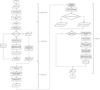 |
Fig. A.1. Flowchart of the method used. |
Appendix B: Scaling relation used for this article
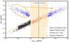 |
Fig. B.1. Stars recovered in this work, shown along with the scaling relation adopted in our analysis (orange dashed line). The vertical green line marks the Nyquist frequency. To the left of this line, sub-Nyquist stars are shown in black and super-Nyquist stars, initially misidentified with a frequency νmax = νmax,sub, are shown in blue. To the right of the Nyquist frequency, the same super-Nyquist stars are plotted in blue with their corrected values νmax = 2 × νNyq − νmax,sub. Stars located near the Nyquist frequency, where mode overlap is significant, are shown in red within the yellow shaded region. |
Appendix C: Apodization effects
When a point on a light curve is measured, the star’s luminosity flux is integrated on  min. Let us introduce the function that represents the light received from the star by the sensor of Kepler at a time t: L : t ↦ L(t) as well as the function V that represents the discrete light curve given by Kepler with a point every sampling period. Is also introduced the function
Then one point of the light curve at τ corresponds to:
 (C.1)
(C.1)
The symbol refers to the convolution product. This means that the light curve can be expressed as:
 (C.2)
(C.2)
where T is the Dirac comb function of period T. Hence the PSD of the light curves is:
\right|^2\times {{\,\mathrm{sinc}\,}}^2(\pi T_{\mathrm{samp} }\nu )\quad .\end{aligned} $$](/articles/aa/full_html/2025/10/aa55167-25/aa55167-25-eq45.gif) (C.3)
(C.3)
With ℱ[L] the Fourier transform of the function L. Besides by definition νsamp = 2νNyq. Hence the apodization effect is due to the term  .
.
That apodization leads to a deformation of the Gaussian envelope of the modes that can cause biases to the measure of νmax since the modes’ amplitudes are no longer symmetrically distributed.
Appendix D: Analysis of TESS data
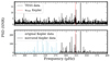 |
Fig. D.1. PSD of TIC 123498033/KIC 8279949 as observed by Kepler LC and TESS. |
We analyzed TESS light curves using the Simple Aperture Photometry (SAP) flux extracted from QLP data. These fluxes were corrected with PyTADACS, an adaptation of the Kepler Asteroseismic Data Calibration Software (KADACS; García et al. 2011) specifically tailored for TESS observations. PyTADACS, currently under development, provides enhanced calibration for TESS data (see García et al. 2024b,a, for further details). From the 2 104 Kepler targets analyzed in this work, we only found 1 140 available in TESS QLP data up to sector 80. After applying PyA2Z, only 9 stars had detectable oscillations. Results are reported in Table D.1.
Comparison of TESS and Kepler retrieved global seismic parameters.
Appendix E: Columns of the table published with this article
Columns included in the final table.
1440 days being the duration of the Kepler mission.
[Fe/H]corr = [Fe/H] + 0.625 [α/Fe] is used to account for alpha enhancement, as the grid of stellar models uses a solar-scaled composition. This is the same correction as the one adopted in Pinsonneault et al. (2025) and is quantitatively similar, to other corrections, such as the one from Salaris et al. (1993).
All Tables
All Figures
|
Fig. 1. Power spectral density (PSD) of two simulated stars in units of the signal-to-noise ratio (SNR) as a function of frequency. Panel (a): Star with modes close to νNyq at the right edge of the frequency range. The true modes are in orange and the mirrored modes in black. Panel (b): Star with super-Nyquist modes where only the folded modes are observed between 0 μHz and νNyq. |
| In the text | |
|
Fig. 2. PSD of the star KIC 8179973 and estimate of its background with a median filter. |
| In the text | |
|
Fig. 3. (a) PSD of the Kepler star KIC 8179973 on which a sliding box (shaded pink area) was used to compute the PS2 (inset) with Γ = 2 and filtered as explained in Section 3.1.1. (b) The red line is the averaged filtered PS2 normalized to its maximum value as a function of the center of the sliding windows. The dashed black line is the Gaussian fit. |
| In the text | |
|
Fig. 4. (a) Synthesized PSD of the ℓ = 0, 2 modes of a star with νmax = 275 μHz. The black modes are the true modes, whereas the blue modes are those observed because of the undersampling: they are the black modes mirrored around νNyq. Each box of width Δν matches to one line of the echelle diagram shown in panel (b) along with its collapse in (c). In (b), the ridges due to the true modes are annotated in black, whereas those annotated in blue are due to the shadow modes. In (c) the peaks due to the mirrored modes are marked with a vertical dashed blue line and the peaks due to the true modes are marked with a vertical dotted black line. |
| In the text | |
|
Fig. 5. One-to-one comparison of Gaia and asteroseimsic radius scales (top) and the fractional differences (bottom; with binned medians and uncertainties on the median). The two show excellent agreement (to within 0.9% on average), which demonstrates the accuracy of the asteroseismic analysis here and of the asteroseismic radius scale in the subgiant regime. |
| In the text | |
|
Fig. 6. One-to-one comparison of Gaia and asteroseismic mass scales (top) and the fractional differences (bottom; with binned medians and uncertainties on the median). The mean agreement between the different mass scales, the Gaia mass scales Mνmax and MΔν, and the asteroseismic mass scale, Mastero, are consistent to within the uncertainties on the mean (1.5%, respectively). |
| In the text | |
|
Fig. 7. HR diagram color-coded by νmax+Gaia mass and binned by metallicity. Luminosity was computed from Gaia radii. MIST evolutionary tracks for stars with masses between 0.8 M⊙ and 1.6 M⊙ and metallicities equal to the central metallicity of each bin are shown for reference. The sample spans an interesting range in mass and age as well as metallicity so that the FDU can be studied (the clump is visible in the MIST tracks as kinks above the locus of the sample); see Fig. 8. |
| In the text | |
|
Fig. 8. Δ[C/N], i.e., change in the surface carbon-to-nitrogen abundance ratio since birth vs. the seismic log(g) and residuals as a function of log(g), mass, and metallicity for stars with metallicities of −0.1 < [Fe/H]< 0.1 and masses of 1.2M⊙ < M < 1.4 M⊙ found in the present work (marked with opaque dots) along with stars found in the APOKASC-3 catalog (marked with semitransparent circles) (Pinsonneault et al. 2025). The stars flagged as being part of the RC in APOKASC-3 were removed from this figure. Evolutionary tracks from Cao & Pinsonneault (2025) with solar metallicity are overlaid on top of the data. The error bars on mass and metallicity have been shrunk by factors of 20 and 10, respectively, in order to improve readability of the graph. Stars evolve from left to right in the left panels of the plot. We note that the end of the dredge-up is expected to be between log g = 2.9 and log g = 3.1 (see Fig. 4 of Cao & Pinsonneault 2025); hence, all our stars are undergoing the FDU. |
| In the text | |
|
Fig. 9. Metallicity vs. age: The open black circles and black-outlined histograms represent the sample from this paper with available APOGEE spectra, while the semitransparent circles and gray histograms correspond to data from the APOKASC-3 paper (Pinsonneault et al. 2025). Ages outside the range of 0 to 14 Gyr have been excluded. The stars flagged as being part of the RC in APOKASC-3 were removed from this figure. |
| In the text | |
|
Fig. 10. Mass vs. [Fe/H]: The open black circles and black-outlined histograms represent the sample from this paper with available APOGEE spectra, while the semitransparent circles and gray histograms correspond to data from the APOKASC-3 paper (Pinsonneault et al. 2025). The stars flagged as being part of the RC in APOKASC-3 were removed from this figure. |
| In the text | |
|
Fig. A.1. Flowchart of the method used. |
| In the text | |
|
Fig. B.1. Stars recovered in this work, shown along with the scaling relation adopted in our analysis (orange dashed line). The vertical green line marks the Nyquist frequency. To the left of this line, sub-Nyquist stars are shown in black and super-Nyquist stars, initially misidentified with a frequency νmax = νmax,sub, are shown in blue. To the right of the Nyquist frequency, the same super-Nyquist stars are plotted in blue with their corrected values νmax = 2 × νNyq − νmax,sub. Stars located near the Nyquist frequency, where mode overlap is significant, are shown in red within the yellow shaded region. |
| In the text | |
|
Fig. D.1. PSD of TIC 123498033/KIC 8279949 as observed by Kepler LC and TESS. |
| In the text | |
Current usage metrics show cumulative count of Article Views (full-text article views including HTML views, PDF and ePub downloads, according to the available data) and Abstracts Views on Vision4Press platform.
Data correspond to usage on the plateform after 2015. The current usage metrics is available 48-96 hours after online publication and is updated daily on week days.
Initial download of the metrics may take a while.