| Issue |
A&A
Volume 702, October 2025
|
|
|---|---|---|
| Article Number | A188 | |
| Number of page(s) | 17 | |
| Section | The Sun and the Heliosphere | |
| DOI | https://doi.org/10.1051/0004-6361/202555357 | |
| Published online | 21 October 2025 | |
Thin coronal jets and plasmoid-mediated reconnection
Insights from Solar Orbiter observations and Bifrost simulations
1
Instituto de Astrofísica de Canarias, E-38205 La Laguna, Tenerife, Spain
2
Universidad de La Laguna, Dept. Astrofísica, E-38206 La Laguna, Tenerife, Spain
3
Rosseland Centre for Solar Physics, University of Oslo, PO Box 1029 Blindern, 0315 Oslo, Norway
4
Institute of Theoretical Astrophysics, University of Oslo, PO Box 1029 Blindern, 0315 Oslo, Norway
5
Department of Physics and Astronomy, George Mason University, Fairfax VA 22030, USA
6
Heliophysics Science Division, NASA Goddard Space Flight Center, Greenbelt MD 20771, USA
7
Solar-Terrestrial Centre of Excellence–SIDC, Royal Observatory of Belgium, Ringlaan -3- Av. Circulaire, 1180 Brussels, Belgium
8
Centre for mathematical Plasma Astrophysics, Department of Mathematics, KU Leuven, Celestijnenlaan 200B, 3001 Leuven, Belgium
⋆ Corresponding author: This email address is being protected from spambots. You need JavaScript enabled to view it.
Received:
30
April
2025
Accepted:
18
August
2025
Abstract
Context. Coronal jets are ubiquitous, collimated million-degree ejections that contribute to the energy and mass supply of the upper solar atmosphere and the solar wind. Solar Orbiter observations provide an unprecedented opportunity to study fine-scale jets from a unique vantage point close to the Sun.
Aims. We aim to uncover thin jets originating from coronal bright points (CBPs) and investigate observable features of plasmoid-mediated reconnection.
Methods. We analyzed eleven datasets from the High Resolution Imager 174 Å of the Extreme Ultraviolet Imager (HRIEUV) on board Solar Orbiter, focusing on narrow jets from CBPs and signatures of magnetic reconnection within current sheets and outflow regions. To aid in the interpretation, we compared the observations with radiative-magnetohydrodynamic simulations of a CBP conducted with the Bifrost code.
Results. We identified thin coronal jets originating from CBPs with widths ranging from 253 km to 706 km. These are scales that could not be resolved with previous EUV imaging instruments. Remarkably, these jets are 30−85% brighter than their surroundings and can extend up to 22 Mm, while maintaining their narrow form. For one of the datasets, we directly identified plasmoid-mediated reconnection through the development within the current sheet of a small-scale plasmoid that reaches a length of 332 km and propagates at 40 km s−1. For another dataset, we inferred indirect traces of plasmoid-mediated reconnection through the intermittent boomerang-like pattern that appears in the outflow region. The simulation self-consistently produces a current sheet and small-scale plasmoids similar to those observed, whose synthetic HRIEUV emission reproduces both direct imprints within the current sheet and intermittent patterns in the outflow region associated with their ejection.
Conclusions. Our findings highlight Solar Orbiter’s unique capability to capture narrow jets and sub-megameter-scale plasmoid-mediated reconnection signatures in the corona. These results motivate future statistical studies aimed at assessing the role of such fine-scale phenomena in coronal dynamics and solar wind formation.
Key words: magnetic reconnection / methods: numerical / methods: observational / Sun: corona
© The Authors 2025
 Open Access article, published by EDP Sciences, under the terms of the Creative Commons Attribution License (https://creativecommons.org/licenses/by/4.0), which permits unrestricted use, distribution, and reproduction in any medium, provided the original work is properly cited.
This article is published in open access under the Subscribe to Open model. This email address is being protected from spambots. You need JavaScript enabled to view it. to support open access publication.
1. Introduction
Extreme Ultraviolet Imager (EUI; Rochus et al. 2020) on board Solar Orbiter (Müller et al. 2020) is transforming our understanding of the solar atmosphere by revealing a wide variety of transient small-scale events, in addition to spatially and temporally resolving the fine structure of the corona. Some representative examples include EUV brightenings in the quiet Sun known as campfires (e.g., Berghmans et al. 2021; Zhukov et al. 2021; Panesar et al. 2021; Kahil et al. 2022; Huang et al. 2023; Dolliou et al. 2023, 2024; Nelson et al. 2023, 2024; Narang et al. 2025), tiny inverted Y-shaped coronal jets with energies within the nanoflare and picoflare range (e.g., Mandal et al. 2022; Chitta et al. 2023; Panesar et al. 2023; Shi et al. 2024; Chitta et al. 2025), nanojets (Gao et al. 2025), EUV upflow-like events (Duan et al. 2025), bright dot-like features with sizes of 0.3 − 0.6 Mm in emerging regions (Tiwari et al. 2022) and active regions (Mandal et al. 2023), coronal oscillations (e.g., Lim et al. 2024; Shrivastav et al. 2024, 2025; Meadowcroft et al. 2024; Meadowcroft & Nakariakov 2025), and fast bidirectional propagating brightenings in arch filament systems (Chen et al. 2024); among others.
The capabilities offered by EUI also make Solar Orbiter particularly promising for unraveling signatures of magnetic reconnection related to coronal bright points (CBPs). These small-scale, million-Kelvin loop structures exhibit strong X-ray and/or EUV emission over durations of hours to days (e.g., Madjarska 2019; Kraus et al. 2023). They are considered fundamental building blocks of the solar atmosphere for several reasons. First, after the active regions, CBPs are the primary contributors to high-energy radiation across the solar disk (Mondal et al. 2023). Second, they are ubiquitous and nearly uniformly scattered across the entire solar disk, irrespective of the solar cycle phase (Madjarska 2019). Third, CBPs serve as source regions for standard and blowout-breakout jets (e.g., Hong et al. 2014; Sterling et al. 2015; Panesar et al. 2018; Kumar et al. 2018, 2019a; Madjarska et al. 2022). Additionally, CBPs are often associated with fan-spine topologies, where magnetic reconnection occurs between closed and open field lines (a process usually referred to as interchange reconnection). This configuration is key to understanding the low-atmospheric origins of solar wind switchbacks (e.g., Fargette et al. 2021; Bale et al. 2021; Wyper et al. 2022; Gannouni et al. 2023; Touresse et al. 2024).
Recent studies have begun to capture the small-scale details of CBPs using HRIEUV observations. For instance, Cheng et al. (2023) identified tiny bright blobs propagating along the outer spine and fan surface of the CBP with velocities from 30 to 210 km s−1 and lifetimes varying from 5 s (limited by the instrument cadence) to 105 s. Petrova et al. (2024) reported rotational motions traveling along the 30 Mm outer spine of a CBP, with speeds between 136 and 160 km s−1. Furthermore, HRIEUV observations have also been used to better understand both standard and blowout jets from CBPs, as well as the transition between these two types (e.g., Mandal et al. 2022; Long et al. 2023). Simultaneously, significant theoretical efforts have been made to accurately model CBPs and reproduce their EUV synthetic observables taking advantage of the state-of-the-art Bifrost code (Gudiksen et al. 2011). For example, in the 2D model by Nóbrega-Siverio & Moreno-Insertis (2022), the authors focus on ejections associated with CBPs, which were characterized by two distinct stages: a main stage, featuring continuous reconnection with bursty behavior that produced a narrow coronal jet, and an eruptive stage, where a small-scale flux emergence episode completely disrupted the fan-spine topology, resulting in a broad, large coronal jet reaching temperatures up to 10 MK, accompanied by a chromospheric surge. In subsequent 2D studies, Færder et al. (2024a,b) analyzed the properties of plasmoids formed and ejected in the current sheet of the fan-spine topology. Their findings revealed plasmoids with scales of approximately 0.2 − 0.5 Mm and lifetimes of 10 − 20 s, suggesting that HRIEUV has the potential to detect such small-scale, fast-moving plasmoids. Moving on to 3D models, Nóbrega-Siverio et al. (2023) demonstrated the sustained heating of CBPs over several hours, finding that the main heating of CBPs occurs at their loop footpoints through a braiding-like mechanism, with a secondary contribution from the heating at the null point. These models are able to successfully reproduce many observational features of CBPs and their associated ejections. However, a direct comparison with high-resolution, high-cadence HRIEUV observations is still needed to better understand CBPs and related jets, as well as the signatures of fast magnetic reconnection involving plasmoids and shocks.
In this paper, we investigate several open questions related to the fine structure of CBPs and their associated jets, including how narrow the jets can be, the presence of direct signatures of tearing instability in the current sheet associated with the CBP’s null point, and indirect signatures of magnetic reconnection after plasmoids exit the current sheet and interact with the pre-existing magnetic field. The layout of this paper is as follows. In Sect. 2, we give a description of the observations and numerical model used to compare the HRIEUV data. In Sect. 3, we present the properties of the observed CBP and related thin jets. In Sect. 4, we present the signatures of plasmoid-mediated magnetic reconnection and the comparison with the simulation. Finally, Sect. 5 contains the main conclusions and discussion.
2. Methods
2.1. Observations
We used high-resolution, high-cadence EUV data from Solar Orbiter (Müller et al. 2020). The data were obtained from the 174 Å passband of the High Resolution Imager telescope, part of the Extreme Ultraviolet Imager (HRIEUV; Rochus et al. 2020). For this study, we reviewed the publicly available catalog1 (data release 6.0, Kraaikamp et al. 2023) to select HRIEUV level-2 observations of CBPs from 2021 to 2023 that feature a jet spine. We prioritized those taken at αEarth, the longitudinal separation between the Earth and Solar Orbiter, between 15° and 55° to explore a range that is slightly offset from the Solar Dynamics Observatory (SDO; Pesnell et al. 2012), while maintaining sufficient overlap for comparative analysis. An additional key criterion for the selection was the presence of a sufficiently long observational sequence; in this way, we were able to include only observations with at least 100 frames. In total, we found eleven clear datasets whose details are summarized in Table 1. With respect to the data processing step, the images of each dataset were co-aligned to the first image of the series, taking the shift and rotation information of the metadata provided in the image headers and applying a spline interpolation (see also Chitta et al. 2022; Mandal et al. 2022; Lim et al. 2024; Petrova et al. 2024). We also accounted for solar rotation in the co-alignment. No further processing was applied to enhance the HRIEUV images shown in this paper. We also employed 171 Å data from the Atmospheric Imaging Assembly (AIA; Lemen et al. 2012) and photospheric magnetograms from the Helioseismic and Magnetic Imager (HMI; Scherrer et al. 2012) on board SDO for the purposes of making comparisons and providing context.
Details of the eleven Solar Orbiter HRIEUV datasets analyzed.
2.2. Numerical experiment
To provide theoretical support, we used a radiative-magnetohydrodynamic (radiative-MHD) numerical experiment of CBP performed with the Bifrost code (Gudiksen et al. 2011). The experiment, presented and detailed in Nóbrega-Siverio & Moreno-Insertis (2022), is a 2D simulation based on a fan-spine magnetic topology with a null point at coronal heights (8 Mm above the solar surface), mimicking the configurations typically inferred from CBP observations (e.g., Zhang et al. 2012; Mou et al. 2016; Galsgaard et al. 2017; Joshi et al. 2020; Madjarska et al. 2021; Cheng et al. 2023; Petrova et al. 2024). The experiment self-consistently demonstrates how the hot loops of a CBP can be formed solely through the action of stochastic granular motions, with magnetic reconnection in the corona mediating the process. The reconnection exhibits both intermittent and oscillatory behavior, leading to the ejection of multiple plasmoids and sustained megakelvin jetting activity. The simulation is performed at high spatial resolution (≈16 km in both directions), allowing us to resolve the fine-scale structure of the coronal ejections and associated reconnection features. The realism of this radiative-MHD experiment has proven valuable for interpreting chromospheric observations underneath fan-spine topologies (Bose et al. 2023; Bhatnagar et al. 2025) and for producing synthetic EUV observables of plasmoids in support of upcoming missions such as the Multi-slit Solar Explorer (MUSE; Cheung et al. 2022; De Pontieu et al. 2022). In this case, to compare with Solar Orbiter observations, we computed synthetic HRIEUV emission images (see Nóbrega-Siverio & Moreno-Insertis 2022; Nóbrega-Siverio et al. 2023; Færder et al. 2024b, for details).
3. Thin coronal jets from CBPs
Figure 1 provides an overview of the eleven HRIEUV datasets analyzed in this study, showing the CBPs and indicating the location of the associated thin coronal jets with gray arrows. Since Solar Orbiter moves over time, we present the data using physical X and Y coordinates in megameters, taking into account the varying distance to the Sun as listed in Table 1. Individual movies for each dataset are available online. For completeness, the corresponding SDO/AIA 171 Å and SDO/HMI maps of the regions observed with HRIEUV are provided in Appendix A as Figs. B.1 and B.2, respectively. In the following, we briefly describe each case and summarize the properties of the associated jets. For the reader’s convenience, the projected lengths and widths of the thin jets discussed in this section are later summarized in Table 2.
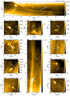 |
Fig. 1. Context for the Solar Orbiter HRIEUV observations of the eleven cases showing thin coronal jets (gray arrows) associated with CBPs that are analyzed in this paper. The intensity of the images is given in DN and times are in UT. The details of each observation are provided in Table 1. Individual movies for each of the cases are available online. |
Properties of the CBPs and their associated thin coronal jets.
3.1. Case 01: 2023-04-07.
This event occurred within a coronal hole and shows two types of behavior: a gentle phase followed by an enhanced phase (see Fig. 1 and associated animation). The gentle phase initially exhibited faint brightenings at 04:23:00 UT around coordinates X = 3.8 and Y = 5.5 Mm. By 04:33:00 UT, a small inverted Y-shaped structure became apparent, centered at X = 5.5 and Y = 5.6 Mm. The activity in this region increased, revealing a distinct fan-spine structure at 04:43:51 UT, with several coronal jets propagating along the outer spine. At 05:19:30 UT, the longest narrow jet of this phase was observed emerging from the fan base, extending across the entire HRIEUV field of view (FOV). In Fig. 2, we analyze the properties of this jet. Panel a shows the context, indicating the location of the thin jet with an arrow. We also superimpose a bent slit of width W and length L to characterize the jet, following the approach taken in Joshi et al. (2017) and Petrova et al. (2024). Panel b presents the corresponding space-time plot, obtained by extracting the maximum intensity along W from the region defined in panel a. There, we observe that the jet reaches a projected length of Ljet = 22.1 Mm and a velocity of 102 km s−1. In addition, several other jets are visible before and after this one, exhibiting comparable velocities but apparent lengths below 8 Mm. Panel c displays the intensity profile along W at L = 7.5 Mm. The jet width is determined from the full width at half maximum (FWHM) of the intensity profile. The baseline for the FWHM is set as the average intensity at the endpoints of the perpendicular cut. The resulting width shows that this long jet is as thin as wjet = 253 km. Given that in case 01, the pixel size is 108 km (Table 1), this example demonstrates HRIEUV’s ability to resolve very narrow coronal jets. In fact, this event is not detectable in AIA (see Appendix A).
The enhanced phase occurs later, between 05:42:00 UT and 05:44:30 UT, and leads to the brightest jet observed in case 01. Panel d of Fig. 2 illustrates this jet, which exhibits a much broader base compared to those seen during the gentle phase, and reaches a projected length of Ljet = 21.7 Mm. The speed of the jet is approximately 137 km s−1 as shown in panel e. By measuring its FWHM at L = 7.5 Mm, we find that the jet width is wjet = 310 km. The transition from the gentle to the enhanced phase possibly reflects different reconnection regimes. As discussed later in Sect. 4.2, this enhanced phase may result from plasmoid-mediated magnetic reconnection.
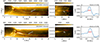 |
Fig. 2. Analysis of case 01 during the gentle reconnection phase at 05:19:30 UT (top row) and the enhanced phase at 05:44:00 UT (bottom row). Panels a and d show the CBP and the associated thin coronal jets (gray arrows). Panels b and e display space–time maps obtained by taking the maximum intensity along the width, W, of the bent red slit of length L shown in panels a and d, respectively. Panels c and f illustrate the widths of the narrow jets, calculated using the FWHM at L = 7.5 Mm, as indicated by the blue dotted lines in panels a and d, respectively. |
3.2. Case 02: 2023-04-05.
The observation for case 02 was conducted in two sequences (see Table 1). According to HMI data (Fig. B.2), this CBP exhibits a canonical photospheric magnetic field configuration typical of CBPs: a parasitic polarity, negative in this case, surrounded by an oppositely signed magnetic field. Figure 1 shows the CBP of interest, centered at X = 8 and Y = 12.5 Mm, with a diameter of approximately 4 Mm, placing it at the lower end of the size distribution (Madjarska 2019). The CBP brightness and associated jet activity fluctuate over time across both sequences. The longest coronal jet emanating from the CBP is clearly visible at 04:01:25 UT (the time of the image), with a length of Ljet = 9.1 Mm and a width of wjet = 326 km (see Appendix B and Fig. B.3 for the calculation details).
3.3. Case 03: 2023-04-04.
Similarly to case 02, this event is also observed in two sequences. If inspected using HMI (Fig. B.2), this area seems to correspond to an emerging region where the parasitic polarity is positive. In Fig. 1, a well-defined and broad CBP, with an elliptical shape and a major axis diameter of approximately 20 Mm, is observed just above the edge of the HRIEUV FOV. A thin jet is visible from the very first frame of observations, departing from the CBP at X = 20 Mm and Y = 14 Mm. It exhibits a recurring pattern throughout the entire duration of the first sequence. At the time shown in Fig. 1, the jet has a length of Ljet = 15.4 Mm and a width of wjet = 629 km (see also Appendix B). A series of broader jets are also observed adjacent to the thin outer spine, appearing at 04:47:58 UT, followed by subsequent occurrences at 05:05:18, 06:01:58, and 06:09:23 UT. During the second sequence, the long and thin jet from the CBP becomes visible at 06:33:29 UT, followed by the emergence of broad jets originating from the CBP footpoints adjacent to it.
3.4. Case 04: 2022-03-22.
The first EUV signatures become visible at 14:06:10 UT, quickly developing the characteristic loops with enhanced EUV emissivity typical of a CBP. The CBP seems to be nearby a region exhibiting a clear negative parasitic polarity (see Fig. B.2). The maximum projected diameter of the CBP is around 6 Mm (Fig. 1), which falls within the lower range of CBP sizes (Madjarska 2019). A thin coronal jet with width wjet = 374 km is ejected from the top of the CBP, reaching its longest extension: Ljet = 4.1 Mm at 14:23:10 UT. Subsequently, the CBP dissipates at 14:25:40 UT, resulting in a CBP lifetime of around 19 minutes.
3.5. Case 05: 2022-03-18.
This large CBP remains visible throughout the entire time series, with an elliptical shape and a major axis diameter of approximately 20 Mm. The jet of interest starts appearing at the corner of the CBP around 10:36:35 UT, specifically, at X = 24 Mm, Y = 12 Mm, following a series of complex dynamic events. We could tentatively relate this event to a dark, elongated structure that might correspond to a small-scale filament, consistent with those reported, for instance, by Panesar et al. (2018) and Kumar et al. (2019a), or to a rising chromospheric fibril, as seen in the observations by Madjarska et al. (2021) and in the 3D simulations of Nóbrega-Siverio et al. (2023). However, in the absence of coordinated chromospheric observations, we refrain from drawing firm conclusions. The current sheet associated with this jet is also clearly discernible, with a length of LCS = 2.8 Mm, approximately. At the time shown in Fig. 1, the jet shows a nice contrast against the background and has a length of Ljet = 5.8 Mm and a width of wjet = 481 km (see Appendix B). Later, at 11:04:55 UT, a dark, absorbing structure interacts with the current sheet, triggering a more eruptive event with a broader jet.
3.6. Case 06: 2022-03-17.
The 30-minute sequence reveals a rapidly evolving CBP with a maximum projected diameter of approximately 6 Mm, also placing this event at the lower end of the CBP size distribution (Madjarska 2019). HMI data indicate that this case corresponds to a CBP with a negative parasitic polarity in the photosphere (Fig. B.2). The largest thin coronal jet associated with this CBP occurs at 03:42:36 UT (Fig. 1) with a length of Ljet = 21.8 Mm and a width of wjet = 344 km (see Appendix B), and has a counterpart in AIA 171 Å (see Fig. B.1).
3.7. Case 07: 2022-10-26.
Case 07 corresponds to a small and short-lived CBP. The first signatures of the CBP appear around 19:14:20 UT. HMI data suggest that an emerging dipole, with a positive parasitic polarity, may have occurred at this location. By 19:17:45 UT, a distinct bidirectional ejection emerges from the CBP, featuring two spines extending to the north and south. The bidirectional jets reach their maximum extent at 19:20:30 UT, with lengths around Ljet = 5.5 Mm and widths of wjet = 382 km (see Appendix B). In AIA 171 Å, we might infer their presence based on the HRIEUV observations (Fig. B.1). The bidirectional jet configuration resembles that studied in AIA by Ruan et al. (2019) and in numerical experiments with horizontal coronal magnetic field (e.g., Yokoyama & Shibata 1996; Archontis et al. 2005; Syntelis et al. 2019; Færder et al. 2023). In fact, just before the jets, we might be able to identify a dark structure ejected above the CBP, which could represent part of the emerging dome being expelled as a plasmoid or surge, as shown in simulations (see Archontis et al. 2006; Nishizuka et al. 2008; Jiang et al. 2012; Moreno-Insertis & Galsgaard 2013; Nóbrega-Siverio et al. 2016, 2018, among others). However, chromospheric observations are required for a clear conclusion. Afterward, the CBP gradually fades and disappears by 19:22:05 UT, resulting in a total lifetime of approximately 8 minutes.
3.8. Case 08: 2022-10-29.
This CBP, akin to cases 02 and 03, was observed in two sequences, although there is a 2.5-hour gap between them and the HRIEUV exposure time was adjusted for the second one (see Table 1). The CBP, with a projected diameter of approximately 15 Mm, is already visible in the first frame of the first sequence and remains discernible until the end of the second sequence, resulting in a lifetime of more than 3.5 hours. HMI data reveal that the CBP of interest is rooted in a negative parasitic polarity, surrounded by a region of positive magnetic polarity. The animation shows recurrent coronal jets that are faint and narrow. For instance, the jet shown in Fig. 1 reaches a length of Ljet = 19.5 Mm and a width of wjet = 411 km (see also Appendix B). All these jets originate from a very thin and highly dynamic current sheet located at the top of the CBP, centered at X = 26 Mm and Y = 17 Mm. This current sheet is particularly interesting, as it shows clear signatures of non-stationary magnetic reconnection, including the presence of a well-defined plasmoid. A detailed analysis of the plasmoid and its dynamic behavior is presented in Sect. 4.1.
3.9. Case 09: 2023-10-24.
This event was observed for nearly 2 hours. At the beginning of the HRIEUV sequence, the CBP exhibits an ellipse-like shape with a major axis of approximately 25 Mm. As in other cases, HMI shows that the CBP is rooted in a negative parasitic polarity. The CBP is highly dynamic and displays a microflare-like structure around 12:24:00 UT, accompanied by a collimated flow. Similar to case 05, this event may be related to enhanced chromospheric activity, possibly involving either a small-scale filament or a rising fibril; nonetheless, coordinated chromospheric observations are required to disentangle the scenario. The thin jet observed at 12:28:20 UT in Fig. 1 reaches a length of Ljet = 16.1 Mm and a width of wjet = 706 km, and disappears shortly afterward (see Appendix B). In AIA 171 Å, it is also possible to discern it (Fig. B.1). An analogous jetting pattern is seen at 12:32:40, 12:58:30, 13:15:50, and 13:44:50 UT. By the end of the observational sequence, the CBP had become narrower compared to its initial state.
3.10. Case 10: 2023-10-29.
In this case, the HRIEUV FOV encompasses multiple adjacent CBPs, the largest of which is located at approximately X = 23 and Y = 13 Mm. HMI magnetograms reveal three negative polarity patches embedded within a dominant positive field, which may account for the presence of multiple CBPs in the region. The largest CBP has a very distinguishable fan base with a thin jet extending from its top at 07:15:32 UT. In line with other events, the jetting activity is intermittent. At 07:25:02 UT (see Fig. 1), the CBP displayed the clearest narrow jet from its base, with a length of Ljet = 7.5 Mm and a width of wjet = 637 km, which disappeared by the end of the HRIEUV observation at 07:29:52 UT (see also Appendix B).
3.11. Case 11: 2021-09-14.
Among the events studied here, this CBP has been captured from the greatest distance and with the shortest exposure time (see Table 1), which explains why the image quality appears slightly lower than in the other cases. The CBP is present throughout the entire time series with a diameter of approximately 6 Mm and it is anchored in a region with a positive parasitic polarity, as seen in HMI. A very thin jet appears at 07:05:02 UT and remains discernible for almost 6 minutes. At the time shown in Fig. 1, the jet has an extension of Ljet = 6.7 Mm and a width of wjet = 591 km. Due to the short duration of this observation, the reappearance of the outer spine, as seen in most other cases, could not be captured.
4. Signatures of plasmoid-mediated reconnection: Comparison with numerical models
4.1. Direct plasmoid detection
We detected a clear case of a plasmoid being formed and ejected within the current sheet of the CBP in case 08. To illustrate this, we refer to Fig. 3 and the accompanying animation. Panel a shows the CBP and the associated current sheet, highlighted by a red rectangle of length, L, and width, W, at the time when the plasmoid is most clearly visible (19:10:50 UT). Panel b presents a zoom into the region around the current sheet, corresponding to the blue rectangle in panel a. The cyan arrow indicates a bright, blob-like feature, which we interpret as a plasmoid. Its size is approximately two pixels in each direction, corresponding to about 332 km. To analyze its motion, we measured the maximum intensity along the W direction within the slanted red rectangle. The results are shown as a space–time plot in panel c. The plasmoid displays a projected velocity of approximately 40 km s−1. Panel d contains intensity profiles along the current sheet at different times, tracking the temporal evolution of the detected plasmoid. From this panel and the accompanying animation, weestimated the plasmoid’s lifetime to be around 20 seconds.
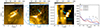 |
Fig. 3. Plasmoid signatures in case 08. Panel a: Context view showing the CBP and the current sheet within a rectangle of length, L, and width, W. Panel b: Zoomed-in view of the blue rectangle shown in panel a, highlighting the illustrative plasmoid with a cyan arrow. Panel c: Space–time plot of the current sheet, obtained by taking the maximum intensity along the W direction. The cyan dashed line indicates the trajectory of the plasmoid. Panel d: Intensity profiles along the current sheet at different times, illustrating the evolution of the plasmoid indicated in panel c. An animation of this figure is available on zenodo and online, showing the evolution of the plasmoid between 19:10:35 UT and 19:11:10 UT. |
To support this finding, we compared the Solar Orbiter results with those from the CBP numerical experiment (see Sect. 2.2). Figure 4 and the associated animation show the synthetic HRIEUV emissivity derived from the simulation, using the same panel layout as in Fig. 3. The top row displays the simulation at its native resolution (≈16 km), while the bottom row shows the same results after degrading the image to the best-case scenario achieved by HRIEUV in this study (pixel size of 108 km). The first column provides context at a time when a clear plasmoid is present (t = 29.97 min), showing enhanced synthetic emissivity in the CBP loops (located between x = 19 and 30 Mm) and the jet spine extending upward from z = 9 Mm at x = 30.4 Mm. In the second column, a bright plasmoid can be clearly distinguished within the current sheet. At the native resolution (panel b), the plasmoid has an estimated length of 300 km and a width of 200 km, approximately, which is large enough to be resolved by HRIEUV. Panel f confirms this: although the plasmoid appears more subtle after resolution degradation, it remains detectable as a cluster of pixels with enhanced emissivity, in close resemblance to the observational case. The third column shows the plasmoid’s motion through space–time maps. Its signature resembles the observational one shown in Fig. 3, although it travels faster in the simulation, with a velocity of 148 km s−1 (see Sect. 5 for a discussion on the differences in plasmoid velocities). Finally, the fourth column displays the intensity profiles along the current sheet at different times, capturing the temporal evolution of the plasmoid. Even after degrading the resolution, the plasmoid remains detectable through triangular-shaped intensity peaks moving along the current sheet, consistent with the observational findings.
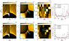 |
Fig. 4. Same as Figure 3, but for the plasmoid signatures in the 2D CBP simulation by Nóbrega-Siverio & Moreno-Insertis (2022). Top row shows the HRIEUV synthetic emissivity at the original resolution of the numerical experiment (≈16 km). Bottom row shows the results after degrading the resolution to match the best case achievable by HRIEUV in our study (pixel size of 108 km). An animation of this figure is available on zenodo and online, showcasing the plasmoid evolution between t = 29.9 and t = 30.0 min. |
4.2. Indirect signatures of plasmoids
In case 01, we find imprints in the outflow region that could be a consequence of plasmoid-mediated reconnection. Since no plasmoids are directly detected in HRIEUV, we refer to these as potential indirect signatures. This is illustrated in Fig. 5 and the associated animation. In panel a, the brightest jet is shown to provide context, with arrows indicating a double adjacent boomerang-like discontinuous pattern that appears slightly brighter than its surroundings. To further inspect this feature, in panel b we present a space-time map of the intensity along the slit of length, L, indicated in panel a. The structure appears as two nearly vertical bands, with an apparent velocity of only a few kilometers per second. In panel c, we show the intensity profile along the slit at time 05:44:00 UT. The arrows indicate two small humps, standing slightly enhanced compared to the surrounding regions. We conjecture that this feature is a consequence of plasmoids being ejected and colliding with the pre-existing magnetic field, potentially explaining the transition from a gentle reconnection phase to an enhanced phase associated with the brightest jet of case 01.
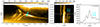 |
Fig. 5. Indirect signatures of plasmoid-mediated reconnection in case 01. Panel a: Context view illustrating the CBP and the associated ejections. The arrows mark the signatures that are interpreted as consequences of plasmoid-mediated magnetic reconnection. Panel b: Space–time map obtained by sampling the intensity along the slit of length L shown in panel a. Panel c: Intensity profiles along the slit at 05:44:00 UT. An animation of this figure is available online, showing the time evolution between 05:43:48 UT and 05:44:12 UT. |
To support this hypothesis, we turn to the simulations, from an instant approximately 22 min later than that shown in Fig. 4. Figure 6 shows maps over a 10-second time window of the temperature (column a); nenH, the product of the electron and hydrogen number densities, which is a key factor in computing the emissivity under optically thin conditions (column b); and the synthetic HRIEUV emissivity at the simulation’s native resolution (column c). In all maps, the axes have been transposed so that height appears along the horizontal axis, mimicking the morphology of the jet observed in case 01. The top row maps highlight the location of the post-reconnection loops that give rise to the CBP, the jet spine, and the current sheet (CS). A plasmoid, labeled as 1, is identified within the current sheet in both the temperature and nenH maps between t = 52.43 min and t = 52.47 min. However due to its high temperature (≈3 MK), it is not directly visible in HRIEUV, whose response function peaks at ≈0.9 MK (see, e.g., Chen et al. 2021; Dolliou et al. 2023). At t = 52.50 min, plasmoid 1 collides with the pre-existing field, generating a shock and losing its identity as a closed magnetic island via reconnection. Consequently, the density originally confined within the plasmoid is redistributed along the newly reconnected field line. Following the subsequent evolution in the outflow region, a boomerang-like structure develops, exhibiting slightly enhanced density and HRIEUV emissivity relative to its surroundings, most clearly seen at t = 52.60 min. In this 10-second time window, a second plasmoid, labeled as 2, is also detected within the current sheet at t = 52.50 min in the nenH map propagating in the same direction as plasmoid 1. Its increasing density, combined with a lower temperature than that of plasmoid 1, makes it visible two seconds later in the HRIEUV map (t = 52.52 min). Then, it collides with the pre-existing field, generating another boomerang-like structure with enhanced emissivity. Due to the intermittent nature of plasmoid-mediated reconnection, multiple boomerang-like patterns appear over time in the outflow region of the simulation.
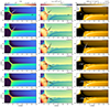 |
Fig. 6. Indirect signatures of plasmoid-mediated reconnection in the outflow region from the 2D CBP simulation by Nóbrega-Siverio & Moreno-Insertis (2022) between t = 52.43 and t = 52.60 min. We have transposed the axes so that height appears on the horizontal axis to ease the comparison with the observations. Column (a): Temperature maps. Column (b): nenH, the product of the electron and hydrogen number densities. Column (c): HRIEUV synthetic emissivity at the original resolution of the experiment (≈16 km). The three panels of the top row include the locations of the CBP, the current sheet (CS), and the jet. The arrows 1 and 2 follow the formation and ejection of two different plasmoids along with their signatures in the outflow region. |
With respect to the consistency between this scenario and the observations. The simulations show that current sheets can host plasmoids that are challenging to detect with Solar Orbiter HRIEUV. Plasmoid 1 is too hot to fall within the instrument’s response range. Plasmoid 2, in contrast, evolves so rapidly that it appears in HRIEUV emissivity only in a single snapshot of the numerical experiment, despite the simulation having a 2-second cadence: a cadence that is already shorter than that of any of the HRIEUV observations presented in this paper. Nevertheless, the impact of these plasmoids can still leave observable imprints after they leave the current sheet. In particular, the simulations reveal the formation of boomerang-like structures in the outflow region that closely resemble those seen in case 01. To further illustrate the similarity with observations, we refer to Fig. 7 and the associated animation. Panel a shows the emissivity map from the simulation at t = 52.60 min, degraded to match the best spatial resolution achievable by Solar Orbiter HRIEUV. Even after degradation, the boomerang-like pattern generated in the outflow region by multiple plasmoids remains discernible (see arrows). In panel b, the space–time map, calculated along the slit of length, L, shown in panel a, illustrates how the discontinuous pattern propagates at a velocity of approximately 23 km s−1. In the intensity profile at t = 52.60 min (panel c), we identify the corresponding small humps, slightly enhanced with respect to the surrounding regions, closely resembling those seen in the observations. This supports the interpretation that indirect signatures of plasmoid-mediated reconnection in the outflow region could indeed be captured by HRIEUV.
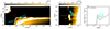 |
Fig. 7. Indirect signatures of plasmoid-mediated reconnection in the outflow region from the 2D CBP simulation by Nóbrega-Siverio & Moreno-Insertis (2022) after degrading the resolution to match the best case achievable by HRIEUV in our study (pixel size of 108 km). Panel a: HRIEUV synthetic emissivity. We have transposed the axes so that height appears on the horizontal axis. Panel b: Space–time map obtained by sampling the intensity along the slit of length L shown in panel a. Panel c: Intensity profiles along the slit at t = 52.60 min. In all the panels, the arrows mark some of the features that are interpreted as consequences of plasmoids previously ejected during the reconnection process. An animation of this figure is available online, including temperature and nenH maps, showcasing the appearance of indirect plasmoid-mediated signatures between t = 52.40 and t = 52.80 min. |
5. Discussion and conclusions
In this work, we used high-resolution Solar Orbiter HRIEUV observations to study eleven datasets that show narrow coronal jets associated with CBPs. In parallel, we analyzed observational signatures indicative of plasmoid-mediated reconnection and interpreted them in light of the radiative-MHD numerical simulations published by Nóbrega-Siverio & Moreno-Insertis (2022). Importantly, these features have been detected without applying any image enhancement techniques such as multiscale Gaussian normalization (MGN; Morgan & Druckmüller 2014) or wavelet-optimized whitening (WOW; Auchère et al. 2023). This underscores the state-of-the-art capability of HRIEUV for capturing fine-scale jets and key dynamic signatures from a vantage point close to the Sun. In the following, we discuss the broader implications of our findings and present the main conclusions.
5.1. Thin coronal jets from CBPs
In Sect. 3, we identified coronal jets originating from CBPs with widths ranging from 253 km to 706 km: scales that could not be resolved with previous EUV imaging instruments, where jet widths were typically reported to be above 2 Mm (see, e.g., Shimojo et al. 1996; Savcheva et al. 2007; Raouafi et al. 2016; Joshi et al. 2017; Shen 2021; Panesar et al. 2023). Remarkably, these jets extend up to projected lengths of 22 Mm (cases 01 and 06), while maintaining their narrow structure. This demonstrates that jet outflows can propagate over long distances along narrow structures and potentially contribute to the solar wind. The most comparable event observed in HRIEUV to our longest thin CBP jet (case 01) is reported by Petrova et al. (2024), where the authors detected torsional motions propagating along the outer spine. Interestingly, these narrow jets can originate from quite compact CBPs. In fact, seven out of our eleven CBPs have projected diameters ranging from 6 Mm down to 3 Mm (see Table 2), placing them at the lower end of the CBP size distribution (Madjarska 2019). Similar compact bright points associated with narrow jets have also been reported using AIA, near the instrument’s resolution limit (Kumar et al. 2019a, 2022).
To place our results in the context of recent HRIEUV findings, we compare them with the recently reported picoflare jets by Chitta et al. (2023, 2025). The picoflare jets are inverted Y-shaped structures that extend only a few hundred kilometers, appearing 10% to 30% brighter than the surrounding coronal hole, with lifetimes ranging from 20 to 100 seconds. Picoflare jets have widths of a few hundred kilometers, comparable to our CBP-associated jets, although the latter are larger in extent and exhibit brightness enhancements between 30% and 85% relative to their surroundings (see Appendix B.3). Both types of jets, namely, picoflare jets and the longer CBP-associated thin jets presented here, underscore the capabilities provided by HRIEUV for studying fine-scale coronal dynamics.
In the HRIEUV time windows analyzed for the eleven cases, we did not observe large blowout jets and associated filament eruptions, in line with the results of some numerical models (e.g., Archontis & Hood 2013; Moreno-Insertis & Galsgaard 2013; Fang et al. 2014; Pariat et al. 2015; Lee et al. 2015; Wyper et al. 2017, 2018a,b; Joshi et al. 2024; Zhuleku et al. 2025; Patsourakos & Archontis 2025, among others). Only two of the cases may be tentatively related to some enhanced chromospheric activity in the form of small-scale filament or chromospheric fibril; nonetheless, since no chromospheric observations are available for these events, a conclusive interpretation cannot be established. Thus, the majority of our observed thin coronal jets seem to be related to the more “gentle” phases of CBP evolution. These stages are characterized by narrow jets of the kind of straight jets modeled by, for instance, Pariat et al. (2010, 2015), which can be produced through an ad-hoc photospheric driving and are not impulsively generated, unlike helical or blowout jets. More recent radiative-MHD models building upon this framework, such as Nóbrega-Siverio & Moreno-Insertis (2022) in 2D and Nóbrega-Siverio et al. (2023) in 3D, have demonstrated that stochastic granular motions are sufficient to stress the CBP’s fan-spine configuration and trigger sustained reconnection at the coronal null point. This reconnection naturally results in persistent jetting activity in the form of thin, recurrent jets.
The keys to detecting narrow coronal jets associated with CBPs are described in the following. High spatial resolution from HRIEUV appears to be essential to resolve the outer spine of the jets, as demonstrated by the comparison presented in Appendix B.1, where some of the jets observed with HRIEUV are barely discernible or completely absent in AIA 171 Å. This is a particularly exciting discovery for the coronal jet community. For instance, using AIA, Kumar et al. (2019a) explicitly noted that CBPs do not produce coronal jets immediately after emergence, reporting delays ranging from approximately two hours for small CBPs to five days for the most significant cases in their sample (see also the review by Madjarska 2019). Muglach (2021) warned that the lack of a jet in AIA during flux emergence should be considered with caution, based on the findings from Young (2015) showing that “there can be coronal hole jets without visible signatures in AIA images”. Thanks to the enhanced spatial resolution of HRIEUV, we may now detect earlier or fainter phases of jet activity related to CBPs.
Alongside spatial resolution, the density contrast between the jet and the surrounding atmosphere appears to be the other decisive factor in this regard. Indeed, CBPs can produce collimated high-speed hot plasma outflows that do not exhibit significant EUV emission due to a relatively low density contrast with their surroundings, as demonstrated in the synthetic observables from the 3D CBP numerical experiment of Nóbrega-Siverio et al. (2023). In fact, there is observational evidence of CBP jets being detected in EUV spectroscopic data from Hinode/EIS, while lacking any corresponding signal in AIA imaging (Young 2015), as well as studies aiming to understand the faintness of solar coronal jets from CBPs located in coronal holes (Harden et al. 2021). This highlights the need not only for high-resolution imaging, but also spectroscopic diagnostics to fully capture the diversity and subtlety of jet activity associated with CBPs. Upcoming missions such as the Multi-slit Solar Explorer (MUSE; Cheung et al. 2022; De Pontieu et al. 2022) and Solar-C/EUVST (Shimizu et al. 2020) are expected to significantly advance this goal by delivering coordinated multiwavelength observations with unprecedented spatial and temporal coverage.
Beyond the challenges involved in making detections, an important open question is whether the jets emerging from CBPs can contribute to the solar wind and its variability. Current observational efforts have combined Parker Solar Probe (PSP; Fox et al. 2016) and AIA data to assess whether jets from CBPs can be precursors of magnetic switchbacks (e.g., Kumar et al. 2023; Hou et al. 2024; Bizien et al. 2025). At the same time, numerical models suggest that interchange reconnection in the low corona, particularly in fan-spine magnetic topologies akin to those of CBPs, have the capacity to produce jets and Alfvénic perturbations capable of propagating into the heliosphere (see, e.g., Wyper et al. 2022; Bale et al. 2023; Touresse et al. 2024). Our detection of narrow jets with HRIEUV reveals a richer and more dynamic jetting activity from CBPs than what was previously accessible, suggesting that CBPs might play a more significant role in shaping the solar wind. This opens up exciting prospects for future studies aiming to clarify the connection between jets from CBPs and in situ solar wind structures.
5.2. Signatures of plasmoid-mediated magnetic reconnection
5.2.1. Direct plasmoid detection
In case 08, the CBP exhibits a thin current sheet of approximately 2.6 Mm in length, from which coronal jets originate. Within this current sheet, we identified a clearly resolved plasmoid forming, reaching a length of 332 km, and propagating at an approximate velocity of 40 km s−1 (Sect. 4.1). The estimated lifetime of the plasmoid is around 20 seconds. The simulation by Nóbrega-Siverio & Moreno-Insertis (2022) shows that the null point of a fan-spine magnetic topology can be self-consistently stressed by perturbations driven by granular motions. This leads to the formation of a current sheet with a length comparable to that inferred from the observations, within which a plasmoid develops and reaches a size similar to the observed one. When the synthetic emission is degraded to HRIEUV resolution, the resulting imprints closely match those observed, despite the simulated plasmoid exhibiting a higher velocity of 148 km s−1. This similarity is striking, considering that this numerical experiment is not intended as a direct reproduction of the observed event; rather, it is meant to serve as a proof of concept for the observable signatures of plasmoid-mediated reconnection. The difference in velocity may arise from projection effects; a higher reconnection rate in the simulation, since plasmoid speeds scale with the Alfvén speed (e.g., Nishida et al. 2009; Nishizuka et al. 2015); different plasma beta (Peter et al. 2019); among others. Notably, our observational result also aligns with the recent simulations by Færder et al. (2024b), who reported plasmoids with sizes between 200−500 km, lifetimes of 10−20 s, and velocities up to 50 km s−1 in coronal fan-spine topologies, concluding that such features should be observable with HRIEUV.
Plasmoids have a long and rich history in physics (Furth et al. 1963) and their theoretical understanding has significantly advanced, with key developments in the regime of fast reconnection driven by plasmoid instabilities (e.g., Loureiro et al. 2007, 2012; Bhattacharjee et al. 2009; Uzdensky et al. 2010, among many others). To our knowledge, the direct evidence presented here constitutes the smallest plasmoid forming and propagating within a current sheet ever reported in coronal EUV observations. Thus, our findings contribute to the large body of observational and numerical efforts regarding plasmoids developed over the past decade. These include observational plasmoid diagnostics supported by simulations in various eruptive contexts (e.g., Innes et al. 2015; Rouppe van der Voort et al. 2017; Kumar et al. 2019b; Yan et al. 2022; Cheng et al. 2024) and advanced MHD models capturing plasmoid dynamics (e.g., Ni et al. 2015, 2021; Wyper et al. 2016; Nóbrega-Siverio et al. 2017; Hansteen et al. 2019; Li et al. 2023; Sen & Moreno-Insertis 2025), as well as ultra-high-resolution Hα observations revealing the finest-scale signatures of magnetic reconnection (e.g., Rouppe van der Voort et al. 2023; Kumar et al. 2024). The most similar plasmoid scenarios to our observations, combining HRIEUV and AIA observations, are described by Mandal et al. (2022), who reported blobs with sizes between 1−2 Mm within the current sheet of a coronal jet observed at the limb. We also have the study from Cheng et al. (2023), who identified blob-like features with lifetimes ranging from 5 to 105 s. The latter referred to them as outflow blobs, which propagate along the fan surface of a CBP and the jet’s outer spine. These types of blobs (plasmoids) have also been reported using AIA alone in similar jet contexts (see, e.g., Zhang & Ji 2014; Zhang & Ni 2019; Kumar et al. 2019b; Joshi et al. 2020; Mulay et al. 2023).
The plasmoid analyzed in this paper represents the clearest observational case identified in our dataset. However, the animation associated with case 08 (Fig. 1) reveals the intermittent jetting activity and dynamic behavior of the current sheet, strongly suggesting that multiple plasmoids may be forming and evolving throughout the event, even if only one is clearly resolved. It is important to emphasize that detecting and tracking such plasmoids requires a delicate balance between high spatial resolution, high temporal cadence, and sufficient exposure time. In case 08, the cadence is Δt = 5 s (see Table 1), which allows us to clearly resolve the small-scale plasmoid in four consecutive frames. The exposure time is texp = 1.65 s, which provides a sufficiently long signal, while still being short enough not to compromise the cadence. By contrast, when the exposure time drops to texp = 0.70 s, as in case 11, the jet and associated features in the coronal hole become significantly noisier and harder to analyze. Thus, based on the instrumental configurations of cases 01 and 08, along with previous similar reports (Mandal et al. 2022; Cheng et al. 2023), we tentatively suggest that an exposure time in the range texp ∈ [1.65, 2.80] s and a cadence of Δt ∈ [3, 5] s could provide an optimal balance for studying plasmoid-related signatures in comparable scenarios using HRIEUV.
5.2.2. Indirect signatures of plasmoids
Plasmoids cannot always be directly detected in observations due to their scale or rapid evolution, or because the associated temperature falls outside the bandpass’s response function. Unlike AIA, HRIEUV does not observe multiple wavelengths simultaneously at the same resolution, which highlights the need for high-resolution imaging combined with broader temperature diagnostics. Still, using a single bandpass, we could find observational signatures in the outflow region that could suggest the presence of plasmoid-mediated reconnection. This is explored in Sect. 4.2, where we describe our analysis of a repeating, boomerang-like pattern with slightly enhanced intensity in the outflow region near the CBP jet of case 01. To support this conjecture, we made a comparison with the numerical simulations, showing that when plasmoids are expelled from the current sheet, they collide with the ambient magnetic field and undergo secondary reconnection, losing their identity as closed magnetic islands. The plasma originally confined within the plasmoids is redistributed along the newly reconnected field lines. Because plasmoid-mediated reconnection is inherently bursty, this process creates a sequence of localized density enhancements, separated by lower density regions. Given that optically thin emission depends quadratically on the plasma density, this leads to a discontinuous brightness pattern that is consistent with the boomerang-like features observed with HRIEUV.
We cannot completely exclude the possibility that the observed pattern arises from an intermittent reconnection driver rather than from plasmoid ejections. However, two key elements lead us to consider plasmoid-mediated reconnection as a plausible scenario in this case. First, the observed features bear striking similarities to the synthetic HRIEUV emission derived from the Bifrost simulation, where the presence of plasmoids in density is unambiguous. Second, the observed jetting activity of the CBP of case 01 transitions from a gentle phase to a more explosive one, which could indicate a change in the reconnection regime, from a smooth to a plasmoid-mediated regime, consistent with theoretical expectations for current sheet evolution in high-Lundquist number plasmas. Moreover, boomerang-like patterns in the outflow region appear to be a generic signature rather than a peculiarity of our simulation. Indeed, similar signatures can be seen in synthetic EUV emission from other numerical models with null-point topologies and plasmoid-mediated reconnection, such as those depicted in Fig. 6 of Gannouni et al. (2023) and Fig. 5 of Færder et al. (2024b), although they have not been discussed in depth by the respective authors. Therefore, these indirect signatures provide valuable insights into the presence of plasmoid-mediated reconnection, complementing other forms of indirect evidence, such as wave-like perturbations along the jet spine (e.g., Gannouni et al. 2023; Hou et al. 2025) or quasi-periodic pulsations (QPPs) associated with reconnection dynamics (e.g., McLaughlin et al. 2018; Kumar et al. 2025).
Data availability
Movies associated with Figs. 3 and 4 are available at https://www.aanda.org All the movies are available at https://zenodo.org/records/16903189
Acknowledgments
We thank the referee for their constructive feedback to improve the presentation and contextualization of the manuscript. This research has been supported by the European Research Council through the Synergy Grant number 810218 (“The Whole Sun”, ERC-2018-SyG) and by the Research Council of Norway (RCN) through its Centres of Excellence scheme, project number 262622. D.N.S. and R.J. gratefully acknowledge the Solar Orbiter/EUI Guest Investigator program, and thank Marilena Mierla for her kind support during their two research stays at the Royal Observatory of Belgium. D.N.S. also acknowledges the support by Aletheia Solaris. D.L. was supported by a Senior Research Project (G088021N) of the FWO Vlaanderen and the Belgian Federal Science Policy Office through the contract B2/223/P1/CLOSE-UP. Solar Orbiter is a space mission of international collaboration between ESA and NASA, operated by ESA. The EUI instrument was built by CSL, IAS, MPS, MSSL/UCL, PMOD/WRC, ROB, LCF/IO with funding from the Belgian Federal Science Policy Office (BELSPO/PRODEX PEA 4000112292 and 4000134088); the Centre National d’Etudes Spatiales (CNES); the UK Space Agency (UKSA); the Bundesministerium für Wirtschaft und Energie (BMWi) through the Deutsches Zentrum für Luft- und Raumfahrt (DLR); and the Swiss Space Office (SSO). The authors also acknowledge the computer resources at the MareNostrum supercomputing installation and the technical support provided by the Barcelona Supercomputing Center (BSC, RES-AECT-2021-1-0023, RES-AECT-2022-2-0002), as well as the resources provided by Sigma2 – the National Infrastructure for High Performance Computing and Data Storage in Norway.
References
- Archontis, V., & Hood, A. W. 2013, ApJ, 769, L21 [Google Scholar]
- Archontis, V., Moreno-Insertis, F., Galsgaard, K., & Hood, A. W. 2005, ApJ, 635, 1299 [NASA ADS] [CrossRef] [Google Scholar]
- Archontis, V., Galsgaard, K., Moreno-Insertis, F., & Hood, A. W. 2006, ApJ, 645, L161 [NASA ADS] [CrossRef] [Google Scholar]
- Auchère, F., Soubrié, E., Pelouze, G., & Buchlin, É. 2023, A&A, 670, A66 [NASA ADS] [CrossRef] [EDP Sciences] [Google Scholar]
- Bale, S. D., Horbury, T. S., Velli, M., et al. 2021, ApJ, 923, 174 [NASA ADS] [CrossRef] [Google Scholar]
- Bale, S. D., Drake, J. F., McManus, M. D., et al. 2023, Nature, 618, 252 [NASA ADS] [CrossRef] [Google Scholar]
- Berghmans, D., Auchère, F., Long, D. M., et al. 2021, A&A, 656, L4 [NASA ADS] [CrossRef] [EDP Sciences] [Google Scholar]
- Bhatnagar, A., Prasad, A., Nóbrega-Siverio, D., van der Voort, L. R., & Joshi, J. 2025, A&A, 698, A174 [NASA ADS] [CrossRef] [EDP Sciences] [Google Scholar]
- Bhattacharjee, A., Huang, Y.-M., Yang, H., & Rogers, B. 2009, Phys. Plasmas, 16, 112102 [Google Scholar]
- Bizien, N., Froment, C., Madjarska, M. S., Dudok de Wit, T., & Velli, M. 2025, A&A, 694, A181 [NASA ADS] [CrossRef] [EDP Sciences] [Google Scholar]
- Bose, S., Nóbrega-Siverio, D., De Pontieu, B., & Rouppe van der Voort, L. 2023, ApJ, 944, 171 [NASA ADS] [CrossRef] [Google Scholar]
- Chen, Y., Przybylski, D., Peter, H., et al. 2021, A&A, 656, L7 [NASA ADS] [CrossRef] [EDP Sciences] [Google Scholar]
- Chen, Y., Mandal, S., Peter, H., & Chitta, L. P. 2024, A&A, 692, A119 [NASA ADS] [CrossRef] [EDP Sciences] [Google Scholar]
- Cheng, X., Priest, E. R., Li, H. T., et al. 2023, Nat. Commun., 14, 2107 [Google Scholar]
- Cheng, G., Ni, L., Tang, Z., et al. 2024, ApJ, 966, L29 [NASA ADS] [CrossRef] [Google Scholar]
- Cheung, M. C. M., Martínez-Sykora, J., Testa, P., et al. 2022, ApJ, 926, 53 [NASA ADS] [CrossRef] [Google Scholar]
- Chitta, L. P., Peter, H., Parenti, S., et al. 2022, A&A, 667, A166 [NASA ADS] [CrossRef] [EDP Sciences] [Google Scholar]
- Chitta, L. P., Zhukov, A. N., Berghmans, D., et al. 2023, Science, 381, 867 [NASA ADS] [CrossRef] [Google Scholar]
- Chitta, L. P., Huang, Z., D’Amicis, R., et al. 2025, A&A, 694, A71 [NASA ADS] [CrossRef] [EDP Sciences] [Google Scholar]
- De Pontieu, B., Testa, P., Martínez-Sykora, J., et al. 2022, ApJ, 926, 52 [NASA ADS] [CrossRef] [Google Scholar]
- Dolliou, A., Parenti, S., Auchère, F., et al. 2023, A&A, 671, A64 [NASA ADS] [CrossRef] [EDP Sciences] [Google Scholar]
- Dolliou, A., Parenti, S., & Bocchialini, K. 2024, A&A, 688, A77 [NASA ADS] [CrossRef] [EDP Sciences] [Google Scholar]
- Duan, Y., Chen, H., Hou, Z., Sun, Z., & Shen, Y. 2025, ApJ, 979, 195 [Google Scholar]
- Færder, Ø. H., Nóbrega-Siverio, D., & Carlsson, M. 2023, A&A, 675, A97 [NASA ADS] [CrossRef] [EDP Sciences] [Google Scholar]
- Færder, Ø. H., Nóbrega-Siverio, D., & Carlsson, M. 2024a, A&A, 683, A95 [NASA ADS] [CrossRef] [EDP Sciences] [Google Scholar]
- Færder, Ø. H., Nóbrega-Siverio, D., Carlsson, M., & Martínez-Sykora, J. 2024b, A&A, 687, A171 [NASA ADS] [CrossRef] [EDP Sciences] [Google Scholar]
- Fang, F., Fan, Y., & McIntosh, S. W. 2014, ApJ, 789, L19 [NASA ADS] [CrossRef] [Google Scholar]
- Fargette, N., Lavraud, B., Rouillard, A. P., et al. 2021, ApJ, 919, 96 [NASA ADS] [CrossRef] [Google Scholar]
- Fox, N. J., Velli, M. C., Bale, S. D., et al. 2016, Space Sci. Rev., 204, 7 [Google Scholar]
- Furth, H. P., Killeen, J., & Rosenbluth, M. N. 1963, Phys. Fluids, 6, 459 [Google Scholar]
- Galsgaard, K., Madjarska, M. S., Moreno-Insertis, F., Huang, Z., & Wiegelmann, T. 2017, A&A, 606, A46 [NASA ADS] [CrossRef] [EDP Sciences] [Google Scholar]
- Gannouni, B., Réville, V., & Rouillard, A. P. 2023, ApJ, 958, 110 [NASA ADS] [CrossRef] [Google Scholar]
- Gao, Y., Tian, H., Berghmans, D., et al. 2025, ApJ, 985, L12 [Google Scholar]
- Gudiksen, B. V., Carlsson, M., Hansteen, V. H., et al. 2011, A&A, 531, A154 [NASA ADS] [CrossRef] [EDP Sciences] [Google Scholar]
- Hansteen, V., Ortiz, A., Archontis, V., et al. 2019, A&A, 626, A33 [NASA ADS] [CrossRef] [EDP Sciences] [Google Scholar]
- Harden, A. R., Panesar, N. K., Moore, R. L., Sterling, A. C., & Adams, M. L. 2021, ApJ, 912, 97 [Google Scholar]
- Hong, J., Jiang, Y., Yang, J., et al. 2014, ApJ, 796, 73 [NASA ADS] [CrossRef] [Google Scholar]
- Hou, C., Rouillard, A. P., He, J., et al. 2024, ApJ, 968, L28 [NASA ADS] [CrossRef] [Google Scholar]
- Hou, C., Gannouni, B., Rouillard, A. P., He, J., & Réville, V. 2025, A&A, 697, A67 [NASA ADS] [CrossRef] [EDP Sciences] [Google Scholar]
- Huang, Z., Teriaca, L., Aznar Cuadrado, R., et al. 2023, A&A, 673, A82 [NASA ADS] [CrossRef] [EDP Sciences] [Google Scholar]
- Innes, D. E., Guo, L. J., Huang, Y. M., & Bhattacharjee, A. 2015, ApJ, 813, 86 [Google Scholar]
- Jiang, R. L., Fang, C., & Chen, P. F. 2012, ApJ, 751, 152 [NASA ADS] [CrossRef] [Google Scholar]
- Joshi, R., Schmieder, B., Chandra, R., et al. 2017, Sol. Phys., 292, 152 [NASA ADS] [CrossRef] [Google Scholar]
- Joshi, R., Chandra, R., Schmieder, B., et al. 2020, A&A, 639, A22 [NASA ADS] [CrossRef] [EDP Sciences] [Google Scholar]
- Joshi, R., Aulanier, G., Radcliffe, A., et al. 2024, A&A, 687, A172 [NASA ADS] [CrossRef] [EDP Sciences] [Google Scholar]
- Kahil, F., Hirzberger, J., Solanki, S. K., et al. 2022, A&A, 660, A143 [NASA ADS] [CrossRef] [EDP Sciences] [Google Scholar]
- Kraaikamp, E., Gissot, S., Stegen, K., et al. 2023, SolO/EUI Data Release 6.0 2023-01 (Royal Observatory of Belgium (ROB)) [Google Scholar]
- Kraus, I., Bourdin, P. A., Zender, J., Bergmann, M., & Hanslmeier, A. 2023, A&A, 678, A184 [NASA ADS] [CrossRef] [EDP Sciences] [Google Scholar]
- Kumar, P., Karpen, J. T., Antiochos, S. K., et al. 2018, ApJ, 854, 155 [NASA ADS] [CrossRef] [Google Scholar]
- Kumar, P., Karpen, J. T., Antiochos, S. K., et al. 2019a, ApJ, 873, 93 [NASA ADS] [CrossRef] [Google Scholar]
- Kumar, P., Karpen, J. T., Antiochos, S. K., Wyper, P. F., & DeVore, C. R. 2019b, ApJ, 885, L15 [Google Scholar]
- Kumar, P., Karpen, J. T., Uritsky, V. M., et al. 2022, ApJ, 933, 21 [NASA ADS] [CrossRef] [Google Scholar]
- Kumar, P., Karpen, J. T., Uritsky, V. M., et al. 2023, ApJ, 951, L15 [CrossRef] [Google Scholar]
- Kumar, P., Karpen, J. T., Yurchyshyn, V., DeVore, C. R., & Antiochos, S. K. 2024, ApJ, 973, 74 [Google Scholar]
- Kumar, P., Karpen, J. T., & Dahlin, J. T. 2025, ApJ, 980, 158 [Google Scholar]
- Lee, E. J., Archontis, V., & Hood, A. W. 2015, ApJ, 798, L10 [Google Scholar]
- Lemen, J. R., Title, A. M., Akin, D. J., et al. 2012, Sol. Phys., 275, 17 [Google Scholar]
- Li, X., Keppens, R., & Zhou, Y. 2023, ApJ, 947, L17 [NASA ADS] [CrossRef] [Google Scholar]
- Lim, D., Van Doorsselaere, T., Berghmans, D., & Petrova, E. 2024, A&A, 689, A16 [NASA ADS] [CrossRef] [EDP Sciences] [Google Scholar]
- Long, D. M., Chitta, L. P., Baker, D., et al. 2023, ApJ, 944, 19 [NASA ADS] [CrossRef] [Google Scholar]
- Loureiro, N. F., Schekochihin, A. A., & Cowley, S. C. 2007, Phys. Plasmas, 14, 100703 [NASA ADS] [CrossRef] [Google Scholar]
- Loureiro, N. F., Samtaney, R., Schekochihin, A. A., & Uzdensky, D. A. 2012, Phys. Plasmas, 19, 042303 [NASA ADS] [CrossRef] [Google Scholar]
- Madjarska, M. S. 2019, Liv. Rev. Sol. Phys., 16, 2 [Google Scholar]
- Madjarska, M. S., Chae, J., Moreno-Insertis, F., et al. 2021, A&A, 646, A107 [EDP Sciences] [Google Scholar]
- Madjarska, M. S., Mackay, D. H., Galsgaard, K., Wiegelmann, T., & Xie, H. 2022, A&A, 660, A45 [NASA ADS] [CrossRef] [EDP Sciences] [Google Scholar]
- Mandal, S., Chitta, L. P., Peter, H., et al. 2022, A&A, 664, A28 [NASA ADS] [CrossRef] [EDP Sciences] [Google Scholar]
- Mandal, S., Peter, H., Chitta, L. P., et al. 2023, A&A, 670, L3 [NASA ADS] [CrossRef] [EDP Sciences] [Google Scholar]
- McLaughlin, J. A., Nakariakov, V. M., Dominique, M., Jelínek, P., & Takasao, S. 2018, Space Sci. Rev., 214, 45 [Google Scholar]
- Meadowcroft, R. L., & Nakariakov, V. M. 2025, MNRAS, 536, 3192 [Google Scholar]
- Meadowcroft, R. L., Zhong, S., Kolotkov, D. Y., & Nakariakov, V. M. 2024, MNRAS, 527, 5302 [Google Scholar]
- Mondal, B., Klimchuk, J. A., Vadawale, S. V., et al. 2023, ApJ, 945, 37 [NASA ADS] [CrossRef] [Google Scholar]
- Moreno-Insertis, F., & Galsgaard, K. 2013, ApJ, 771, 20 [Google Scholar]
- Morgan, H., & Druckmüller, M. 2014, Sol. Phys., 289, 2945 [Google Scholar]
- Mou, C., Huang, Z., Xia, L., et al. 2016, ApJ, 818, 9 [Google Scholar]
- Muglach, K. 2021, ApJ, 909, 133 [NASA ADS] [CrossRef] [Google Scholar]
- Mulay, S. M., Tripathi, D., Mason, H., Del Zanna, G., & Archontis, V. 2023, MNRAS, 518, 2287 [Google Scholar]
- Müller, D., St. Cyr, O. C., Zouganelis, I., et al. 2020, A&A, 642, A1 [Google Scholar]
- Narang, N., Verbeeck, C., Mierla, M., et al. 2025, A&A, 699, A138 [NASA ADS] [CrossRef] [EDP Sciences] [Google Scholar]
- Nelson, C. J., Auchère, F., Aznar Cuadrado, R., et al. 2023, A&A, 676, A64 [NASA ADS] [CrossRef] [EDP Sciences] [Google Scholar]
- Nelson, C. J., Hayes, L. A., Müller, D., et al. 2024, A&A, 692, A236 [NASA ADS] [CrossRef] [EDP Sciences] [Google Scholar]
- Ni, L., Kliem, B., Lin, J., & Wu, N. 2015, ApJ, 799, 79 [Google Scholar]
- Ni, L., Chen, Y., Peter, H., Tian, H., & Lin, J. 2021, A&A, 646, A88 [NASA ADS] [CrossRef] [EDP Sciences] [Google Scholar]
- Nishida, K., Shimizu, M., Shiota, D., et al. 2009, ApJ, 690, 748 [NASA ADS] [CrossRef] [Google Scholar]
- Nishizuka, N., Shimizu, M., Nakamura, T., et al. 2008, ApJ, 683, L83 [NASA ADS] [CrossRef] [Google Scholar]
- Nishizuka, N., Karlický, M., Janvier, M., & Bárta, M. 2015, ApJ, 799, 126 [Google Scholar]
- Nóbrega-Siverio, D., & Moreno-Insertis, F. 2022, ApJ, 935, L21 [CrossRef] [Google Scholar]
- Nóbrega-Siverio, D., Moreno-Insertis, F., & Martínez-Sykora, J. 2016, ApJ, 822, 18 [Google Scholar]
- Nóbrega-Siverio, D., Martínez-Sykora, J., Moreno-Insertis, F., & Rouppe van der Voort, L. 2017, ApJ, 850, 153 [CrossRef] [Google Scholar]
- Nóbrega-Siverio, D., Moreno-Insertis, F., & Martínez-Sykora, J. 2018, ApJ, 858, 8 [Google Scholar]
- Nóbrega-Siverio, D., Moreno-Insertis, F., Galsgaard, K., et al. 2023, ApJ, 958, L38 [CrossRef] [Google Scholar]
- Panesar, N. K., Sterling, A. C., & Moore, R. L. 2018, ApJ, 853, 189 [NASA ADS] [CrossRef] [Google Scholar]
- Panesar, N. K., Tiwari, S. K., Berghmans, D., et al. 2021, ApJ, 921, L20 [CrossRef] [Google Scholar]
- Panesar, N. K., Hansteen, V. H., Tiwari, S. K., et al. 2023, ApJ, 943, 24 [NASA ADS] [CrossRef] [Google Scholar]
- Pariat, E., Antiochos, S. K., & DeVore, C. R. 2010, ApJ, 714, 1762 [NASA ADS] [CrossRef] [Google Scholar]
- Pariat, E., Dalmasse, K., DeVore, C. R., Antiochos, S. K., & Karpen, J. T. 2015, A&A, 573, A130 [NASA ADS] [CrossRef] [EDP Sciences] [Google Scholar]
- Patsourakos, S., & Archontis, V. 2025, A&A, 699, A87 [NASA ADS] [CrossRef] [EDP Sciences] [Google Scholar]
- Pesnell, W. D., Thompson, B. J., & Chamberlin, P. C. 2012, Sol. Phys., 275, 3 [Google Scholar]
- Peter, H., Huang, Y. M., Chitta, L. P., & Young, P. R. 2019, A&A, 628, A8 [NASA ADS] [CrossRef] [EDP Sciences] [Google Scholar]
- Petrova, E., Van Doorsselaere, T., Berghmans, D., et al. 2024, A&A, 687, A13 [NASA ADS] [CrossRef] [EDP Sciences] [Google Scholar]
- Raouafi, N. E., Patsourakos, S., Pariat, E., et al. 2016, Space Sci. Rev., 201, 1 [Google Scholar]
- Rochus, P., Auchère, F., Berghmans, D., et al. 2020, A&A, 642, A8 [NASA ADS] [CrossRef] [EDP Sciences] [Google Scholar]
- Rouppe van der Voort, L., De Pontieu, B., Scharmer, G. B., et al. 2017, ApJ, 851, L6 [Google Scholar]
- Rouppe van der Voort, L. H. M., van Noort, M., & de la Cruz Rodríguez, J. 2023, A&A, 673, A11 [NASA ADS] [CrossRef] [EDP Sciences] [Google Scholar]
- Ruan, G., Schmieder, B., Masson, S., et al. 2019, ApJ, 883, 52 [NASA ADS] [CrossRef] [Google Scholar]
- Savcheva, A., Cirtain, J., Deluca, E. E., et al. 2007, PASJ, 59, S771 [Google Scholar]
- Scherrer, P. H., Schou, J., Bush, R. I., et al. 2012, Sol. Phys., 275, 207 [Google Scholar]
- Sen, S., & Moreno-Insertis, F. 2025, A&A, 699, A106 [NASA ADS] [CrossRef] [EDP Sciences] [Google Scholar]
- Shen, Y. 2021, Proc. Roy. Soc. London Ser. A, 477, 217 [NASA ADS] [Google Scholar]
- Shi, F., Li, D., Ning, Z., et al. 2024, A&A, 686, A279 [NASA ADS] [CrossRef] [EDP Sciences] [Google Scholar]
- Shimizu, T., Imada, S., Kawate, T., et al. 2020, SPIE Conf. Ser., 11444, 114440N [NASA ADS] [Google Scholar]
- Shimojo, M., Hashimoto, S., Shibata, K., et al. 1996, PASJ, 48, 123 [Google Scholar]
- Shrivastav, A. K., Pant, V., Berghmans, D., et al. 2024, A&A, 685, A36 [NASA ADS] [CrossRef] [EDP Sciences] [Google Scholar]
- Shrivastav, A. K., Pant, V., Kumar, R., et al. 2025, ApJ, 979, 6 [Google Scholar]
- Sterling, A. C., Moore, R. L., Falconer, D. A., & Adams, M. 2015, Nature, 523, 437 [NASA ADS] [CrossRef] [Google Scholar]
- Syntelis, P., Priest, E. R., & Chitta, L. P. 2019, ApJ, 872, 32 [NASA ADS] [CrossRef] [Google Scholar]
- Tiwari, S. K., Hansteen, V. H., De Pontieu, B., Panesar, N. K., & Berghmans, D. 2022, ApJ, 929, 103 [NASA ADS] [CrossRef] [Google Scholar]
- Touresse, J., Pariat, E., Froment, C., et al. 2024, A&A, 692, A71 [NASA ADS] [CrossRef] [EDP Sciences] [Google Scholar]
- Uzdensky, D. A., Loureiro, N. F., & Schekochihin, A. A. 2010, Phys. Rev. Lett., 105, 235002 [Google Scholar]
- Wyper, P. F., DeVore, C. R., Karpen, J. T., & Lynch, B. J. 2016, ApJ, 827, 4 [NASA ADS] [CrossRef] [Google Scholar]
- Wyper, P. F., Antiochos, S. K., & DeVore, C. R. 2017, Nature, 544, 452 [Google Scholar]
- Wyper, P. F., DeVore, C. R., & Antiochos, S. K. 2018a, ApJ, 852, 98 [Google Scholar]
- Wyper, P. F., DeVore, C. R., Karpen, J. T., Antiochos, S. K., & Yeates, A. R. 2018b, ApJ, 864, 165 [NASA ADS] [CrossRef] [Google Scholar]
- Wyper, P. F., DeVore, C. R., Antiochos, S. K., et al. 2022, ApJ, 941, L29 [NASA ADS] [CrossRef] [Google Scholar]
- Yan, X., Xue, Z., Jiang, C., et al. 2022, Nat. Commun., 13, 640 [NASA ADS] [CrossRef] [Google Scholar]
- Yokoyama, T., & Shibata, K. 1996, PASJ, 48, 353 [Google Scholar]
- Young, P. R. 2015, ApJ, 801, 124 [NASA ADS] [CrossRef] [Google Scholar]
- Zhang, Q. M., & Ji, H. S. 2014, A&A, 567, A11 [NASA ADS] [CrossRef] [EDP Sciences] [Google Scholar]
- Zhang, Q. M., & Ni, L. 2019, ApJ, 870, 113 [Google Scholar]
- Zhang, Q. M., Chen, P. F., Guo, Y., Fang, C., & Ding, M. D. 2012, ApJ, 746, 19 [NASA ADS] [CrossRef] [Google Scholar]
- Zhukov, A. N., Mierla, M., Auchère, F., et al. 2021, A&A, 656, A35 [NASA ADS] [CrossRef] [EDP Sciences] [Google Scholar]
- Zhuleku, J., Archontis, V., & Moraitis, K. 2025, ApJ, 986, 47 [Google Scholar]
Appendix A: Context from SDO: AIA and HMI
Figure B.1 presents SDO/AIA 171 Å observations of the same regions shown in Fig. 1. The AIA times were selected to match the corresponding HRIEUV observations, accounting for the light travel time delay due to Solar Orbiter’s proximity to the Sun. Since our goal here is purely illustrative, the AIA maps are not spatially co-aligned with the HRIEUV data. Nonetheless, the main large-scale structures can still be identified in Fig. B.1, confirming that we are covering the same regions. In some cases (e.g., cases 06 and 09), the narrow jet can be discernible in AIA and extends over several megameters (see arrows in the plots). In others, its presence can be inferred based on the HRIEUV, especially close to the jet base (e.g., cases 02, 07, 08, and 10). In case 05, for instance, only the base of the narrowest jet is discernible in AIA, even though other jetting episodes from the same CBP are detectable (see associated animation). In the most extreme examples (e.g., cases 01 and 11), the jet is not visible in AIA. To provide additional context, in Fig. B.2 we include line-of-sight photospheric magnetograms from SDO/HMI, taken at the closest time to the AIA observations and co-aligned accordingly. In all cases except case 01, we can easily discern one or more parasitic polarities embedded within an opposite-sign background field, a typical magnetic configuration leading to CBPs (e.g., Zhang et al. 2012; Mou et al. 2016; Galsgaard et al. 2017; Madjarska et al. 2021).
Appendix B: Length and width of the jets
To determine the length, L, of the coronal jet, we employed a quadratic Bézier curve, allowing us to obtain a smooth and continuous curve along the jet. The curve is parameterized by s ∈ [0, 1] and is given by
 (B.1)
(B.1)
where P0, P1, and P2 are the position vectors of the base of the jet, a central control point, and the top of the jet, respectively. The width is then obtained by computing the full width at half maximum (FWHM) of a perpendicular cut at a given distance along the jet. The intensity threshold for the FWHM is set as the average of the values at the endpoints of the perpendicular cut. The results for cases 02 to 11 are shown in Fig. B.3. The figure also demonstrates that the brightness of these coronal jets from CBP ranges from 30% (case 05) to 85% (case 04) above that of the surrounding emission.
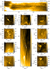 |
Fig. B.1. SDO/AIA 171 Å observations corresponding to the eleven thin coronal jets associated with CBPs shown in Fig. 1. Cases 06 and 09 are those in which the spine of the jet, indicated by the gray arrows, can be easily distinguished in AIA. In the other cases, the jet base may be inferred, or the jet is completely absent. The intensity of the images is given in DN and times are in UT. The images display the same regions as observed by HRIEUV but are not spatially co-aligned, as the goal is to provide contextual information. The AIA times have been selected to match the corresponding HRIEUV observations, accounting for the light travel time delay due to Solar Orbiter’s position near the Sun. Individual movies for each dataset are available . |
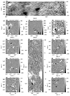 |
Fig. B.2. Line-of-sight photospheric magnetograms from SDO/HMI corresponding to the eleven thin coronal jets associated with CBPs discussed in this paper. The field strength of the images is given in G and times are in UT. The HMI maps were acquired at the time closest to the AIA images shown in Fig. B.1, and have been co-aligned accordingly. |
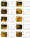 |
Fig. B.3. Widths of narrow coronal jets emanating from CBPs for cases 02 to 11. The red dashed line in the HRIEUV images indicates the Bézier curve that fits the spine of the jet, while the perpendicular blue line marks the cut used to determine the FWHM shown in the adjacent panel. In the 1D plots, the dotted gray lines serve as visual aids to illustrate how the FWHM is determined. |
All Tables
All Figures
|
Fig. 1. Context for the Solar Orbiter HRIEUV observations of the eleven cases showing thin coronal jets (gray arrows) associated with CBPs that are analyzed in this paper. The intensity of the images is given in DN and times are in UT. The details of each observation are provided in Table 1. Individual movies for each of the cases are available online. |
| In the text | |
|
Fig. 2. Analysis of case 01 during the gentle reconnection phase at 05:19:30 UT (top row) and the enhanced phase at 05:44:00 UT (bottom row). Panels a and d show the CBP and the associated thin coronal jets (gray arrows). Panels b and e display space–time maps obtained by taking the maximum intensity along the width, W, of the bent red slit of length L shown in panels a and d, respectively. Panels c and f illustrate the widths of the narrow jets, calculated using the FWHM at L = 7.5 Mm, as indicated by the blue dotted lines in panels a and d, respectively. |
| In the text | |
|
Fig. 3. Plasmoid signatures in case 08. Panel a: Context view showing the CBP and the current sheet within a rectangle of length, L, and width, W. Panel b: Zoomed-in view of the blue rectangle shown in panel a, highlighting the illustrative plasmoid with a cyan arrow. Panel c: Space–time plot of the current sheet, obtained by taking the maximum intensity along the W direction. The cyan dashed line indicates the trajectory of the plasmoid. Panel d: Intensity profiles along the current sheet at different times, illustrating the evolution of the plasmoid indicated in panel c. An animation of this figure is available on zenodo and online, showing the evolution of the plasmoid between 19:10:35 UT and 19:11:10 UT. |
| In the text | |
|
Fig. 4. Same as Figure 3, but for the plasmoid signatures in the 2D CBP simulation by Nóbrega-Siverio & Moreno-Insertis (2022). Top row shows the HRIEUV synthetic emissivity at the original resolution of the numerical experiment (≈16 km). Bottom row shows the results after degrading the resolution to match the best case achievable by HRIEUV in our study (pixel size of 108 km). An animation of this figure is available on zenodo and online, showcasing the plasmoid evolution between t = 29.9 and t = 30.0 min. |
| In the text | |
|
Fig. 5. Indirect signatures of plasmoid-mediated reconnection in case 01. Panel a: Context view illustrating the CBP and the associated ejections. The arrows mark the signatures that are interpreted as consequences of plasmoid-mediated magnetic reconnection. Panel b: Space–time map obtained by sampling the intensity along the slit of length L shown in panel a. Panel c: Intensity profiles along the slit at 05:44:00 UT. An animation of this figure is available online, showing the time evolution between 05:43:48 UT and 05:44:12 UT. |
| In the text | |
|
Fig. 6. Indirect signatures of plasmoid-mediated reconnection in the outflow region from the 2D CBP simulation by Nóbrega-Siverio & Moreno-Insertis (2022) between t = 52.43 and t = 52.60 min. We have transposed the axes so that height appears on the horizontal axis to ease the comparison with the observations. Column (a): Temperature maps. Column (b): nenH, the product of the electron and hydrogen number densities. Column (c): HRIEUV synthetic emissivity at the original resolution of the experiment (≈16 km). The three panels of the top row include the locations of the CBP, the current sheet (CS), and the jet. The arrows 1 and 2 follow the formation and ejection of two different plasmoids along with their signatures in the outflow region. |
| In the text | |
|
Fig. 7. Indirect signatures of plasmoid-mediated reconnection in the outflow region from the 2D CBP simulation by Nóbrega-Siverio & Moreno-Insertis (2022) after degrading the resolution to match the best case achievable by HRIEUV in our study (pixel size of 108 km). Panel a: HRIEUV synthetic emissivity. We have transposed the axes so that height appears on the horizontal axis. Panel b: Space–time map obtained by sampling the intensity along the slit of length L shown in panel a. Panel c: Intensity profiles along the slit at t = 52.60 min. In all the panels, the arrows mark some of the features that are interpreted as consequences of plasmoids previously ejected during the reconnection process. An animation of this figure is available online, including temperature and nenH maps, showcasing the appearance of indirect plasmoid-mediated signatures between t = 52.40 and t = 52.80 min. |
| In the text | |
|
Fig. B.1. SDO/AIA 171 Å observations corresponding to the eleven thin coronal jets associated with CBPs shown in Fig. 1. Cases 06 and 09 are those in which the spine of the jet, indicated by the gray arrows, can be easily distinguished in AIA. In the other cases, the jet base may be inferred, or the jet is completely absent. The intensity of the images is given in DN and times are in UT. The images display the same regions as observed by HRIEUV but are not spatially co-aligned, as the goal is to provide contextual information. The AIA times have been selected to match the corresponding HRIEUV observations, accounting for the light travel time delay due to Solar Orbiter’s position near the Sun. Individual movies for each dataset are available . |
| In the text | |
|
Fig. B.2. Line-of-sight photospheric magnetograms from SDO/HMI corresponding to the eleven thin coronal jets associated with CBPs discussed in this paper. The field strength of the images is given in G and times are in UT. The HMI maps were acquired at the time closest to the AIA images shown in Fig. B.1, and have been co-aligned accordingly. |
| In the text | |
|
Fig. B.3. Widths of narrow coronal jets emanating from CBPs for cases 02 to 11. The red dashed line in the HRIEUV images indicates the Bézier curve that fits the spine of the jet, while the perpendicular blue line marks the cut used to determine the FWHM shown in the adjacent panel. In the 1D plots, the dotted gray lines serve as visual aids to illustrate how the FWHM is determined. |
| In the text | |
Current usage metrics show cumulative count of Article Views (full-text article views including HTML views, PDF and ePub downloads, according to the available data) and Abstracts Views on Vision4Press platform.
Data correspond to usage on the plateform after 2015. The current usage metrics is available 48-96 hours after online publication and is updated daily on week days.
Initial download of the metrics may take a while.