| Issue |
A&A
Volume 702, October 2025
|
|
|---|---|---|
| Article Number | A198 | |
| Number of page(s) | 12 | |
| Section | The Sun and the Heliosphere | |
| DOI | https://doi.org/10.1051/0004-6361/202555368 | |
| Published online | 21 October 2025 | |
Characterizing solar wind electrons with the core-strahlo model: WIND-SWE-VEIS observations
1
Departamento de Física, Facultad de Ciencias, Universidad de Chile, Santiago, Chile
2
Departamento de Fisica, Universidad de Santiago de Chile, Santiago, Chile
3
Center for Interdisciplinary Research in Astrophysics and Space Sciences (CIRAS), USACH, Santiago, Chile
4
Centro de Instrumentacion Cientifica, Universidad Adventista de Chile, Chillan, Chile
5
Centre for Mathematical Plasma Astrophysics, Department of Mathematics, KU Leuven, Celestijnenlaan 200B, B-3001 Leuven, Belgium
6
Institute for Theoretical Physics IV, Faculty for Physics and Astronomy, Ruhr-University Bochum, D-44780 Bochum, Germany
7
Department of Physics & the Institute for Astrophysics and Computational Sciences (IACS), Catholic University of America, Washington-DC 20064, USA
8
NASA Goddard Space Flight Center, Emeritus Scientist, Heliospheric Science Division, Mail Code 673, Greenbelt, MD 20771, USA
⋆ Corresponding authors: This email address is being protected from spambots. You need JavaScript enabled to view it.
; This email address is being protected from spambots. You need JavaScript enabled to view it.
Received:
2
May
2025
Accepted:
13
September
2025
Abstract
Context. In this study, we apply a novel heuristic core-strahlo (CS) model to analyze solar wind electrons. This model reproduces the behavior of a core-halo-strahl representation by employing solely two subpopulations: a bi-Maxwellian core and a modified Kappa distribution that introduces skewness. This modification effectively represents halo and strahl electrons within a single skew distribution.
Aims. This work aims to demonstrate that the CS model can be utilized to model observations beyond theoretical contexts. The CS model can reproduce the main features of electron velocity distribution functions (eVDFs) in the solar wind–thermal core, enhanced tails, and skewness–with the advantage that a single parameter controls the asymmetry.
Methods. We implemented a comprehensive statistical analysis of solar wind electrons at 1 AU using the electron and solar wind plasma moments on board the NASA Wind SWE/VEIS instrument. This work uses a sophisticated algorithm developed to analyze and characterize separately the core and strahlo populations. We limited our effective energy from 10 eV to 3 keV and fit the eVDFs measurements observed by the WIND satellite to the CS model.
Results. Our experimental analysis show good agreement with existing models of solar wind electrons, including those that account for core, halo, and strahl components, as the resulting values fall within the expected order of magnitude. The CS model not only achieves results comparable to previous studies, but also offers the added capability of accounting for heat flux and the asymmetry of the electron velocity distribution through the δ parameter, which enhances our understanding of solar wind electron dynamics. Further, we confirm that the kappa parameter (κ) is independent of the skewness parameter (δ), consistent with previous theoretical studies’ findings.
Conclusions. This work serves as an initial practical application of the CS model. We extend its relevance beyond theoretical contexts to the study of observational data. This novel approach not only highlights the specific dynamics of solar wind electrons but also provides insights into their behavior. Specifically, as the strahl relaxes, the halo becomes more enhanced.
Key words: plasmas / Sun: heliosphere / solar wind
© The Authors 2025
 Open Access article, published by EDP Sciences, under the terms of the Creative Commons Attribution License (https://creativecommons.org/licenses/by/4.0), which permits unrestricted use, distribution, and reproduction in any medium, provided the original work is properly cited.
This article is published in open access under the Subscribe to Open model. This email address is being protected from spambots. You need JavaScript enabled to view it. to support open access publication.
1. Introduction
The solar wind is a weakly collisional plasma originating from the Sun and extending across space. In such low-collisionality systems, Coulomb collisions are insufficient to drive particle populations toward thermal equilibrium. Thus, the velocity distributions of particles may depart from standard Maxwellian functions, which characterizes the equilibrium state. These deviations, referred to as nonthermal or suprathermal features, have been extensively documented in observational studies for the solar wind plasma’s electrons and ions. Notable features systematically observed in electron velocity distributions include power-law high-energy tails and magnetic field-aligned skewness, along with a quasithermal core at low energies (Feldman et al. 1975; Pilipp et al. 1987a; Nieves-Chinchilla & Viñas 2008).
These nonequilibrium electron distributions have been empirically interpreted in terms of three distinct subpopulations: core, halo, and strahl. This structural framework is widely accepted for characterizing the observed electron distributions and their suprathermal attributes in the solar wind (Maksimovic et al. 1997; Pierrard et al. 2001; Štverák et al. 2008; Pierrard et al. 2016; Tao et al. 2016; Wilson et al. 2019a,b). Commonly measured at low energies (up to a few tens of electronvolts), the quasithermal core subpopulation constitutes the majority of solar wind electrons, accounting for over 90% of the total number density. This dominant and dense population is often best described by bi-Maxwellian velocity distributions. However, a recent approach utilizing bi-self-similar functions has emerged to model the core segment of observed electron distributions in interplanetary shocks near 1 AU. This approach demonstrates that a self-similar velocity distribution function provides a more accurate description of the core subpopulation than a standard bi-Maxwellian (Wilson et al. 2019a,b). Next, the halo subpopulation is observed at higher energies, often ranging up to a few keV. These electrons are distributed across all pitch angles and are responsible for the characteristic power-law energetic tails of electron distributions. Historically, bi-Maxwellian functions with lower amplitudes and higher temperatures than those of the core were commonly utilized to perform fittings and emulate the energetic tails in the early works (Pilipp et al. 1987b; Feldman et al. 1975). However, more recent studies have shown that bi-Kappa distribution functions better describe this specific subpopulation (Maksimovic et al. 2005; Štverák et al. 2009). Lastly, the strahl subpopulation constitutes a suprathermal beaming component, generally more pronounced in the fast wind, primarily moving antisunward and parallel or antiparallel to the magnetic field direction. This component imparts the characteristic skewness to the electron velocity distributions. While efforts have been made to fit this observed population using a proper analytical expression (Štverák et al. 2009; Horaites et al. 2017; Abraham et al. 2022), there is no current consensus regarding such best analytical form and the most commonly used approach for incorporating the skewness into theoretical works is by considering drifting distributions. This categorization and separation of the total electron distribution (sectioning) into three distinct subpopulations is not only an observational tool used to characterize the distributions. It is believed that the dominant processes governing their formation and, thus, their shape in velocity space are different for each subpopulation and their evolutionary dynamics from the solar corona throughout the heliosphere (Pierrard et al. 1999; Vocks et al. 2005; Owens et al. 2008; Štverák et al. 2009; Pavan et al. 2013; Pavan & Viñas 2019; Wilson et al. 2019a,b). The quasithermal shape of the low energy core is usually attributed to Coulomb collisions, considering the high dependence of Coulomb collision mean free path on velocity. Thus, this low-energy component is the distribution portion where Coulomb collisions remain essential (Scudder & Olbert 1979; Landi et al. 2012; Pilipp et al. 1987b).
On the other hand, it is widely recognized that Coulomb collisions are largely ineffective for strahl electrons due to their higher energies, which enables many to escape the solar corona with minimum interaction (Wilson et al. 2019a). As these electrons move away from the Sun, magnetic focusing tends to narrow their pitch-angle distribution due to the decreasing intensity of the magnetic field. Nevertheless, this focusing effect is mitigated by other pitch-angle scattering mechanisms, such as wave–particle interactions, turbulence, and residual collisions, which broaden the strahl and disrupt the conservation of the first adiabatic invariant (i.e., the magnetic moment). Numerous studies have shown that the magnetic moment is not conserved for strahl electrons in the solar wind, which highlights the significance of these non-adiabatic effects (e.g., Bercic et al. (2019), Horaites et al. (2018)). Understanding the relative contributions of these systems in heliospheric physics remains an open question.
Numerous studies have aimed to characterize these out-of-equilibrium electron distributions and their suprathermal nature from an observational perspective. Some of these investigations focus on fitting analytical models, which predominantly, but not exclusively, involve bi-Maxwellian and bi-Kappa functions (Maksimovic et al. 1997, 2005; Štverák et al. 2008; Pierrard et al. 2016; Wilson et al. 2019a,b). Through these fits, we can obtain and estimate important parameters for the electron subpopulations, such as number densities, kinetic temperatures, and heat flux moment. Obtaining these parameters allows us to characterize the observed electron distributions, quantify their departure from equilibrium, and analyze how the distributions change and evolve throughout the heliosphere in a more manageable way. This has been of crucial importance in understanding their variability and also their dependence on relevant factors such as radial distance, solar cycle, and plasma velocity, among others (Maksimovic et al. 2005; Štverák et al. 2009; Lazar et al. 2020). Additionally, understanding the temporal and spatial evolution of these parameters can help us discern the importance of kinetic processes, whether collisional or non-collisional, for the solar wind electron dynamics (Bale et al. 2013; Horaites et al. 2015; Halekas et al. 2020, 2021; Landi et al. 2014; Pavan et al. 2013; Pavan & Viñas 2019).
A crucial insight using this kind of procedure is the radial evolution and interplay between electron suprathermal subpopulations and comes from the work of Maksimovic et al. (2005). Through a procedure involving the modeling of distributions observed by Helios, Wind, and Ulysses spacecraft in fast solar wind conditions, the authors calculated the relative number density of core, halo, and strahl components for a range of heliocentric distances spanning from 0.3 to 1.5 AU. They showed that the relative number of the halo subpopulation increases as we move away from the Sun, while the strahl electrons exhibit the opposite behavior. This occurs while maintaining the core density almost unchanged. This fact provided first-time data evidence suggesting that the halo is partially formed at the expense of scattered strahl electrons as the solar wind expands from the outer solar corona into the heliosphere. This conclusion is widely accepted and has received additional support from observations. For instance, by utilizing data from Helios, Cluster II, and Ulysses in the ecliptic plane, Štverák et al. (2009), Gurgiolo et al. (2012) confirmed the trend of opposite variation in suprathermal electron density with radial distance. Furthermore, they extended this conclusion to even greater distances, reaching up to 4 AU and encompassing the slow solar wind regime. The exact mechanism for the scattering of strahl electrons still needs to be completely understood. However, in the absence of collision the self induced instabilities may be an important process to consider (Zenteno-Quinteros et al. 2021; Zenteno-Quinteros & Moya 2022).
A recent study by Zenteno-Quinteros et al. (2021) introduced a novel depiction of the electron population in the solar wind. The authors propose the core-strahlo (CS) model as an innovative approach for characterizing the solar wind electrons. This model utilizes a heuristic dual-population technique to accurately represent the intricate nature of observed solar wind electron distributions, effectively qualitatively reproducing their key attributes. The CS description uses the typical (bi-)Maxwellian distribution to represent the core population, which is present at low energies but has a higher density.
In addition, CS model relies on the skew-Kappa function to mimic the observed skewness and high energy tails, leading to a unified analytical description of both the halo and Strahl kinetic attributes. This population was referred to as “strahlo”, considering that it combines the suprathermal components, strahl and halo. So far, the CS model has primarily served as a theoretical tool for studying electron dynamics at kinetic scales. In this context, the CS representation has successfully reproduced outcomes achieved by well-established models for the solar wind electron population, such as drifting bi-Maxwellians (Zenteno-Quinteros et al. 2021; Zenteno-Quinteros & Moya 2022; Zenteno-Quinteros et al. 2023). This agreement with previous research on linear stability analysis provides significant theoretical validation for the CS model. Thus, this approach could be useful for studying and understanding the intricate dynamics of the interaction between these suprathermal populations, especially in intermediate states specifically, during the formation or relaxation of the electron strahl, when it is more intimately linked to the halo.
As mentioned earlier, the current approach of the CS framework has been focused solely on theoretical work. However, an analysis of its applicability from an observational perspective has yet to be conducted, and if it can eventually be established as a suitable representation of the solar wind eVDF. Thus, this work aims to demonstrate that the CS model can be utilized to model observations beyond theoretical contexts. Specifically, to offer observational support to the CS approach by conducting a fitting procedure of the model to electron distributions observed by the WIND satellite in the pristine solar wind. This pursuit is particularly significant due to the model’s capability to describe both the halo and strahl subpopulations analytically and aims to complement the previous theoretical validation of the CS description. In this paper, we show that such a skewed Kappa distribution can be applied to describe the asymmetric suprathermal component of the electrons near 1 AU.
So, this article is structured as follows: In Section 2, we provide a detailed description of the instruments and dataset used in this work, present an overview of the CS model, and explain the procedure used for data fitting. In Section 3, we present and discuss our fitting results. Furthermore, we present the summary and discussion in Section 4, and finally, Section 5 is dedicated to conclusions.
2. Instrumentation and data analysis method
2.1. Data
In this study, we utilize solar wind electron measurements and magnetic field vectors from NASA’s Wind mission instruments. Our dataset comprises the magnetic field data with a spin resolution of 3s from the Magnetic Field Investigation (MFI) (Lepping et al. 1995). In addition, we use the electron moments derived from the velocity moments integration of solar wind electron distributions energy, as well as pitch angle electron distributions (fobs(E, μ)), where E is the electron kinetic energy and μ = cos θ is the pitch angle between the electron velocity vector and the magnetic field. These distributions are derived from three-dimensional electron particle measurements obtained from the 3s time resolution data of the Wind SWE/VEIS instrument, as described by Ogilvie et al. (1995). This instrument consists of two sets of three small electrostatic analyzers, each featuring a deflection angle of 127°. It was designed to determine the distribution functions of ions and electrons within an energy range of 7 eV to 24.8 keV. This range was divided into 16 energy steps, with an energy resolution of approximately 6%. For the context of solar wind electron studies, the effective energy range is limited to 10 eV to 3 keV. The computation of energy-pitch angle distributions involves 3-second time-resolution data from the three-dimensional electron distribution measurements, with temporal intervals of either 6 or 12 seconds. All measurements used in this study were averaged over 1-minute intervals to ensure consistency and reduce noise. The observations obtained at each energy channel are categorized into pitch-angle bins spanning six degrees each. Consequently, there are 30 pitch angle bins covering the range from 0° to 180° degrees with respect to the local magnetic field. To apply the CS model to observational analysis, we have selected measurements from May 15, 1995, to July 3, 1995. During this period, the WIND spacecraft was located near its first apogee, near the L1 Lagrange point. This time frame corresponds to the period analyzed in the study of Salem et al. (2003). The decision to use the same period is motivated by the absence of magnetic clouds or significant interplanetary shocks corresponding to quiet solar wind conditions (Salem et al. 2003; Sanderson et al. 1998). Moreover, within this 50-day window, both fast and slow solar wind intervals are observed, which provides an opportunity to assess the model’s applicability under varying solar wind conditions.
2.2. Spacecraft potential
In our study, we process the satellite data and correct the measured electron distribution. This correction is necessary to avoid cold photo-electrons from the spacecraft body, contaminating the measurements at low-energy bins. Hence, to ensure a precise depiction of solar wind electrons, we differentiate between the actual electron measurements originating from the solar wind and those potentially influenced by the photoelectric effect. As a result, we exclude data from the analysis that corresponds to the two lowest energy channels (13.923 eV and 20.112 eV). This procedure guarantees that in most of our samples, the retained measurements are mainly associated with solar wind electrons, effectively eliminating the contaminated part of the distribution. Further, we correct the effects of the spacecraft potential on the measured eVDFs by performing a scalar adjustment. This correction involves deducting the estimated energy associated with the spacecraft’s electric potential from each energy channel.
2.3. The CS model
We use the CS distribution shown in Equation (1) to describe the electron velocity distributions observed in the solar wind. The electron population description method, proposed in Zenteno-Quinteros et al. (2021), is an analytical and heuristic method for modeling electrons in theoretical contexts. In our investigation, we adopt this description as an analytical fitting model to provide observable evidence for its applicability in space plasma context. The CS model combines two populations to depict the solar wind electron distribution function fe. This description involves the superposition of a bi-Maxwellian distribution, denoted as fc, and a skew-Kappa function, denoted as fs, to characterize the quasithermal core and strahlo subpopulations, respectively. These mathematical expressions can be seen in Equations (1) through (3). Combining only two functions, the CS model qualitatively reproduces three significant non-thermal features observed in solar wind electron distributions: the quasi-thermal core, high-energy tails, and field-aligned skewness, as demonstrated in previous research. We fit the observed eVDFs with the sum of two analytical expressions that separately describe each of the electron populations, namely the core and strahlo:
 (1)
(1)
where fc(v⊥, v∥) is the fitted core defined as
 (2)
(2)
fs(v⊥, v∥) is the fitted strahlo defined as
![Mathematical equation: $$ \begin{aligned} f_{s}(v_{\perp }, v_{\parallel })&= n_sC_{s}\left[1+ \frac{1}{\kappa - \frac{3}{2}}\left(\frac{v_{\bot }^2}{\theta _{\bot }^2} + \frac{(v_{\parallel } - U_{s})^2}{\theta _{\parallel }^2} \right.\right. \nonumber \\&\left.\left. + \delta \left( \frac{(v_{\parallel } - U_{s})}{\theta _{\parallel }} - \frac{(v_{\parallel } - U_{s})^{3}}{3\theta _{\parallel }^3}\right)\right)\right]^{-(\kappa +1)}, \end{aligned} $$](/articles/aa/full_html/2025/10/aa55368-25/aa55368-25-eq3.gif) (3)
(3)
![Mathematical equation: $$ \begin{aligned} C_s = \dfrac{\Gamma (\kappa +1)}{\left[(\kappa - \frac{3}{2})\pi \right]^{3/2}\theta _{\perp }^2\theta _{\parallel }\Gamma (\kappa - \frac{1}{2})} \left[1-\frac{\delta ^2}{4}\Upsilon _1(\kappa )\right], \end{aligned} $$](/articles/aa/full_html/2025/10/aa55368-25/aa55368-25-eq4.gif) (4)
(4)
and
 (5)
(5)
In the aforementioned equations, the subscripts ∥ and ⊥ denote the directions parallel and perpendicular to the background magnetic field B0. The parameters α∥, ⊥ represent the core thermal speed, θ∥, ⊥ are values associated with the strahlo kinetic temperatures, but expressed in units of speed. Additionally, nc and ns denote the number densities of the core and strahlo populations respectively, Uc and Us represent the core and strahlo drift velocities, δ and κ are dimensionless parameters controlling the skewness and energetic tails of the distribution. Furthermore, Cs serves as a normalization constant, which ensures that ns = ∫fs d3v. It is important to note that for fs to serve as an appropriate distribution function for the solar wind’s electrons, both in theoretical and observational contexts, its applicability must be limited to cases of small skewness, specifically where |δ|< 1. A comprehensive discussion of this validity range and associated mathematical details can be found in Zenteno-Quinteros et al. (2021). Under this assumption, the normalization constant Cs is given by Eq. (4). The CS model must also satisfy quasi-neutrality and zero net current conditions expressed in Eqs. (6) and (7), within the model’s validity range.
 (6)
(6)
Here, np denotes the proton density, which ensures charge neutrality in the plasma.
 (7)
(7)
Given the restriction |δ|< 1, the skew-Kappa function fs, as demonstrated in prior studies, effectively captures the skewness and high-energy tails present in the observed electron distributions in the solar wind. Thus, it qualitatively reproduces the kinetic characteristics empirically associated with two distinct subpopulations–the halo and the strahl. Namely, high-energy tails and skewness, respectively.
2.4. Fitting procedure of observed eVDF
Upon removing spacecraft potential, we transform the observed electron distribution samples from energy and pitch angle space (fobs(E, α)) to velocity space (fobs(v⊥, v∥)), where v⊥, ∥ represent velocity components relative to the background magnetic field. To perform an observational test on the CS model, we employ reduced versions of the distribution (Eq. (1)) rather than the full 2-D distribution. This approach is motivated by the anticipation that suprathermal tails will easily form in the parallel direction due to the electrons’ unrestricted movement along the magnetic field lines, as well as the consistent alignment of the strahl with the magnetic field. Moreover, the reduced distribution offers a more convenient visual representation of the quality of the fits. The reduction process involves transforming the original 2-D distributions into the (v⊥, v∥) space using the measured 3 s magnetic field averages and then integrating the 2-D distributions in the perpendicular direction. This process yields 1-D distributions that accurately represent the component along the magnetic field. The reduced distributions are denoted as
 (8)
(8)
and
 (9)
(9)
These reduced distributions are functions of a single variable, which describes electron behavior in relation to the background magnetic field. These single-variable distributions are then fitted to the empirical data obtained from WIND. It is important to note that even if the 1D reduced distributions provide an accurate representation of the data and can be matched exactly by the 1D CS model, the actual 2D distributions might still differ from the 2D CS model. This caveat should be kept in mind when interpreting the results. Bearing this limitation in mind, the next step involves applying the fitting technique to the reduced parallel distribution.
By employing the zero current condition mentioned earlier, this fitting technique in f∥ yields optimal parameter values for δ, κ, nc, ns, α∥, θ∥, Uc and Us. Next, we repeat this procedure for f⊥. We obtain the best-fit values for the remaining parameters: θ⊥ and α⊥. Altogether, we obtain ten relevant fit parameters of the CS distribution. Since the reduced analytical functions exhibit nonlinear dependence on these fitting parameters, we employ an iterative Levenberg-Marquardt algorithm (Marquardt 1963) to address the non-linear least squares curve-fitting challenge effectively. To visualize the quality of the fitting analysis, we present plots in Figure 1 that display the typical reduced eVDFs data (i.e., red asterisks) superposed with the core strahlo model (i.e., solid black line). The upper panel in Figure 1 shows an eVDF obtained for the parallel fits, while the bottom panels represent the perpendicular fit. This visual representation serves as a measure of how well the reduced chi-square χ2 function for eVDFs has been minimized, indicating the goodness-of-fit. Then, to find intervals of good fit, we employ the following multi-step data selection process. First, we ensure only fits that produced χ2 < 1 were considered (where χ2 is the χ2 per degrees of freedom of the fit). While χ2 < 1 can theoretically indicate overfitting, where the model improperly fits noise or error variances are overestimated. This threshold is frequently observed in helio physics data analysis [see (Salem et al. 2023)]. In our case, χ2 < 1 threshold excludes cases in which the adjusted curve did not well represent the data.
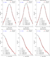 |
Fig. 1. Typical reduced electron velocity distribution functions (eVDFs) measured by the Wind Solar Wind Experiment (Wind/SWE-VEIS) at 1 AU in the slow solar wind. The top and bottom panels represent the eVDF in the parallel (∥) and perpendicular (⊥) directions relative to the magnetic field (B), respectively. The red stars indicate the eVDF data, while the solid black line represents the fitted distribution, which is a superposition of a bi-Maxwellian distribution and a skew-Kappa function used to initialize the eVDF fit. Each panel includes key fit parameters and the chi-square (χ2) value obtained from the fit. |
Second, we implemented a data selection criterion based on the ratio of the total density (nT = nc + ns) obtained from the fit to the density observed from the WIND mission (ne). This ratio, defined as ζ = nT/ne, was used to filter the dataset by identifying and removing extreme outliers that could distort the analysis. Approximately 8.5% of the data points were excluded based on a ζ threshold, and an additional 12% were removed based on a reduced chi-squared threshold.
Further, we employed the interquartile range (IQR) method to establish thresholds for outlier exclusion. Precisely, the first (Q1) and third (Q3) quartiles of the ζ distribution were calculated, and the IQR was determined as the difference between Q3 and Q1. We set lower and upper bounds to identify potential outliers at Q1 − 3.0 × IQR and Q3 + 3.0 × IQR, respectively. Data points with ζ values falling outside these bounds were excluded from the dataset. This filtering method was selected because it effectively removes the impact of extreme values. Hence, we focus the analysis on the range of ζ values that are physically reasonable and representative of the typical behavior in the solar wind. By applying these thresholds, we retained data points that provide a reliable and meaningful insight into the relationship between the core and strahlo components of the electron velocity distributions. We also restrict the parameter δ to the range of −0.4 to 0.4 to ensure that fs remains a valid distribution function for the solar wind’s electrons in both theoretical and observational contexts. This restriction limits the applicability to cases of slight skewness, specifically where |δ|< 1 (Zenteno-Quinteros et al. 2021). Another restriction we impose is the kappa parameter (κ) within the 1.5 < κ ≤ 30 range, aligning with established values observed in previous solar wind electron distribution studies. Finally, we restricted ns within the 0.1 to 1.0 cm−3 range.
3. Statistical results of the CS model fitting to the observed eVDF
In this section, we present the statistical analysis results described in the previous section. Overall, we examine 65,850 electron velocity distribution functions collected by the WIND mission over a period of 50 days. The restrictions procedure outlined in Subsection 2.4 yields a subset of data containing ∼27 215 samples for further analysis. Out of the 27 215 samples, 16 860 samples are classified as slow wind (Vsw ≤ 500 km s−1 ), and 10 335 are classified as fast wind (Vsw ≥ 500 km s−1. For each of these two populations, we compute the statistical values for fit and solar wind parameters. The statistical values are presented in Tables A.1 to A.3 for the whole data set, slow solar wind, and fast solar wind, respectively. Figure 2 shows an example of a time series for solar wind and CS fit parameters for slow and fast wind, respectively. To assess the quality of the fits, we present in Figure 3 the joint 2D histogram plot that compares the estimated total density (nT) from CS fits against the total moment density provided by the Wind mission (ne). Notice the linear relationship between nT as a function of ne, which demonstrates the reliability of the fits and the robustness of the imposed constraints. Notably, most of the data points are clustered around the 1:1 identity relation (solid black line), which indicates strong agreement between the estimated and observed densities. This serves as a quality control measure for the data under analysis. Additionally, marginal (1D) histograms display the occurrence frequency of nT over the 50-day interval in 1995 at the top, while those for ne are shown on the right of Figure 3. To statistically analyze solar wind electron data at 1 AU, we utilize various visualization methods, which are presented in the following subsection. This subsection also introduces the first statistical analysis of the CS fit parameters.
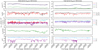 |
Fig. 2. Time series plots of solar wind and CS fit parameters. The left panels correspond to the slow solar wind observed on June 10, 1995, while the right panels correspond to the fast solar wind observed on June 1, 1995. The top panels for both fast and slow wind show the time series of densities (cm−3). The second panel from the top presents the time series of the heat flux. The third panel displays the time series of the thermal velocities. The fourth panel illustrates the solar wind speed. The bottom panel shows the time series of kappa and delta. |
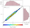 |
Fig. 3. Joint (2D) histograms which compares the total electron density (nT = nc + ns) estimated from CS fits with the total moment electron density (ne), over a 50-day interval in 1995. The solid black line denotes the 1:1 identity relation, and the color scale represents the logarithm of the count number in each bin. Marginal (1D) histograms show the occurrence frequency of nT (top) and ne (right). The axis limits for both nT and ne have been selected to capture the bulk of the data while excluding extreme outliers. |
3.1. Statistics of core and strahlo components
We investigated the distributions of the parameters obtained from our fit results to understand their respective trends and how they compare. To guarantee accurate alignment of both histograms, we use common bin edges for the 2D color plots with respect to the data range. The column-normalized histograms in Figure 4 depict the core density (nc) as a function of strahlo density (ns) for both slow (left panel) and fast (right panel) wind in our data set. These histograms exhibit a linear correlation. For ns ≥ 0.2 cm−3, the value of ns increases as nc increases, implying a balance in their ratio. Hence, the percentage of each of them is a stable quantity in the solar wind at 1 au from the Sun. For cases where ns ≤ 0.2 cm−3, the nc is large, but there is no strahlo.
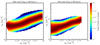 |
Fig. 4. Normalized distribution of the core electron density, (nc cm3) and the strahlo electron density (ns cm3) for slow (left panel) and fast wind (right panel). The color bar represents the logarithm of the number of counts per bin, normalized to the maximum number of counts per bin in each column. The black circles mark the peak centroid in each column, and the black vertical lines represent the half-width or standard deviation based on a Gaussian fit to the normalized values in each column. |
Nonetheless, our observational results show good agreement with existing models of solar wind electrons, including those that account for core, halo, and strahl components, as the resulting values of nc and ns fall within the expected order of magnitude (See Maksimovic et al. 2005; Nieves-Chinchilla & Viñas 2008; Lazar et al. 2020; Pierrard et al. 2022). The densities and density ratio statistics for all slow and fast solar wind conditions, respectively, are presented in Tables A.1 to A.3.
Figure 5 shows the probability density plot of the available measurements for each value of core thermal velocity and strahlo θ parameter along the magnetic field direction, denoted as α∥ and θ∥. This probability was calculated as the number of measurements available NM in a given bin divided by the total number of measurements NT, and divided by the area of the bin (which is variable due to the logarithmic scale). Each panel in the figure was divided into cells of size 0.01 × 0.01 (in a log–log scale), corresponding to a bin area of Abin = 10−4. Each cell was colored only if the normalized count density satisfied:  . Similar to the case of number density, the observed values for both components are consistent with the ranges reported in previous studies based on the core and halo distributions (Pierrard et al. 2022; Lazar et al. 2020). The probability density plot reveals that, for small values of θ∥, α∥ can take on a wide range of values. In contrast, when α∥ is small, the value of θ∥ also tends to be small. For large values of α∥, the value of θ∥ is not strongly constrained and can vary significantly. This observation clearly shows a non-linear relationship between the two parameters. In the right panel of Figure 5, we present a probability density plot for the available measurements of the core thermal velocity and strahlo θ parameter in the perpendicular direction, denoted as α⊥ and θ⊥, respectively. In contrast to the parallel direction, the relationship between α⊥ and θ⊥ exhibits a linear correlation. This typically suggests that the thermal energy of these components is interconnected or influenced by similar physical processes. We assume that this relation indicates that both the core and strahlo components undergo similar heating processes, such as wave-particle interactions, plasma expansion, or perpendicular diffusion processes in the solar wind. We attribute the apparent boundary in the figure for both for parallel and perpendicular directions to a lack of data points beyond certain ranges rather than a strict physical constraint.
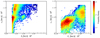 |
Fig. 5. Probability density plots of the core thermal velocity (α) versus strahlo θ parameter. The left panel represents the velocities along the parallel direction, while the right panel corresponds to the perpendicular direction. Each point represents the 1-minute over the 50-day interval in 1995. |
3.2. Strahlo properties
Here, we present the results obtained for the properties of Strahlo electrons. Figure 6 illustrates the relationship between the θ∥, and the kappa parameter (κ). The results of our study establish a clear correlation between these variables: a higher value of κ is associated with a higher θ∥, and conversely, an increased θ∥ is also associated with a higher value of κ. While this relation is not strictly one-to-one, the observed correlation is noteworthy. This observation is consistent with the findings of Olbert (1995), Tao et al. (2016, 2021), Lazar et al. (2017), demonstrating that the effective temperature depends on κ. This has also been theoretically studied by Lazar et al. (2015, 2016), Daniel et al. (2024).
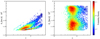 |
Fig. 6. Probability density plot illustrating the relationship between the spectral index parameter (κ) and the electron thermal velocity (θ∥). The left panel represents the parallel direction, while the right panel corresponds to the perpendicular direction. The binning scheme employs logarithmically spaced bins with a step size of 0.01, and cells are colored only if NM/NT > 10−5. |
In contrast, the analysis of the θ⊥, and κ, as shown in the right panel of Figure 6, did not reveal any significant relationship between these parameters. Figure 7 shows the relationship between the κ and δ non-thermal parameters. As mentioned, the δ parameter, which is directly related to the skewness of the distribution, ranges from -0.4 and 0.4. Furthermore, the κ parameter, which describes the suprathermal tail of the distribution, varies from 1.8 to 30.
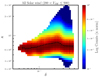 |
Fig. 7. Normalized distribution of kappa versus delta parameter. The color bar represents the logarithm of the number of counts per bin, normalized to the maximum number of counts per bin in each column. The black circles mark the peak centroid in each column, and the black vertical lines represent the half-width or standard deviation based on a Gaussian fit to the normalized values in each column. |
Moreover, our observation shows that a small value of δ results in a somewhat narrow range in κ. Conversely, a large value of δ allows κ to span a wide range of values. It is evident from the figure that there is no clear dependence between the κ and δ parameters, as most of the data lies in a narrow interval as shown in Figure 7, which is consistent with the theoretical arguments exposed by Beck (2000), which suggest that the skewness parameter should not exhibit a dependence on the κ but rather on the Reynolds number, specifically following the relation,  . This is also consistent with the numerical simulation by Gallo-Méndez & Moya (2023) which found the same lack of dependence between the skewness and high energy tails in a Skew-Kappa distribution.
Figure 8 illustrates the relation between the heat flux (qe∥fit/q0) obtained from the CS fit and δ parameter under both slow and fast solar wind conditions. The parallel heat flux (qe∥fit) is calculated as described by Zenteno-Quinteros et al. (2021):
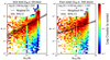 |
Fig. 8. Column-normalized 2D histograms showing the relationship between the δ parameter and the parallel electron heat flux qe∥fit/q0) obtained from the CS fits, for slow solar wind (left panel) and fast solar wind (right panel). The color scale indicates the logarithm of the normalized bin counts. The dashed black line represents a weighted linear regression in log-log space, fitted using 2D histogram counts as statistical weights. The shaded region denotes the 95% confidence interval of the fit. The equation of the fitted relation is displayed in the top-left corner of each panel. |
![Mathematical equation: $$ \begin{aligned} q_{e\parallel _{\rm fit}} = \frac{m_e n_s \theta ^{3}_{\parallel }}{4} \delta _s \left[ \mu _s \Psi _6 (\kappa _s) + \Psi _7 (\kappa _s) + \frac{1}{4} \frac{\alpha ^{2}_{\parallel }}{\theta ^{2}_{\parallel }} (3 + 2 \mu _c) \right] , \end{aligned} $$](/articles/aa/full_html/2025/10/aa55368-25/aa55368-25-eq12.gif) (10)
(10)
where
 (11)
(11)
and
 (12)
(12)
The normalization constant q0 is defined as
 (13)
(13)
We observe a strong correlation between these variables, for slow and fast solar wind conditions. This trend may be coarsely approximated by a linear relation, which affirms the internal consistency between them. The statistical values of all fit and solar wind parameters for all solar wind, slow wind, and fast wind are presented in Tables A.1 to A.3, respectively.
4. Summary and discussion
We applied the CS model to a 50-day data set of NASA Wind SWE/VEIS observations at 1 AU. We use our fitting results to investigate the relation between CS fit parameters and identify general trends among them. The results obtained are entirely novel, and because of the extensive data collected, the overall patterns still need to be clarified. As this is the first study of its kind, all findings and observations are new. Our analysis reveals a strong positive correlation between core and strahlo densities. More importantly, we found that the core accounts for 90%–95% of the total local electron density, which is consistent with previous findings by Maksimovic et al. (2005). According to Maksimovic et al. (2005), the Maxwellian nature of the core is attributed to collisional processes near the Sun, which dominate at lower energies. At higher energies, where collisions are less effective, nonthermal structures such as beams and high-energy tails can develop and persist. The strahlo population represents electrons in the suprathermal energy range, accelerated along magnetic field lines and pitch-angle scattered to all directions. With this process, the higher-energy tails develop in all directions, but skewness remains along the field line. Furthermore, the linear relationship observed between ns and nc is consistent with previous studies of Pierrard et al. (2022), Tao et al. (2016, 2021). However, it is important to note that our research investigates the core and strahlo populations, whereas Tao et al. (2016, 2021) focuses on the components of halo and strahl. In contrast, Pierrard et al. (2022) focused on the core and halo components.
Another key finding from our analysis is the observed linear correlation between α⊥ and θ⊥. In the perpendicular direction, the strahlo behaves similarly to the tail of the core distribution. However, in the parallel direction, the relationship between α∥ and θ∥ is unclear due to underlying phenomenology.
One of the most significant results of our observation is the positive linear correlation between θ∥ and κ. This suggests that broader parallel strahls tend to be associated with distributions that have weaker suprathermal tails (i.e., smaller deviations from Maxwellian behavior). A similar result has already been presented by Tao et al. (2016, 2021). They reported several notable correlations between various parameters related to the halo and the strahl by fitting WIND electron measurements at energies up to 1.5 keV at 1 AU. In particular, they found a strong positive correlation between the kappa parameter (κ) fitted and the effective temperature (Teff). This correlation was attributed to the generation process of strahl electrons at the Sun. Our result is consistent with previous studies by Tao et al. (2016, 2021). Although our fitting approach differs due to the application of a different functional model, the findings are qualitatively the same. In contrast, we do not observe any significant correlation between θ⊥ and κ. This lack of correlation may reflect the predominantly field-aligned nature of the strahl population, which primarily affects the parallel component of the distribution and plays a more direct role in shaping the suprathermal tail characterized by κ. Our analysis also revealed a significant observation between κ and δ parameters, which show no correlation as most data falls within a narrow range in δ values, as illustrated in Figure 7. This observation agrees with findings from previous theoretical studies by Beck (2000) and numerical simulations of these distributions by Gallo-Méndez & Moya (2023).
Figure 8 shows that κ does not appear to depend strongly on δ. Any variability in δ could likely stem from other factors, such as turbulence levels, as suggested by Beck (2000), Gallo-Méndez & Moya (2023). Both studies demonstrate that δ depends on the Reynolds number rather than on κ. Thus, any observed variability in δ is likely related to different physical processes, which are beyond the scope of this study. Another interesting result in our observation is the relationship between the δ parameter and the parallel heat flux qe∥fit/q0) obtained from the CS fit. Figure 8 illustrates the internal consistency of the correlation between heat flux (qe∥fit/q0) obtained from the CS fit and δ parameter under both slow and fast solar wind conditions. We assume a linear dependence between these variables. Our calculations confirm that this assumption is accurate, as demonstrated by the data presented in the figure.
Another notable feature of our results is the empirical relationship between the δ parameter and the parallel heat flux (qe∥fit/q0) obtained from the CS fit. Figure 8 illustrates this relationship under both slow and fast solar wind conditions, which reveals a clear correlation that can be coarsely approximated by a linear trend in log-log space. To quantify the trend in each regime, we applied the same weighted linear regression method in log-log space, using the 2D histogram counts as statistical weights. The resulting fits, along with their associated 95% confidence intervals, are shown in Figure 8. The mathematical form of the fit is log10(δ) = a ⋅ log10(qe)+b with best-fit parameters: Slow wind: a = 0.828, b = −0.819, Fast wind: a = 0.619, b = −1.298. The steeper slope in the slow wind case indicates a stronger sensitivity of δ to variations in parallel heat flux in that regime. This suggests that the heat flux–anisotropy relationship is more pronounced in slow wind conditions, potentially reflecting different microphysical regulation mechanisms between the two regimes. While the relationship is not strictly linear, these statistically robust fits capture the dominant trends in the data and support the existence of a systematic dependence between the δ parameter and the parallel electron heat flux across solar wind conditions.
Lastly, while our study indicates statistically significant trends during solar minimum conditions, it is important to interprets some of these results cautiously. Parameters such as κ, θ∥, and the overall parameters of the core-strahl model exhibit robust correlations and consistent behavior across the dataset. Thus any observed variability in the δ value, may indicate underlying physical processes not completely addressed in the current work and could change under varying solar wind conditions or during solar maximum. Therefore, while the results is consistent with the theory of the Skew-Kappa distribution, even though they are based on a small portion of the solar wind. Improved statistics within broader heliospheric and solar cycle framework may uncover further correlation not evident in the existing data.
5. Conclusions
We have applied a novel heuristic CS model to electron VDF measurements from WIND spacecraft that can reproduce the behavior of a core-halo-strahl representation by employing solely two subpopulations in the solar wind. Specifically, a bi-Maxwellian core plus a modification to the Kappa distribution that introduces skewness, i.e., the Skew-Kappa distribution. This modification effectively represents the halo and strahl electrons, which accounts for the higher energy tails and the skewness within a single skew distribution. Our findings are consistent with previous models of solar wind electrons, particularly those that include core, halo, and strahl components, as the resulting values fall within the same order of magnitude. While the observed ranges are consistent with earlier studies, the application of our model is novel. The primary objective of this work is to demonstrate that this model, developed and refined over several years using theory and numerical simulations, has practical utility beyond theoretical contexts. Specifically, it can be applied to existing data, which allows us to fit electron velocity distributions measured in the solar wind.
With this new model, we achieve results comparable to those of Pierrard et al. (2016), but with the added capability of accounting for heat flux and the asymmetry of the electron velocity distribution through the δ parameter, a relatively recent innovation. The distribution’s asymmetry, or skewness, is directly related to the heat flux, offering more profound insights into the dynamics of the solar wind and the thermal energy transport in the Heliosphere, mainly carried by solar wind electrons.
The CS model constitutes a robust and physically consistent way to characterizing solar wind electrons, notably regarding asymmetry and heat flux as mentioned earlier. However, several features of the strahl remain inadequately represented. The model specifically considers the strahl as a field-aligned component and omits an angular width parameter to characterize its pitch-angle distribution. The sole angular parameter, θ⊥, dictates the perpendicular width of the combined halo+strahl population in velocity space, although it does not delineate the angular extent of the strahl.
Our analysis indicates no clear relationship between the velocity of the solar wind and the variability of the studied parameters. This may be in conflict with previous results that have shown a high correlation between the solar wind bulk velocity and skewness (high Strahl velocity) during high speed stream in solar wind maxima time periods. In our case, our study considers solar wind minimum. This present work serves as the first instance of the practical application of the CS model. We extend its relevance beyond theoretical contexts to the study of observational data. This novel approach not only highlights the specific dynamics of solar wind electrons but also provides insights into their behavior. Specifically, as the strahl relaxes, the halo becomes more enhanced.
Extending this analysis by considering different heliocentric distances, as explored in previous studies by Maksimovic et al. (2005), Pierrard et al. (2016), Lazar et al. (2020) would be interesting. Data from missions such as Wind, Cluster, and Ulysses could yield further insights. In addition, with more recent data from Parker Solar Probe and Solar Orbiter, similar studies can now be expanded into the inner heliosphere, which offers a broader range of solar distances and potentially uncover the radial evolution of the relationships identified in this study. Furthermore, exploring the relationship between the physical properties of these parameters and the stability of the solar wind in terms of collisionality and wave-particle interactions, as reported by Zenteno-Quinteros & Moya (2022), Zenteno-Quinteros et al. (2023), would be an interesting avenue for future research. For applications of the CS model for theoretical or numerical studies of solar wind electrons, we recommend using the values of the parameters provided in our tables, as these reflect realistic conditions observed in the solar wind as shown in Figure 1. The example of the parameters presented herein can serve as a valuable reference.
Acknowledgments
This work was supported by Agencia Nacional de Investigación y Desarrollo de Chile (ANID) through FONDECYT grants No. 3230036 (A.V.E) and No. 1240281 (P.S.M). ML acknowledges support from the Ruhr-University Bochum and G002523N (FWO-Vlaanderen), and 4000145223 SIDC Data Exploitation (SIDEX2), ESA Prodex. BU acknowledge support from the Universidad Adventista de Chile internal project PI-188. We thank the Wind mission and NASA CDAWeb for the use of the Wind SWE VEIS electron data.
References
- Abraham, J. B., Owen, C. J., Verscharen, D., et al. 2022, ApJ, 931, 118 [NASA ADS] [CrossRef] [Google Scholar]
- Bale, S. D., Pulupa, M., Salem, C., Chen, C. H. K., & Quataert, E. 2013, ApJ, 769, L22 [Google Scholar]
- Beck, C. 2000, Phys. A: Stat. Mech. Appl., 277, 115 [Google Scholar]
- Bercic, L., Maksimovic, M., Landi, S., & Matteini, L. 2019, MNRAS, 486, 3404 [CrossRef] [Google Scholar]
- Daniel, H. P., Moya, P. S., Zenteno-Quinteros, B., & López, R. A. 2024, ApJ, 970, 132 [Google Scholar]
- Feldman, W. C., Asbridge, J. R., Bame, S. J., Montgomery, M. D., & Gary, S. P. 1975, J. Geophys. Res. (1896–1977), 80, 4181 [Google Scholar]
- Gallo-Méndez, I., & Moya, P. S. 2023, ApJ, 952, 30 [Google Scholar]
- Gurgiolo, C., Goldstein, M. L., Viñas, A. F., & Fazakerley, A. N. 2012, Ann. Geophys., 30, 163 [Google Scholar]
- Halekas, J. S., Whittlesey, P., Larson, D. E., et al. 2020, ApJS, 246, 22 [Google Scholar]
- Halekas, J. S., Whittlesey, P. L., Larson, D. E., et al. 2021, A&A, 650, A15 [NASA ADS] [CrossRef] [EDP Sciences] [Google Scholar]
- Horaites, K., Boldyrev, S., Krasheninnikov, S., et al. 2015, in Solar Heliospheric and INterplanetary Environment (SHINE 2015), 138 [Google Scholar]
- Horaites, K., Boldyrev, S., Wilson, L. B., Viñas, A. F., & Merka, J. 2017, MNRAS, 474, 115 [Google Scholar]
- Horaites, K., Boldyrev, S., & Medvedev, M. V. 2018, MNRAS, 484, 2474 [Google Scholar]
- Landi, S., Matteini, L., & Pantellini, F. 2012, ApJ, 760, 143 [Google Scholar]
- Landi, S., Matteini, L., & Pantellini, F. 2014, ApJ, 790, L12 [Google Scholar]
- Lazar, M., Poedts, S., & Fichtner, H. 2015, A&A, 582, A124 [NASA ADS] [CrossRef] [EDP Sciences] [Google Scholar]
- Lazar, M., Fichtner, H., & Yoon, P. H. 2016, A&A, 589, A39 [NASA ADS] [CrossRef] [EDP Sciences] [Google Scholar]
- Lazar, M., Pierrard, V., Shaaban, S. M., Fichtner, H., & Poedts, S. 2017, A&A, 602, A44 [NASA ADS] [CrossRef] [EDP Sciences] [Google Scholar]
- Lazar, M., Pierrard, V., Poedts, S., & Fichtner, H. 2020, A&A, 642, A130 [NASA ADS] [CrossRef] [EDP Sciences] [Google Scholar]
- Lepping, R., Acũna, M., Burlaga, L., et al. 1995, Space Sci. Rev., 71, 207 [NASA ADS] [CrossRef] [Google Scholar]
- Maksimovic, M., Pierrard, V., & Riley, P. 1997, Geophys. Res. Lett., 24, 1151 [NASA ADS] [CrossRef] [Google Scholar]
- Maksimovic, M., Zouganelis, I., Chaufray, J.-Y., et al. 2005, J. Geophys. Res.: Space Phys., 110, A9 [NASA ADS] [CrossRef] [Google Scholar]
- Marquardt, D. W. 1963, J. Soc. Indust. Appl. Math., 11, 431 [CrossRef] [Google Scholar]
- Nieves-Chinchilla, T., & Viñas, A. F. 2008, J. Geophys. Res.: Space Phys., 113, A2 [Google Scholar]
- Ogilvie, K. W., Chornay, D. J., Fritzenreiter, R. J., et al. 1995, Space Sci. Rev., 71, 55 [Google Scholar]
- Olbert, S. Physics of the Magnetosphere (Dordrecht: Springer, Netherlands), 641, 1968 [Google Scholar]
- Owens, M. J., Crooker, N. U., & Schwadron, N. A. 2008, J. Geophys. Res. (Space Phys.), 113, A11104 [Google Scholar]
- Pavan, J., & Viñas, A. F. 2019, ApJ, 882, 28 [Google Scholar]
- Pavan, J., Viñas, A. F., Yoon, P. H., Ziebell, L. F., & Gaelzer, R. 2013, ApJ, 769, L30 [Google Scholar]
- Pierrard, V., Maksimovic, M., & Lemaire, J. 1999, J. Geophys. Res.: Space Phys., 104, 17021 [Google Scholar]
- Pierrard, V., Maksimovic, M., & Lemaire, J. 2001, Astrophys. Space Sci., 277, 195 [NASA ADS] [CrossRef] [Google Scholar]
- Pierrard, V., Lazar, M., Poedts, S., et al. 2016, Sol. Phys., 291, 2165 [NASA ADS] [CrossRef] [Google Scholar]
- Pierrard, V., Lazar, M., & Stverak, S. 2022, Front. Astron. Space Sci., 9, 892236 [NASA ADS] [CrossRef] [Google Scholar]
- Pilipp, W. G., Miggenrieder, H., Mühlhäuser, K. H., et al. 1987a, J. Geophys. Res.: Space Phys., 92, 1103 [NASA ADS] [CrossRef] [Google Scholar]
- Pilipp, W. G., Miggenrieder, H., Montgomery, M. D., et al. 1987b, J. Geophys. Res.: Space Phys., 92, 1075 [NASA ADS] [CrossRef] [Google Scholar]
- Salem, C., Hubert, D., Lacombe, C., et al. 2003, ApJ, 585, 1147 [Google Scholar]
- Salem, C. S., Pulupa, M., Bale, S. D., & Verscharen, D. 2023, A&A, 675, A162 [NASA ADS] [CrossRef] [EDP Sciences] [Google Scholar]
- Sanderson, T. R., Lin, R. P., Larson, D. E., et al. 1998, J. Geophys. Res.: Space Phys., 103, 17235 [Google Scholar]
- Scudder, J. D., & Olbert, S. 1979, J. Geophys. Res.: Space Phys., 84, 6603 [Google Scholar]
- Štverák, Š., Trávníček, P., Maksimovic, M., et al. 2008, J. Geophys. Res.: Space Phys., 113 [Google Scholar]
- Štverák, Š., Maksimovic, M., Trávníček, P., et al. 2009, J. Geophys. Res.: Space Phys., 114 [Google Scholar]
- Tao, J., Wang, L., Zong, Q., et al. 2016, ApJ, 820, 22 [NASA ADS] [CrossRef] [Google Scholar]
- Tao, J., Wang, L., Li, G., et al. 2021, ApJ, 922, 198 [Google Scholar]
- Vocks, C., Salem, C., Lin, R. P., & Mann, G. 2005, ApJ, 627, 540 [Google Scholar]
- Wilson, L. B., Chen, L.-J., Wang, S., et al. 2019a, ApJS, 243, 8 [NASA ADS] [CrossRef] [Google Scholar]
- Wilson, L. B., Chen, L.-J., Wang, S., et al. 2019b, ApJS, 245, 24 [NASA ADS] [CrossRef] [Google Scholar]
- Zenteno-Quinteros, B., & Moya, P. S. 2022, Front. Phys., 10, 910193 [Google Scholar]
- Zenteno-Quinteros, B., Viñas, A. F., & Moya, P. S. 2021, ApJ, 923, 180 [Google Scholar]
- Zenteno-Quinteros, B., Moya, P. S., Lazar, M., Viñas, A. F., & Poedts, S. 2023, ApJ, 954, 184 [Google Scholar]
Appendix A: Tables
Statistics of all solar wind and CS fitting parameters
Statistics of slow solar wind (VSW ≤ 500 km s−1) and CS fitting parameters
Statistics of fast solar wind (VSW ≥ 500 km s−1) and CS fitting parameters
All Tables
All Figures
|
Fig. 1. Typical reduced electron velocity distribution functions (eVDFs) measured by the Wind Solar Wind Experiment (Wind/SWE-VEIS) at 1 AU in the slow solar wind. The top and bottom panels represent the eVDF in the parallel (∥) and perpendicular (⊥) directions relative to the magnetic field (B), respectively. The red stars indicate the eVDF data, while the solid black line represents the fitted distribution, which is a superposition of a bi-Maxwellian distribution and a skew-Kappa function used to initialize the eVDF fit. Each panel includes key fit parameters and the chi-square (χ2) value obtained from the fit. |
| In the text | |
|
Fig. 2. Time series plots of solar wind and CS fit parameters. The left panels correspond to the slow solar wind observed on June 10, 1995, while the right panels correspond to the fast solar wind observed on June 1, 1995. The top panels for both fast and slow wind show the time series of densities (cm−3). The second panel from the top presents the time series of the heat flux. The third panel displays the time series of the thermal velocities. The fourth panel illustrates the solar wind speed. The bottom panel shows the time series of kappa and delta. |
| In the text | |
|
Fig. 3. Joint (2D) histograms which compares the total electron density (nT = nc + ns) estimated from CS fits with the total moment electron density (ne), over a 50-day interval in 1995. The solid black line denotes the 1:1 identity relation, and the color scale represents the logarithm of the count number in each bin. Marginal (1D) histograms show the occurrence frequency of nT (top) and ne (right). The axis limits for both nT and ne have been selected to capture the bulk of the data while excluding extreme outliers. |
| In the text | |
|
Fig. 4. Normalized distribution of the core electron density, (nc cm3) and the strahlo electron density (ns cm3) for slow (left panel) and fast wind (right panel). The color bar represents the logarithm of the number of counts per bin, normalized to the maximum number of counts per bin in each column. The black circles mark the peak centroid in each column, and the black vertical lines represent the half-width or standard deviation based on a Gaussian fit to the normalized values in each column. |
| In the text | |
|
Fig. 5. Probability density plots of the core thermal velocity (α) versus strahlo θ parameter. The left panel represents the velocities along the parallel direction, while the right panel corresponds to the perpendicular direction. Each point represents the 1-minute over the 50-day interval in 1995. |
| In the text | |
|
Fig. 6. Probability density plot illustrating the relationship between the spectral index parameter (κ) and the electron thermal velocity (θ∥). The left panel represents the parallel direction, while the right panel corresponds to the perpendicular direction. The binning scheme employs logarithmically spaced bins with a step size of 0.01, and cells are colored only if NM/NT > 10−5. |
| In the text | |
|
Fig. 7. Normalized distribution of kappa versus delta parameter. The color bar represents the logarithm of the number of counts per bin, normalized to the maximum number of counts per bin in each column. The black circles mark the peak centroid in each column, and the black vertical lines represent the half-width or standard deviation based on a Gaussian fit to the normalized values in each column. |
| In the text | |
|
Fig. 8. Column-normalized 2D histograms showing the relationship between the δ parameter and the parallel electron heat flux qe∥fit/q0) obtained from the CS fits, for slow solar wind (left panel) and fast solar wind (right panel). The color scale indicates the logarithm of the normalized bin counts. The dashed black line represents a weighted linear regression in log-log space, fitted using 2D histogram counts as statistical weights. The shaded region denotes the 95% confidence interval of the fit. The equation of the fitted relation is displayed in the top-left corner of each panel. |
| In the text | |
Current usage metrics show cumulative count of Article Views (full-text article views including HTML views, PDF and ePub downloads, according to the available data) and Abstracts Views on Vision4Press platform.
Data correspond to usage on the plateform after 2015. The current usage metrics is available 48-96 hours after online publication and is updated daily on week days.
Initial download of the metrics may take a while.