| Issue |
A&A
Volume 702, October 2025
|
|
|---|---|---|
| Article Number | A95 | |
| Number of page(s) | 14 | |
| Section | Extragalactic astronomy | |
| DOI | https://doi.org/10.1051/0004-6361/202555418 | |
| Published online | 10 October 2025 | |
Gamma-ray burst minimum variability timescales with Fermi/GBM
1
Department of Physics and Earth Science, University of Ferrara, Via Saragat 1, I–44122 Ferrara, Italy
2
INAF – Osservatorio di Astrofisica e Scienza dello Spazio di Bologna, Via Piero Gobetti 101, I-40129 Bologna, Italy
3
INFN – Sezione di Ferrara, Via Saragat 1, I–44122 Ferrara, Italy
4
INAF, Osservatorio Astronomico d’Abruzzo, Via Mentore Maggini snc, 64100 Teramo, Italy
5
Department of Physics, University of Cagliari, SP Monserrato-Sestu, km 0.7, 09042 Monserrato, Italy
6
Ioffe Institute, Politekhnicheskaya 26, 194021 St. Petersburg, Russia
7
Astrophysics Research Institute, Liverpool John Moores University, Liverpool Science Park IC2, 146 Brownlow Hill, Liverpool L3 5RF, UK
8
Alma Mater Studiorum, Università di Bologna, Dipartimento di Fisica e Astronomia (DIFA), Via Gobetti 93/2, 40129 Bologna, Italy
⋆ Corresponding author: This email address is being protected from spambots. You need JavaScript enabled to view it.
Received:
7
May 2025
Accepted:
10
August 2025
Abstract
Context. Gamma-ray bursts (GRBs) have traditionally been classified by duration as long (LGRBs) or short (SGRBs), with the former believed to originate from massive star collapses and the latter from compact binary mergers. However, events such as the SGRB 200826A (coming from a collapsar) and the LGRBs 211211A and 230307A (associated with a merger) suggest that duration-based classification could sometimes be misleading. Recently, the minimum variability timescale (MVT) has emerged as a key metric for classifying GRBs.
Aims. We calculated the MVT, defined as the full width at half maximum (FWHM) of the narrowest pulse in the light curve, using an independent dataset from Fermi/GBM, and we compared our results with other MVT definitions. We updated the MVT-T90 plane and analysed peculiar events such as long-duration merger candidates 211211A, 230307A, and other short GRBs with extended emission (SEE-GRBs). We also examined extragalactic magnetar giant flares (MGFs) and explored possible new correlations with peak energy.
Methods. We used the MEPSA algorithm to identify the shortest pulse in each GRB light curve and measured its FWHM. We calculated the MVT for around 3700 GRBs, 177 of which have spectroscopically known redshift.
Results. The SEE-GRBs and SGRBs share similar MVTs (from a few tens of to a few hundred milliseconds, indicating a common progenitor, while extragalactic MGFs exhibit even shorter values (from a few milliseconds to a few tens of milliseconds). Our MVT estimation method consistently yields higher values than another existing technique, the latter aligning with the pulse rise time. For LGRBs, we confirm the correlations of MVT with peak luminosity and Lorentz factor.
Conclusions. We confirm that although MVT alone cannot determine the GRB progenitor, it is a valuable tool when combined with other indicators, as it helps flag long-duration mergers and distinguish MGFs from typical SGRBs.
Key words: methods: statistical / gamma-ray burst: general
© The Authors 2025
 Open Access article, published by EDP Sciences, under the terms of the Creative Commons Attribution License (https://creativecommons.org/licenses/by/4.0), which permits unrestricted use, distribution, and reproduction in any medium, provided the original work is properly cited.
This article is published in open access under the Subscribe to Open model. This email address is being protected from spambots. You need JavaScript enabled to view it. to support open access publication.
1. Introduction
Gamma-ray bursts (GRBs) are brief yet extremely intense flashes of gamma rays produced at cosmological distances. They are thought to arise from at least two types of catastrophic events: (i) the core-collapse of certain types of massive star, known as collapsars (Woosley 1993; Paczyński 1998; MacFadyen & Woosley 1999; Yoon & Langer 2005) – typically occurring at the centre of star-forming galaxies (Fruchter et al. 2006) and associated with Type Ic-BL supernovae (Galama et al. 1998; Hjorth et al. 2003), and (ii) binary compact object mergers (Blinnikov et al. 1984; Paczynski 1986; Eichler et al. 1989; Paczynski 1991; Narayan et al. 1992; Abbott et al. 2017). The central engine, which powers an ultra-relativistic jet, could be either a stellar-mass black hole surrounded by a hyper-accreting thick accretion disc (Popham et al. 1999; Di Matteo et al. 2002; Janiuk et al. 2007; Lei et al. 2013) or a strongly magnetised, rapidly spinning neutron star, also known as a magnetar (Usov 1992; Wheeler et al. 2000; Thompson et al. 2004; Metzger et al. 2011). Despite much progress, the exact nature of the central engine(s), the mechanism(s) by which the relativistic jet is launched, the jet composition, and the radiation process(es) responsible for the gamma-ray emission remain unresolved questions.
Initially, GRBs were classified by their duration, with long GRBs (LGRBs) typically linked to collapsars and short GRBs (SGRBs) to mergers. However, a class of events known as SGRBs with extended emission (SEE-GRBs) and presenting a short, hard spike followed by a longer softer emission (sometimes lasting tens of seconds) challenged this simple classification (Norris & Bonnell 2006). For instance, events such as 060614 (Gehrels et al. 2006; Della Valle et al. 2006; Fynbo et al. 2006; Jin et al. 2015; Yang et al. 2015), which exhibited zero spectral lag and no evidence of a supernova despite occurring at low redshift, raised doubts about the reliability of using duration alone to infer the kind of progenitor. In many cases, the host galaxy remains undetected, and redshift measurements are unavailable, making it difficult to determine the progenitor type. Recent cases, such as 211211A (T90 ≃ 34 s; Rastinejad et al. 2022; Gompertz et al. 2023; Yang et al. 2022; Troja et al. 2022; Xiao et al. 2022) and 230307A (T90 ≃ 35 s; Dalessi et al. 2023; Xiong et al. 2023; Du et al. 2024; Dai et al. 2024; Levan et al. 2024; Yang et al. 2024) were followed by a kilonova (KN), which provided compelling evidence that even mergers can produce long-duration GRBs, further emphasising the need for a new classification system. Given the growing complexity, families (i) and (ii) are now frequently described as merger GRBs and collapsar GRBs or, alternatively, as Type-I and Type-II GRBs, respectively (Zhang 2006).
Among fast, high-energy transient events, there is another category known as magnetar giant flares (MGFs), which is sometimes mistaken for typical SGRBs. These events, produced by galactic or extragalactic magnetars, are characterised by a shorter rise time and duration, a harder peak energy, and a lower equivalent-isotropic energy, Eiso ≈ 1044−46 erg, compared to cosmological SGRBs. When occurring within the Milky Way, they exhibit a long decaying tail modulated by the neutron star rotation period (Mazets et al. 1979; Feroci et al. 1999; Hurley et al. 1999, 2005), which is below instrumental sensitivity when they happen in nearby galaxies (Ofek et al. 2006; Mazets et al. 2008; Burns et al. 2021; Svinkin et al. 2021; Roberts et al. 2021; Fermi-Lat Collaboration 2021; Mereghetti et al. 2024; Trigg et al. 2024; Rodi et al. 2025).
Numerous attempts to classify GRBs using different prompt emission properties have been made (Goldstein et al. 2010; Lü et al. 2010, 2014; Tsvetkova et al. 2025). Many efforts have also been made to develop machine-learning (ML) based GRB classification methods (Jespersen et al. 2020; Salmon et al. 2022; Steinhardt et al. 2023; Dimple et al. 2023; Garcia-Cifuentes et al. 2023; Chen et al. 2024; Zhu et al. 2024; Dimple et al. 2024). These methods generally recover the usual properties of the two GRB classes. ML-identified Type I GRBs tend to be shorter and spectrally harder than ML-identified Type II GRBs. However, complex cases – such as GRB 211211A and GRB 230307A – continue to challenge even the most advanced classification algorithms (see e.g. Zhu et al. 2024). This highlights the persistent challenges in GRB classification and the importance of identifying the most relevant parameters for distinguishing GRB progenitors. A promising approach involves the minimum variability timescale (MVT), defined as the shortest timescale over which the signal shows uncorrelated temporal variability. Several methods have been proposed to calculate the MVT, such as temporal deconvolution into pulses (Norris et al. 1996, 2005; Bhat et al. 2012) and wavelet decomposition (MacLachlan et al. 2013; Golkhou & Butler 2014; Golkhou et al. 2015; Vianello et al. 2018).
The MVT could be directly linked to the activity of the central engine, as is the case for the internal shock (IS) model (Rees & Meszaros 1994; Kobayashi et al. 1997; Daigne & Mochkovitch 1998), or it may originate locally in the emission region. In the latter case, either relativistic turbulence (Kumar & Narayan 2009) or the emission of Doppler-boosted local emitters (Lyutikov et al. 2003) could determine the MVT. These two pictures are being unified by the Internal Collision-Induced Magnetic Reconnection and Turbulence model (ICMART; Zhang & Yan 2011), according to which longer timescales are linked to the central engine activity, while the shorter ones are attributed to relativistic magnetic turbulence within the emission region.
Camisasca et al. (2023a, hereafter C23) defined the MVT as the full width half maximum (FWHM) of the shortest pulse that is detected with statistical confidence within a GRB light curve (LC). This method builds on the MEPSA algorithm (Guidorzi 2015), which was designed to identify statistically significant peaks in a given GRB LC. This method has the advantage of having a straightforward interpretation. In their study, they explored various possible correlations between the MVT, Lorentz factor, jet opening angle, and peak luminosity.
This method was also applied to the case of 230307A, where an MVT of 28 ms was reported by Camisasca et al. (2023b), suggesting a merger origin, in agreement with the discovery of a KN (Bulla et al. 2023; Levan et al. 2024). This confirms the usefulness of the MVT in identifying long-duration merger candidates. The MVT can also be useful in distinguishing extragalactic MGFs from regular SGRBs.
The combination of MVT and other metrics may help further identify interesting merger candidates. In fact, Guidorzi et al. (2024a) showed that the combination of high variability (V > 0.1), relatively low luminosity Liso < 1051 erg s−1, and short MVT (≤ 0.1 s) may be indicative of a compact binary merger origin, in spite of the long duration and misleading temporal profile.
Our goal is to verify the results obtained by C23 using the complementary dataset of the Fermi Gamma-ray Burst Monitor (GBM; Meegan et al. 2009). This is an all-sky monitor, and it is sensitive to soft gamma-rays, with 12 sodium iodide (NaI) scintillators working in the range from 8 to 1000 keV and two additional bismuth germanate (BGO) detectors operating from 150 keV to 30 MeV.
On the one hand, it is important to test the results obtained by C23 through an independent dataset. On the other hand, the GBM data in particular allow us to update and extend the analysis to interesting candidates that were detected exclusively with GBM. With over 3000 recorded GRBs, excellent time resolution (< 10 μs), and its large energy passband, Fermi/GBM is ideally suited to a statistical analysis of GRB MVTs.
We have organized this work as follows: Section 2 describes the GRB sample and the data analysis. Results are reported in Section 3. We discuss the implications and conclude in Section 4. Hereafter, we use the flat-ΛCDM cosmology model with the latest cosmological parameters values H0 = 67.66 km Mpc−1 s−1 and Ω0 = 0.31 (Planck Collaboration VI 2020).
2. Data analysis
2.1. Dataset
We started with 3792 GRBs triggered by Fermi/GBM from 14 July 2008 to 11 June 2024. We kept 3720 of them, as the others were not entirely covered by time tagged events (TTE) data. Some very bright GRBs, such as 221009A and 130427A, were also removed due to their brightness, which saturated the NaI detectors (Ackermann et al. 2014; Lesage et al. 2023). Among the remaining GRBs, 177 have a measured redshift, with 152 classified as collapsar candidates (or Type-II), 20 as merger candidates (or Type-I), and 5 as SEE-GRBs. Seventeen GRBs of the former class are associated with a supernova (SN). We also have 44 SEE-GRBs, either identified by Kaneko et al. (2015), Lien et al. (2016), Lan et al. (2020) or reported as such by the Gamma-ray Coordinate Network. Additionally, two long-duration merger candidates, 211211A and 230307A, appear in our sample. They are LGRBs, having T90 > 2 s, and do not necessarily follow the morphology of SEE-GRBs. Table 1 reports the data.
We also considered three extragalactic MGFs: 200415A (Yang et al. 2020; Roberts et al. 2021; Svinkin et al. 2021; Fermi-Lat Collaboration 2021), 231115A (Mereghetti et al. 2024; Minaev et al. 2024), and 180128A (Trigg et al. 2024). Their data are reported in Table 2.
Three MGFs in our sample.
2.2. Data reduction
We used the TTE data in the 8–1000 keV energy range, with an integration time of 64 ms. Whenever it was required by the procedure described in C23, we also used 1024, 4, and 1 ms. For each burst, we selected the GBM detectors based on the ‘bcat detector mask’ entry in the HEASARC catalogue1. We discarded the GRBs affected by solar flares and those with profiles not entirely contained in the TTE mode of GBM. The background was interpolated and subtracted using the GBM data tools2 (Goldstein et al. 2022) and following the standard procedures also applied in Maccary et al. (2024).
2.3. Minimum variability timescale computation
We adopted the MVT calculation defined in C23 as the FWHM of the narrowest, statistically significant peak in the LC (denoted hereafter as FWHMmin). We measured FWHMmin following the prescriptions of C23, which build upon MEPSA:
-
The MVT is tentatively computed on the 64 ms LC, and the binning scheme is refined down to 4 ms or even 1 ms when needed.
-
MEPSA is applied to the corresponding LCs, using a maximum rebin factor of 256.
-
Peaks are filtered using S/N thresholds following a scheme ensuring the same false alarm probability through different bin times3 (see Figure 1 of C23).
-
The FWHM of each peak is computed using the calibrated formula established in C23, which depends on MEPSA parameters. Then, the FWHM of the shortest significant peak is defined as FWHMmin.
We compared the results of this method with a more direct computation of the FWHM of the shortest significant pulse obtained by fitting its time profile with a fast rise exponential decay (FRED) model (see Appendix A for more details). In Appendix B, we present a comparison of the results obtained using Swift/BAT and Fermi/GBM data. Also, in Appendix C we compare the results of our method with those obtained with the Bayesian blocks (Scargle et al. 2013) algorithm.
Out of 3720 GRBs, we obtained 3350 GRBs with a reliable measure of FWHMmin. Of these, 2992 of them are LGRBs (T90 > 2 s), while 358 are SGRBs (T90 < 2 s). For 29 GRBs, we could only determine an upper limit of FWHMmin. For 339 GRBs, the S/N was not high enough to enable a reliable measure of FWHMmin.
3. Results
In the following, we present the results of the MVT measurements for the 3350 GRBs for which FWHMmin was successfully determined. We analyse the distribution of MVT of different GRB classes, examine correlations with other burst properties, and compare these findings with models and former studies.
3.1. Comparison between our MVT estimation with other techniques
We compared three possible ways to measure the MVT: (i) the FWHM of the narrowest pulse, denoted as FWHMmin; (ii) the MVT as computed by Golkhou et al. (2015, hereafter G15) and Veres et al. (2023, hereafter V23) using wavelet decomposition, denoted as Δtmin; and (iii) the detection timescale of the narrowest pulse identified by MEPSA, denoted as Δtdet, which is the time interval over which the detection significance is maximised (see Guidorzi 2015 for details). The FWHMmin can be computed either by directly fitting the LC or by using MEPSA along with the procedure described in Sect. 2.3. As demonstrated in Appendix A, the two methods give similar results, with most estimates compatible within uncertainties. Therefore, for the purpose of (i), we only consider the latter approach, as it gives a reliable estimate of the narrowest pulse FWHM.
Figure 1 compares FWHMmin and Δtmin. We observed a significant discrepancy between the two, with FWHMmin being significantly longer. Interestingly, the Δtmin values are consistent with the detection timescale values Δtdet calculated by MEPSA (Figure 2).
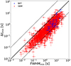 |
Fig. 1. Plot representing Δtmin versus FWHMmin for the GRBs in common. Red points show GBM data, where Δtmin was taken from G15 and V23, while blue points are BAT data, with Δtmin being taken from Golkhou & Butler (2014). Equality is shown with a solid line, while dashed lines show ±1 dex. |
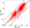 |
Fig. 2. Plot representing Δtmin versus Δtdet for the GRBs in common. Δtmin is the MVT estimate from G15 and V23 obtained with GBM, while Δtdet is the detection timescale found with MEPSA. Solid and dashed lines have the same meaning as in Figure 1. |
According to simulations carried out in Guidorzi (2015) and C23, the brighter the pulse, the smaller the ratio of Δtdet/FWHM. Specifically, C23 came up with a calibrated relation between FWHMmin and Δtdet, which they used to estimate the former from the latter while also using other ancillary information yielded by MEPSA and modelling the corresponding uncertainty (see Equation A3 therein).
Our analysis confirms that Δtmin is more closely related with the detection timescale (Figure 2) and the rise time, tr (Figure 3), than the FWHM (Figure 1) of the pulse, as also mentioned by G15. Indeed, Δtdet ∼ Δtmin ∼ tr, with median values of 0.6 and 1.1 for Δtdet/Δtmin and Δtmin/tr, respectively. The GRB pulses are typically asymmetric, with a decay-to-rise time ratio of 3–4. As a consequence, the FWHM is comparably longer than the rise time alone and explains why FWHMmin is longer than Δtmin by a comparable factor. This difference between FWHMmin and Δtmin is important to bear in mind, especially when it is to be interpreted within a theoretical context.
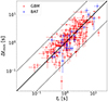 |
Fig. 3. Plot showing Δtmin versus the rise time tr of the fitted pulse for the samples of GRBs defined in Appendix A. Red points show GBM data, where Δtmin was taken from G15 and V23, while blue points are BAT data, with Δtmin taken from Golkhou & Butler (2014). The solid and dashed lines have the same meaning as in Figure 1. |
3.2. FWHMmin–T90 plane
Following C23, in Figure 4 we plot FWHMmin versus T90 for the bursts of our sample. We also computed the median value of FWHMmin for the various GRB classes and applied two-population Kolmogorov-Smirnov (KS) tests to investigate their mutual compatibility. Results are reported in Table 3. Clearly, LGRBs show greater FWHMmin values, with a median value of 2.4 s, while it is about 0.2 s for the SGRBs. The GRBs with an ascertained SN association have typical FWHMmin values similar to the bulk of LGRBs, with a median value of about 1.6 s, thus pointing towards a common collapsar origin for the bulk of LGRBs.
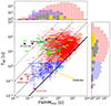 |
Fig. 4. Scatter plot of FWHMmin and T90 for the Fermi/GBM sample along with the corresponding marginal distributions. Blue (red) points represent short (long) GRBs. Gold points represent SN-associated GRBs. Magenta, lime, and cyan points represent SEE-GRBs from Lien et al. (2016), Lan et al. (2020), Kaneko et al. (2015), respectively. Three extragalactic MGFs candidates, 180128A, 200415A, and 231115A, are shown in brown. The SEE-GRBs from the three samples considered are shown altogether in grey in the top and right panel. We also show with a black star the two peculiar LGRBs, 211211A and 230307A, associated with a kilonova event and 191019A, which may be a short GRB that exploded in a dense environment. We also highlight the peculiar short collapsar GRB 200826A associated with an SN. |
Median FWHMmin values for different GRB groups along with the p-values of the two-population KS test between the FWHMmin values of each corresponding pair of groups.
Conversely, SEE-GRBs FWHMmin values (about 0.15 s) are closer to those of SGRBs than LGRBs, supporting a common origin. Our results are consistent with those of Kaneko et al. (2015) and Lan et al. (2020). Among them, 161129A was also noted by Guidorzi et al. (2024a) to have a combination of high variability V ∼ 0.6, relatively low luminosity ( , and short MVT, which is potentially characteristic of long-duration merger candidates. The initial spike has an MVT of about 20 ms, although it is slightly below the threshold detection of our technique, having
  for the 4 ms binned LC.
Long-duration merger candidates, such as 211211A and 230307A, are definite outliers in the LGRB FWHMmin distribution, with an MVT of 5 and 17 ms, respectively. These two cases show that duration alone could be misleading and showcase the potential of MVT to unveil these baffling merger candidates, as already pointed out in C23 and V23. Notably, 2% of LGRBs have FWHMmin ≤ 0.1 s, indicating that LGRBs could include unidentified merger candidates. A few of these events, which also look similar to canonical SEE-GRBs, are displayed in Figure 5. Additionally, we considered 191019A, a long GRB (T90 = 64 s) at redshift z = 0.248 and with no associated SN, which might also be a merger candidate (Levan et al. 2023; Stratta et al. 2025). We note that 191019A was not detected by GBM; however, using Swift/BAT data, Camisasca et al. (2023a) reported an MVT of 0.196 s. Assuming the scaling of FWHMmin with photon energy (see Appendix D), we estimated that we would have found 0.14−0.15 s with the GBM, placing 191019A in the outskirts of the LGRB FWHMmin distribution. 221009A is not included in this analysis, owing to the strong saturation issues in Fermi/GBM. A MVT of 0.1 s, obtained with HXMT/HE data, was reported by Zhang et al. (2025), compatible with both Type I and II FWHMmin distributions.
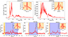 |
Fig. 5. Top panels: LC of 211211A (left) and of 230307A (right) when using the 8–1000 keV range. Bottom panels, left to right: LC of 080807, 090720B, and 090832A, respectively (in the same energy range as top panels). The yellow window includes the initial short spike, while the blue one includes the extended emission. The inset in each panel shows a zoom-in on the narrowest pulse. The black point indicates the detection timescale, Δtdet, of the narrowest pulse, while the orange region shows the window encompassing FWHMmin. |
The MGFs have a mean FWHMmin of 12 ms, hence exhibiting even shorter values than typical SGRBs. Table 3 shows the median FWHMmin value for the different populations as well as the result of the KS tests.
3.3. Peak rate versus FWHMmin
In line with the procedure of C23, we characterised the detection efficiency of MEPSA applied to GBM data as a function of both FWHMmin and PRmax, the latter being the maximum peak rate of any given pulse. To this aim, we generated synthetic pulses assuming the Norris function (Norris et al. 1996) and added a constant background with a count rate selected from a sample of real background rates observed with GBM. For each GRB, the background rate is the sum of the individual rates across all the NaI detectors involved. Poisson noise was finally simulated for the total expected counts per bin. We simulated GRBs with PRmax ranging from 102 to 105 cts s−1 and with FWHMmin going from 10−2 to 102 s. For each point of this grid, we simulated 100 pulses and estimated the detection efficiency by counting how many times MEPSA detected the peak with a S/N > 5. The detection efficiency, ϵdet, is approximately described by a linear function of the logarithm of both quantities:
 (1)
(1)
The optimal coefficients were found to be a = 1.27, b = 2.83, and c = −7.33. Eq. (1) is the GBM analogous of Eq. (2) of C23:
 (2)
(2)
The meaning of Eq. (2) is illustrated by the following example: For a pulse with MVT of 10 ms to be correctly identified with 90% confidence, its peak rate has to be ≳6430 cts s−1 (a condition that is fulfilled by just 13% of the bursts in our sample). Figure 6 illustrates ϵdet in the PRmax–FWHMmin plane.
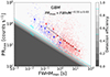 |
Fig. 6. For the GBM sample, PRmax versus FWHMmin. Blue dots represent Type-I GRBs (i.e. SGRBs and SEE-GRBs), while red dots represent Type-II GRBs. Lighter dots correspond to individual GRB data, and darker dots indicate the geometric mean of data from GRB groups sorted by increasing FWHMmin. Each Type-I group consists of 50 GRBs; each Type-II group consists of 270 GRBs. Dotted lines show the best fit for Type-II GRBs. Shaded areas illustrate ten regions with a detection efficiency ranging from 0 to 1. Cyan dashed lines indicate the 50% and 90% detection efficiency contours. |
3.4. Peak luminosity versus FWHMmin
We computed the isotropic-equivalent peak luminosities, Lp, as done in Maccary et al. (2024) for 152 collapsar-candidate GRBs with known redshift. We studied the Lp − FWHMmin correlation, which was observed in other catalogues (C23). The result is shown in Figure 7.
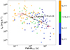 |
Fig. 7. Peak luminosity versus FWHMmin for collapsar-candidate (or Type-II) GRBs. The red points represent the geometric means of GRB groups sorted by increasing FWHMmin. The dashed line indicates the best fit. GRBs are also categorised by the number of peaks, with the more luminous ones having more peaks. |
The selection effects significantly influence the distribution in the Lp − FWHMmin plane. Specifically, narrower pulses require a higher peak rate to be detected. This selection bias could hide possible weak and short bursts that could contribute to demote the correlation. To account for this bias, we carried out a suite of simulations following the procedure set up in C23. We divided our sample into nine bins of redshift and simulated points within the Lp − FWHMmin plane for each bin. For each bin, we randomly generated as many points as in the corresponding observed sub-sample, where Lp was drawn from the distribution of the observed luminosities in that bin and FWHMmin was sampled from a probability density function derived from Gaussian kernel density estimation of the Type-II LGRBs with known redshift. Each point was accepted or rejected based on two conditions: (1) a Bernoulli trial with probability p = ϵdet calculated using Eq. (1) for that specific point was successful, and (2) the isotropic energy of this synthetic pulse did not exceed the maximum observed energy in that bin, given by  .
.
We carried out N = 104 simulations. In this way, we did not assume any correlation between Lp and FWHMmin, whereas the resulting apparent correlation is entirely due to the selection effects (Figure 8).
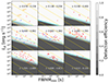 |
Fig. 8. Diagram showing Lp versus FWHMmin for the Fermi/GBM divided into nine redshift bins with equal logarithmic spacing in luminosity distance. The blue dots represent merger-candidates (or Type-I GRBs), and red dots represent collapsar-candidates (or Type-II GRBs). The dashed cyan lines show 90% and 50% detection efficiency (vertical bars). Gold dashed lines indicate regions of constant isotropic-equivalent released energy (in erg) for each peak, roughly calculated as |

We then applied Pearson, Spearman, and Kendall correlation tests to the real data using logarithmic values for the analysis. For Type-II GRBs, we obtained p-values of 8 × 10⁻¹⁵, 2.5 × 10⁻¹⁴, and 8 × 10⁻¹³, respectively. In contrast, we found no evidence of such a correlation for Type-I GRBs, with p-values of 0.96, 0.83, and 0.86, respectively. We then applied the same correlation test to the N = 104 simulated datasets to build the corresponding reference distributions for the p-values that account for the selection effects discussed above. The results are shown in Figure 9 and reveal that the simulated datasets were more correlated than the real ones only in 0.5%, 2.1%, and 2.3% of cases, respectively, which represent the probabilities that the observed correlation could arise purely from selection effects.
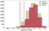 |
Fig. 9. Pearson, Spearman, and Kendall correlation p-values (in logarithm units) computed on N = 104 simulated samples (blue, olive, and red histograms) compared to the ones computed on the real dataset (blue, olive, and red dashed lines, respectively). |
3.5. Number of peaks versus FWHMmin
Figure 10 shows FWHMmin versus the number of peaks within a GRB. GRBs with numerous peaks (peak-rich GRBs) tend to have shorter MVTs compared with those with fewer peaks (peak-poor GRBs), as was also observed in Swift/BAT GRBs (Guidorzi et al. 2016). The same authors also found that peak-richness correlates with a shallower power density spectrum, which means that shorter timescales have relatively more temporal power than in peak-poor GRBs (Guidorzi et al. 2024b).
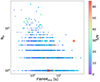 |
Fig. 10. Number of pulses within a GRB as a function of FWHMmin colour-coded by S/N. The GRBs that are composed of a large number of pulses are more likely to have a shorter FWHMmin. |
3.6. Lorentz factor versus FWHMmin
We took the Lorentz factors (LFs, hereafter noted as Γ0) from the same references as in C23, that is Lü et al. (2012), Xue et al. (2019), and Xin et al. (2016). We found 95 GRBs both detected by Fermi/GBM and reported in these studies. For 87 of them, Xue et al. (2019) made use of the Liso − Ep − Γ0 correlation to get pseudo values of Γ0, while for the remaining nine, we used the early afterglow peak to compute Γ0. We then considered additional references for individual GRBs: 140102A, whose Γ0 was reported by Gupta et al. (2021) (who also modelled the forward and reverse shock), as well as 211211A and 230307A. The value of the LF of 211211A (approximately Γ0 ∼ 1000) has been obtained by modelling the forward shock (Mei et al. 2022) and by measuring the deceleration peak (Veres et al. 2023). According to Zhong et al. (2024), 230307A has log(Γ0)∼2.77. Our sample also includes one SGRB, 090510, which is a rare case of SGRB detected by Fermi/LAT. In this case, Γ0 was estimated from the peak of the high-energy afterglow (Ghirlanda et al. 2010). The other SGRB in our sample is 170817A, for which a considerably less reliable measure of Γ0 was obtained using Ep, i − Eiso and Γ0 − Eiso correlations (Zou et al. 2018). We also considered the sample of GRBs from Ghirlanda et al. (2018) separately. We collected 65 Type-II GRBs in common with our sample, with 26 of them being part of their golden or silver sample and 39 taken as upper limits. We also report the six cases of Type-I GRBs for which a measure of Γ0 is possible. The results are shown in Figure 11. The left panel shows FWHMmin versus Γ0, while the right panel displays FWHMmin versus Γ0 as measured by Ghirlanda et al. (2018).
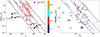 |
Fig. 11. For the Type-II (red dots) and Type-I GRBs (purple squares) present in our sample, FWHMmin versus the initial Lorentz factor Γ0. In the left panel, the Γ0 values are from different datasets and colour-coded as follows: L12 Lü et al. (2012), X19 Xue et al. (2019), X16 Xin et al. (2016), and Gu21 Gupta et al. (2021). The dashed lines represent the typical distance |
We computed the radius, R, at which the gamma-ray emission is produced using
![Mathematical equation: $$ \begin{aligned} R\ =\ 2\, c\, \Gamma _{0}^{2}\ \mathrm{FWHM}_{\rm min}\ = 6 \times 10^{14}\ \mathrm{cm}\ \Bigg [\frac{\Gamma _0}{100}\Bigg ]^{2}\Bigg [\frac{\mathrm{FWHM}_{\rm min}}{1\ \mathrm{s}}\Bigg ]. \end{aligned} $$](/articles/aa/full_html/2025/10/aa55418-25/aa55418-25-eq17.gif) (3)
(3)
Eq. (3) is derived from the IS model (Rees & Meszaros 1994; Daigne & Mochkovitch 1998). We used FWHMmin as a proxy of the MVT in the emission radius calculation rather than Δtmin because the former can be considered as the sum of the rise and the decay time, while the latter gives only the rise time. This choice was motivated by the fact that the emission radius in the IS framework is linked to the angular spreading timescale, R/cΓ2, which also governs the decay time of the pulse (Kobayashi et al. 2002). Since the decay of GRB pulses is three to four times slower than the rise, it is more accurate to consider FWHMmin than Δtmin when computing the emission radius. Figure 12 shows the R distribution for the Type-II GRBs in our sample. The emission radii, R, for all of our GRBs range from 1014 to 1017 cm. Notably, 80% of the bursts have R values greater than 1015 cm, with a mean value of ∼ 6 × 1015 cm. As a further test, we computed the deceleration radius, Rdec, and we checked that R < Rdec using
 (4)
(4)
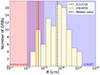 |
Fig. 12. Source emission region radii for the GBM sample. The red and orange vertical lines represent the value of this radius for 211211A and 230307A, while the dashed vertical line represents the median value of the distribution. The red shaded regions indicate the values expected by the IS model (1013 cm ≲ R ≲1015 cm; Rees & Meszaros 1994; Daigne & Mochkovitch 1998), while the blue one indicates the expectations for the ICMART model (R ≳ 1014−15 cm; Zhang & Yan (2011)). In the decade 1014 − 15 cm (purple), the two regions overlap, and the emission radii in this region are marginally compatible with both models. |
where Eiso, 52 = Eiso/1052 erg and Γ2 = Γ/100, with Eiso being the explosion energy ( , with efficiency η) and n the medium density. This was derived from Sari & Piran (1999), Molinari et al. (2007) and corresponds to the thin shell case. We assumed a constant density medium of n = 1 cm−3 and an efficiency of η = 0.2. We found only two cases where R > Rdec, namely 090423 and 171222A, with R/Rdec ratios of 1.1 and 1.3, respectively. Unfortunately, there is no broadband modelling of the afterglow for these GRBs, so we are unable to verify whether our fiducial values are accurate estimates of the explosion energy and medium density in these cases.
3.7. Peak energy versus FWHMmin
We explored the relationship between the MVT and the peak energy, Ep. We took the Ep information from the GBM catalogue (Goldstein et al. 2012). For 1921 bursts, measures of both Ep and FWHMmin are available. For a subsample of 107 with measured redshift, we could also compute the rest-frame peak energy Ep, i = (1 + z) Ep. We calculated the Pearson, Spearman, and Kendall correlation coefficients using the logarithmic values, which turned out to be −0.29, −0.30, and −0.21, with associated p-values of (5, 2.4, and 2)×10−4, respectively. This suggests that the two quantities are somehow correlated, despite the large dispersion, as shown in Figure 13.
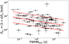 |
Fig. 13. For all Type-II GRBs with known redshift, Ep, i versus FWHMmin. The solid red line shows the best fit, while the two dashed red lines show the dispersion of the correlation. |
We fitted the data with a power law, log(Ep/keV) = m log(FWHMmin/s) + q, and modelled the dispersion as a further parameter, minimising the D’Agostini likelihood (D’Agostini 2005). This likelihood is suitable to model correlations affected by a significant scatter, which is treated as a model parameter and is referred to as intrinsic dispersion of the correlation, denoted with σ. The resulting parameters are  , q = 2.66 ± 0.07, and
  .
.
4. Discussion and conclusions
As previously investigated in C23, we confirm that FWHMmin is a robust estimate of the MVT, although it carries a slightly different meaning compared to G15, which is more tightly connected to the rise time of the pulse. The MEPSA detection timescale, however, also proves to be a good indicator of the rise time of the narrowest pulse, thus providing a very simple and practical method to compute it. These differences are important to keep in mind, especially when the MVT values are interpreted within a theoretical context.
In the IS model, the hydrodynamic timescale and the angular spreading timescale govern the rise and the decay time of a GRB pulse, respectively (e.g. Kobayashi et al. 2002). The hydrodynamic timescale, which dictates the rise time, is the shock-crossing time, approximately ∼l/c, where l represents the characteristic irregularity scale or shell width in the outflow. The angular spreading timescale, which determines the decay time, results from the time delay or spread due to the angular extent of the emission region. This timescale is roughly R/cΓ2, where R is the emission radius and Γ is the Lorentz factor of the emission region. Since most observed pulses exhibit a faster rise than decay, the pulse width is primarily set by the angular spreading time.
We confirm that millisecond-long pulses are very rare in GRBs. While partly affected by detection thresholds, their scarcity appears to be a genuine feature. Having investigated three independent studies, we confirm that SEE-GRBs have shorter MVTs than LGRBs, compatible with the bulk of SGRBs. Additionally, the three well-known long-duration merger candidates 211211A, 230307A, and 191019A to a lesser extent have very short MVTs (5, 17, and 150 ms), providing further evidence that short MVTs are characteristic of Type-I GRBs, regardless of the total duration. Our MVT results align with the conventional interpretation that SEE-GRBs are essentially SGRBs with an additional emission component. The exact physical mechanism behind the extended emission remains unclear. Several models have been proposed, including long-lasting activity from the central engine, such as a magnetar formed during the merger (Metzger et al. 2008; Jordana-Mitjans et al. 2022) or energy release from a late fallback accretion disc (Rosswog 2007; Musolino et al. 2024), both of which can continue powering the emission after the main burst. These results emphasise the importance of multi-wavelength follow-up observations, particularly for LGRBs with low MVTs, as these could reveal other merger events that might otherwise be misclassified as collapsar candidates.
The differences in MVT between Type-I and Type-II GRBs may indicate distinct progenitors or disparities in jet propagation. The irregularity in GRB jets arises from a combination of internal factors, such as variability in the central engine, and external factors such as interaction with the surrounding medium and jet instabilities. The conventional central engines are magnetars or black hole accretion disc systems. Even if both types of GRBs are powered by black hole accretion discs, the black holes in Type I events (SGRBs) likely have smaller masses, resulting in shorter dynamical timescales. The GRB jets must also penetrate a dense medium surrounding the central engines: a stellar envelope in the case of LGRBs (Type II) or neutron star merger ejecta in the case of SGRBs (Type I). This interaction fosters the growth of hydrodynamic instabilities along the jet boundary (e.g. Gottlieb et al. 2020). Type II jets are likely more unstable due to the higher density of the surrounding stellar envelope. Additionally, pulses emitted within the photospheric radius are obscured, adding further complexity. Extragalactic MGFs have an even shorter MVT than every GRB population, thus offering an additional tool to distinguish them from traditional GRB events.
We have confirmed, using an independent dataset, that in the case of Type-II GRBs, peak luminosity does correlate with FWHMmin, while the same does not hold true for Type-I GRBs. The question as to whether this is a result of a much poorer sample or due to the intrinsic absence of correlation will be addressed through future richer datasets. We confirmed that GRBs with many pulses (pulse-rich GRBs, as defined in Guidorzi et al. 2024b) tend to have shorter MVTs, supporting the presence of two temporal behaviours: rapid variability atop a slower FRED-like envelope and purely slow, FRED-like evolution. This distinction may reflect differences in central engine activity, circumburst interactions, or progenitor type. We computed the LF and source emission radius, R. The R values we found generally do not align with the IS model, where R typically ranges from 1013 to 1014 cm. However, they are consistent with the ICMART model, which predicts gamma-ray emission at larger radii, R > 1015−16 cm (Zhang & Yan 2011), through magnetic reconnection cascades.
We have investigated the plausible correlation between MVT and peak energy. Given the established anti-correlation between MVT and peak luminosity (see also C23, Wu et al. 2016) and the known correlation between peak energy and peak luminosity (Yonetoku et al. 2004; Ghirlanda et al. 2005), in principle, we expected an anti-correlation between the MVT and Ep, i. Moreover, several GRBs with a small MVT have also been detected at higher energies by Fermi/LAT, such as 080916C (0.3 s, Tajima et al. 2008); 090510 (0.011 s, Ohno & Pelassa 2009); 090720B (0.014 s, Rubtsov et al. 2012); and 210410A (0.07 s, Arimoto et al. 2021). Although we do find a correlation, it is very dispersed. Smaller MVTs may imply shorter angular spreading times and smaller emission radii, resulting in higher shock energy density in the emission region. In the standard synchrotron shock model, a constant fraction of the shock energy is transferred to magnetic fields, with radiation from smaller radii generally expected to be harder. However, since both the shock energy generated through internal dissipation and the blue-shift of emission frequencies depend on the Lorentz factor, velocity irregularities in the outflow–an essential assumption of the IS model–can introduce significant dispersion in this relationship.
Data availability
Table 1 is available at the CDS via https://cdsarc.cds.unistra.fr/viz-bin/cat/J/A+A/702/A95.
Acknowledgments
We are grateful to the anonymous reviewer for their precious report which helped us to cross-check our results and to overall improve the quality of this work. R.M. and M.M. acknowledge the University of Ferrara for the financial support of their PhD scholarships. L.F. acknowledges support from the AHEAD-2020 Project grant agreement 871158 of the European Union’s Horizon 2020 Program. A.T. acknowledges financial support from ASI-INAF Accordo Attuativo HERMES Pathfinder operazioni n. 2022-25-HH.0 and the basic funding program of the Ioffe Institute FFUG-2024-0002. L.A. acknowledges support from INAF Mini-grant programme 2022. A.E.C received support from the European Research Council (ERC) via the ERC Synergy Grant ECOGAL (grant 855130). Views and opinions expressed by ERC-funded scientists are however those of the author(s) only and do not necessarily reflect those of the European Union or the European Research Council. Neither the European Union nor the granting authority can be held responsible for them. M. B. acknowledges the Department of Physics and Earth Science of the University of Ferrara for the financial support through the FIRD 2024 grant.
References
- Abbott, B. P., Abbott, R., Abbott, T. D., et al. 2017, ApJ, 848, L13 [CrossRef] [Google Scholar]
- Ackermann, M., Ajello, M., Asano, K., et al. 2014, Science, 343, 42 [NASA ADS] [CrossRef] [Google Scholar]
- Arimoto, M., Ohno, M., Longo, F., Axelsson, M., & Fermi-LAT Team 2021, GRB Coordinates Network, 29781, 1 [Google Scholar]
- Bhat, P. N., Briggs, M. S., Connaughton, V., et al. 2012, ApJ, 744, 141 [NASA ADS] [CrossRef] [Google Scholar]
- Blinnikov, S. I., Novikov, I. D., Perevodchikova, T. V., & Polnarev, A. G. 1984, Sov. Astron. Lett., 10, 177 [Google Scholar]
- Bulla, M., Camisasca, A. E., Guidorzi, C., et al. 2023, GRB Coordinates Network, 33578, 1 [Google Scholar]
- Burns, E., Svinkin, D., Hurley, K., et al. 2021, ApJ, 907, L28 [NASA ADS] [CrossRef] [Google Scholar]
- Camisasca, A. E., Guidorzi, C., Amati, L., et al. 2023a, A&A, 671, A112 [NASA ADS] [CrossRef] [EDP Sciences] [Google Scholar]
- Camisasca, A. E., Guidorzi, C., Bulla, M., et al. 2023b, GRB Coordinates Network, 33577, 1 [NASA ADS] [Google Scholar]
- Chen, J.-M., Zhu, K.-R., Peng, Z.-Y., & Zhang, L. 2024, MNRAS, 527, 4272 [Google Scholar]
- D’Agostini, G. 2005, ArXiv e-prints [arXiv: physics/0511182] [Google Scholar]
- Dai, C.-Y., Guo, C.-L., Zhang, H.-M., Liu, R.-Y., & Wang, X.-Y. 2024, ApJ, 962, L37 [Google Scholar]
- Daigne, F., & Mochkovitch, R. 1998, MNRAS, 296, 275 [NASA ADS] [CrossRef] [Google Scholar]
- Della Valle, M., Chincarini, G., Panagia, N., et al. 2006, Nature, 444, 1050 [NASA ADS] [CrossRef] [Google Scholar]
- Di Matteo, T., Perna, R., & Narayan, R. 2002, ApJ, 579, 706 [Google Scholar]
- Dimple, Misra, K., & Arun, K. G. 2023, ApJ, 949, L22 [Google Scholar]
- Dimple, Misra, K., & Arun, K. G. 2024, ApJ, 974, 55 [Google Scholar]
- Du, Z., Lü, H., Yuan, Y., Yang, X., & Liang, E. 2024, ApJ, 962, L27 [Google Scholar]
- Eichler, D., Livio, M., Piran, T., & Schramm, D. N. 1989, Nature, 340, 126 [NASA ADS] [CrossRef] [Google Scholar]
- Fenimore, E. E., in ’t Zand, J. J. M., Norris, J. P., Bonnell, J. T., & Nemiroff, R. 1989, ApJ, 448, L101 [Google Scholar]
- Dalessi, S., Roberts, O. J., Meegan, C., & Fermi GBM Team 2023, GRB Coordinates Network, 33411, 1 [Google Scholar]
- Fermi-Lat Collaboration 2021, Nat. Astron., 5, 385 [CrossRef] [Google Scholar]
- Feroci, M., Frontera, F., Costa, E., et al. 1999, ApJ, 515, L9 [Google Scholar]
- Fruchter, A. S., Levan, A. J., Strolger, L., et al. 2006, Nature, 441, 463 [NASA ADS] [CrossRef] [Google Scholar]
- Fynbo, J. P. U., Watson, D., Thöne, C. C., et al. 2006, Nature, 444, 1047 [NASA ADS] [CrossRef] [Google Scholar]
- Galama, T. J., Vreeswijk, P. M., van Paradijs, J., et al. 1998, Nature, 395, 670 [Google Scholar]
- Garcia-Cifuentes, K., Becerra, R. L., De Colle, F., Cabrera, J. I., & Del Burgo, C. 2023, ApJ, 951, 4 [Google Scholar]
- Gehrels, N., Norris, J. P., Barthelmy, S. D., et al. 2006, Nature, 444, 1044 [NASA ADS] [CrossRef] [Google Scholar]
- Ghirlanda, G., Ghisellini, G., & Firmani, C. 2005, MNRAS, 361, L10 [NASA ADS] [Google Scholar]
- Ghirlanda, G., Ghisellini, G., & Nava, L. 2010, A&A, 510, L7 [NASA ADS] [CrossRef] [EDP Sciences] [Google Scholar]
- Ghirlanda, G., Nappo, F., Ghisellini, G., et al. 2018, A&A, 609, A112 [NASA ADS] [CrossRef] [EDP Sciences] [Google Scholar]
- Goldstein, A., Preece, R. D., & Briggs, M. S. 2010, ApJ, 721, 1329 [Google Scholar]
- Goldstein, A., Burgess, J. M., Preece, R. D., et al. 2012, ApJS, 199, 19 [Google Scholar]
- Goldstein, A., Cleveland, W. H., & Kocevski, D. 2022, Fermi GBM Data Tools: v1.1.1 [Google Scholar]
- Golkhou, V. Z., & Butler, N. R. 2014, ApJ, 787, 90 [NASA ADS] [CrossRef] [Google Scholar]
- Golkhou, V. Z., Butler, N. R., & Littlejohns, O. M. 2015, ApJ, 811, 93 [NASA ADS] [CrossRef] [Google Scholar]
- Gompertz, B. P., Ravasio, M. E., Nicholl, M., et al. 2023, Nat. Astron., 7, 67 [Google Scholar]
- Gottlieb, O., Bromberg, O., Singh, C. B., & Nakar, E. 2020, MNRAS, 498, 3320 [NASA ADS] [CrossRef] [Google Scholar]
- Guidorzi, C. 2015, Astron. Comput., 10, 54 [NASA ADS] [CrossRef] [Google Scholar]
- Guidorzi, C., Dichiara, S., & Amati, L. 2016, A&A, 589, A98 [NASA ADS] [CrossRef] [EDP Sciences] [Google Scholar]
- Guidorzi, C., Maccary, R., Tsvetkova, A., et al. 2024a, A&A, 690, A261 [NASA ADS] [CrossRef] [EDP Sciences] [Google Scholar]
- Guidorzi, C., Sartori, M., Maccary, R., et al. 2024b, A&A, 685, A34 [NASA ADS] [CrossRef] [EDP Sciences] [Google Scholar]
- Gupta, R., Oates, S. R., Pandey, S. B., et al. 2021, MNRAS, 505, 4086 [NASA ADS] [Google Scholar]
- Hjorth, J., Sollerman, J., Møller, P., et al. 2003, Nature, 423, 847 [Google Scholar]
- Hurley, K., Cline, T., Mazets, E., et al. 1999, Nature, 397, 41 [NASA ADS] [CrossRef] [Google Scholar]
- Hurley, K., Boggs, S. E., Smith, D. M., et al. 2005, Nature, 434, 1098 [NASA ADS] [CrossRef] [Google Scholar]
- Janiuk, A., Yuan, Y., Perna, R., & Di Matteo, T. 2007, ApJ, 664, 1011 [NASA ADS] [CrossRef] [Google Scholar]
- Jespersen, C. K., Severin, J. B., Steinhardt, C. L., et al. 2020, ApJ, 896, L20 [NASA ADS] [CrossRef] [Google Scholar]
- Jin, Z.-P., Li, X., Cano, Z., et al. 2015, ApJ, 811, L22 [NASA ADS] [CrossRef] [Google Scholar]
- Jordana-Mitjans, N., Mundell, C. G., Guidorzi, C., et al. 2022, ApJ, 939, 106 [NASA ADS] [CrossRef] [Google Scholar]
- Kaneko, Y., Bostancı, Z. F., Göğüş, E., & Lin, L. 2015, MNRAS, 452, 824 [NASA ADS] [CrossRef] [Google Scholar]
- Kobayashi, S., Piran, T., & Sari, R. 1997, ApJ, 490, 92 [Google Scholar]
- Kobayashi, S., Ryde, F., & MacFadyen, A. 2002, ApJ, 577, 302 [NASA ADS] [CrossRef] [Google Scholar]
- Kumar, P., & Narayan, R. 2009, MNRAS, 395, 472 [NASA ADS] [CrossRef] [Google Scholar]
- Lan, L., Lu, R.-J., Lü, H.-J., et al. 2020, MNRAS, 492, 3622 [NASA ADS] [CrossRef] [Google Scholar]
- Lei, W.-H., Zhang, B., & Liang, E.-W. 2013, ApJ, 765, 125 [Google Scholar]
- Lesage, S., Veres, P., Briggs, M. S., et al. 2023, ApJ, 952, L42 [NASA ADS] [CrossRef] [Google Scholar]
- Levan, A. J., Malesani, D. B., Gompertz, B. P., et al. 2023, Nat. Astron., 7, 976 [NASA ADS] [CrossRef] [Google Scholar]
- Levan, A. J., Gompertz, B. P., Salafia, O. S., et al. 2024, Nature, 626, 737 [NASA ADS] [CrossRef] [Google Scholar]
- Lien, A., Sakamoto, T., Barthelmy, S. D., et al. 2016, ApJ, 829, 7 [Google Scholar]
- Lü, H.-J., Liang, E.-W., Zhang, B.-B., & Zhang, B. 2010, ApJ, 725, 1965 [Google Scholar]
- Lü, J., Zou, Y.-C., Lei, W.-H., et al. 2012, ApJ, 751, 49 [CrossRef] [Google Scholar]
- Lü, H.-J., Zhang, B., Liang, E.-W., Zhang, B.-B., & Sakamoto, T. 2014, MNRAS, 442, 1922 [Google Scholar]
- Lyutikov, M., Pariev, V. I., & Blandford, R. D. 2003, ApJ, 597, 998 [Google Scholar]
- Maccary, R., Guidorzi, C., Amati, L., et al. 2024, ApJ, 965, 72 [NASA ADS] [CrossRef] [Google Scholar]
- MacFadyen, A. I., & Woosley, S. E. 1999, ApJ, 524, 262 [NASA ADS] [CrossRef] [Google Scholar]
- MacLachlan, G. A., Shenoy, A., Sonbas, E., et al. 2013, MNRAS, 432, 857 [NASA ADS] [CrossRef] [Google Scholar]
- Mazets, E. P., Golentskii, S. V., Ilinskii, V. N., Aptekar, R. L., & Guryan, I. A. 1979, Nature, 282, 587 [NASA ADS] [CrossRef] [Google Scholar]
- Mazets, E. P., Aptekar, R. L., Cline, T. L., et al. 2008, ApJ, 680, 545 [Google Scholar]
- Meegan, C., Lichti, G., Bhat, P. N., et al. 2009, ApJ, 702, 791 [Google Scholar]
- Mei, A., Banerjee, B., Oganesyan, G., et al. 2022, Nature, 612, 236 [NASA ADS] [CrossRef] [Google Scholar]
- Mereghetti, S., Rigoselli, M., Salvaterra, R., et al. 2024, Nature, 629, 58 [NASA ADS] [CrossRef] [Google Scholar]
- Metzger, B. D., Quataert, E., & Thompson, T. A. 2008, MNRAS, 385, 1455 [CrossRef] [Google Scholar]
- Metzger, B. D., Giannios, D., Thompson, T. A., Bucciantini, N., & Quataert, E. 2011, MNRAS, 413, 2031 [Google Scholar]
- Minaev, P. Y., Pozanenko, A. S., Grebenev, S. A., et al. 2024, Astron. Lett., 50, 1 [Google Scholar]
- Molinari, E., Vergani, S. D., Malesani, D., et al. 2007, A&A, 469, L13 [NASA ADS] [CrossRef] [EDP Sciences] [Google Scholar]
- Musolino, C., Duqué, R., & Rezzolla, L. 2024, ApJ, 966, L31 [NASA ADS] [CrossRef] [Google Scholar]
- Narayan, R., Paczynski, B., & Piran, T. 1992, ApJ, 395, L83 [NASA ADS] [CrossRef] [Google Scholar]
- Norris, J. P., & Bonnell, J. T. 2006, ApJ, 643, 266 [NASA ADS] [CrossRef] [Google Scholar]
- Norris, J. P., Nemiroff, R. J., Bonnell, J. T., et al. 1996, ApJ, 459, 393 [NASA ADS] [CrossRef] [Google Scholar]
- Norris, J. P., Bonnell, J. T., Kazanas, D., et al. 2005, ApJ, 627, 324 [NASA ADS] [CrossRef] [Google Scholar]
- Ofek, E. O., Kulkarni, S. R., Nakar, E., et al. 2006, ApJ, 652, 507 [Google Scholar]
- Ohno, M., & Pelassa, V. 2009, GRB Coordinates Network, 9334, 1 [Google Scholar]
- Paczynski, B. 1986, ApJ, 308, L43 [NASA ADS] [CrossRef] [Google Scholar]
- Paczynski, B. 1991, Acta Astron., 41, 257 [NASA ADS] [Google Scholar]
- Paczyński, B. 1998, ApJ, 494, L45 [Google Scholar]
- Planck Collaboration VI. 2020, A&A, 641, A6 [NASA ADS] [CrossRef] [EDP Sciences] [Google Scholar]
- Popham, R., Woosley, S. E., & Fryer, C. 1999, ApJ, 518, 356 [NASA ADS] [CrossRef] [Google Scholar]
- Rastinejad, J. C., Gompertz, B. P., Levan, A. J., et al. 2022, Nature, 612, 223 [NASA ADS] [CrossRef] [Google Scholar]
- Rees, M. J., & Meszaros, P. 1994, ApJ, 430, L93 [Google Scholar]
- Roberts, O. J., Veres, P., Baring, M. G., et al. 2021, Nature, 589, 207 [NASA ADS] [CrossRef] [Google Scholar]
- Rodi, J. C., Pacholski, D. P., Mereghetti, S., et al. 2025, ApJ, 979, L25 [Google Scholar]
- Rosswog, S. 2007, MNRAS, 376, L48 [NASA ADS] [Google Scholar]
- Rubtsov, G. I., Pshirkov, M. S., & Tinyakov, P. G. 2012, MNRAS, 421, L14 [NASA ADS] [Google Scholar]
- Salmon, L., Hanlon, L., & Martin-Carrillo, A. 2022, Galaxies, 10, 78 [Google Scholar]
- Sari, R., & Piran, T. 1999, ApJ, 520, 641 [NASA ADS] [CrossRef] [Google Scholar]
- Scargle, J. D., Norris, J. P., Jackson, B., & Chiang, J. 2013, ApJ, 764, 167 [Google Scholar]
- Steinhardt, C. L., Mann, W. J., Rusakov, V., & Jespersen, C. K. 2023, ApJ, 945, 67 [Google Scholar]
- Stratta, G., Nicuesa Guelbenzu, A. M., Klose, S., et al. 2025, ApJ, 979, 159 [Google Scholar]
- Svinkin, D., Frederiks, D., Hurley, K., et al. 2021, Nature, 589, 211 [NASA ADS] [CrossRef] [Google Scholar]
- Tajima, H., Bregeon, J., Chiang, J., & Thayer, G. 2008, GRB Coordinates Network, 8246, 1 [Google Scholar]
- Thompson, T. A., Chang, P., & Quataert, E. 2004, ApJ, 611, 380 [NASA ADS] [CrossRef] [Google Scholar]
- Trigg, A. C., Burns, E., Roberts, O. J., et al. 2024, A&A, 687, A173 [NASA ADS] [CrossRef] [EDP Sciences] [Google Scholar]
- Troja, E., Fryer, C. L., O’Connor, B., et al. 2022, Nature, 612, 228 [NASA ADS] [CrossRef] [Google Scholar]
- Tsvetkova, A., Amati, L., Bulla, M., et al. 2025, A&A, 698, A169 [NASA ADS] [CrossRef] [EDP Sciences] [Google Scholar]
- Usov, V. V. 1992, Nature, 357, 472 [NASA ADS] [CrossRef] [Google Scholar]
- Veres, P., Bhat, P. N., Burns, E., et al. 2023, ApJ, 954, L5 [NASA ADS] [CrossRef] [Google Scholar]
- Vianello, G., Gill, R., Granot, J., et al. 2018, ApJ, 864, 163 [NASA ADS] [CrossRef] [Google Scholar]
- Wheeler, J. C., Yi, I., Höflich, P., & Wang, L. 2000, ApJ, 537, 810 [NASA ADS] [CrossRef] [Google Scholar]
- Woosley, S. E. 1993, ApJ, 405, 273 [Google Scholar]
- Wu, Q., Zhang, B., Lei, W.-H., et al. 2016, MNRAS, 455, L1 [NASA ADS] [CrossRef] [Google Scholar]
- Xiao, S., Peng, W.-X., Zhang, S.-N., et al. 2022, ApJ, 941, 166 [Google Scholar]
- Xin, L.-P., Wang, Y.-Z., Lin, T.-T., et al. 2016, ApJ, 817, 152 [NASA ADS] [CrossRef] [Google Scholar]
- Xiong, S., Wang, C., & Huang, Y. Gecam Team 2023, GRB Coordinates Network, 33406, 1 [Google Scholar]
- Xue, L., Zhang, F.-W., & Zhu, S.-Y. 2019, ApJ, 876, 77 [NASA ADS] [CrossRef] [Google Scholar]
- Yang, B., Jin, Z.-P., Li, X., et al. 2015, Nat. Commun., 6, 7323 [NASA ADS] [CrossRef] [Google Scholar]
- Yang, J., Chand, V., Zhang, B.-B., et al. 2020, ApJ, 899, 106 [NASA ADS] [CrossRef] [Google Scholar]
- Yang, J., Ai, S., Zhang, B. B., et al. 2022, Nature, 612, 232 [NASA ADS] [CrossRef] [Google Scholar]
- Yang, Y.-H., Troja, E., O’Connor, B., et al. 2024, Nature, 626, 742 [NASA ADS] [CrossRef] [Google Scholar]
- Yonetoku, D., Murakami, T., Nakamura, T., et al. 2004, ApJ, 609, 935 [Google Scholar]
- Yoon, S. C., & Langer, N. 2005, A&A, 443, 643 [NASA ADS] [CrossRef] [EDP Sciences] [Google Scholar]
- Zhang, B. 2006, Nature, 444, 1010 [NASA ADS] [CrossRef] [Google Scholar]
- Zhang, B., & Yan, H. 2011, ApJ, 726, 90 [Google Scholar]
- Zhang, W.-L., Xue, W.-C., Li, C.-K., et al. 2025, ApJ, 986, 170 [Google Scholar]
- Zhong, S.-Q., Li, L., Xiao, D., et al. 2024, ApJ, 963, L26 [Google Scholar]
- Zhu, S.-Y., Sun, W.-P., Ma, D.-L., & Zhang, F.-W. 2024, MNRAS, 532, 1434 [Google Scholar]
- Zou, Y.-C., Wang, F.-F., Moharana, R., et al. 2018, ApJ, 852, L1 [Google Scholar]
S/N ≥ 7, 6.8, 6.4, 6 at 1, 4, 64, 1024 ms.
We used the function bayesian_blocks from the astropy.stats python library.
Appendix A: FWHMmin compared to a direct fit of the narrowest pulse
We compared FWHMmin measurements obtained using MEPSA calibration and the procedure described in C23 with the results derived from fitting the LC with FRED shaped pulses (denoted as FWHMfit; see Maccary et al. (2024) for a detailed description of the technique). To do so, we analysed a sub-sample of GRBs with either one or a few peaks, for which a direct and accurate modelling of the pulses’ shapes and FWHMs was feasible. We initially selected 639 single-peaked GRBs with S/N > 10. We excluded the GRBs that displayed a more complex temporal structure than a single well-shaped pulse, ending up with 544 GRBs. Their pulses were then fitted with a FRED template and discarded the cases, whose best-fit parameters were too close to the boundaries (chosen to avoid unrealistic parameter values), or with relative errors on the rise time greater than 50%, reducing the sample to 410 GRBs. We used Swift/BAT data as well, taking a sub-sample of GRBs with less than 8 peaks in their LC. After intersecting these data with the G15 and V23 results, we retained 244 GRBs in the GBM sample and 28 in the BAT sample for a comparative analysis. In Fig. A.1 we illustrated the comparison between FWHMmin and FWHMfit, showing how closely the two methods agree across different GRBs. As we can see, for most peaks,  ; more precisely, 90% of events are in the range
  .
.
We furthermore performed a linear fit of the form y = mx + q, applied to the logarithmic values, modelling the intrinsic dispersion σint as a further parameter, adopting the D’Agostini likelihood (D’Agostini 2005). Optimising the parameters using MCMC, we found  ,
,  , and
, and  . The uncertainty on log FWHMmin, previously estimated as σmin = 0.13 (i.e a 35% relative error on FWHMmin), leads to a total uncertainty, accounting for the intrinsic dispersion σint, of
  (41%). This implies that the relative error made when using FWHMmin instead of FWHMfit is approximately 41%, as opposed to the 35% estimated on synthetic LCs by Camisasca et al. (2023a). This comparison ensures the robustness of our MVT measurements by validating them against an established LC fitting method.
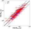 |
Fig. A.1. Plot presenting FWHMmin computed either by following the method described in C23, or by directly fitting the narrowest pulse by a Norris function (called here FWHMfit). Red (blue) points were obtained using GBM (resp. BAT) data. The black line indicates the equality line while the dashed lines show a factor 2 of discrepancy, illustrating that most measurements fall within this range. |
Appendix B: Comparison between BAT and GBM
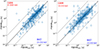 |
Fig. B.1. Left: FWHMmin computed by C23 with BAT data on 15-150 keV against the FWHMmin of the same bursts but computed in this work on GBM data on the 8-1000 keV range. Right: Same but the GBM energy range is restricted to 15-150 keV to be the same as BAT. |
We compared the results obtained by C23 with BAT data with those obtained in this work with GBM data. The FWHMmin obtained with the GBM is in mean twice as small as those obtained with the BAT. This was expected due to the dependance of the MVT on the energy band. We also carried this analysis restricting the GBM energy range to the Swift/BAT one (15-150 keV). The results show a dispersion around the equality line but no general trend, indicating that our results are consistent with the ones of C23. The results of these two analyses are shown in Figure B.1.
Appendix C: FWHMmin compared with Bayesian blocks
In this section, we compared our results with those obtained by segmenting the LC using Bayesian blocks4 (BBs, Scargle et al. 2013). We applied BBs, using a false alarm threshold of p0 = 10−3 to a sample of 96 GRBs, chosen with FWHMmin < 50 ms. This choice was made to obtain enough GRBs to make a sound statistical analysis and to include bright GRBs with evident sub-second structures with exquisite S/N. This sample includes, for instance, GRBs as 211211A, 230307A, 190114C, and others known for their rapid temporal variability and brightness, making them ideal test cases. We computed the MVT using BBs, defining it as the shortest block in the segmentation, ΔTBB. Figure C.1 compares these values with those from the MEPSA-based approach. The points scatter around the equality line without a clear systematic bias in either direction. The distribution of the ratio ΔTBB/FWHMmin is shown in Fig. C.2 with a median of about 1.03–meaning that, on average, BBs yield MVT values ∼3% larger than those obtained with MEPSA. The 90 % confidence interval is [0.4-2.3], meaning that for most GRBs, the discrepancy between the MVTs obtained using BBs and those obtained using MEPSA is smaller than a factor of 2. We further estimated that in roughly 60% cases, the temporal structures identified by MEPSA and BBs coincide; in such cases the discrepancies in MVT values arise only from different ways of estimating the width. BBs, which approximate the pulse as a rectangle, tend to overestimate the width, whereas MEPSA uses a more realistic, though simplified, pulse shape.
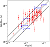 |
Fig. C.1. Plot of FWHMmin versus the shortest segment of the BBs segmentation, ΔTBB. Blue points represents the GRBs shown in Fig. 5. |
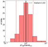 |
Fig. C.2. Distribution of the ratio ΔTBB over FWHMmin. The solid black line represents the case FWHMmin = ΔTBB, while the dashed one shows the median value. The two red dashed lines enclose the 90 % confidence interval [0.4-2.3]. |
Appendix D: Dependence of FWHMmin on energy
We computed FWHMmin as a function of the geometric mean of the energy range boundaries, for six different energy ranges: 8-30, 8-90, 30-90, 8-1000, 90-300, and 90-1000 keV. We carried out this analysis on 286 bursts, each having a measured FWHMmin with S/N > 7 across all six energy ranges. We found that FWHMmin ∝ E−α with αmean = 0.46 ± 0.19, with a standard dispersion of σ = 0.7, and αmedian = 0.26 ± 0.12. Results are shown in Figure D.1. The results are consistent with those of C23 that obtained αmean = 0.45 ± 0.08, αmedian = 0.54 ± 0.07 and those of Fenimore et al. (1989): α ∈ [0.37; 0.46].
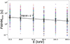 |
Fig. D.1. Plot showing FWHMmin as a function of the geometric mean of the energy range boundaries. The coloured dots are the FWHMmin of 286 bursts in four different energy ranges: 8-30, 8-90, 30-90, 8-1000, 90-300, and 90-1000 keV. The values on the x-axis are the geometric means of the corresponding energy boundaries. Black dots with error bars are the weighted averages of the FWHMmin for each energy range and the black dashed line is the power-law that best fit the black points. |
All Tables
Median FWHMmin values for different GRB groups along with the p-values of the two-population KS test between the FWHMmin values of each corresponding pair of groups.
All Figures
|
Fig. 1. Plot representing Δtmin versus FWHMmin for the GRBs in common. Red points show GBM data, where Δtmin was taken from G15 and V23, while blue points are BAT data, with Δtmin being taken from Golkhou & Butler (2014). Equality is shown with a solid line, while dashed lines show ±1 dex. |
| In the text | |
|
Fig. 2. Plot representing Δtmin versus Δtdet for the GRBs in common. Δtmin is the MVT estimate from G15 and V23 obtained with GBM, while Δtdet is the detection timescale found with MEPSA. Solid and dashed lines have the same meaning as in Figure 1. |
| In the text | |
|
Fig. 3. Plot showing Δtmin versus the rise time tr of the fitted pulse for the samples of GRBs defined in Appendix A. Red points show GBM data, where Δtmin was taken from G15 and V23, while blue points are BAT data, with Δtmin taken from Golkhou & Butler (2014). The solid and dashed lines have the same meaning as in Figure 1. |
| In the text | |
|
Fig. 4. Scatter plot of FWHMmin and T90 for the Fermi/GBM sample along with the corresponding marginal distributions. Blue (red) points represent short (long) GRBs. Gold points represent SN-associated GRBs. Magenta, lime, and cyan points represent SEE-GRBs from Lien et al. (2016), Lan et al. (2020), Kaneko et al. (2015), respectively. Three extragalactic MGFs candidates, 180128A, 200415A, and 231115A, are shown in brown. The SEE-GRBs from the three samples considered are shown altogether in grey in the top and right panel. We also show with a black star the two peculiar LGRBs, 211211A and 230307A, associated with a kilonova event and 191019A, which may be a short GRB that exploded in a dense environment. We also highlight the peculiar short collapsar GRB 200826A associated with an SN. |
| In the text | |
|
Fig. 5. Top panels: LC of 211211A (left) and of 230307A (right) when using the 8–1000 keV range. Bottom panels, left to right: LC of 080807, 090720B, and 090832A, respectively (in the same energy range as top panels). The yellow window includes the initial short spike, while the blue one includes the extended emission. The inset in each panel shows a zoom-in on the narrowest pulse. The black point indicates the detection timescale, Δtdet, of the narrowest pulse, while the orange region shows the window encompassing FWHMmin. |
| In the text | |
|
Fig. 6. For the GBM sample, PRmax versus FWHMmin. Blue dots represent Type-I GRBs (i.e. SGRBs and SEE-GRBs), while red dots represent Type-II GRBs. Lighter dots correspond to individual GRB data, and darker dots indicate the geometric mean of data from GRB groups sorted by increasing FWHMmin. Each Type-I group consists of 50 GRBs; each Type-II group consists of 270 GRBs. Dotted lines show the best fit for Type-II GRBs. Shaded areas illustrate ten regions with a detection efficiency ranging from 0 to 1. Cyan dashed lines indicate the 50% and 90% detection efficiency contours. |
| In the text | |
|
Fig. 7. Peak luminosity versus FWHMmin for collapsar-candidate (or Type-II) GRBs. The red points represent the geometric means of GRB groups sorted by increasing FWHMmin. The dashed line indicates the best fit. GRBs are also categorised by the number of peaks, with the more luminous ones having more peaks. |
| In the text | |
|
Fig. 8. Diagram showing Lp versus FWHMmin for the Fermi/GBM divided into nine redshift bins with equal logarithmic spacing in luminosity distance. The blue dots represent merger-candidates (or Type-I GRBs), and red dots represent collapsar-candidates (or Type-II GRBs). The dashed cyan lines show 90% and 50% detection efficiency (vertical bars). Gold dashed lines indicate regions of constant isotropic-equivalent released energy (in erg) for each peak, roughly calculated as |
| In the text | |
|
Fig. 9. Pearson, Spearman, and Kendall correlation p-values (in logarithm units) computed on N = 104 simulated samples (blue, olive, and red histograms) compared to the ones computed on the real dataset (blue, olive, and red dashed lines, respectively). |
| In the text | |
|
Fig. 10. Number of pulses within a GRB as a function of FWHMmin colour-coded by S/N. The GRBs that are composed of a large number of pulses are more likely to have a shorter FWHMmin. |
| In the text | |
|
Fig. 11. For the Type-II (red dots) and Type-I GRBs (purple squares) present in our sample, FWHMmin versus the initial Lorentz factor Γ0. In the left panel, the Γ0 values are from different datasets and colour-coded as follows: L12 Lü et al. (2012), X19 Xue et al. (2019), X16 Xin et al. (2016), and Gu21 Gupta et al. (2021). The dashed lines represent the typical distance |
| In the text | |
|
Fig. 12. Source emission region radii for the GBM sample. The red and orange vertical lines represent the value of this radius for 211211A and 230307A, while the dashed vertical line represents the median value of the distribution. The red shaded regions indicate the values expected by the IS model (1013 cm ≲ R ≲1015 cm; Rees & Meszaros 1994; Daigne & Mochkovitch 1998), while the blue one indicates the expectations for the ICMART model (R ≳ 1014−15 cm; Zhang & Yan (2011)). In the decade 1014 − 15 cm (purple), the two regions overlap, and the emission radii in this region are marginally compatible with both models. |
| In the text | |
|
Fig. 13. For all Type-II GRBs with known redshift, Ep, i versus FWHMmin. The solid red line shows the best fit, while the two dashed red lines show the dispersion of the correlation. |
| In the text | |
|
Fig. A.1. Plot presenting FWHMmin computed either by following the method described in C23, or by directly fitting the narrowest pulse by a Norris function (called here FWHMfit). Red (blue) points were obtained using GBM (resp. BAT) data. The black line indicates the equality line while the dashed lines show a factor 2 of discrepancy, illustrating that most measurements fall within this range. |
| In the text | |
|
Fig. B.1. Left: FWHMmin computed by C23 with BAT data on 15-150 keV against the FWHMmin of the same bursts but computed in this work on GBM data on the 8-1000 keV range. Right: Same but the GBM energy range is restricted to 15-150 keV to be the same as BAT. |
| In the text | |
|
Fig. C.1. Plot of FWHMmin versus the shortest segment of the BBs segmentation, ΔTBB. Blue points represents the GRBs shown in Fig. 5. |
| In the text | |
|
Fig. C.2. Distribution of the ratio ΔTBB over FWHMmin. The solid black line represents the case FWHMmin = ΔTBB, while the dashed one shows the median value. The two red dashed lines enclose the 90 % confidence interval [0.4-2.3]. |
| In the text | |
|
Fig. D.1. Plot showing FWHMmin as a function of the geometric mean of the energy range boundaries. The coloured dots are the FWHMmin of 286 bursts in four different energy ranges: 8-30, 8-90, 30-90, 8-1000, 90-300, and 90-1000 keV. The values on the x-axis are the geometric means of the corresponding energy boundaries. Black dots with error bars are the weighted averages of the FWHMmin for each energy range and the black dashed line is the power-law that best fit the black points. |
| In the text | |
Current usage metrics show cumulative count of Article Views (full-text article views including HTML views, PDF and ePub downloads, according to the available data) and Abstracts Views on Vision4Press platform.
Data correspond to usage on the plateform after 2015. The current usage metrics is available 48-96 hours after online publication and is updated daily on week days.
Initial download of the metrics may take a while.