| Issue |
A&A
Volume 702, October 2025
|
|
|---|---|---|
| Article Number | A135 | |
| Number of page(s) | 24 | |
| Section | The Sun and the Heliosphere | |
| DOI | https://doi.org/10.1051/0004-6361/202555609 | |
| Published online | 24 October 2025 | |
Solar wind temperature measurements
1
Christian Albrechts University at Kiel, Kiel, Germany
2
Institut de Recherche en Astrophysique et Planétologie, Toulouse Cedex 4, France
⋆ Corresponding author: This email address is being protected from spambots. You need JavaScript enabled to view it.
Received:
21
May
2025
Accepted:
6
August
2025
Abstract
Context. The solar wind has been an active research area since the beginning of the space age and the available measurements of its basic properties, i.e. solar wind density, velocity, and temperature, have fundamentally shaped our understanding of the heliosphere. Meanwhile, the data from various solar wind instruments show significant systematic differences.
Aims. We characterise systematic errors in these basic solar wind properties that are caused by instrumental limitations and put them in the context of solar wind studies.
Methods. To this end, we investigated the limitations that arise from the finite resolution of state-of-the-art solar wind instruments, namely the Proton Alpha Sensor (PAS) and the Solar Probe ANalyzer for Ions (SPAN-I). We defined two models, a virtual detector model of PAS and a more general further idealised detector with finite resolution. Virtual measurements of Maxwell-Boltzmann velocity distribution functions were compared to observations. The detailed effects of the instrumental resolution on the solar wind density, velocity, and temperature were analysed.
Results. We identify an unphysical direction dependence of the observed temperatures in data from PAS and SPAN-I. We show that both models can reproduce and explain this apparent direction dependence of the temperature observed by PAS. While the solar wind densities and the absolute values of the solar wind velocity are well determined, the directions of the solar wind velocity suffer from systematic errors and more importantly the majority of all available solar wind temperatures are systematically overestimated to varying degrees. These systematic errors are a compulsory consequence of the finite resolution of an instrument and are further enhanced by the detailed instrumental responses. In addition, limited instrumental sensitivity and field of view lead to a systematic and variable underestimation of the temperature. All observed temperatures are affected by one or more of these effects. Our results are transferable to all solar wind instruments.
Conclusions. Our results have far-reaching consequences for heliophysics. Firstly, we provide guidelines to adapt requirements for future solar wind instruments. These guidelines stem from our finding that the resolution of existing solar wind instruments is insufficient to capture all relevant underlying physics. Secondly, we discuss the impact of our results for past and future studies in various aspects of heliophysics. Even long-standing fundamental findings need to be reconsidered in the light of our results.
Key words: plasmas / instrumentation: detectors / solar wind
© The Authors 2025
 Open Access article, published by EDP Sciences, under the terms of the Creative Commons Attribution License (https://creativecommons.org/licenses/by/4.0), which permits unrestricted use, distribution, and reproduction in any medium, provided the original work is properly cited.
This article is published in open access under the Subscribe to Open model. This email address is being protected from spambots. You need JavaScript enabled to view it. to support open access publication.
1. Introduction
Since the beginning of the space age in 1957, measurements of the solar wind have been used in countless studies. These studies have revolutionised our understanding in numerous topics, reaching from the large-scale structure of our heliosphere, through medium-scale structures such as corotating interaction regions and coronal mass ejections, down to the very small scale of local wave-particle interaction in an unique almost collisionless plasma. But although much scientific progress has been achieved, many detailed processes of the generation and the evolution of the solar wind are not yet well understood. To shed light on these open questions, the focus of the scientific community has moved to study shorter timescales and smaller spatial scales Marsch (2006). For example, already with Helios, different temperatures had been observed parallel and perpendicular to the magnetic field direction (Marsch et al. 1982). Such temperature anisotropies are interpreted as the result of wave-particle interactions (Marsch 2006) and are expected to drive plasma instabilities (Yoon 2017), and various theoretical and simulation studies offer possible explanations (e.g. Lazar et al. 2022). The common fundamentals for these research topics are accurately observed temperatures that provide the same accuracy for all directions and all bulk solar wind velocities.
However, there is ample evidence that observations of solar wind properties by different instruments show systematic differences beyond the individually calculated uncertainties. Often a cross-correlation approach is used to characterise the differences or to even cross-calibrate datasets (e.g. King & Papitashvili 2005; Ipavich et al. 1998). While a comparison can be insightful, cross-calibration of instruments ignores and obfuscates the root cause of the systematic differences. Further, it relies on various assumptions; for example, that one of the instruments reflects the ground truth. Moreover, the influence of the instrumental resolution on the fundamental solar wind parameters, i.e. solar wind bulk density, velocity, and temperature, to our knowledge have not yet been conclusively investigated. Very recently in an independent concurrent study, Nicolaou et al. (2025) investigated the difficulties of recovering particle Velocity Distribution Function (VDF)s due to the limited energy resolution and limited angular resolution for a virtual detector. Our study combines a data-driven investigation with a theoretical perspective on the measurement of solar wind properties. In fact, measuring solar wind with sufficient accuracy is a challenging task. Solar wind instruments have to cover bulk flow energies that are in the kilo-electronvolt range. Simultaneously, thermal energies that are in the electronvolt range have to be resolved. While the technological progress over the decades is mainly reflected in the better time resolution of solar wind instruments, the energy and angular resolution has remained similar (see Table 1 in Podesta 2015). Podesta (2015) investigated the influence of small non-thermal features on obtained solar wind bulk velocities. They find that the resolution of existing solar wind instruments is about one order of magnitude too low to resolve such features, which leads to uncertainties in the determined bulk velocities.
Here, we analyse the influence of the instrumental resolution on the solar wind bulk density, velocity, and temperature under the assumption of thermal velocity distributions. We find that the provided instrumental resolution, which is often just given by (i) the grid spacing of the instruments bins or (ii) a simple estimation of the broadness of the response function in a given channel, is in fact insufficient to describe the actual resolution of solar wind instruments. For an accurate evaluation of the instrumental resolution, it is necessary to utilise the detailed 3D response function of an instrument to characterise the resolution dependent on different velocity distribution functions. Even if the velocity distribution function is known, such detailed analyses cannot provide a fixed resolution but rather a range of systematic errors of the measurements.
Furthermore, here we restrict ourselves to thermal velocity distributions, that are the easiest use case that should be reliably resolved by solar wind instruments. Any systematic limitations that occur for thermal velocity distributions are even more problematic for all studies focusing on non-thermal features; for example, temperature anisotropies. Section 2 describes the relation between solar wind velocity distributions and the solar wind bulk properties that are commonly used to characterise the solar wind. A general overview of what is actually measured by solar wind instruments is given in Section 3. In this study, we chose two solar wind instruments, the Proton Alpha Sensor (PAS) and the Solar Probe ANalyzer for Ions (SPAN-I), as test cases. They are part of two of the latest solar missions, Solar Orbiter (SolO) run by the European Space Agency (ESA), and Parker Solar Probe (PSP) run by the National Aeronautics and Space Administration (NASA). We compare their observations with theoretical predictions based on their respective instrumental resolutions. Both instruments are described in Section 3.1. Solar wind temperatures recorded by both instruments show evidence of insufficient instrumental resolution, shown in Section 3.2. In Section 4, a Virtual Detector based on PAS (VPAS) is presented. This VPAS is used to analyse artificial thermal velocity distributions and the results are compared with PAS data. Theoretical limits on the accuracy of measured temperatures are derived in Section 5, based on a further idealised instrument. These limits are compared to the results of Section 4.2. Differences between data from PAS and SPAN-I that have been taken under similar conditions are discussed with respect to their different instrumental resolutions in Section 6. All findings are summarised and conclusions for the design of future solar wind instruments and for past and future studies that build on the available solar wind measurements are drawn in Section 7.
2. Solar wind velocity distributions and bulk properties
Routinely the bulk solar wind is characterised by three properties: the proton density, velocity, and temperature. Depending on the capabilities of the different sensors, velocity and temperature are provided in one, two, or three dimensions. Independent of the instrument, none of the three parameters can be measured directly. Rather, the phase space distribution of protons is sampled and the parameters are derived from these distributions. The phase space distribution, δn(r, mv, t), is 7D, wherein r, and mv are the coordinates in position and momentum space, respectively, and t is the time. For non-relativistic solar wind protons, velocity space can be used instead of momentum space. In the following, we use Cartesian coordinates and indices x,y,z denote the three directions in position, and velocity space, respectively.
For in situ measurements the position, r, naturally is given by the position of the instrument (i.e. the spacecraft position). The resolutions in v and t depend on the capabilities of the instrument.
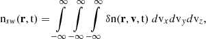
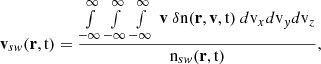
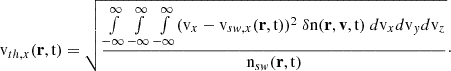
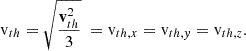
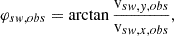
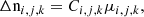
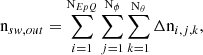
The position r and time t, dependent density, nsw, bulk flow speed, vsw, and thermal velocity, vth, can be calculated as the 0th, 1st, and 2nd order moments of the distribution in velocity space,
 (1)
(1)
 (2)
(2)
 (3)
(3)
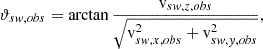
The y and z components of vth(r, t) are defined analogously to Eq. (3). Often the thermal velocity is used to describe the temperature of the solar wind, but also temperatures in Kelvin and electronvolt are widely used. These relate to the thermal velocity as
![Mathematical equation: $$ \begin{aligned} {\mathrm{T} }_{x}&= \frac{{\mathrm{m} }}{k_{B}} \mathbf v _{th,x}^2\ [\mathrm{K} ]\end{aligned} $$](/articles/aa/full_html/2025/10/aa55609-25/aa55609-25-eq4.gif) (4)
(4)
![Mathematical equation: $$ \begin{aligned} k_{B}{\mathrm{T} }_{x}&= \frac{{\mathrm{m} }}{e} \mathbf v _{th,x}^2\ [\mathrm{eV} ], \end{aligned} $$](/articles/aa/full_html/2025/10/aa55609-25/aa55609-25-eq5.gif) (5)
(5)
with mass, m, elementary charge, e, and Boltzmann constant, kB, and as for Eq. (3) the y and z components of the vector T are not shown here. The conversion from electronvolt to Kelvin is given by e/kB or 1 eV ≈ 11 605 K. From now on, we adopt the same notation as used in the PAS and SPAN-I datasets and refer to the kinetic temperature in electronvolt also simply as T instead of kBT. Also note that throughout this study all temperatures and thermal velocities are solar wind properties, but for the sake of readability we omit the subindex, sw, for temperatures and thermal velocities but not for the density and bulk velocity.
The moments are well defined and make no a priori assumptions about the nature of the underlying distributions. But in turn they do not provide any information on the shape of the underlying distributions. This information is lost and the interpretation of each moment as the most likely respective value is only valid for symmetric distributions. The meaning of the 1st and 2nd moments is ambiguous. The most commonly used alternative to moments is a fit of an a priori-defined model VDF to the observed VDF. This fit approach is also affected by the instrumental resolution and in addition requires strongly limiting assumptions in the form of the model VDF. In practice, observed VDFs are often interpolated (e.g. De Marco et al. 2023). However, the interpolation introduces additional assumptions and resulting uncertainties. For instance, even for the same model VDF the determined solar wind properties can differ depending on the degree of a polynomial interpolation. Further, if the response functions of neighbouring bins overlap, as is the case, for example, for PAS and SPAN-I (as is discussed in the following sections), a meaningful interpolation is even more difficult to define. Thus, although our considerations are also relevant for other approaches, in the following we focus on solar wind properties derived as moments of the VDF.
Often the most fundamental assumption of a thermalised distribution is made. In this case, the derived moments can be used to describe the distribution at place r and time t by a Maxwell-Boltzmann distribution,
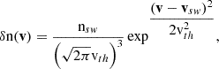 (6)
(6)
with the scalar property,
 (7)
(7)
However, often non-thermal features are observed. One typical non-thermal feature is a beam that is aligned with the local magnetic field direction. A second non-thermal feature is a temperature anisotropy with respect to the local magnetic field direction. To study these, an additional measurement of the local magnetic field, B, is required, and the measured distributions have to be transformed into a magnetic field aligned frame first.
Table A.1 provides an overview on the meaning of the various super- and sub-indices used in the following sections. In particular, Table A.1 summarises under which conditions redundant indices are omitted.
3. Solar wind measurements
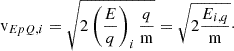
Although the detailed design and measurement technique of solar wind instruments varies, there is one common feature that is shared by most (if not all) of them. Incoming particles are filtered by their ratio of energy-per-charge (EpQ), by means of electrostatic deflection. For an ion species with mass, m, and a charge, q, each given EpQ step, (E/q)i, i ∈ {1, …, NEpQ}, corresponds to a unique energy, q (E/q)i = Ei, q. Thus, an electrostatic analyser implements a velocity filter:
 (8)
(8)
Stepping through i ∈ {1, …, NEpQ} yields 1D velocity spectra. Many instruments allow one to further discriminate one or two inflow directions, and thereby yield 2D or 3D velocity spectra. The individual sensors differ most in their respective methods to discriminate the inflow directions. On three axes stabilised spacecraft typically ion optics are used to determine directionality. On spinning spacecraft a mechanical collimator can be utilised to determine the direction perpendicular to the spin axis.
While some instruments utilise other designs such as Faraday cups (e.g. Case et al. 2020; Bosqued et al. 1996; Bridge et al. 1977), here we focus on the most commonly used so called top-hat design (e.g. Schwenn et al. 1975; Bame et al. 1992; McFadden et al. 2008; Reme et al. 1997; Owen et al. 2020; Livi et al. 2022; Galvin et al. 2008). However, our approach also holds for all designs utilising electrostatic analysers and in principle also for all instruments with a finite resolution. Top-hat electrostatic analysers are composed of two stacked spherical segment shaped plates with slightly different curvature radii. In addition to the EpQ stepping as described above, this design allows one to measure the azimuthal direction. Due to the ion optical properties of the top hat design, the position of the ion at the exit of the electrostatic analyser can be used to determine the incoming azimuthal angle, ϕ, in the plane of the detector for Nϕ values of ϕ. A second electrostatic deflection can be used to determine Nθ values of the elevation angle, θ, perpendicular to this plane. With electrostatic analyser and deflection voltages that are stepped through, the instant Field of View (FoV) covers only a small part of the full velocity space. Thereby, it takes a total scan time, tscan, to scan velocity space at NEpQ ⋅ Nϕ ⋅ Nθ points (vx, vy, vz)i, j, k wherein i, j, k denote a combination of an instrumental EpQ step, an azimuthal angle bin, and an elevation angle bin. As an example of an instrumental velocity space coverage, Fig. 1 illustrates the 2D velocity space coverage of PAS for its central elevation step. The black dots mark the central position of instrumental bins, (vx, vy, vz)i, j, k, which are scanned by the instrument. The instrument integrates the velocity space density around these central positions from a certain volume with a response, δℛi, j, k(v, φ, ϑ). The boxes around each centre illustrate an idealised situation where the volumes of adjacent bins do not overlap, i.e. within the FoV the complete velocity space is uniquely covered. For this case the resulting uncertainty can be expressed by the finite grid spacing of the bin centres, we call this uncertainty ΔGS. But there is also a second measure for the uncertainty in v, the width of δℛi, j, k(v, φ, ϑ), which is often given as Full Width Half Maximum (FWHM). We call this uncertainty due to the response width, ΔRW. In the literature, both ΔGS and ΔRW or a mix of both are referred to as instrumental resolution. Often it is not clear which of both is actually used. In Fig. 1 only ΔGSv is illustrated, ΔRWv is addressed beginning in Sect. 4.
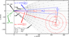 |
Fig. 1. Example of a 2D cut of a velocity phase-space scan is shown. The black dots mark the central position of instrumental bins (vx, i, j, k, vy, i, j, k) that are scanned, with i ∈ [1, …, NEpQ], j ∈ [1, …, Nϕ], NEQP as the number of energy-per-charge (EpQ) steps and Nϕ as the number of azimuthal bins, the angle of inflow bin ϕj of the jth azimuthal bin, and its corresponding bin width ΔGSϕj. As an example for a solar wind instrument the calibration values of the central elevation bin k = 5 of PAS for protons are used here and in Fig. 3. Note that we explicitly differentiate between the instrumental properties (ϕ, θ), and the measured angles (φsw, obs and ϑsw, obs). All instrumental characteristics are shown in black including the utilised Frame of Reference (FoR). Dots illustrate the shells centred at the origin, i.e. in the Spacecraft Reference Frame (SRF), which are scanned by the electrostatic analyser. Each 5th electrostatic analyser step is enlarged for clarity. The shape of each instrumental bin is illustrated with a concentric grid. The instrumental resolution in velocity space becomes coarser with increasing shell radius. In red, an example of a thermalised Maxwell-Boltzmann VDF (see Eq. (6)) is depicted. Shown are the bulk-flow vector relative to the instrument vsw, its components, vsw, x, vsw, y, and the thermal velocity vth. The corresponding 1σ, 2σ, and 3σ environments of the distribution are indicated in light red. In blue, measurement quantities are shown: the absolute value of the solar wind bulk velocity |vsw|, the y component of the thermal speed vth, y, and the corresponding thermal angle αy. The two relevant FoRs are depicted in the left part of the figure: the SRF in black and the Radial-Tangential-Normal Frame (RTN) frame in green. Therein, the tangential components points in the direction of the spacecraft eigenvelocity. |
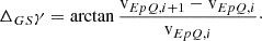
In the radial direction, the uncertainty ΔGSvi is defined by the spacing of (E/q)i. By design the uncertainty ΔRW(E/q)i is proportional to (E/q)i, and thus in the radial direction the uncertainty ΔRWvi is proportional to vEpQ, i. To obtain a wide and continuous phase space coverage the (E/q)i are typically spaced logarithmically. This means that both ΔRWv and ΔGSv in radial direction of velocity space become coarser with increasing vEpQ. This scaling behaviour transfers also to the velocity resolutions in the φ and ϑ directions, as the angular grid spacings ΔGSϕ and ΔGSθ do not depend on vEpQ1. Fig. 1 also illustrates how a thermalised Maxwell-Boltzman VDF would be seen by such an instrument. The angular width under which the distribution is seen by the instrument scales not only with the thermal velocity vth but also with vsw. As a measure for the angular width of a VDF in the Spacecraft Reference Frame (SRF) we define the angle, α,
 (9)
(9)
as the angle under which the full 1σ-environment of the VDF would be seen by the instrument. The angle α can be directly compared with the angular resolution of instruments. Such an angle can be calculated in all three Cartesian directions. We call these angles αx, αy, αz, respectively. Fig. 1 provides an example for the angle in the y direction, αy. We emphasise that this angle is here only calculated in SRF and only to investigate effects of the instrumental resolution. Fig. B.1 illustrates how α depends on temperature and solar wind velocity.
Similarly to the y and z directions, which are expressed with the angles φ and ϑ, the radial direction can also be expressed on an angular scale. With respect to vEpQ, i, we define the angle, γ,
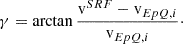 (10)
(10)
In analogy to the angular resolutions, in Table 1 and in the following sections the resolution in EpQ, (E/q)i + 1/(E/q)i, is also expressed as an angle, ΔGSγ, in velocity space, that is defined as
 (11)
(11)
γ provides a useful instrumental scale for the velocities in the x direction relative to vEpQ, i and αx can be directly compared to ΔGSγ.
Instrumental properties and resolutions of PAS, and SPAN-I, respectively.
3.1. Instruments: PAS and SPAN-I
We chose two solar wind instruments as examples: PAS, which is part of the Solar Wind Analyser (SWA) on SolO, and SPAN-I, which is part of Solar Wind Electrons Alphas and Protons (SWEAP) suite on PSP. Both utilise a top-hat design, as is described in Section 3. The details of the sensors are described in Owen et al. (2020) and Livi et al. (2022).
The two instruments have differences in their design that are relevant to consider. PAS moments can be affected by an alpha contamination, while SPAN-I has an additional time-of-flight section that allows one to distinguish directly between protons and alphas. Although the FoV of SPAN-I is wider than that of PAS, SPAN-I’s position behind PSP’s heat-shield frequently leads to incomplete coverage of the VDF in the y direction (φ direction). For PAS, L2 moment-data is available through the Solar Orbiter archive ESAC (2020) and for SPAN-I, L3 moment-data is provided via Kasper et al. (2020).
According to the metainformation provided along with the moments2, instrumental capabilities are summarised in Table 13. As the data cadence does not reflect the integration times directly, the scan times, tscan, in Table 1 are given by the times needed to complete a single phase space scan according to the instrument papers (Owen et al. 2020; Livi et al. 2022). The velocity space resolution ΔGSv in all directions of both sensors is comparable to similar solar wind instruments (see e.g. Podesta 2015), but both have an outstanding temporal resolution: A (full) scan is completed in less than one second compared to typical durations of 40–120 seconds (Schwenn et al. 1975; Bame et al. 1992; McComas et al. 1998; Galvin et al. 2008).
Both datasets allow one to investigate the effects of the instrumental resolution in the SRF according to Fig. 1, i.e. in a Frame of Reference (FoR) with the instrument at the origin. As outlined in Sect. 3, the instrumental velocity space coverage is best described by equatorial spherical coordinates, vEpQ, ϕ, θ, but moments are given in Cartesian coordinates. According to Fig. 1, we converted the observed first moments, i.e. the observed velocity vectors, vsw, obs, into absolute values, vsw, obs,
 (12)
(12)
observed azimuthal inflow angles, φsw, obs,
 (13)
(13)
and observed elevation inflow angles, ϑsw, obs,
 (14)
(14)
with Eqs. (5) and (9). Kinetic temperatures Tx, obs, Ty, obs, Tz, obs provided in electronvolt were converted to angles
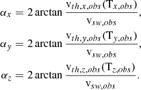 (15)
(15)
These coordinates are directly comparable to the actual velocity space scan of the instrument as illustrated in Fig. 1. For small angles, φsw, obs, ϑsw, obs, the respective resolutions, ΔGSγ, ΔGSϕ, ΔGSθ, determine the effective resolution in Cartesian x, y, z directions.
3.2. Observations: PAS and SPAN-I
In this section, we show observations from two instruments, PAS and SPAN-I, in two different directions ( and
and  , respectively) as an example. Panels b) and e) of Fig. 2 present 2D histograms of observed
  versus observed
  and observed
  versus observed
  in the instrumental frame for measured solar wind speeds 345 km/s < vsw < 355 km/s. The right hand axis transforms T to α using Eqs. (5) and (9). An arc-like structure with the base of the arches directly related to the centres of the instrumental angular bins that are marked by solid black vertical lines is clearly visible in both histograms. The dashed black lines mark the positions in the middle between two angular bins and their height is determined by the grid spacing of two adjacent bins ΔGSϕPAS and ΔGSθSPAN − I, respectively. For each arc, both position and height of the top of the arcs match the central position between two bins and the angular width of the respective instrumental bin, respectively. The distributions of observed flow angles shown in panels c) and f) peak at small absolute values; that is, close to the radial direction where the instrumental resolution in ϕ and θ direction governs the resolution in the y and z directions, respectively (compare Fig. 1). The 1D histograms of the observed temperatures shown in panels a) and d) peak at thermal angles close to the distance between instrumental bins, which is basically the instrumental resolution ΔGSϕPAS and ΔGSθSPAN − I, respectively.
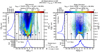 |
Fig. 2. Observed temperatures over the observed inflow direction for observed solar wind speeds between 345 and 355 km/s for 7 July 2020–30 November 2023 for PAS and for 20 April 2021–27 July 2023 for SPAN-I. Panel b): 2D histogram of PAS azimuthal temperatures |


The size and shape of these arc-like structures in PAS and SPAN-I temperatures are clearly related to the respective instrumental resolution. The direction-dependent lower bound on the observed temperatures represented by the arc-like structures is not expected for a physical process in the solar wind. If such a structure were physical, we would expect it to be independent of the direction in the SRF and to be the same in different instruments and not to adapt itself to the respective instrumental resolution. In the following section we present a virtual detector of PAS, to further investigate the influence of the instrumental resolution on derived solar wind moments.
4. Calibration-accurate virtual detector based on PAS
To understand the influence of the full instrumental response function on the derived solar wind parameters we designed a Virtual Detector based on PAS (VPAS). In this section, we put a special focus on the temperatures that are as the 2nd moment particularly sensitive to the measurement uncertainties. The VPAS is based on general considerations that are outlined in Appendix C and incorporates the most detailed 3D calibration of the PAS flight spare model that is available. VPAS is idealised in the sense that we assume that the 3D calibration perfectly and completely describes the instrumental responses4. The calibration describes the response functions, δℛi, j, k(E/q, φ, ϑ)5, for ions with energy, E, and charge, q, in spherical coordinates (compare Eq. (C.3)),
 (16)
(16)
𝒜j, k(φ, ϑ) is an area that only depends on the direction multiplied with the measurement time. ℰj, k((E/q)/(E/q)i) scales the area to an effective area along the radial axis (see also Appendix C).
Fig. 3 gives an example of the calibration data for a selection of angular bins. In panel c) the 2D angular responses for nine central bins are shown, panels b) and d) show the corresponding 1D angular responses. The 1D energy response, which is the same for all (E/q)i, is shown in panel f). In analogy to panels b) and d) the 1D angular response for successive (E/q)i are shown in panel g), where the abscissa shows the angles γ with respect to the ith EpQ step. VPAS numerically integrates the product of a given artificial input VDF and the full 3D response functions for each instrumental bin i, j, k, which result in expectation values for the number of counts, μi, j, k, in each bin, according to Eq. (C.5). These artificial measurements can be evaluated in the same way as the data from the real PAS instrument and moments can be calculated in exactly the same manner. Moments were derived from the artificial measurement by the following procedure. First, for each instrumental bin the expected counts, μi, j, k, were converted to partial densities following Eq. (C.2)
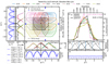 |
Fig. 3. Part of the full 3D instrumental response of PAS and VPAS. Panel c) shows the response functions of nine angular bins in the centre of the PAS FoV as contour lines. The respective indices are specified in the legend at the top of the figure. Panels b), and d), give reduced 1D response functions for the same bins. Panel f) completes the 3D instrumental response with the energy response relative to the ith (E/q)i step. The blue arrows in panel c) indicate the cut along which the VPAS input angles were scanned for panels a) and e). Panel g) give relative 1D energy responses for neighbouring steps i − 2, i − 1, i, i + 1, i + 2. For VPAS the normalised differential energy responses are interpolated. Panels a), e), and h) show the angles αz, αy, and αx, respectively, over the input angles ϑsw, in, φsw, in, and γsw, in, with solid lines and over the output angles ϑsw, out, φsw, out, and γsw, out with dashed lines. The output angles are derived based on the virtual measurement, whereas the input angles refer to the properties of the simulated solar wind distribution that is measured by VPAS. The dash-dotted lines indicate the respective input angle. Black arrows mark one maximum and one minimum in panels a) and e) and connect to the corresponding 1D response functions in panels b) and d). The shaded grey area in panel c) indicates the scan range used in Fig. 5. |
 (17)
(17)
with conversion factors, 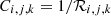 . With these discrete Δni, j, k and the bin centre velocities, vi, j, k, moments were derived by summation to obtain the output density, nsw, out:
 (18)
(18)
the output bulk speed, vsw, out:
 (19)
(19)
and the output thermal speed, vth, out, with the x component (and analogous y, z components):
 (20)
(20)
with the number of energy bins, NEpQ, the number of azimuth bins, Nϕ, and the number of elevation bins, Nθ. These derived moments can be directly compared to the moments of the input distributions. Such a comparison is discussed in detail in Sects. 4.1 and 4.2.
VPAS differs from PAS in so far as the response function  is exactly known and the total bin responses
  are derived from them (Eq. (C.4)). For any real instrument, the response can only be determined up to a certain precision, which introduces additional systematic errors. Thus, the forward (artificial measurement) and the backward (inversion of measurement back to differential densities) steps in VPAS are done under idealised conditions.
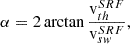
In addition, our scenario differs from the real PAS measurements in so far that the input VDF is known. For this study we exclusively investigate the simple case of thermal VDFs (see, Eq. 6). The input VDFs are therefore fully characterised by nsw, in, vsw, in, and vth, in, i.e. their first three moments. We evaluated the input VDF only in a 5σ environment centred around the bulk flow velocity. Because we used expectation values for the artificial measurements and the inversion instead of discrete counts, additional effects that arise from the limited instrumental sensitivity and statistical uncertainties are not reflected in VPAS. The parameter nsw, in of the input VDF can be chosen arbitrarily. As is outlined in Sect. 3 the instrumental angular resolutions ΔGSγ, ΔGSϕ, and ΔGSθ do not depend on vsw, in. Thus, the other input parameters, i.e. vth, in and the direction of vsw, in, can be represented with the angle αin = 2arctan(vth, in/vsw, in) and the flow directions γsw, in6, φsw, in, and ϑsw, in. Analogously to the input parameters, the output parameters vsw, out, and vth, out can be expressed by the angles αx, out, αy, out, and αz, out and γsw, out, φsw, out, and ϑsw, out.
In summary, our approach allows us to investigate the influence of the instrumental resolution under idealised conditions:
-
The VPAS measures with exactly the calibration that is used to invert the measurement of VPAS. Note that for PAS and generally for all instruments the calibration approximates the real instrumental properties.
-
By taking expectation values instead of discrete counts no statistical uncertainty is considered, especially nsw, in can be chosen arbitrarily. We therein assume an instrument with a good enough instrumental sensitivity to observe the VDF over a full 5σ environment.
-
The input thermal VDFs are well known, and are fully defined by the inflow directions γsw, in, φsw, in, ϑsw, in, and instead of vth, in we use the angle αin. Because all the angles and the instrumental grid-spacing in all directions scale with (E/q)i, a fixed reference velocity vEpQ, i can be chosen arbitrarily, i.e. the results in this section are valid for all solar wind velocities within the FoV.
As is indicated in Table A.1, in the following we omit redundant indices, i.e. the FoR which is always SRF in Sects. 4 and 5.
Results for simulated VDFs with input angles αin = αx, in = αy, in = αz, in = 1° coming in from different directions are shown in panels h), e), and a) of Fig. 3. Shown are the resulting output angles αx, out, αy, out, αz, out in the x, y, z directions over the inflow angles in γsw, in, φsw, in, and ϑsw, in direction. In each case, the respective other two angles were set to 0°. Dashed lines show αx, out, αy, out, and αz, out over the respective input directions, γsw, in, φsw, in, and ϑsw, in, and solid lines over the direction derived from the output of VPAS, γsw, out, φsw, out, and ϑsw, out, respectively. For each direction, the angles αx, out, αy, out, and αz, out do not match the respective input αin values, as the input angle is chosen smaller than the instrumental resolution in this scenario (dash-dotted lines).
For φsw, in and ϑsw, in, very small αy, out and αz, out are derived for inflow directions where only one instrumental bin has a response (see black arrows connecting the base of the arcs with the respective response for the inflow direction in Fig. 3). The highest αy, out, αz, out are observed for directions where the instrumental response is similar for two neighbouring bins (see black arrows connecting the top of the arcs with the respective response for the inflow direction in Fig. 3). Also, the resulting output flow directions are pushed towards the instrumental bin centres (compare solid and dashed blue lines). These arc-like structures in the φsw, in and ϑsw, in directions, which are also seen in the data (compare Fig. 2), are a striking feature that is highly unlikely to be a natural phenomenon in the solar wind. In the following, we argue that this feature can be explained with the 1D responses in the corresponding directions. As can be seen in Figs. 3b) and d), around the bin centres only a single bin has a non-zero response. If we imagine a very narrow, beam-like VDF with a very small temperature and if this beam-like VDF comes from an inflow direction close to a bin centre (see black arrows connecting the base of the arc to the respective instrumental response in Fig. 3), only a single instrumental bin can detect particles from this VDF. As a result a kinetic temperature of 0 eV would be derived. If a similar beam-like VDF is detected exactly between two bin centres, i.e. at the top of an arc, both bins have a similar response. As a result, a high kinetic temperature would be derived for such a cold, beam-like VDF. This situation corresponds to the top of the arc-like structures in Figs. 3a) and e). Thus, for VDFs with temperatures smaller than the grid spacing of the instrument, a derived temperature is ill-defined.
In contrast to the other two directions, for γsw, in, the αx, out are more or less constant independently from the inflow direction. This effect is a result of the strongly overlapping response functions shown in panel g) of Fig. 3. Here, at each position, three instrumental bins have a non-zero response to incoming particles. The resulting values for the first moment, in this case the absolute value of the bulk velocity, are very close to the input values (dashed and solid lines are on top of each other in panel h)), but the 2nd moment, that is the angles αx, out, are systematically overestimated. For example, a delta beam results in αx, out = 2.09°, which corresponds to a temperature Tx ≈ 1 eV (see Fig. B.1) for vsw = 500 km/s (see Fig. B.1).
As is illustrated with the example angle αin = 1° in Fig. 3, VPAS is not able to resolve such angles, i.e. temperatures, which are below the instrumental resolution ΔGSγ, ΔGSϕ, and ΔGSθ, respectively. In the following subsections, we generalise this example to a range of values for αin.
4.1. VPAS and PAS data
We now apply the virtual detector VPAS to investigate the influence of the full instrumental response function on the resulting αy, out for input angles −45° < φsw, in < 25°, at γsw, in = ϑsw, in = 0° systematically and compare the results with measurements. Analogously to Fig. 2, Fig. 4 shows a 2D histogram of the observed angle αy, obs over the observed inflow φsw, obs angle based on PAS data. Note again, all quantities are shown in SRF and not Radial-Tangential-Normal Frame (RTN) since the transformation to RTN obscures but not removes the effects discussed here and α is only meaningfully defined in SRF. Utilising αy instead of the temperature, measurements at all solar wind speeds can be directly compared. Analogously to panel e) of Fig. 3 the coloured solid lines in Fig. 4 show αout over φsw, out for VPAS, while the corresponding αin are marked with dashed coloured lines. There are two major effects to be seen:
 |
Fig. 4. Two-dimensional histogram of observed angles, αy, obs, observed by PAS from 7 July 2020 to 30 November 2023 over the determined inflow direction, φsw, obs (valid data with a quality factor of 0 only). Each column of the 2D histogram in panel b) is normalised to its respective maximum. The bins have a fixed size of 0.1° ×0.1°. 1D histograms of the observed angles, αy, out, (Panel a) and the determined inflow directions. φsw, out, (Panel c) are based on the same bin size, respectively. In addition, panel b) includes results from VPAS. For input angles αin ∈ {1, 3, 5, 7, 9, 11, 13, 15, 17, 19}° (horizontal dashed lines), the resulting output angles αy, out are given with solid lines in the same colour. 99.89% of all Ntotal = 15 476 959 valid data with a quality factor of 0 are shown here, the remaining 0.11% have αy, obs > 20°. |
Firstly, for small αy, in the same arc-like structures as in Fig. 3 can clearly be seen; these are a direct result of the limited angular resolution. This shows that VPAS and PAS cannot resolve temperatures in the y direction corresponding to angles αy below the instrumental resolution ΔGSϕ.
Secondly, with increasing input αy, in the results become less dependent on the input direction. But, for all αy, in, αy, out is overestimated as long as the distributions are fully inside the FoV. Only at the edges of the FoV where parts of the distribution are not covered by the instrument, αy, out underestimates αy, in. For the highest angle in Fig. 4, αy, in = 19 eV, the VDFs are broad enough that the complete FoV in φsw direction is affected by these edge effects. Thus, in many configurations of VPAS and observations of PAS the finite grid spacing directly leads to an overestimation of the solar wind proton temperatures. From the 1D distribution of observed αy, obs shown in panel a) one can see that ≈98.4% of all observations are below the dashed green line in panel b), i.e. in the range where the majority of temperatures are systematically overestimated.
In the remainder of this section, we describe an additional feature in Fig. 4 that is outside the focus of this study. The red region in panel b), i.e. the maxima of the relative frequencies of occurrences of αy, obs, also show a pattern with respect to φsw, obs. If this pattern in αy, obs had a physical cause, this would indicate that the solar wind is hotter the further the in-flow direction deviates from the most frequently observed φsw, obs, which happens to be close to an instrumental bin centre. While the pattern shows a minimum in αy, obs at φsw, obs ≈ 3°, to both sides a peak- or plateau-like structure is visible. On the right side, close the edge of the instrumental FoV at φsw, obs ≈ 20° the pattern shows a decrease in the observed αy, obs for higher φsw, obs. This matches the expectation from VPAS, i.e. the VDF is broad enough that parts of the VDF are not observed. Surprisingly, the pattern looks similar on the left side, i.e. left of φsw, obs ≈ −15°. In this region, a cut-off effect from a limited FoV is not expected yet. Considering that a small fraction of the observations occurs in this region, the detailed shape of the pattern in this region could be dominated by individual solar wind streams. In summary, this additional pattern cannot be completely explained by VPAS. It is beyond the scope of this study to assess the extent to which this pattern is due to underlying physical processes in the solar wind or is caused by instrumental effects. In the following, we focus on the arc-like structures and the aforementioned systematic over- and underestimation.
4.2. VPAS: Systematic influences on derived moments
As mentioned in the previous section, Fig. 4 already includes virtual measurements with VPAS for the φsw direction. These are derived for ϑsw = 0° and for a fixed speed. The 2D instrumental response functions shown in panel c) of Fig. 3 indicate that the results for αy can be expected to also slightly depend on ϑsw, as the response functions in φsw direction are not independent from ϑsw.
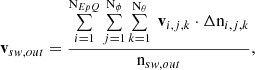
Now, we extend our approach to all three directions and consider the 0th, 1st, and 2nd moments. To quantify the systematic influence of the instrumental response functions on the derived moments we scanned the inner FoV of PAS; that is, −10° < φsw, in < 0° and −5° < ϑsw, in < 5°. This range, indicated with a rectangular shaded black area in Fig. 3, has been chosen to include the most abundant measured flow directions (compare panel c) of Fig. 4 for φsw, in). For all configurations, i.e. combinations of input direction φsw, in, ϑsw, in and angle αin, the results for all parameters are summarised in Fig. 5. In each panel, the range of deviations (ratios in panels a), c), d), e), and differences in panel b)) between input and output parameter depending on αin are shown. In this section, we still assume an instrument with sufficiently good instrumental sensitivity to be able to observe the input VDF over a full 5σ interval. The effects of a limited FoV and limited instrumental sensitivity are discussed in Sect. 5.
 |
Fig. 5. Over- and underestimation of the 0th (Panel a)), 1st (Panels b) and c)), and 2nd moments (Panels d) and e)) over the respective input angles αin as determined by VPAS. In panels a)–e), the shaded areas represent the full range of results for all considered input configurations. Solid lines correspond to the respective minima and maxima and dots mark the tested αin. Panel e) gives a zoom-in of panel d). In panels a)–e), three regimes (i), (ii), (iii) are indicated with (fuzzy) black vertical lines. Vertical dashed coloured lines indicate the respective grid spacing, ΔGSγ, ΔGSϕ, and ΔGSθ. Panel f) shows the cumulative fraction of occurrence of the angles observed by PAS from 7 July 2020 to 30 November 2023 (valid data with a quality factor of 0 only). A total of 15 476 959 observations is included here. The range of temperature ratios at the regime boundaries in panel e) is translated with Eq. (15) into output angles αout. Shaded coloured regions in panel f) mark the resulting ranges of αout. |
The results for the density nsw are shown in panel a). The shaded red area marks the full range of the ratios nsw, out/nsw, in for all tested configurations. The results can be roughly split into three regimes. In the first regime (i), for αin below the instrumental grid spacing (ΔGSϕ ≈ ΔGSθ ≈ 5°, compare Table 1) the ratio shows a variability ±15%. In the second regime (ii), 5° ≲αin ≲ 11.5°, the density is very well resolved. Further, in this regime, the variability of the results over all tested configurations is small, ≈2%; however, the density is also slightly overestimated by ≈2%. In the next regime (iii), for αin ≳ 11.5°, a systematic decrease in the determined density is observed. At these temperatures already parts of the VDF are outside the FoV of the instrument.
In panel b) the differences in the flow directions, φsw, out − φsw, in and ϑsw, out − ϑsw, in, respectively, are shown. The same three regimes can be determined as for the density. Below 5° (regime (i)) the directions are off by up to ≈1°. As discussed before in the context of Fig. 3 the output flow angles are pushed to the centres of the instrumental bins due to the directional responses. In regime (ii), which is up to αin ≈ 11.5°, both angles are well resolved. In the third regime (iii), above αin ≈ 11.5° in ϑ direction, parts of the distribution are cut off by the FoV (compare Table 1), which leads to a systematic shift of the determined flow angles and to the previously discussed decrease in density. In φsw, in direction, this effect starts to become visible at higher values of αin ≈ 15° than for the ϑsw, in direction.
For the bulk velocity shown in panel c) a small systematic overestimation between ≈0.3 − 1% is observed for αin ≲ 11.5° (regimes (i), (ii)). From that point on, a slight systematic increase in the determined bulk velocity can be seen. This effect can easily be understood by imagining the situation sketched in Fig. 1 for a hotter distribution. For such a hot VDF, systematically parts of the VDF at smaller velocities, i.e. slower than the bulk flow, are cut off by the FoV. This results in an overestimation of the bulk velocity.
The results for the three temperatures are shown in panel d). Not surprisingly the three regimes that have been visible in the 0th moment and the flow directions are also clearly visible in the 2nd order moments. Below the instrumental resolution, in regime (i), systematic influences on the temperatures are strong. In the y and z directions, temperatures can be as much as two orders of magnitude over- and for very cool distributions even underestimated. Temperatures in the x direction are up to one order of magnitude overestimated and no underestimation occurs in this regime for this component. As was discussed before, the differences between the x direction on the one hand and the y and z directions on the other hand, can be explained by the different instrumental directional responses (compare panel g) to panels b) and d) in Fig. 3). The effect of the limited instrumental FoV can be seen in the z direction. In regime (iii), above αin ≈ 11.5°, the temperatures start to be systematically underestimated due to the instrumental cut off at the edge of the FoV. However, the most surprising and striking finding is the behaviour of the temperature in the regime (ii) in-between, which can be seen best in panel e) that shows a zoom in of panel d) with a linear axis: all temperatures are systematically overestimated in this regime. Here, we assumed an instrument with a good instrumental sensitivity. As discussed in Sect. 5, a limited instrumental sensitivity introduces an additional source of underestimation for the temperatures.
Further, in these artificial measurements, the input VDF is isotropic. Nevertheless the measured temperatures always indicate strong anisotropies, simply because the instrumental limitations in terms of grid-spacing driven resolution and limited FoV are not the same for the different directions. We emphasise that we find no range where temperatures are determined without systematic errors. This observation has important implications, for example, for all temperature anisotropy studies. If the measurement is rotated into a magnetic field aligned coordinate system, this effect is compounded and for the same isotropic VDF different apparent temperature anisotropies would be measured for different magnetic field directions.
Panel f) puts the results of VPAS in the context of how frequently the different temperature regimes are observed with PAS. To this end, the variability of the temperature ratio at the regime borders is translated into a range of angles for each direction with Eq. (9). The resulting ranges are indicated with shaded green, blue, and orange areas in panel f). In addition, panel f) shows the cumulative sums of PAS observations in all three directions. This shows that for all three directions, regime (i), which exhibits severe overestimation of temperatures, is expected in 15–20% of all PAS observations. About 65 − 70% of all PAS observations fall in regime (ii), for which significant and direction dependent overestimation is expected based on VPAS. Thus, the deliberations of this section are highly relevant for the majority of PAS measurements and the majority of the observed temperatures are systematically overestimated.
5. Theoretical limits of a finite resolution detector
With VPAS, in the previous section an instrument with a well known calibration has been investigated. Now, we further idealise our virtual detector to investigate the influence of a finite resolution, i.e. a finite grid spacing. In detail, the measurement errors of idealised box-shaped response functions on measured temperatures under the assumption of thermal velocity distributions are examined. We refer to this as the Finite Resolution Detector (FRD) in the following. As we show in this section and Appendix E this is equivalent to the question of at how many equidistant points a standard normal distribution has to be sampled to determine the 2nd moment reliably.
The mathematical description and numerical details of this model are outlined in Appendix E. The analysis is based on a 1D model with an infinite number of bins, i.e. the FoV is unlimited and the measured distribution is not cut7. In this section, we express the velocity, v, in units of the thermal velocity, vth, in, as w = (v − vsw, in)/vth, in with vsw, in = 0. The FRD is defined by its bin spacing with respect to the width of the simulated distribution, i.e. the number of bins per sigma NBpS = 1/Δw with Δw as the constant distance between two consecutive bin centres wi and wi + 1. The response,  , of the ith bin wi is set to
 (21)
(21)
i.e. an idealised box-shaped response is given. This model is valid for all thermal distributions without loss of generality (w.l.o.g.) and by definition exactly reproduces the density, i.e. nsw, in = nsw, out. The only degree of freedom of the input VDF is the inflow direction, wmin, with respect to the instrumental bins, which is defined by the position of the closest bin centre to the centre of the VDF. The model can be evaluated for different NBpS and for different inflow directions wmin. I.e. for wmin = 0, the bulk flow exactly matches one of the instrumental bin centres, and for wmin = ±Δw/2 the bulk flow lies exactly between two bins.
Panels a) and b) of Fig. 6 illustrate how an input 1D Maxwell-Boltzmann distribution given by Eq. (E.2) (in red), is scanned by the FRD. In panel a) NBpS = 0.5 and wmin = 0.2Δw, and in panel b) NBpS = 1.0 and wmin = −0.3Δw have been chosen as examples. The horizontal dashed blue lines show the resulting partial densities calculated according to Eq. (E.9). The resulting velocity distribution according to the moments calculation using Eqs. (E.10)–(E.12) are shown with solid blue lines.
According to Eq. (E.2), our input parameters are nsw, in = 1, wsw, in = 0, wth, in = 1. The resulting moments are nsw, out = 1, wsw, out = 0.004, wth, out = 1.150 (Panel a)), and nsw, out = 1, wsw, out = 0.000, wth, out = 1.0418 (Panel b)). As expected from Eq. (E.10), the density is determined exactly in both cases. The error of the bulk velocity measurement is 0.4%, and smaller than 0.05% for the thermal velocity vth for panels a) and b), respectively. However, the corresponding errors in temperatures are given by  , which is 32.5% and 8.3% for panels a) and b), respectively. The error of the bulk velocity basically stems from wmin, i.e. how symmetric the distribution is sampled. Naturally this error propagates into the 2nd moment. However, this is not the main source of error for the 2nd moment. Although the densities Δni are integrated correctly over the bins, the bin centres wi are not the centres of gravity of the VDF in each individual bin. Thus, the assumption that the bin centres, wi, that go into Eq. (E.12) represent the centre of gravity of the measurements in this bin is violated for a Maxwellian distribution. This assumption would only hold for VDFs that are symmetric to the bin centres within each bin. For the case of a thermal distribution, the monotonically decreasing density in the flanks of the distribution naturally leads to an overestimation of the temperature.
As was described above, the FRD is only restricted by its finite bin width, and thus the resulting moments derived from its artificial measurements only depend on NBpS and wmin, i.e. the temperature (vth, in) and the inflow direction (vsw, in). This dependency is discussed in Sect. 5.1. The additional effects of a limited FoV (such as those seen for VPAS and SPAN-I) and of a limited sensitivity are addressed in Sects. 5.2 and 5.3, respectively.
5.1. Influence of finite resolution
To investigate the errors caused by the finite resolution of a detector systematically, the moments were computed for different NBpS. For each NBpS, inflow directions in −Δw/2 ≤ wmin ≤ Δw/2 were evaluated. Since for a detector with unlimited instrumental sensitivity, the errors of the 1st moment are already well below 1% of vth, in, in this section we focus on the errors of the 2nd moment, or more precisely on the ratio  . The ranges of derived temperature ratios are presented in blue in Fig. 6c).
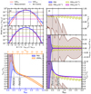 |
Fig. 6. Scaled differential densities in panels a) and b). In red, a standard normal distribution with zero mean and σ = 1 is shown. Dashed black lines mark bin boundaries for two grid spacings: a) NBpS = 0.5, b) NBpS = 1. FRD results are presented in blue. Bin integrated mean values (steps) and the distribution determined from a moment calculation (line) are shown. Blue and red crosses mark the values at the bin centres. In panel c), the ratios Tout/Tin of the respective FRD over NBpS are shown in blue. The results for Ty, out/Ty, in of the VPAS are included in orange. The αin axis on the top of panel c) is scaled to approximately match the scale of NBpS. The dashed lines mark the NBpS values from panels a) and b), respectively. Coloured horizontal lines in panels a) and b) mark three effective thresholds, e.g. FRDLS(10−1) in brown. For these three thresholds and for the FRD panel d) shows the density ratio nsw, out/nsw, in, panel e) gives the velocity difference relative to the thermal speed (vsw, out − vsw, in)/vth, in, and panel e) provides the temperature ratio Tout/Tin in the same scaling as panel c) (but with a lower upper limit). |
Below NBpS ≈ 0.5, even the idealised FRD is not capable of resolving temperatures. For NBpS > 0.5, the unavoidable errors due to finite resolution decrease from ≈33% at NBpS = 0.5 over ≈8% at NBpS = 1.0 to smaller than 1% at NBpS = 2.9. For the design of future instruments, we therefore suggest defining the requirements such that NBpS ≥ 2.9 is ensured for the temperatures of interest.
In addition to the FRD results, the results of Ty, out/Ty, in for VPAS (see Fig. 5) are shown in orange in Fig. 6c). The abscissa is scaled by a factor of 1/(2ΔGSϕ) to approximately match NBpS, under the assumption of the average resolution of PAS from Table 1. Note that compared to Fig. 5, Fig. 6 covers a larger range of αin. The errors of VPAS follow the trend of the FRD results in the range 0.5 ⪅ NBpS ⪅ 1 where VPAS does not suffer from incomplete coverage of the VDFs but at a higher level and with a larger spread. This behaviour can be explained well by the fact that VPAS does not fulfil the FRD assumptions of non-overlapping uniformly spaced bins and constant phase space coverage,  . The overlapping bins of PAS effectively reduce the temperature resolution and increase the measurement error. Thus, the FRD qualitatively reproduces the results of VPAS and thereby verifies that the finite resolution is indeed the source of the temperature overestimation.
5.2. Influence of limited field of view
For NBpS ⪆ 1 the VPAS results differ from the FRD results. This effect can be understood by retracing the effect of a limited FoV based on the examples shown in panels a) and b) of Fig. 6. A limited FoV would cut off the VDFin (red curve) at a fixed value, i.e. w = 3. This leads to fewer bins that contribute to the moment calculation (bins above w = 3 are outside the FoV and have an expectation value of zero). In addition, the expectation value in the bin that contains w = 3 is reduced. The 0th and 2nd moments are therefore underestimated (compare Eq. (3)). Since the effect of the limited FoV is asymmetric (depending on the position of the VDF relative to the FoV), the 1st moment is more strongly affected than by the other effects discussed in this study.
The magnitude of the effect of the limited FoV and the αin at which it is starting to contribute to the overall systematic error is of course driven by the extent of the FoV. This extent typically differs even between the angular directions of a given instrument, as can be observed in Fig. 5. Here, the temperatures in the z direction for VPAS are starting to become underestimated for smaller αin than in the y direction due to the smaller FoV in z direction. This inhibits the comparability of different temperature components measured by the same instrument. A comparison between different instruments each with different FoVs has therefore to be done even more cautiously.
In conclusion we suggest that the design of the requirements of future instruments should acknowledge this effect. Thus, we call for sufficiently large FoVs to prevent these avoidable systematic errors.
5.3. Influence of instrumental sensitivity
The only limitation of the FRD is the finite width of its bins and its results only depend on NBpS and wmin, i.e. the temperature (vth, in) and the inflow direction (vsw, in). To investigate the impact of a limited sensitivity of an instrument, i.e. the capability of resolving small densities in a given grid spacing, the scenario of the FRD is modified in this section. The FRD is based on expectation values and thus does not depend on the density nsw, in, i.e. the sensitivity is unlimited. This means that even the smallest signals are taken into account by the FRD. But every real instrument has a lower and an upper detection limit. For PAS-like instruments, these limits are the lowest and highest number of counts that can be recorded. Therein, the lower limit is well defined by a single count. Other instrument also have a limits. For example, for Faraday cups these are determined by the lowest currents above the noise level and the highest currents that can be measured. In addition, these small signals (i.e. small number of counts or signals close to the noise level) carry systematic uncertainties due to discretisation and large statistical uncertainties. While the latter two effects are not covered in this work (in part since they are largely dependent on the detailed instrument properties), in the following, we investigate the effect of only a lower limit in the measurements on the resulting moments. As an example, we consider a PAS-like instrument that measures single particles, but the result are also valid for other instruments.
An instrument that measures individual particles has an inherent lower limit of a single count. If we take the measurements of the FRD as expectation values for the number of measured particle events, the actual number of expected counts is given by the unscaled density, which is the scaled density shown in Figs. 6a), b) multiplied with nsw, in/vth, in. Thus, for a given vth, in, or NBpS respectively, the total number of expected counts and the expected number of counts in the individual bins scale with nsw, in. The fixed lower limit of a single count can then be realised by setting the expectation values of all bins with an unscaled expectation value smaller than one to zero. We implement this lower limit directly in the scaled density of the FRD, where the lower limit still corresponds to a single count but the effective threshold is given by the scaling factor vth, in/nsw, in. We refer to the resulting model as Finite Resolution Detector with limited sensitivity (FRDLS) with an effective threshold vth, in/nsw, in. We emphasise that different effective thresholds correspond to a single instrumental sensitivity and their spread at a given NBpS reflects the dependence of the expected values on the range of densities that the instrument has to observe.
In Figs. 6a) and b) horizontal solid coloured lines show three effective thresholds of 10−1 (brown), 10−2 (olive), and 10−3 (magenta). The expectation values of each instrumental bin, indicated by blue crosses, below these lines are set to zero. Figs. 6a), b) shows that with increasing effective thresholds, i.e. with an increasing ratio vth, in/nsw, in more bins in the flanks of the distribution are below the effective threshold. As a rough guideline, these effective thresholds illustrate the limitations of a solar wind instrument that observes an input VDF with a total number of ≈10, 100, and 1000 counts respectively. The 0th, 1st, and 2nd moments resulting from the FRDLS for the same three thresholds are shown in panels d), e), and f) of Fig. 6, respectively. These results can be directly compared to the results of the FRD with unlimited sensitivity, which are shown in blue, and the differences show the systematic effects that are introduced by the limited sensitivity.
The sawtooth patterns observed for all three effective thresholds occur if the expectation values in individual bins cross the respective effective threshold. As was expected, for all three moments the deviations from the FRD are stronger with increasing effective thresholds, and thus with worsening sensitivity. While the 0th moment is reproduced by the FRD with unlimited sensitivity perfectly, an increasing effective threshold results for an FRDLS in systematic underestimation of the derived density. For the 1st moment (given in panel e) in units of the thermal speed vth) the effect of an effective threshold is symmetric and is small compared to the thermal speed. Again, the 2nd moment is more strongly affected than the density and velocity. Here, limited instrumental sensitivity leads to a strong underestimation of the temperature. Depending on the effective threshold, the resulting temperature underestimation can even be dominant compared to the overestimation arising from the finite grid spacing. For both the density and temperatures, the results show a trend of increasing underestimation with increasing NBpS. This is also to be expected as the VDF is distributed over an increasing number of bins with increasing NBpS and thus the expectation values of individual bins are more likely to be below the effective threshold. For all three moments an effective threshold of 10−3 already reproduces the properties of the input VDF well.
We focus here on the effect of the lower limit of the instrumental sensitivity. Although not shown here, we expect a qualitatively similar behaviour for the upper limit in the 0th and 1st moments compared to the lower limit. In the 2nd moment, an upper sensitivity limit can also lead to an additional overestimation.
In Sect. 5.1 we suggested an instrument with NBpS ≥ 2.9 to achieve a systematic error of less than 1% for the derived temperatures (based on its finite resolution). For this grid spacing, the effective threshold of 10−3 leads to a systematic error due to the limited sensitivity (see Fig. 6f)) in the same order. However, the dynamic range of the to-be-observed solar wind plasma has to be considered here. If a dynamic range in the temperatures of 100 is to be resolved by an instrument, this translates to a dynamic range of 10 in vth, and thus the NBpS of the above considered instrument increases to NBpS = 29 for a solar wind stream with temperature 100 times higher than before. While this further decreases the systematic error due to the finite resolution, the detrimental effect of the limited sensitivity increases due to the now smaller bin sizes relative to the distribution and the resulting smaller expectation values. In this case, for the effective threshold of 10−3 the systematic error increases to about 15%. Hence, the limited sensitivity of a real instrument affects high temperatures more strongly than lower temperatures under otherwise identical solar wind conditions. The design of future instruments should reflect this finding and the uncertainties should be carefully characterised and quantified based on the detailed design in the early stage of development. Even considering a high dynamic range, the systematic errors from the limited sensitivity should remain in the range of the systematic errors from the finite resolution of the instrument.
For a real instrument, the effective threshold depends on the combination of the solar wind density and temperature. For example, for a fixed temperature, a varying density is reflected by different total numbers of counts that cover a larger or smaller part of the underlying VDF. This effect limits the comparability of temperatures measured by the same instrument for different densities.
5.4. Finite resolution detector summary
With the idealised FRD, we showed that the finite resolution alone is sufficient to introduce an overestimation of the temperature. Only for high resolution (here, NBpS ≥ 2.9) small errors (below 1%) in the temperature measurement can be achieved. However, this also requires a large FoV, as is illustrated for VPAS, which does not reach this regime before the effect of a too small FoV already leads to an underestimation of the temperature. Limited instrumental sensitivity introduces a second source of temperature underestimation that varies with the input density.
In fact, without the limited FoV and limited instrumental sensitivity and the resulting cut-off of the distribution, the overestimation of the temperatures for VPAS would remain above that of the FRD. However, if the resolution of VPAS would have been six times higher with similar shaped response functions and the effective sensitivity threshold is 10−3 or better, the resulting instrument would operate in a regime with an approximately constant but small temperature overestimation. This overestimation would still be position-dependent due to the effects of the non-uniform and overlapping responses. However, for the 15–20% of all PAS observations cases below the instrumental resolution (see regime I Fig. 5f)) we estimate that the resolution would need to have been even > 10 times higher.
The interplay of the three different effects, finite resolution, limited FoV, and limited sensitivity, with their different dependencies and resulting over- and underestimations clearly demands for in-depth analysis of each instrument’s capabilities. All three effects contribute systematic errors that are superposed in the measurements. Although occasionally the overestimation due to the finite resolution and the underestimation due to limited FoV or limited sensitivity can be in the same order, i.e. Tout ≈ Tin, this must not be confused with a mitigation of these systematic effects. The combination of the three systematic errors depends sensitively on the varying solar wind conditions and without full a priori knowledge of the input VDF it is not feasible to identify in a given observation which of these effects contributed exactly to which degree.
A forward-modelling approach, as is suggested in Nicolaou et al. (2025), is useful in this context but requires a model that is flexible enough to describe the measured VDF accurately. For the collisionless solar wind, a simple (bi-)Maxwellian model would be insufficient. We emphasis that these effects can only be mitigated by design and cannot be corrected for afterwards without very strong assumptions about the underlying VDFs.
Our findings hold true for previous missions and their corresponding data analysis as well as for proposed future solar wind instrumentation. In detail, the design of the latter should reflect that the coldest to-be-observed temperatures drive the systematic errors due to the finite resolution while the hottest to-be-observed temperatures (and smallest to-be-observed densities) drive the systematic errors due to the limited sensitivity.
6. PAS versus SPAN-I data
In the previous sections, we have investigated the impact of the instrumental resolution on derived solar wind moments. For the case of PAS we have shown that especially the 2nd moments, i.e. temperatures, are systematically overestimated if the VDFs are inside the FoV. The case of the FRD shows that an overestimation of temperatures is a generally expected feature that arises even under idealised conditions from the finite resolution. The data presented in Fig. 2 shows that SPAN-I temperatures have similar features compared to PAS. However, these data cannot be compared directly, because PAS and SPAN-I measure at different places and times. The radial evolution of the solar wind and the solar activity cycle especially do not allow for a direct comparison of measurements taken at different distances to the Sun or under different solar activity.
6.1. Data selection and influence of frame of reference
To select comparable datasets with respect to solar modulation and radial evolution of the solar wind we applied the following criteria for the comparison in this section. For further details on the data selection see Appendix D. We chose data from both instruments that were taken between 1 January 2022 and 28 July 2023 within 0.3 and 0.5 AU (see Fig. 7a)). These data were further split into vsw intervals of 10 km/s width from 350 km/s to 550 km/s Figs. 7b)–d) shows the distribution of observed solar wind speeds in SRF and RTN and each of these panels highlights one example vsw interval. Similarly to Fig. 5f) the cumulative fractions of observed αx, obs, αy, obs, αz, obs were derived (see Figs. 7f)–k)). Therein, the cumulative fractions for each velocity bin are represented individually, i.e. each line represents a 10 km/s bin. A thicker line marks the velocity bin illustrated in panels b)–e). We refer to the cumulative fractions as distributions in the following.
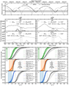 |
Fig. 7. Comparison of PAS and SPAN-I for 1 January 2022 and 28 July 2023. a) Orbits of PAS and SPAN-I. The selection of radial distances (0.3 AU–0.5 AU) that is applied in the panels below is marked with grey shading. Panels b)–e) frequencies of occurences of solar wind velocities in SRF and RTN. An example of a single velocity bin selected based on |


In this section, we specify the frame of reference for the solar wind velocities since here SRF and RTN play a role. As is illustrated in Fig. 1, α depends on  , which is different from the real solar wind speed, v
 . Differences in the data from the two instruments based on a selection for certain
  alone are likely a combination of instrumental effects and physical differences; for example, the effects of mixing different solar wind regimes. However, comparing data for certain
  mixes data observed by instruments on different spacecrafts with variable
  and thus the same temperatures will appear at different values of α in the instrument. Here, we aim to disentangle effects arsing from physical and instrumental differences in the observations of PAS and SPAN-I. Thus, the selection based on vsw has been made twice: On the left side of Fig. 7 in panels b), d), f), h), j) the results for the selection based on
  and on the right side in panels c), e), g), i), k) the results for the selection based on
  are shown. The mixing of the velocities in these two FoRs due to the respective spacecraft eigenvelocities can be seen for one example vsw-bin in panels b)–e). In panels b) and d), the velocity bin in SRF
  (dashed lines) is populated by two distinct populations of solar wind speeds in RTN for both instruments (solid lines). This behaviour is expected due to the spacecrafts’ eigenvelocities. The respective spacecraft eigenvelocities change over the orbit (see panel a)) and are for PAS and SPAN-I at the selected positions larger than the chosen bin width of 10 km/s. Since data from all orbits can be selected, for each selection (based on
  in panels b) and d)), the resulting selection includes data observed under different spacecraft eigenvelocities. In particular, the dataset contains observations that were made while the spacecraft was heading ‘inwards’ or ‘outwards’. Depending on the selection criteria and the spacecraft direction, this reduces or increases the determined velocity in the respective other FoR by ≈25 km/s (for PAS) and ≈40 km/s (for SPAN-I). This leads to the double peak structure in panels b)–e) wherein SPAN-I shows a larger split between the two peaks in each of the panels (solid lines in panels b) and d), dashed lines in panels c) and e)) due to the higher eigenvelocity. The dotted lines in panels b)–e) indicate the respective frequencies of occurrence per velocity bin. These differ between PAS and SPAN-I because of the respectively different time resolutions. In particular, for SPAN-I the time resolution depends on the position in the orbit and therefore, even if the same solar wind stream is observed by PAS and SPAN-I this results in different numbers of individual observations within this solar wind stream.
The comparison of the left and right column in Fig. 7 allows one to assess the influence of the FoR and thereby the influence of physical differences between the observations of PAS and SPAN-I on the following discussion. For both instruments and for all three components, the individual distributions are similar on the left and right side, i.e. for the selection based on  and
and  . Notably, the differences between both sides are smaller than the differences between the two instruments. Also, the spread between distributions of the individual bins on each side are similar. If the comparison was dominated by physical differences in the solar wind plasma observed by PAS and SPAN-I, respectively, we would expect to see differences between the selection based on
  , that mixes different physical conditions, and the selection based on
  , that mixes different instrumental conditions. That the results for both selections are similar indicates that any underlying physical differences are not the main driver for the following discussion. It is highly unlikely that PAS has seen much colder wind than SPAN-I over several orbits and through all solar wind speeds. Therefore, we consider the differences between the instruments and their direction dependent responses as the main drivers for the differences in the observed distributions.
6.2. PAS: Differences between the three components
With the data selection as described above, on average all resulting cumulative fractions of  ,
,  ,
,  and
and  ,
,  ,
,  shown in panels f)–k) are expected to be similar with respect to comparing different components and different instruments. However, panels f)–i) in Fig. 7 exhibit remarkable differences between different components and different instruments. In this section, we discuss the differences between the angles α observed by PAS in all directions.
For PAS the distributions of the angles  ,
,  ,
,  are qualitatively similar for all three Cartesian directions. For each direction, shaded coloured areas show the ranges ΔGSγ < αx < 2ΔGSγ, ΔGSϕ < αy < 2ΔGSϕ, ΔGSθ < αz < 2ΔGSθ. These ranges roughly correspond to regime (ii) in Fig. 5 and to the range bounded by NBpS = 0.5 and NBpS = 1, which correspond to the two examples shown in Fig. 6. However, Fig. 7 shows a different behaviour for the PAS x direction than for the y and z directions relative to the respective resolution. While for the y and z directions the coloured ranges cover a large part of the PAS observations, for the x direction, the green range lies left of the green curves in panels f) and g). Based on the analysis in Fig. 5e), in addition to the effect of the finite resolution, that predicts an overestimation in the shaded green area, the observations of the temperature in the x direction are also overestimated due to the strong overlap of the instrumental responses. Unlike for the y and z directions for which the response functions of two neighbouring bins overlap, for the x direction the response functions of three neighbouring bins overlap (see Fig. 3), which leads to a stronger additional overestimation.
For larger angles α, i.e. to the right of the coloured ranges, temperatures are underestimated due to the instrumental cut-off. As already shown in Sect. 4.2, this underestimation is initially smaller than the overestimation-effect from the finite resolution but eventually becomes the dominant effect. In addition, for such high temperatures it has to be taken into account that – in contrast to SPAN-I – PAS and many similar instruments (e.g. McComas et al. 1998; Schwenn et al. 1975) are not capable of separating solar wind He2+ from solar wind protons without post-processing and additional assumptions. From the principle of operation of PAS the distribution of solar wind He2+ is measured at higher values of (E/q)i than the proton distribution. Further, the He2+ VDF is expected to mix with the proton VDF for high temperatures. If solar wind protons and He2+ were not separated from each other, this would lead to an additional overestimation of the proton temperatures. To derive proton temperatures, frequently a cut in (E/q)i is applied to the data to separate both species. Such a cut effectively reduces the FoV for proton measurements further and can therefore lead to a systematic underestimation of higher proton temperatures similar to the limited FoV in y and z direction as discussed in the previous sections. Therefore, temperatures derived from data of an instrument that is not capable of separating solar wind protons from He2+ are either overestimated or underestimated depending on whether or not and how exactly such a cut in the data is performed.
For the y and z directions, the behaviour in Fig. 7 is well described by the regimes introduced in the previous sections. A small fraction of the observations gives temperatures below the grid spacing, ΔGSϕ and ΔGSθ, respectively; that is, in the regime of the arc-like structures in Figs. 2, 3, and 4. A large fraction of observations falls in the intermediate regime where all temperatures are overestimated as a result of the interaction between finite resolution and overlap of response functions. The third regime, in which underestimation due to the limited FoV plays a role and eventually becomes dominant, is also populated by the PAS observations.
The additional and variable underestimation due to limited instrumental sensitivity likely affects observations in the second and third regime. Since this underestimation depends on the solar wind density (and due to the fixed scan time per (E/q)i and elevation step also on the solar wind velocity), for denser solar wind (i.e. slow solar wind compared to coronal hole wind or observations close to the Sun compared to further away from the Sun) the effective instrumental effect is more likely an overestimation of the temperature than for less dense solar wind (i.e. coronal hole wind or observations further away from the Sun) for which the effective instrumental effect is more likely an underestimation of the temperature.
6.3. SPAN-I: Differences between the three components
In this section, we focus on differences between the SPAN-I distributions in the three directions. For SPAN-I the distributions in  ,
,  ,
,  are distinctly different for all three Cartesian directions. Since we do not have access to the full calibration information for SPAN-I, we here only mark the expected lower limit of regime (ii) with vertical dashed grey lines8. For small angles α in the x and z directions, the SPAN-I distributions are distinctly different from each other. The distribution in the x direction starts to rise at smaller α values than in the z direction. Similarly to the x direction for PAS, the vertical dashed grey line that indicates the grid-spacing ΔGSγSPAN − I in the x direction and correspond to the top of the arc-like structures discussed in the previous sections are located left of all SPAN-I observations. In the z direction the rise matches the expected position above the arc-like structures; that is, the grid spacing ΔGSθSPAN − I in z direction. Further, the rise in the z direction is steeper than in the x direction. This corresponds well to the different resolutions in these two directions. Due to the coarse resolution in z direction very low temperatures (regime (i)) cannot be resolved and the overestimation of low temperatures in regime (ii) is strong. At higher temperatures the distributions in the x and z directions become more similar.
For the y direction Livi et al. (2022) and Kasper et al. (2020) state that temperatures are not reliable and are systematically underestimated due the partial coverage of the VDFs caused by SPAN-I’s position behind PSP’s heat shield. This effect can be seen clearly in the data in panels h) and i). Basically all observations in these panels show temperatures at the edge of the instrumental resolution ΔGSϕSPAN − I. The upper bound for the temperature in the y direction is a direct consequence of the incomplete coverage of the VDF in this direction as discussed in Livi et al. (2022). The main cause for the lower bound on α is most likely a very large overlap of the responses of the higher-resolution anodes for pairs of neighbouring bins in ϕ direction of SPAN-I, as described in Fig. 6 in Livi et al. (2022). Similar to the situation in the x direction for PAS (see Fig. 4), we expect the strong overlapping responses to result in a minimum  close to ΔGSϕSPAN − I.
6.4. Comparison of PAS and SPAN-I
Even under conditions that are as similar as possible, PAS and SPAN-I observe systematically different angles, α. The y direction is not considered in this subsection because of the previously mentioned well-documented partial coverage of SPAN-I in this direction.
In the x and z directions, the respective distributions of SPAN-I are all shifted systematically to higher angles α compared to PAS. In the z direction this shift is most striking: here almost all angles  observed by SPAN-I are larger than 15° whereas almost all angles
  observed by PAS are smaller than 15°. Nevertheless both instruments exhibit a similar behaviour relative to their respective grid spacing and their differences can be explained by the different respective resolutions in terms of grid spacing and overlap of the respective response functions.
On the one hand, for small angles α the coarser grid spacing of SPAN-I probably leads to a stronger overestimation of temperatures in SPAN-I compared to PAS. On the other hand for large angles α, the smaller FoV of PAS leads to a stronger underestimation of temperatures for PAS than for SPAN-I. Thus, neither instrument is perfectly suited to capture the full range of temperatures occurring in the solar wind. For small angles α, PAS provides a more realistic picture while for large angles α SPAN-I is probably closer to the physical temperatures than PAS. However, even in the regimes where each of the instruments provides a more realistic measurement than the other instrument, we still expected respective over- and underestimation of the real solar wind temperatures. The underlying distribution of solar wind temperatures covers likely a broader range than the combined PAS and SPAN-I measurements.
7. Summary and conclusions
We have investigated the influence of the detailed responses of solar wind instruments on derived solar wind parameters nsw, vsw, and T. We distinguish here between different aspects of the instrumental resolution, i.e. the grid spacing, a bin-specific width of the instrumental response function, the overlap between response functions of neighbouring instrumental bins, and the detailed shape of each response function. As test cases for our study, we chose two of the most modern solar wind instruments, PAS and SPAN-I. However, qualitatively our results can be transferred to all similar instruments.
We find clear signatures of instrumental effects in the data of PAS and SPAN-I that can be reproduced for PAS by a virtual detector, VPAS. As input for VPAS, we chose a simple thermalised Maxwellian and characterised how its temperature is seen in the instrumental FoR. To this end, we defined an angle, α, which allows for temperatures to be directly compared to the instrumental resolution.
While the density and bulk velocity of a thermalised Maxwellian VDF can be accurately determined for the majority of measurements, our model shows that temperatures suffer from systematic over- and underestimations that are caused by two competing instrumental effects.
-
Overestimation occurs due to the insufficient resolution of the instrument. The comparison of PAS and VPAS implies that 80–90% of PAS data suffers from this overestimation. The lowest observed temperatures (15–20% of PAS data), in particular, fall into the range where the instrument is not capable to resolve these temperatures at all. Our analysis implies that the temperatures of this particular cold solar wind plasma are even lower than what was reported previously in the literature. The lower bound of resolvable temperatures is determined not only by the grid spacing but also by the detailed shape of the response function, in particular the overlap of neighbouring bins. But even above this lower bound temperatures are systematically overestimated by 10–50%.
-
The main cause of underestimation lies in the limited FoV and limited instrumental sensitivity. If parts of the VDF do not fall into the FoV, this contributes to an underestimation effect for the density and the temperatures. Based on VPAS, we estimate that 10–20% of the PAS data are affected in this way. Limited counting statistics driven by the instrumental sensitivity and the measurement time additionally reduce the effective FoV. Hence, the upper bound of the resolvable temperatures is driven by the combination of instrumental FoV and the sensitivity. The underestimation caused by this additional reduction of the FoV is a systematic error and is not to be confused with the statistic uncertainty.
Based on the comparison of VPAS and PAS, we conclude that all PAS temperatures are affected by one or both of these effects. Both effects also depend on the location of the VDF in velocity space with respect to the instrumental bin centres and the limits of the FoV. Since PAS, similarly to other solar wind instruments, features different instrumental resolutions in different directions, each direction is affected by its own combination of over- and underestimation. For example, while the errors for the temperatures in the y and z directions are dominantly driven by the grid spacing in the respective angles, the errors for the temperature in the x direction are more strongly affected by the overlap of the response functions of neighbouring bins.
We augmented our VPAS approach with a further idealised detector that shows that the above mentioned overestimation effect is a general property of any detector applied to a thermalised Maxwellian VDF. Specifically we show that approximately three samples per thermal speed are needed for a target error of 1% of the temperature. We also illustrated the effect of a limited instrumental sensitivity, which represents an additional source of underestimation that sensitively depends on the solar wind conditions, in particular the density. As a result, solar wind temperatures determined under different density conditions are not directly comparable. Further, the theoretical perspective suggests that a much finer grid spacing (i.e. by a factor > 10 finer), together with a larger FoV and good and constant instrumental sensitivity, would have allowed PAS to resolve not only the density and speed but also the temperature accurately and independently of the solar wind conditions.
In a systematic comparison of PAS and SPAN-I data under similar conditions (i.e. solar activity, distance to the Sun, solar wind speed), we found striking differences. Both PAS and SPAN-I are strongly affected by the instrumental effects arising from the finite resolution (grid spacing) and the overlap of response functions of neighbouring bins. For low temperatures SPAN-I is more strongly limited by its resolution than PAS, whereas for high temperatures PAS is more strongly affected by its smaller FoV than SPAN-I. The effect of the instrumental resolution is so strong that almost all temperatures observed by SPAN-I are above the highest temperatures observed by PAS. The underlying distribution of solar wind temperatures likely covers a broader range than the combined PAS and SPAN-I measurements. Specifically, the comparison between PAS and SPAN-I shows that different solar wind types are affected by a different combination of over- and underestimation, even under the same solar wind conditions. Therefore, a simple instrument-independent guideline to quantify the systematic instrumental errors is not feasible.
Before we discuss the implications of our findings, we first argue that the results of our study can be generalised from our assumptions (e.g. thermalised Maxwellian VDF and moment calculations). For our virtual detector approach, we used a simple single thermalised Maxwellian VDF. This represents a minimum requirement that is – as we have illustrated in this study – already challenging and requires for temperatures a high resolution that has not been realised in any solar wind instrument. However, the solar wind is frequently not in thermal equilibrium, consists of multiple particle populations, and exhibits several other non-thermal features (Marsch 2006). Capturing these features in solar wind measurements necessitates an even higher resolution than for the simple thermalised Maxwellian case discussed here.
In addition, the observed VDF is often rotated into a magnetic field-aligned coordinate system. If the resolution of the measured VDF is different for different directions in the instrumental frame, such a rotation then mixes the different resulting errors and thereby further distorts the VDF.
In this study, we have considered only the approach to extract solar wind properties from the measured VDF with the help of moments. However, our conclusions also qualitatively transfer to alternative approaches.
All of the observed solar wind temperatures investigated in this study are in one way or the other affected by the instrumental resolution. Thus, our results have far-reaching consequences for the design of future solar wind instruments and past and future studies in heliophysics.
7.1. Implications for the design and data processing of solar wind instruments
We have shown that even the state-of-the-art solar wind instruments PAS and SPAN-I are not capable of resolving the temperature of typical solar wind distributions without introducing significant systematic errors and measurement artifacts. Since these issues are dependent on the actual inflow directions in the SRF, observational biases are introduced that can lead to misconceptions in the interpretation of the data. The differences that arise from the respective different instrumental response functions can under no circumstances be resolved by cross-calibration between different instruments. Further, since the detailed over- and underestimation effects discussed in this study depend on the unknown observed VDF, these instrumental effects cannot be corrected for by post-processing.
We emphasise that PAS and SPAN-I both fulfil their respective design requirements remarkably well. However, given the importance of reliable solar wind temperature measurements (see Section 7.2 for implications on different research topics), we think it is vital to refine requirements for future solar wind instruments and to underline the importance of transparent data processing.
-
A good instrumental resolution for low temperatures implies the following requirements: solar wind instruments must be designed such that their resolution in terms of the finite grid spacing and the overlap of the response functions allows one to determine temperatures of thermalised and non-thermalised distributions in the expected temperature regime. Hereby, the lowest temperature to resolve must not be fully determined by previous measurements that are affected by the limitations discussed in this study. Ideally, this lower limit would be well below photospheric temperatures. As is discussed in Podesta (2015) for small-scale structures in the VDF and in this study for thermal velocities, this would translate to an increase in the resolution by a factor of 10 compared to current solar wind instruments. The desired resolution must be achieved for all considered solar wind speeds and it should be similar for all directions (in order to prevent instrumental bias). An uniform velocity space coverage without gaps and/or overlaps would help to achieve such a resolution.
-
A good instrumental resolution for high temperatures implies the following requirements: solar wind instruments must be designed such that the VDF is sampled at least up to ≈4 − 5σ. To this end, the instrumental sensitivity must be good enough and the FoV must be large enough to avoid density and temperature underestimation. For example, for a PAS-like instrument the sensitivity requirement implies that at least a total number of 1000 counts is required for the lowest to-be-observed densities at the highest to-be-observed temperatures. The upper limit of the temperature requirements is driven by coronal temperatures, and thus should be well above 1 MK.
-
Explicit species separation by measurement design rather than by post-processing is highly preferred to prevent the introduction of additional uncertainties.
-
We strongly support open data policies. Any data reduction and refinement should be made public with all necessary instrumental details being provided to the scientific community. This includes the full data processing chain as well as introduced cuts, correction terms, and of course response functions (such as those of PAS shown in Figure 3). This also holds true for previous solar wind instruments. The response functions should be determined under as flight-like conditions as possible, i.e. stepping through different deflection and EpQ steps should be made in exactly the same mode as in flight. Furthermore, on-board reduction of data should be avoided if possible to prevent any ambiguities that cannot be recovered by on-ground analysis.
These requirements are naturally difficult to implement in a single instrument. Higher resolution will result in increased resource budgets, for example for mass, volume, power, on-board data storage, and data telemetry, and thus increased overall costs. We acknowledge that mission budgets force instrument teams to make design compromises that make each proposed instrument better or worse with respect to different aspects. As a consequence the resulting instrument is better or worse suited for different scientific research questions (see Sect. 7.2 for examples). These challenges could be mitigated; for example, by combining several solar wind instruments that are designed for complementary science goals. Frequently, different instruments are designed to measure different properties of the solar wind; for example, different instruments in the payload are responsible for protons and ions heavier than protons (as for Wind, SOHO, ACE, and Solar Orbiter) and sometimes also several proton plasma instruments that specialise in a high time resolution or better species separation (as for Wind and PSP). We suggest taking this concept further and considering, for example, instruments specialising in different solar wind regimes.
All instrumental limitations must be carefully assessed, clearly communicated, and taken into account in the data analysis. Just as our findings underline the scientific need for higher instrumental resolution, they can also serve as an argument for increased instrumental budgets for future missions.
7.2. Implications for past and future scientific studies and affected topics in heliophysics
The instrumental limitations discussed in this paper are relevant for all studies in heliophysics that directly or indirectly rely on temperature. Thus, past studies (see a list of examples of research topics below) should be revisited and carefully reassessed. As was detailed above, the implications of the instrumental limitations shown here cannot be generalised and are subject to the individual details of a given solar wind instrument and the studied solar wind regimes. Thus, referring to the open data policy requirement in Sect. 7.1, it is in the responsibility of the instrument teams to provide the detailed response and calibration of previous solar wind instruments to the scientific community. Based on that the responsibility to assess the impact of these instrumental details on each individual study lies with the scientific community, i.e. systematic errors and instrumental limitations must be taken into account and must not be overlooked or ignored.
In the following, we provide a list of research topics that we expect to be affected. This cannot comprise a comprehensive list and all topics and references in the following are intended as examples only. From our point of view, most if not all solar wind studies should be revisited in light of the results presented in this paper.
-
Here, we have only considered the 0th, 1st, and 2nd moments of the proton VDF and we have shown that the highest considered moment, i.e. the temperature, is most sensitively affected by the instrumental resolution. Other derived quantities, such as the plasma beta, the collisional age, or the pressure, inherit the errors inherent in the temperature determination. In addition, higher moments, such as the energy flux density, are very likely also affected and even to a stronger degree. Thus, studies investigating other derived quantities and higher moments of the solar wind VDF should also be revisited.
-
The different resolutions in different directions can affect the 1st moment of the VDF, which could be misleadingly interpreted as deviations from a thermalised Maxwellian VDF. As Podesta (2015) argues, small deviations from the thermal equilibrium case contain valuable hints about the dissipation of Magnetohydrodynamics (MHD) turbulence (e.g. Vasquez et al. 2007), the identification of waves and turbulence on MHD and kinetic scales (e.g. Marsch 2006), or the angular of momentum loss of the Sun due to the solar wind (e.g. Pizzo et al. 1983). Consequently, our findings are also relevant for these research areas.
-
We find that even for a thermalised Maxwellian VDF, unequal instrumental resolutions in different directions appear as a temperature anisotropy. However, the frequently observed temperature anisotropies in the solar wind have been subject to many studies and are therein for example related to kinetic instabilities (e.g. Marsch 2006; Yoon 2017). In this context, temperature components parallel and perpendicular to the magnetic field direction are of interest and the measured VDF need to be transformed in a respective coordinate system. This transformation introduces non-linear mixtures of the different resolutions and FoV limitations. These effects need to be carefully disentangled to study physical temperature anisotropies.
-
The effects described in the previous point are further amplified if one considers multiple VDFs. Frequently, proton distributions composed of a core and a magnetic field aligned beam are observed (e.g. Marsch 2006). The beam formation is related to wave-particle interactions which are still not well understood. Since details of the distribution matter for wave-particle interaction, the systematic instrumental effects discussed in our study can lead to misleading interpretations. Furthermore, often differential streaming between protons and heavier ions is observed in the solar wind (e.g. Kasper et al. 2008; Berger et al. 2011). In addition to the aspects discussed above, some related studies have utilised solar wind properties from different instruments (e.g. Hefti et al. 1998), which introduces an additional uncertainty due to the individual systematic errors inherent in these instruments.
-
While coronal hole wind is generally considered to be a collisionless plasma, for slow solar wind fewer non-thermal features are observed. This is often interpreted such that in cold, slow solar wind collisions are relevant for the plasma behaviour and the collisional age or Coulomb number is employed as an ordering parameter in the solar wind (e.g. Kasper et al. 2012; Heidrich-Meisner et al. 2020). The collisional age depends on the solar wind density, velocity, and temperature. Thus, it is also affected by the respective instrumental effects and it is questionable whether subtle non-thermal features can be resolved.
-
A long-standing, well-known result in solar wind science is the correlation between the observed solar wind temperature and the solar wind speed. Since the lowest temperature that can be resolved by an instrument scales with the bulk velocity, a similar dependence is expected to result from instrumental characteristics alone. The extent to which such an instrumental contribution accounts for the observed correlation might be worth reassessing, even for this well-known result.
-
Another well-studied property of the solar wind is mass-proportional heating (e.g. Isenberg & Hollweg 1983, and references therein). At the same temperature, vth scales with
 (see Eq. (5)); for example, for helium vth is a factor of two smaller than for protons. Thus, the temperature of heavier ions is even more difficult to resolve than proton temperatures, i.e. we expect that their temperature will be subject to stronger overestimation. Since the systematic temperature overestimation can sensitively depend on the inflow direction, this effect is reinforced if the inflow direction of heavy ions and protons differ from each other. These effects mimic mass-proportional heating and necessitate the re-evaluation of observations and theoretical models of mass-proportional heating.
 -
We have shown that no existing solar wind instrument is capable of resolving very low temperatures. In particular, we have found that for these cold plasma the observed temperatures depend sensitively on the inflow direction. Even small changes in the inflow direction can cause large variations in the observed temperatures without any physical changes. Nevertheless, temperatures below the actual resolution of the instrument are often provided within the datasets. Thus, very low temperatures that are typically associated with very cold, slow solar wind (e.g. Sanchez-Diaz et al. 2016) and interplanetary coronal mass ejection (ICME)s and that are often among the criteria to identify ICME plasma (e.g. Cane & Richardson 2003; Jian et al. 2006; Xu & Borovsky 2015) can easily be misinterpreted.
-
The properties of the solar wind depend on the solar source region and transport effects. Therefore, the proton plasma properties are (together with or instead of charge state compositions) often used to characterise the solar wind and the conditions in its respective solar source region. If the temperatures in the solar wind are frequently overestimated and sometimes underestimated, this affects many of the available solar wind classifications (e.g. Xu & Borovsky 2015; Heidrich-Meisner & Wimmer-Schweingruber 2018) and implies potentially misleading conclusions about the properties of the solar source region. As we have shown, the solar wind temperatures determined by different instruments can be strikingly different. Thus, each solar wind classification including solar wind temperatures is only directly applicable to the instrument it was defined on.
-
The radial profile of the proton temperature for coronal hole wind in the inner heliosphere differs from a naive adiabatic expectation (e.g. Hellinger et al. 2011; Dakeyo et al. 2022). The density-dependent influence of a limited instrumental sensitivity introduces a systematic radial bias for the temperature. Thus, the detailed effect of over- and underestimations of temperatures on radial profiles need to be assessed.
-
In the outer heliosphere, Voyager 2 observed temperatures comparable to the photospheric temperatures (Richardson & Smith 2003) over a large range of radial distances. This unexpected result is explained with additional heating due to pick-up ions (e.g. Chalov et al. 2006). As we show here, the instrumental resolution can lead to a minimum determinable temperature. In this context, the apparent heating could at least in part also be explained by the resolution of the respective plasma instrument and additional pick-up ion heating might not be required or might at least be less important than it is currently believed to be.
-
Shocks occur in the heliosphere in different locations and on different scales (e.g. Lee et al. 2012; Jokipii 2013; Parks et al. 2017), including interplanetary shocks, planetary bow shocks, and the termination shock. They are of particular interest as particle acceleration sites. Shock parameters depend on all components of the velocity vector and the pressure tensor. Since the different velocity and pressure components are affected by their respective different instrumental resolutions, the description of shocks is also affected by the considerations in our study.
-
Although the fleet of active spacecraft in the heliosphere has grown over the last decades, for a global picture large-scale MHD models are currently the only available tool. Such models (e.g. Odstrcil 2003; Pomoell & Poedts 2018) rely on solar wind data in mainly two aspects: as input variables and for their verification. For both aspects, the systematic over- and underestimation of solar wind temperatures are problematic and introduce or reinforce a similar bias in the MHD models. This showcases the importance of incorporating instrumental limitations into models.
Solar wind measurements have driven a rich wealth of studies and research fields from small kinetic scales to the scale of our entire heliosphere. As the examples above illustrate, understanding the systematic limitations and biases that are imposed on solar wind data by the instrumental design and their consequences is crucial for the scientific progress in heliophysics.
Note that we explicitly differentiate between the instrumental properties (ϕ, θ), and the measured angles (φsw and ϑsw).
For PAS metainformation is taken from L1 3D data.
Moment data for a second, finer SPAN-I scan is not available at Kasper et al. (2020). Therefore, we refer here only to the larger but coarser scan.
In practice, the available calibration is an approximation of the instrumental characteristics. We emphasise that the pre-launch calibration should be based on measurements under as realistic conditions as possible, i.e. obtained under the nominal in-flight mode of the respective instrument.
Note that in this section (and this section only), the first arguments of δℛi, j, k and ℰj, k are given as E/q instead of v and the definitions of both quantities are modified to include this substitution.
The reference velocity for γ can be chosen arbitrarily, here we used the velocity of EpQ step, 60 vEpQ, 60.
For numerical reasons we cut at ten sigma.
The responses also depend on the particles mass and charge. For sake of readability we omit additional indices and note that δℛb(v) has to be calculated separately for different ion species.
Note that we use velocity and not momentum space and the limits ±∞ refer to all (non-relativistic) velocities.
Here ΔRW is simply the full velocity bin width where  .
.
Acknowledgments
We thank the German Federal Ministry for Economic Affairs and Energy and the German Space Agency (Deutsches Zentrum für Luft- und Raumfahrt, e.V., (DLR)) for their support through contracts # 50OT2002, 50OO2408, and 50OC2104, as well as Kiel University. We acknowledge the NASA Parker Solar Probe Mission and the SWEAP team led by J. Kasper for use of data.
References
- Bame, S. J., McComas, D. J., Barraclough, B. L., et al. 1992, A&AS, 92, 237 [NASA ADS] [Google Scholar]
- Berger, L., Wimmer-Schweingruber, R. F., & Gloeckler, G. 2011, Phys. Rev. Lett., 106, 151103 [NASA ADS] [CrossRef] [Google Scholar]
- Bosqued, J. M., Lormant, N., Rème, H., et al. 1996, Geophys. Res. Lett., 23, 1259 [Google Scholar]
- Bridge, H. S., Belcher, J. W., Butler, R. J., et al. 1977, Space Sci. Rev., 21, 259 [Google Scholar]
- Cane, H. V., & Richardson, I. G. 2003, J. Geophys. Res., 108, 1156 [Google Scholar]
- Case, A. W., Kasper, J. C., Stevens, M. L., et al. 2020, ApJS, 246, 43 [Google Scholar]
- Chalov, S. V., Alexashov, D. B., & Fahr, H. J. 2006, Astron. Lett., 32, 206 [Google Scholar]
- Dakeyo, J.-B., Maksimovic, M., Démoulin, P., Halekas, J., & Stevens, M. L. 2022, ApJ, 940, 130 [NASA ADS] [CrossRef] [Google Scholar]
- De Marco, R., Bruno, R., Jagarlamudi, V. K., et al. 2023, A&A, 669, A108 [NASA ADS] [CrossRef] [EDP Sciences] [Google Scholar]
- ESAC. 2020, Solar Orbiter Archive SOAR, https://soar.esac.esa.int/soar/, accessed: 2025-03-01 [Google Scholar]
- Galvin, A. B., Kistler, L. M., Popecki, M. A., et al. 2008, Space Sci. Rev., 136, 437 [Google Scholar]
- Hefti, S., Grünwaldt, H., Ipavich, F. M., et al. 1998, J. Geophys. Res., 103, 29697 [NASA ADS] [CrossRef] [Google Scholar]
- Heidrich-Meisner, V., & Wimmer-Schweingruber, R. F. 2018, in Machine Learning Techniques for Space Weather (Elsevier), 397 [Google Scholar]
- Heidrich-Meisner, V., Berger, L., & Wimmer-Schweingruber, R. F. 2020, A&A, 636, A103 [NASA ADS] [CrossRef] [EDP Sciences] [Google Scholar]
- Hellinger, P., Matteini, L., Štverák, Š., Trávníček, P. M., & Marsch, E. 2011, J. Geophys. Res. Space Phys., 116, A09105 [Google Scholar]
- Ipavich, F. M., Galvin, A. B., Lasley, S. E., et al. 1998, J. Geophys. Res., 103, 17205 [Google Scholar]
- Isenberg, P. A., & Hollweg, J. V. 1983, J. Geophys. Res., 88, 3923 [Google Scholar]
- Jian, L., Russell, C. T., Luhmann, J. G., & Skoug, R. M. 2006, Sol. Phys., 239, 393 [NASA ADS] [CrossRef] [Google Scholar]
- Jokipii, J. R. 2013, Space Sci. Rev., 176, 115 [Google Scholar]
- Kasper, J. C., Lazarus, A. J., & Gary, S. P. 2008, Phys. Rev. Lett., 101, 261103 [Google Scholar]
- Kasper, J. C., Stevens, M. L., Korreck, K. E., et al. 2012, ApJ, 745, 162 [Google Scholar]
- Kasper, J. C., Stevens, M. L., Case, A. W., & Korreck, K. E. 2020, PSP Solar Wind Electrons Alphas and Protons (SWEAP) SPC Ion Number Density, Velocity, and Thermal Speed Moments and Fits, Level 3, accessed: 2025-03-01 [Google Scholar]
- King, J. H., & Papitashvili, N. E. 2005, J. Geophys. Res. Space Phys., 110, A02104 [Google Scholar]
- Lazar, M., López, R. A., Shaaban, S. M., et al. 2022, Front. Astron. Space Sci., 8, 249 [CrossRef] [Google Scholar]
- Lee, M. A., Mewaldt, R. A., & Giacalone, J. 2012, Space Sci. Rev., 173, 247 [CrossRef] [Google Scholar]
- Livi, R., Larson, D. E., Kasper, J. C., et al. 2022, ApJ, 938, 138 [NASA ADS] [CrossRef] [Google Scholar]
- Marsch, E. 2006, Liv. Rev. Sol. Phys., 3, 1 [Google Scholar]
- Marsch, E., Schwenn, R., Rosenbauer, H., et al. 1982, J. Geophys. Res., 87, 52 [Google Scholar]
- McComas, D. J., Bame, S. J., Barker, P., et al. 1998, Space Sci. Rev., 86, 563 [CrossRef] [Google Scholar]
- McFadden, J. P., Carlson, C. W., Larson, D., et al. 2008, Space Sci. Rev., 141, 277 [Google Scholar]
- Nicolaou, G., Ioannou, C., Owen, C., et al. 2025, arXiv e-prints [arXiv:2505.09869] [Google Scholar]
- Odstrcil, D. 2003, Adv. Space Res., 32, 497 [CrossRef] [Google Scholar]
- Owen, C., Bruno, R., Livi, S., et al. 2020, A&A, 642, A16 [NASA ADS] [CrossRef] [EDP Sciences] [Google Scholar]
- Parks, G. K., Lee, E., Fu, S. Y., et al. 2017, Rev. Mod. Plasma Phys., 1, 1 [NASA ADS] [CrossRef] [Google Scholar]
- Pizzo, V., Schwenn, R., Marsch, E., et al. 1983, ApJ, 271, 335 [Google Scholar]
- Podesta, J. J. 2015, J. Geophys. Res. Space Phys., 120, 3350 [Google Scholar]
- Pomoell, J., & Poedts, S. 2018, J. Space Weather Space Clim., 8, A35 [NASA ADS] [CrossRef] [EDP Sciences] [Google Scholar]
- Reme, H., Bosqued, J. M., Sauvaud, J. A., et al. 1997, Space Sci. Rev., 79, 303 [Google Scholar]
- Richardson, J. D., & Smith, C. W. 2003, Geophys. Res. Lett., 30, 1206 [NASA ADS] [Google Scholar]
- Sanchez-Diaz, E., Rouillard, A. P., Lavraud, B., et al. 2016, J. Geophys. Res. Space Phys., 121, 2830 [NASA ADS] [CrossRef] [Google Scholar]
- Schwenn, R., Rosenbauer, H., & Miggenrieder, H. 1975, Raumfahrtforschung, 19, 226 [NASA ADS] [Google Scholar]
- Vasquez, B. J., Smith, C. W., Hamilton, K., MacBride, B. T., & Leamon, R. J. 2007, J. Geophys. Res. Space Phys., 112, A07101 [Google Scholar]
- Xu, F., & Borovsky, J. E. 2015, J. Geophys. Res., 120, 70 [NASA ADS] [CrossRef] [Google Scholar]
- Yoon, P. H. 2017, Rev. Mod. Plasma Phys., 1, 4 [NASA ADS] [CrossRef] [Google Scholar]
Appendix A: Remarks on nomenclature
Table A.1 explains the meaning of sub- and superindices in this manuscript. To simplify the notation, indices are omitted wherever that is possible without loss of information. The respective conditions are also specified in Table A.1. For example, thermal properties are always properties of the solar wind bulk and are therefore not indexed with sw.
Further, in Sects. 3-5, all properties are given in SRF and the respective FoV index is omitted. The angle α as defined in Eq. 15 here always refers to SRF (or the instrumental frame) and therefore the respective superindex is always omitted.
Overview on sub- and superindices. The index position defines its respective category.
Appendix B: Relation of temperature T, solar wind speed vsw and angle α
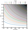 |
Fig. B.1. The solar wind speed dependent conversion from kinetic temperatures T to α is shown. Lines for temperatures in 1 eV steps are shown (black). Some temperatures are highlighted by bold coloured lines. |
Fig. B.1 illustrates the relation (Eq. 9) between the angle α and temperature T for different solar wind speeds vsw. Note that in this study α is calculated in SRF solely, i.e. components of the thermal velocity,  , and the solar wind speed,
  , are used. Only in SRF α can be directly compared to the instrumental resolution.
Appendix C: Instrumental measurement, response, and resolution
The term instrumental response in general is not well defined and different definitions are used in the literature. For the purpose of this study, we define the response, ℛ, as described in the following. We use Cartesian coordinates, but all equations can easily be written in spherical coordinates too. A measurement, μ, of any instrument can be described by
 (C.1)
(C.1)
The density, n, can be obtained from the measurement with
 (C.2)
(C.2)
with a conversion factor of C = 1/ℛ. Here, we denote an instrumental bin with a single subindex, b, as a generalisation from the three indices i, j, k introduced in Sect. 3 for electrostatic analysers. The response of an instrumental bin δℛb(v) for particles9 with velocity v is given by,
 (C.3)
(C.3)
with an effective area, Ab(v), a measurement time, tb(v), and a measurement efficiency, ηb(v). For VPAS and PAS as typical for measured calibrations, η, Ab, and tb are not always determined individually. In Eq. 16, ηb(v)Ab(v)tb(v) = 𝒜b(v)ℰb(v). δℛb(v) is an effective spatial volume from which particles with velocity v are measured. The total response, ℛb, of an instrumental bin is given by integrating Eq. C.3 over the whole velocity space,10
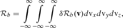 (C.4)
(C.4)
i.e. ℛb is the 0th moment of the response δℛb(v). The measurement within one bin μb is given by,
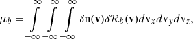 (C.5)
(C.5)
but the inversion of this expression to obtain the density from the measurement requires assumptions about δn(v), i.e. any information about δn(v) except for the weighted integral is lost. Typically the assumption that δn(v) is constant over the range where δℛb(v) > 0 is made, and the inversion according to Eq. C.2
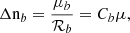 (C.6)
(C.6)
is used to derive partial densities Δnb. In this context ℛb is often referred to as sensitivity of the instrument, as it scales the strength of the measured signal μb for a given density nb. In detail the product t(v)v in Eq. C.3 basically can be regarded as a measure for the combined temporal and the spatial resolution. It determines the length of the spatial volume, which is large compared to the lengths defining the effective area A(v). Thus, the measurement time t(v) is driving both the spatial and temporal resolution of an instrument. The product η(v)A(v) is driving the sensitivity for a fixed spatial and temporal resolution.
For further properties of an instrumental bin typically the responses δℛb(v) are used to describe the centre velocity vb. Often the 1st moment of δℛb(v) is calculated,
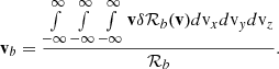 (C.7)
(C.7)
The resolution ΔGS can then be described by the distance between two adjacent bins (in any direction); for example, in the x direction,
 (C.8)
(C.8)
The resolution ΔRW can then be described by the width of the responses δℛb(v). Often ΔRW is characterised proportional to the 2nd moment of δℛb(v) (in any direction); for example, in the x direction,
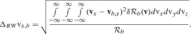 (C.9)
(C.9)
In summary, the attempt to reduce the detailed instrumental responses δℛb(v) to the three quantities sensitivity, central bin velocity and velocity space resolution, is similar to the reduction of the detailed solar wind VDFs δn(v) to the solar wind properties density, bulk velocity and temperature. Consequently, the reduction of measured solar wind VDFs to moments, inherently is based on a second reduction of the instrumental responses to its moments.
Appendix D: Data notes
Selected quality flags for PAS and SPAN-I. If no value is given, no restriction for the respective quality flag is applied in our selection.
As described in Sect. 3, we have taken publicly available PAS and SPAN-I datasets. Table D.1 provides an overview on the chosen quality flags. In addition, in Fig. 7, data with  are omitted to allow for an unbiased comparison of PAS and SPAN-I. These small observed angles
 ![Mathematical equation: $ \alpha_{obs}^{SPAN\mathrm{-]}} $](/articles/aa/full_html/2025/10/aa55609-25/aa55609-25-eq93.gif) correspond to the bases of the arcs in Fig. 2 and comprise 1.3% of the considered SPAN-I data. For PAS most of these very small determined temperatures are assigned non-zero quality flags or they occur for very low solar wind velocities, which are not included in Fig. 7. Such small angles αobs are expected to occur more frequently for SPAN-I than for PAS because of the coarser grid-spacing of SPAN-I compared to PAS.
correspond to the bases of the arcs in Fig. 2 and comprise 1.3% of the considered SPAN-I data. For PAS most of these very small determined temperatures are assigned non-zero quality flags or they occur for very low solar wind velocities, which are not included in Fig. 7. Such small angles αobs are expected to occur more frequently for SPAN-I than for PAS because of the coarser grid-spacing of SPAN-I compared to PAS.
Appendix E: Mathematical background of the finite resolution detector
In this section, we derive the FRD that is used in Sec. 5. We still focus on thermal distributions and, w.l.o.g. we consider 1D VDFs in this section with differential densities δn(v)
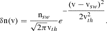 (E.1)
(E.1)
With the scaled velocity, w with  , this can be simplified to a scaled density,
  ,
,
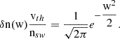 (E.2)
(E.2)
As a standard normal distribution Eq. E.2 has the cumulative distribution function Φ(w)
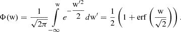 (E.3)
(E.3)
With Eq. E.3 the integral of the scaled density between any lower (w−) and upper (w+) limits can be calculated with
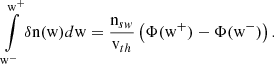 (E.4)
(E.4)
In general any detector measures parts of velocity phase space in a finite number of bins. Following Eq.C.5 the measurement μi of the ith bin is here given by
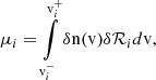 (E.5)
(E.5)
with the limits  and
and  are defined such that
  in v ∈ [vi−, vi+], and
  outside this interval. Now, we assume a detector that covers the whole 1D velocity space with equidistant bins. The distance between ith and (i + 1)th bin is Δv and the lower and upper bin edges are symmetric
  and
and  . Note that this grid spacing differs from the logarithmically spaced bins usually employed in solar wind instruments. This means that the upper bin edge of the ith bin
  is the lower bin edge of (i + 1)th bin
  , i.e. the bins are non-overlapping. For our idealised FRD, we further require
  to be a constant ci within
  and
and  for each bin. The measurement μi in the ith bin is then expressed as
 (E.6)
(E.6)
We choose w.l.o.g. ci = 1 which directly gives us partial densities, Δni,
 (E.7)
(E.7)
Scaling to  and with dv = vthdw we obtain
 (E.8)
(E.8)
And with Eq. E.4, we get
 (E.9)
(E.9)
It holds that the 0th moment nsw can easily be calculated with
 (E.10)
i.e. the density is exactly determined. Now we choose w.l.o.g. nsw = 1, and the 1st moment, wsw, can be calculated with
 (E.11)
and the 2nd moment, wth, with
 (E.12)
The resulting FRD covers the whole velocity space with equal sensitivity and without any overlap. Since for the FRD all velocity bins have the same size, it is fully defined by the constant bin width, i.e. the distance of the bin centres Δw = wi + 1 − wi. In addition, the accuracy of the FRD depends on the inflow direction relative to the bin centres. Because the velocities are scaled to the thermal velocity vth that is the standard deviation, σ, of a thermal distribution we define the number of bins per sigma, NBpS, which is given by
 (E.13)
in units of the standard deviation σ as a measure of the resolution, ΔGS, of our FRD. Thus, by design for the FRD ΔGS = ΔRW11 and the response functions for different bins do not overlap. With the difference that the bins are not equidistant, this is the situation that is illustrated in Fig. 1 in 2D. For a given resolution NBpS, the only uncertainty that is left is how symmetric the velocity distribution is sampled. We define wmin as the position of the bin closest to the global maximum wVDF = 0 of the input VDF as
 (E.14)
The offset of the centres, wmin, can then be chosen such that
 (E.15)
In other words, wmin expresses how close the bulk flow direction is to the nearest instrumental bin. For wmin = 0, the bulk flow exactly matches one of the instrumental bin centres, and for  the bulk flow lies exactly between two bins. These two situations correspond to the bases and the tops of the arcs that have been described in the previous sections (see Fig. 2, 3, and 4).
To investigate the error inherent in the FRD systematically, we computed the 0th, 1st, and 2nd moments for 0.1 ≤ NBpS ≤ 3.0 in 0.1 steps, and vary wmin in −0.5 ≤ wmin ≤ 0.5 in 100 linear steps for each NBpS. The results are shown and discussed in Sect. 4.2.
Appendix F: List of acronyms
ESA European Space Agency
NASA National Aeronautics and Space Administration
SolO Solar Orbiter
PSP Parker Solar Probe
VDF Velocity Distribution Function
PAS Proton Alpha Sensor
SPAN-I Solar Probe ANalyzer for Ions
SWEAP Solar Wind Electrons Alphas and Protons
SWA Solar Wind Analyser
EpQ energy-per-charge
FoV Field of View
FoR Frame of Reference (Not to be confused with field-of-regard) VPASVirtual Detector based on PAS FRDFinite Resolution Detector
FRDLS Finite Resolution Detector with limited sensitivity SRFSpacecraft Reference Frame RTNRadial-Tangential-Normal Frame
MHD Magnetohydrodynamics
ICME interplanetary coronal mass ejection FWHMFull Width Half Maximum
w.l.o.g. without loss of generality
All Tables
Overview on sub- and superindices. The index position defines its respective category.
Selected quality flags for PAS and SPAN-I. If no value is given, no restriction for the respective quality flag is applied in our selection.
All Figures
|
Fig. 1. Example of a 2D cut of a velocity phase-space scan is shown. The black dots mark the central position of instrumental bins (vx, i, j, k, vy, i, j, k) that are scanned, with i ∈ [1, …, NEpQ], j ∈ [1, …, Nϕ], NEQP as the number of energy-per-charge (EpQ) steps and Nϕ as the number of azimuthal bins, the angle of inflow bin ϕj of the jth azimuthal bin, and its corresponding bin width ΔGSϕj. As an example for a solar wind instrument the calibration values of the central elevation bin k = 5 of PAS for protons are used here and in Fig. 3. Note that we explicitly differentiate between the instrumental properties (ϕ, θ), and the measured angles (φsw, obs and ϑsw, obs). All instrumental characteristics are shown in black including the utilised Frame of Reference (FoR). Dots illustrate the shells centred at the origin, i.e. in the Spacecraft Reference Frame (SRF), which are scanned by the electrostatic analyser. Each 5th electrostatic analyser step is enlarged for clarity. The shape of each instrumental bin is illustrated with a concentric grid. The instrumental resolution in velocity space becomes coarser with increasing shell radius. In red, an example of a thermalised Maxwell-Boltzmann VDF (see Eq. (6)) is depicted. Shown are the bulk-flow vector relative to the instrument vsw, its components, vsw, x, vsw, y, and the thermal velocity vth. The corresponding 1σ, 2σ, and 3σ environments of the distribution are indicated in light red. In blue, measurement quantities are shown: the absolute value of the solar wind bulk velocity |vsw|, the y component of the thermal speed vth, y, and the corresponding thermal angle αy. The two relevant FoRs are depicted in the left part of the figure: the SRF in black and the Radial-Tangential-Normal Frame (RTN) frame in green. Therein, the tangential components points in the direction of the spacecraft eigenvelocity. |
| In the text | |
|
Fig. 2. Observed temperatures over the observed inflow direction for observed solar wind speeds between 345 and 355 km/s for 7 July 2020–30 November 2023 for PAS and for 20 April 2021–27 July 2023 for SPAN-I. Panel b): 2D histogram of PAS azimuthal temperatures |
| In the text | |
|
Fig. 3. Part of the full 3D instrumental response of PAS and VPAS. Panel c) shows the response functions of nine angular bins in the centre of the PAS FoV as contour lines. The respective indices are specified in the legend at the top of the figure. Panels b), and d), give reduced 1D response functions for the same bins. Panel f) completes the 3D instrumental response with the energy response relative to the ith (E/q)i step. The blue arrows in panel c) indicate the cut along which the VPAS input angles were scanned for panels a) and e). Panel g) give relative 1D energy responses for neighbouring steps i − 2, i − 1, i, i + 1, i + 2. For VPAS the normalised differential energy responses are interpolated. Panels a), e), and h) show the angles αz, αy, and αx, respectively, over the input angles ϑsw, in, φsw, in, and γsw, in, with solid lines and over the output angles ϑsw, out, φsw, out, and γsw, out with dashed lines. The output angles are derived based on the virtual measurement, whereas the input angles refer to the properties of the simulated solar wind distribution that is measured by VPAS. The dash-dotted lines indicate the respective input angle. Black arrows mark one maximum and one minimum in panels a) and e) and connect to the corresponding 1D response functions in panels b) and d). The shaded grey area in panel c) indicates the scan range used in Fig. 5. |
| In the text | |
|
Fig. 4. Two-dimensional histogram of observed angles, αy, obs, observed by PAS from 7 July 2020 to 30 November 2023 over the determined inflow direction, φsw, obs (valid data with a quality factor of 0 only). Each column of the 2D histogram in panel b) is normalised to its respective maximum. The bins have a fixed size of 0.1° ×0.1°. 1D histograms of the observed angles, αy, out, (Panel a) and the determined inflow directions. φsw, out, (Panel c) are based on the same bin size, respectively. In addition, panel b) includes results from VPAS. For input angles αin ∈ {1, 3, 5, 7, 9, 11, 13, 15, 17, 19}° (horizontal dashed lines), the resulting output angles αy, out are given with solid lines in the same colour. 99.89% of all Ntotal = 15 476 959 valid data with a quality factor of 0 are shown here, the remaining 0.11% have αy, obs > 20°. |
| In the text | |
|
Fig. 5. Over- and underestimation of the 0th (Panel a)), 1st (Panels b) and c)), and 2nd moments (Panels d) and e)) over the respective input angles αin as determined by VPAS. In panels a)–e), the shaded areas represent the full range of results for all considered input configurations. Solid lines correspond to the respective minima and maxima and dots mark the tested αin. Panel e) gives a zoom-in of panel d). In panels a)–e), three regimes (i), (ii), (iii) are indicated with (fuzzy) black vertical lines. Vertical dashed coloured lines indicate the respective grid spacing, ΔGSγ, ΔGSϕ, and ΔGSθ. Panel f) shows the cumulative fraction of occurrence of the angles observed by PAS from 7 July 2020 to 30 November 2023 (valid data with a quality factor of 0 only). A total of 15 476 959 observations is included here. The range of temperature ratios at the regime boundaries in panel e) is translated with Eq. (15) into output angles αout. Shaded coloured regions in panel f) mark the resulting ranges of αout. |
| In the text | |
|
Fig. 6. Scaled differential densities in panels a) and b). In red, a standard normal distribution with zero mean and σ = 1 is shown. Dashed black lines mark bin boundaries for two grid spacings: a) NBpS = 0.5, b) NBpS = 1. FRD results are presented in blue. Bin integrated mean values (steps) and the distribution determined from a moment calculation (line) are shown. Blue and red crosses mark the values at the bin centres. In panel c), the ratios Tout/Tin of the respective FRD over NBpS are shown in blue. The results for Ty, out/Ty, in of the VPAS are included in orange. The αin axis on the top of panel c) is scaled to approximately match the scale of NBpS. The dashed lines mark the NBpS values from panels a) and b), respectively. Coloured horizontal lines in panels a) and b) mark three effective thresholds, e.g. FRDLS(10−1) in brown. For these three thresholds and for the FRD panel d) shows the density ratio nsw, out/nsw, in, panel e) gives the velocity difference relative to the thermal speed (vsw, out − vsw, in)/vth, in, and panel e) provides the temperature ratio Tout/Tin in the same scaling as panel c) (but with a lower upper limit). |
| In the text | |
|
Fig. 7. Comparison of PAS and SPAN-I for 1 January 2022 and 28 July 2023. a) Orbits of PAS and SPAN-I. The selection of radial distances (0.3 AU–0.5 AU) that is applied in the panels below is marked with grey shading. Panels b)–e) frequencies of occurences of solar wind velocities in SRF and RTN. An example of a single velocity bin selected based on |
| In the text | |
|
Fig. B.1. The solar wind speed dependent conversion from kinetic temperatures T to α is shown. Lines for temperatures in 1 eV steps are shown (black). Some temperatures are highlighted by bold coloured lines. |
| In the text | |
Current usage metrics show cumulative count of Article Views (full-text article views including HTML views, PDF and ePub downloads, according to the available data) and Abstracts Views on Vision4Press platform.
Data correspond to usage on the plateform after 2015. The current usage metrics is available 48-96 hours after online publication and is updated daily on week days.
Initial download of the metrics may take a while.