| Issue |
A&A
Volume 702, October 2025
|
|
|---|---|---|
| Article Number | A138 | |
| Number of page(s) | 25 | |
| Section | Planets, planetary systems, and small bodies | |
| DOI | https://doi.org/10.1051/0004-6361/202555684 | |
| Published online | 15 October 2025 | |
NIRPS and TESS reveal a peculiar system around the M dwarf TOI-756: A transiting sub-Neptune and a cold eccentric giant
1
Observatoire de Genève, Département d’Astronomie, Université de Genève,
Chemin Pegasi 51,
1290
Versoix,
Switzerland
2
Institut Trottier de recherche sur les exoplanètes, Département de Physique, Université de Montréal, Montréal,
Québec,
Canada
3
Observatoire du Mont-Mégantic,
Québec,
Canada
4
Departamento de Física Teórica e Experimental, Universidade Federal do Rio Grande do Norte, Campus Universitário,
Natal,
RN
59072-970,
Brazil
5
Instituto de Astrofísica e Ciências do Espaço, Universidade do Porto, CAUP, Rua das Estrelas,
4150-762
Porto,
Portugal
6
Departamento de Física e Astronomia, Faculdade de Ciências, Universidade do Porto, Rua do Campo Alegre,
4169-007
Porto,
Portugal
7
Univ. Grenoble Alpes, CNRS, IPAG,
38000
Grenoble,
France
8
Department of Physics, University of Toronto,
Toronto,
ON
M5S 3H4,
Canada
9
Department of Physics & Astronomy, McMaster University,
1280 Main St W,
Hamilton,
ON
L8S 4L8,
Canada
10
Department of Physics, McGill University, 3600 rue University,
Montréal,
QC
H3A 2T8,
Canada
11
Department of Earth & Planetary Sciences, McGill University,
3450 rue University,
Montréal,
QC
H3A 0E8,
Canada
12
Departamento de Física, Universidade Federal do Ceará,
Caixa Postal 6030, Campus do Pici,
Fortaleza,
Brazil
13
Centro de Astrobiología (CAB), CSIC-INTA, Camino Bajo del Castillo s/n,
28692,
Villanueva de la Cañada (Madrid),
Spain
14
Centre Vie dans l’Univers, Faculté des sciences de l’Université de Genève,
Quai Ernest-Ansermet 30,
1205
Geneva,
Switzerland
15
Instituto de Astrofísica de Canarias (IAC), Calle Vía Láctea s/n,
38205
La Laguna, Tenerife,
Spain
16
Departamento de Astrofísica, Universidad de La Laguna (ULL),
38206
La Laguna, Tenerife,
Spain
17
European Southern Observatory (ESO),
Karl-Schwarzschild-Str. 2,
85748
Garching bei München,
Germany
18
Space Research and Planetary Sciences, Physics Institute, University of Bern,
Gesellschaftsstrasse 6,
3012
Bern,
Switzerland
19
Consejo Superior de Investigaciones Científicas (CSIC),
28006
Madrid,
Spain
20
Bishop’s Univeristy, Dept of Physics and Astronomy,
Johnson-104E, 2600 College Street,
Sherbrooke,
QC
J1M 1Z7,
Canada
21
Department of Physics and Space Science, Royal Military College of Canada,
PO Box 17000, Station Forces,
Kingston,
ON,
Canada
22
Instituto de Astrofísica e Ciências do Espaço, Faculdade de Ciências da Universidade de Lisboa, Campo Grande,
1749-016
Lisboa,
Portugal
23
Departamento de Física da Faculdade de Ciências da Universidade de Lisboa,
Edifício C8,
1749-016
Lisboa,
Portugal
24
Centre of Optics, Photonics and Lasers, Université Laval,
Québec,
Canada
25
Herzberg Astronomy and Astrophysics Research Centre, National Research Council of Canada
26
Aix Marseille Univ, CNRS, CNES, LAM,
Marseille,
France
27
Center for Space and Habitability, University of Bern,
Gesellschaftsstrasse 6,
3012
Bern,
Switzerland
28
Center for astrophysics | Harvard & Smithsonian,
60 Garden Street,
Cambridge,
MA
02138,
USA
29
NASA Exoplanet Science Institute, IPAC, California Institute of Technology,
Pasadena,
CA
91125,
USA
30
George Mason University,
4400 University Drive,
Fairfax,
VA
22030,
USA
31
European Southern Observatory (ESO),
Av. Alonso de Cordova 3107, Casilla
19001,
Santiago de Chile,
Chile
32
Planétarium de Montréal, Espace pour la Vie,
4801 av. Pierre-de Coubertin, Montréal,
Québec,
Canada
33
Lund Observatory, Division of Astrophysics, Department of Physics, Lund University,
Box 118,
221 00
Lund,
Sweden
34
SETI Institute, Mountain View, CA 94043, USA; NASA Ames Research Center,
Moffett Field,
CA
94035,
USA
35
York University,
4700 Keele St,
North York,
ON
M3J 1P3,
Canada
36
Max-Planck-Institut für Astronomie,
Königstuhl 17,
69117
Heidelberg,
Germany
37
University of British Columbia,
2329 West Mall,
Vancouver,
BC
V6T 1Z4,
Canada
38
Western University, Department of Physics & Astronomy and Institute for Earth and Space Exploration,
1151 Richmond Street,
London,
ON
N6A 3K7,
Canada
39
Light Bridges S.L., Observatorio del Teide, Carretera del Observatorio, s/n Guimar,
38500,
Tenerife, Canarias,
Spain
40
University Observatory, Faculty of Physics, Ludwig-Maximilians-Universität München,
Scheinerstr. 1,
81679
Munich,
Germany
41
Hamburger Sternwarte,
Gojenbergsweg 112,
21029
Hamburg,
Germany
42
Subaru Telescope, National Astronomical Observatory of Japan (NAOJ),
650 N Aohoku Place,
Hilo,
HI
96720,
USA
43
Department of Astronomy & Astrophysics, University of Chicago,
5640 South Ellis Avenue,
Chicago,
IL
60637,
USA
44
Laboratoire Lagrange, Observatoire de la Côte d’Azur, CNRS, Université Côte d’Azur,
Nice,
France
★ Corresponding author: This email address is being protected from spambots. You need JavaScript enabled to view it.
Received:
27
May
2025
Accepted:
25
July
2025
Abstract
Context. The Near InfraRed Planet Searcher (NIRPS) joined HARPS on the 3.6-m ESO telescope at La Silla Observatory in April 2023, dedicating part of its Guaranteed Time Observations (GTO) program to the radial velocity follow-up of TESS planet candidates to confirm and characterize transiting planets around M dwarfs.
Aims. We present the “Sub-Neptunes” subprogram of the NIRPS-GTO, aimed at investigating the composition and formation of sub-Neptunes orbiting M dwarfs. We report the first results of this program with the characterization of the TOI-756 system, which consists of TOI-756 b, a transiting sub-Neptune candidate detected by TESS, as well as TOI-756 c, an additional non-transiting planet discovered by NIRPS and HARPS.
Methods. We analyzed TESS and ground-based photometry, high-resolution imaging, and high-precision radial velocities (RVs) from NIRPS and HARPS to characterize the two newly discovered planets orbiting TOI-756, as well as to derive the fundamental properties of the host star. A dedicated approach was employed for the NIRPS RV extraction to mitigate telluric contamination, particularly when the star’s systemic velocity was shown to overlap with the barycentric Earth radial velocity.
Results. TOI-756 is a M1V-type star with an effective temperature of Teff ~ 3657 K and a super-solar metallicity ([Fe/H]) of 0.20±0.03 dex. TOI-756 b is a 1.24-day period sub-Neptune with a radius of 2.81 ± 0.10 R⊕ and a mass of 9.8−1.6+1.8 M⊕. TOI-756 c is a cold eccentric (ec = 0.45 ± 0.01) giant planet orbiting with a period of 149.6 days around its star with a minimum mass of 4.05 ± 0.11 MJup. Additionally, a linear trend of 146 m s−1 yr−1 is visible in the radial velocities, hinting at a third component, possibly in the planetary or brown dwarf regime.
Conclusions. We present the discovery and characterization of the transiting sub-Neptune TOI-756 b and the non-transiting eccentric cold giant TOI-756 c. This system is unique in the exoplanet landscape, standing as the first confirmed example of such a planetary architecture around an M dwarf. With a density of 2.42 ± 0.49 g cm−3, the inner planet, TOI-756 b, is a volatile-rich sub-Neptune. Assuming a pure H/He envelope, we inferred an atmospheric mass fraction of 0.023 and a core mass fraction of 0.27, which is well constrained by stellar refractory abundances derived from NIRPS spectra. It falls within the still poorly explored radius cliff and at the lower boundary of the Neptune desert, making it a prime target for a future atmospheric characterization with JWST to improve our understanding of this population.
Key words: techniques: photometric / techniques: radial velocities / planets and satellites: composition / planets and satellites: detection / planets and satellites: formation / stars: low-mass
© The Authors 2025
 Open Access article, published by EDP Sciences, under the terms of the Creative Commons Attribution License (https://creativecommons.org/licenses/by/4.0), which permits unrestricted use, distribution, and reproduction in any medium, provided the original work is properly cited.
This article is published in open access under the Subscribe to Open model. This email address is being protected from spambots. You need JavaScript enabled to view it. to support open access publication.
1 Introduction
Since the discovery of a giant exoplanet orbiting 51 Pegasi (Mayor & Queloz 1995), nearly 5900 exoplanets have been detected1, showcasing an incredible variety of planetary systems and greatly enhancing our understanding of planet formation and evolution. Notably, space-based missions such as Kepler (Borucki et al. 2010) and TESS (Ricker et al. 2014) have revealed the prevalence of a population of exoplanets with sizes between Earth and Neptune, known as super-Earths and sub-Neptunes. This group of smaller planets (with radii between 1 and 4 R⊕) is not present in our Solar System, yet more than half of all Sun-like stars in the Galaxy are believed to host a sub-Neptune within 1 AU (e.g. Batalha et al. 2013; Petigura et al. 2013; Marcy et al. 2014).
M dwarfs are the most abundant stars in our Galaxy (Henry et al. 2006; Winters et al. 2015; Reylé et al. 2021) and the search for exoplanets around these low-mass stars has gained significant attention in recent years. Indeed, they appear to have a high occurrence rate of planets, particularly of rocky planets and sub-Neptunes (Dressing & Charbonneau 2013; Bonfils et al. 2013; Dressing & Charbonneau 2015; Mulders et al. 2015; Gaidos et al. 2016; Mignon et al. 2025). In addition, exoplanets that transit M dwarfs are of particular interest, as their small size and low irradiation levels allow for easier detection of smaller and cooler planets, such as those located within the habitable zone of their star, than around larger and hotter stars. TESS was specially designed to be sensitive to these redder, cooler stars, but the relative faintness of M dwarfs in the visible spectrum has hindered a comprehensive characterization of the planetary systems via ground-based follow-ups. Indeed, the empirical population of known planets hosted by low-mass stars later than mid-K spectral type is smaller by nearly an order of magnitude than planets around Sun-like stars (Cloutier & Menou 2020). In particular, the PlanetS catalog2 (Parc et al. 2024; Otegi et al. 2020) of well-characterized planets (with precisions σ on inferred masses M and radius R of σM/M < 25%; σR/R < 8%) only contains 80 planets around M dwarfs, compared to 745 around earlier-type stars. However, the recent development of high-resolution near-infrared spectrographs such as the Near InfraRed Planet Searcher (NIRPS; Bouchy et al. 2017, 2025) has enabled efficient radial velocity (RV) follow-up of these transiting exoplanets. NIRPS represents a breakthrough in this respect, allowing for precise measurements of RVs of M dwarfs too faint for HARPS, breaking the meter-per-second barrier in the infrared (Suárez Mascareño et al. 2025).
The precise characterization of the radius and mass of these planets is crucial for deriving the bulk density. This, in turn, allows us to study the planet’s internal structure and composition, offering insights into the relative mass fractions of its components, such as the iron core, mantle, atmosphere, and total mass fraction of water (Dorn et al. 2015; Brugger et al. 2017; Plotnykov & Valencia 2024). It is also necessary for atmospheric characterization via transmission spectroscopy, as the scale height of atmospheres is inversely proportional to surface gravity (Batalha et al. 2019). Understanding the compositional differences of planets hosted by M dwarfs is crucial for comprehending their distinct planet formation environments, as M-type stars have a longer hot protostellar phases (Baraffe et al. 1998, 2015), lower protoplanetary disk masses (Pascucci et al. 2016), and higher and longer activity at young ages compared to FGK-type stars (Ribas et al. 2005).
While studies show that low-mass planets appear to be more numerous around close-in M-dwarf systems than Solar-type stars, the differences among how M-dwarf environments influence the composition of planets of a given radius remain uncertain. Cloutier & Menou (2020) found an increase in the frequency of close-in rocky planets around increasingly lower-mass stars and that the relative occurrence rate of rocky to non-rocky planets increases ~6–30 times around mid-M dwarfs compared to mid-K dwarfs. However, they did not firmly identify the physical cause of this trend. Furthermore, Kubyshkina & Vidotto (2021) modeled the evolution of a wide range of sub-Neptune-like planets orbiting stars of different masses and evolutionary histories. They found that atmospheric escape of planets with the same equilibrium temperature ranges occurs more efficiently around lower mass stars, indirectly supporting the findings of Cloutier & Menou (2020). A key question that remains is whether M-dwarf planets primarily form as bare rocky planets, or if they form with an a envelope that they subsequently lose. Despite the evidence suggesting that M dwarfs tend to form more rocky planets, Parc et al. (2024) identified statistical evidence for small well-characterized sub-Neptunes (1.8 R⊕ < Rp < 2.8 R⊕) being less dense around M dwarfs than around FGK dwarfs, hinting that these planets are ice-rich and would, hence, be likely migrated objects that accreted most of their solids beyond the iceline (e.g., Alibert & Benz 2017; Venturini et al. 2020, 2024; Burn et al. 2021, 2024). However, the sample of these sub-Neptunes orbiting M dwarfs is still small and more well-characterized planets are needed in this parameter space to determine whether this low-density trend is consistent.
On the other hand, giant planets with masses comparable to Jupiter are very infrequent around M dwarfs. Recent simulations of planet formation suggest that their occurrence rate declines sharply with decreasing stellar mass, potentially reaching zero for the lowest-mass stars (Burn et al. 2021). Nevertheless, such planets do exist, although they appear to be significantly less common than around FGK-type stars (e.g., Bonfils et al. 2013; Bryant et al. 2023; Pass et al. 2023; Mignon et al. 2025). Unlike small exoplanets, giant planets are expected to form at larger orbital separations from their host star, where more material is available (Alexander & Pascucci 2012; Bitsch et al. 2015). As a result, this population is more affected by the observational biases of the transit method, as they orbit farther from small stars, making their detection more challenging. The RV method is less sensitive to this bias given the large RV signal induced by massive planets, even at longer periods, but the monitoring over long baselines to see these giant planet signals is costly and not often done. Finally, increasing this sample will provide crucial constraints on the formation and evolution of giant planets around M dwarfs.
This paper is structured as follows: in Sect. 2, we provide a description of the “Sub-Neptunes” NIRPS-GTO SP2 sub-program. In Sect. 3, we present the space- and ground-based observations taken by TESS, LCO-CTIO, and ExTrA, as well as the NIRPS+HARPS RV observations. Sect. 4 details how we determined the host star parameters from both NIRPS and HARPS high-resolution spectra and photometric observations. In Sect. 5, we present the global photometric and RV analysis and its results. Finally, in Sect. 6, we discuss the system. We present our conclusions in Sect. 7.
2 Exploring the composition and formation of sub-Neptunes orbiting M dwarfs with NIRPS
NIRPS began operations in April 2023, initiating its five-year Guaranteed Time Observations (GTO) program, which spans 725 nights. The NIRPS GTO is structured into three primary scientific subprograms (SPs), each allocated 225 nights, along with smaller “Other Sciences” (OS) programs totaling 50 nights, as described by Bouchy et al. (2025). The second major work package (SP2) focuses on the characterization of the mass and bulk density of exoplanets transiting M dwarfs. SP2 aims to constrain the internal composition of these exoplanets, including their iron, rock, and water fractions, as well as to investigate how their properties vary with stellar irradiation, stellar mass, planetary architecture, and stellar composition. The objective is to provide critical insights into the formation and evolutionary pathways of exoplanet systems around M dwarfs. One particular subprogram of the SP2 of NIRPS has been dedicated to exploring the composition and formation of sub-Neptune sized planets orbiting M dwarfs (the “sub-Neptunes” subprogram).
As discussed in Sect. 1, this program aims to increase the sample of sub-Neptunes with precise masses. This will help elucidate whether these planets are ice-rich and, hence, whether they are likely to be objects that accreted most of their solids beyond the iceline and migrated in (e.g., Alibert & Benz 2017; Venturini et al. 2020; Burn et al. 2021) or whether they are water-poor and formed inside the water ice line (e.g., Owen & Wu 2017; Lopez & Rice 2018; Cloutier & Menou 2020). The initial target list, established in 2022, focused on TESS Objects of Interest (TOIs) with radii between 2 and 3 R⊕ orbiting M dwarfs, with all but one target receiving an insolation of <30 S⊕. We selected targets that are observable with NIRPS, installed at La Silla Observatory, meaning they have a declination of less than +20 degrees. Additionally, we prioritized targets with a J-band magnitude lower than 11.5, ensuring that the small semi-amplitudes required for precise mass measurements with NIRPS could be accurately detected.
Over time, these selection criteria evolved, particularly following studies such as that of Parc et al. (2024), which statistically confirmed the initially observed low-density trend and highlighted the need to explore the sparsely populated 3–4 R⊕ range. This same study suggests that the transition between super-Earths and sub-Neptunes is dependent on stellar type and appears significantly less pronounced around M dwarfs compared to FGK dwarfs, an interesting demographic feature we decided to explore also with NIRPS and this subprogram. Initially, 12 targets were included in this program, but some were removed due to the challenging semi-amplitudes expected around very faint stars. A few others were added with the extension of the science case and the new TESS candidates. We currently have 22 targets in our GTO protected target list for this subprogram in Period 116 (1 October 2025–30 April 2026), some of which are shared with other SP2 subprograms. This list is updated each semester based on observational results and information from other facilities involved in the mass characterization of these objects. All protected targets are published on the ESO website and all initiated targets are recorded in the SG2/SG4 TESS FOllow-up Program (TFOP) spreadsheet. With V-band magnitudes ranging from 12.2 to 15.4, NIRPS extends the traditional RV follow-up limits imposed by HARPS and 4-meter-class telescopes, enabling the study of fainter targets that would otherwise be challenging to monitor with optical spectrographs.
This study presents the first results of the NIRPS-GTO SP2 program, including the confirmation and characterization of a TESS candidate orbiting the M1V star TOI-756, as well as the discovery of TOI-756 c, the first planet detected with NIRPS.
3 Observations
3.1 TOI-756 as part of a wide binary system
TOI-756 is an M1V star with an effective temperature of ~3600 K and magnitudes in the V and I of 14.6 and 11.1, respectively. It was discovered by Wroblewski & Torres (1991) and named WT 351 as part of a binary system with a widely separated co-moving stellar companion WT 352. This companion is a M3/4V main sequence star (Teff ~ 3300 K) located at a separation of 11.09 arcsec, corresponding to a projected separation of about ~955 au. By comparing their parallaxes, proper motions, and radial velocities from Gaia DR3, we confirmed that the two stars share common motion and distance, consistent with a physically bound binary system, which was previously reported by Mugrauer & Michel (2020) and El-Badry et al. (2021). The main identifiers, as well as the astrometric and photometric parameters of TOI-756, are listed in Table 1.
3.2 TESS photometry
TOI-756 (TIC 73649615) was observed in TESS Sector 10 (March 26, 2019 to April 22, 2019), Sector 11 (April 23, 2019 to May 20, 2019), Sector 37 (April 02, 2021 to April 28, 2021) and Sector 64 (April 06, 2023 to May 04, 2023) in 2-min cadence. The target was imaged on CCD 3 of camera 2 in Sectors 10, 37, and 64 and on CCD 4 of camera 2 in Sector 11. The TESS Science Processing Operations Center (SPOC; Jenkins et al. 2016) at NASA Ames processed the TESS photometric data resulting in the Simple Aperture Photometry (SAP; Twicken et al. 2010; Morris et al. 2020) flux and the Presearch Data Conditioning Simple Aperture Photometry (PDCSAP; Smith et al. 2012; Stumpe et al. 2012, 2014) flux. The latter flux was corrected for dilution in the TESS aperture by known contaminating sources. Indeed, due to its large pixel size of 21″ per pixel, the TESS photometry can be contaminated by nearby companions. To evaluate the possible contamination, we plotted the target pixel file (TPF, Fig.1) of Sector 10 along with the aperture mask used for the SAP flux using tpfplotter (Aller et al. 2020). The TPFs of Sector 11, 37, and 64 are plotted in Appendix A.1. The apertures used for extracting the light curves in all four sectors were mostly contaminated by TIC 73649613, the co-moving companion of TOI-756 (Sect. 3.1) with a TESS magnitude of 13.75 (corresponding to a Δm = 1.35).
On 2019 June 05, the TESS data public website3 announced the detection of a 1.24-day TOI (Guerrero et al. 2021), TOI-756.01. The SPOC detected the transit signature of TOI-756.01 in Sector 10 and in Sector 11 and the signature was fitted with an initial limb-darkened transit model (Li et al. 2019) and passed all the diagnostic tests presented in the Data Validations Reports (Twicken et al. 2018). In particular, the difference image centroiding test for the multi-sector searches strongly rejected all TIC objects other than the target star as the transit source in each case.
Stellar parameters for TOI-756.
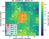 |
Fig. 1 TESS TPF of TOI-756 created with tpfplotter (Aller et al. 2020). The orange pixels define the aperture mask used for extracting the photometry. Additionally, the red circles indicate neighboring objects from the Gaia DR3 catalog, with the circle size corresponding to the brightness difference compared to the target (as indicated in the legend). Our target is marked with a white cross. Pixel scale is 21″/pixel. The co-moving companion of TOI-756 corresponds to the star labeled “2”. |
3.3 Ground-based photometry
The TESS pixel scale is 21″ pixel−1 and photometric apertures typically extend out to roughly 1′, generally causing multiple stars to blend in the TESS aperture. To definitely exclude the presence of another star causing the signal in the TESS data and improve the transit ephemerides, we conducted photometric ground-based follow-up observations in different bands with ExTrA and LCO-CTIO of the field around TOI-756 as part of the TESS Follow-up Observing Program (TFOP)4 Sub Group 1 (Collins 2019).
3.3.1 LCO-CTIO
We used the Las Cumbres Observatory Global Telecope (LCOGT: Brown et al. 2013) 1.0-m network to observe two full transits of TOI-756 b in Sloan-i′ and g′ filters. The telescopes are equipped with 4096 × 4096 SINISTRO Cameras, having an image scale of 0.389″ per pixel and a field of view of 26′ × 26′. The raw data were calibrated by the standard LCOGT BANZAI pipeline (McCully et al. 2018) and photometric measurements were extracted using AstroImageJ (Collins et al. 2017). The two transits were observed at Cerro Tololo Interamerican Observatory (CTIO), the first on 2019 June 12 UT in Sloan-i′ using 4.7" target aperture and the second on July 03, 2019 UT in Sloan-g′ using 5.1" target aperture. The data are shown in Figs. 5 and C.2.
3.3.2 ExTrA
ExTrA (Bonfils et al. 2015) is a near-infrared (0.85–1.55 μm) multi-object spectrophotometer fed by three 60-cm telescopes located at La Silla Observatory in Chile. One full transit (on 2021 February 24) and three partial transits (on March 01, 06, and 27, 2021) of TOI-756 b were observed using two ExTrA telescopes. We used 8″ aperture fibers and the low-resolution mode (R ~ 20) of the spectrophotometer with an exposure time of 60 seconds. Five fiber positioners are used at the focal plane of each telescope to select light from the target and four comparison stars chosen with 2MASS J-band magnitude (Skrutskie et al. 2006) and Gaia effective temperatures (Gaia Collaboration 2018) similar to the target. The resulting ExTrA data were analyzed using a custom data reduction software to produce synthetic photometry in a 0.85–1.55 micron bandpass, described in more detail in Cointepas et al. (2021). The data are shown in Fig. C.3.
3.4 High-resolution imaging
As part of our standard process for validating transiting exoplanets to exclude false positives and to assess the possible contamination of bound or unbound companions on the derived planetary radii (Ciardi et al. 2015), we observed TOI-756 with adaptive optics and speckle imaging at VLT, SOAR, and Gemini.
3.4.1 VLT
TOI-756 was imaged with the NAOS/CONICA instrument on board the Very Large Telescope (NACO/VLT) on the night of July 13, 2019 UT in NGS mode with the Ks filter centered on 2.18 μm (Lenzen et al. 2003; Rousset et al. 2003). We took nine frames with an integration time of 14 s each and dithered between each frame. We performed a standard reduction using a custom IDL pipeline: we subtracted flats and constructed a sky background from the dithered science frames, aligned and co-added the images, and then injected fake companions to determine a 5-σ detection threshold as a function of radius. We obtained a contrast of 4.65 mag at 1″, and no companions were detected. The contrast curve is shown in the top left panel of Fig. B.1.
3.4.2 SOAR
We observed TOI-756 with speckle imaging using the High-Resolution Camera (HRCam) imager on the 4.1 m Southern Astrophysical Research (SOAR) telescope (Tokovinin 2018) on July 14, 2019 UT, observing in Cousins I-band, a similar visible band-pass as TESS. This observation was sensitive to objects fainter by 5.2 at an angular distance of 1 arcsec from the target. More details of the observations within the SOAR TESS survey are available in Ziegler et al. (2020). The 5-σ detection sensitivity and speckle autocorrelation functions from the observation are shown in the top right panel Fig. B.1. No nearby stars were detected within 3″ of TOI-756 in the SOAR observation.
3.4.3 Gemini
TOI-756 was observed on March 12, 2020 and July 05, 2023 UT using the Zorro speckle instrument on Gemini South. Zorro provides speckle imaging in two bands (562 and 832 nm) with output data products including a reconstructed image and robust contrast limits on companion detections (Howell et al. 2011). Both observations provided similar results; TOI-756 has no close companions to within the 5-σ contrast limits obtained (4.84–6.1 magnitudes) at 0.5 arcsec (Fig. B.1, bottom panels).
3.5 Spectroscopic follow-up with combined NIRPS and HARPS
TOI-756 was observed simultaneously from April 4, 2023, to August 23, 2024, with NIRPS (Bouchy et al. 2025) and HARPS (Mayor et al. 2003) echelle spectrographs at the ESO 3.6 m telescope at La Silla Observatory in Chile. NIRPS is a new echelle spectrograph designed for precision radial velocities covering the YJH bands (980–1800 nm). The instrument is equipped with a high-order adaptive optics system and two observing modes: high accuracy (HA; R ~88 000, 0.4″ fiber) and high efficiency (HE; R ~ 75 200, 0.9" fiber), which can be utilized simultaneously with HARPS. TOI-756 was observed as part of the NIRPS-GTO program, under the Follow-up of Transiting Planets subprogram (PID:111.254T.001, 112.25NS.001, 112.25NS.002; PI: Bouchy & Doyon) in HE mode with NIRPS and in EGGS mode (high efficiency mode, R ~ 80 000, 1.4″ fiber) with HARPS. We selected these modes to minimize the modal noise of NIRPS and to maximize the flux by taking the large fibers, especially for HARPS, since the target is relatively faint in the visible (V = 14.6). We also chose to target the sky with fiber B instead of the Fabry-Perot, due to the target’s faintness, to facilitate background light correction. Over 64 individual nights, we collected three spectra of TOI-756 per night with NIRPS (3 exposures of 800 s), which we combined to obtain a median signal-to-noise ratio (S/N) of 28.7 per pixel in the middle of H band. As NIRPS operated alone for seven nights, the HARPS dataset comprise 57 spectra (a single 2400-s exposure per night) with a median S/N of 6.5 per pixel near 550 nm. We choose to take time series of three exposures on NIRPS and then combined them because the maximum recommended exposure time is 900 s on NIRPS due to detector readout noise limitations (Bouchy et al. 2025). We removed the three last HARPS spectra since they were affected by a HARPS shutter problem (24-07-24; 26-07-24; 22-08-24).
For HARPS, we used the extracted spectra from the HARPS-DRS (Lovis & Pepe 2007). For NIRPS, the observations were reduced with both the NIRPS-DRS and APERO. The NIRPS-DRS is based on and adapted from the publicly available ESPRESSO pipeline (Pepe et al. 2021). Several updates have been implemented in the ESPRESSO pipeline to enable the reduction of infrared observations, including a telluric correction following the method of Allart et al. (2022) (see Bouchy et al. 2025). The NIRPS-DRS is the nominal pipeline for NIRPS data reduction for the ESO science archive through the VLT Data Flow System (DFS). APERO (Cook et al. 2022) is the standard data reduction software for the SPIRou near-infrared spectrograph (Donati et al. 2020), and was adapted and made fully compatible with NIRPS. The RV extraction from the reduced data of HARPS and NIRPS was performed with both the cross-correlation method (CCF) and the LBL method of Artigau et al. (2022), available as an open-source package (v0.65.003; LBL5). For the CCF method, we used the CCFs from the HARPS and NIRPS DRS using an M2V and M1V mask respectively. The LBL package is compatible with both NIRPS and HARPS. The method is conceptually similar to template matching (e.g., Anglada-Escudé & Butler 2012; Astudillo-Defru et al. 2017), while being more resilient to outlying spectral features (e.g., telluric residuals, cosmic rays, detector defects) as the template fitting is performed line by line, which facilitates the identification and removal of outliers. For NIRPS, we used the template of a brighter star with a similar spectral type, GL 514 (M1V), from NIRPS-GTO observations. For HARPS, we instead employed the template of GL 699 (M4V) from public data obtained via the ESO archive (Delmotte et al. 2006). An additional telluric correction was performed for HARPS inside the LBL code by fitting a TAPAS atmospheric model (Bertaux et al. 2014).
Finally, for the analysis presented in Sect. 5.2, we used the HARPS data processed using the DRS pipeline in combination with LBL, and the NIRPS data reduced with APERO, which provides a slightly better telluric absorption correction, also in conjunction with LBL. We employed nightly binned data and applied a preprocessing step to exclude points with higher uncertainties than the majority, using a 95% percentile error-based filtering on RVs and the second-order derivative D2V indicator, defined in Artigau et al. (2022). Variations in the second-order derivative can be associated with changes in the FWHM from the CCF method. All the data will be publicly available through the DACE platform6 after publication.
4 Stellar characterization
4.1 Spectroscopic parameters
The derivation of spectroscopic stellar parameters was done by applying different techniques to the HARPS and NIRPS spectra. For the first technique, we combined all the individual HARPS spectra with the task scombine within IRAF7 to obtain a high S/N spectrum. We used the machine learning tool ODUSSEAS8 (Antoniadis-Karnavas et al. 2020, 2024) to derive the effective temperature (Teff) and metallicity ([Fe/H]). This tool measures the pseudo equivalent widths (EWs) of a set of ~4000 lines in the optical spectra. Then, it applies a machine learning model trained with the same lines measured and calibrated in a reference sample of 65 M dwarfs observed with HARPS for which their [Fe/H] were obtained from photometric calibrations (Neves et al. 2012) and their Teff from interferometric calibrations (Khata et al. 2021). With this method, we derived a Teff = 3620±94 K and [Fe/H] = 0.14±0.11 dex.
For the second technique, the combined telluric-corrected NIRPS spectrum obtained with APERO is used to determine the stellar parameters and abundances. Following the methodology of Jahandar et al. (2024, 2025), initially developed for SPIRou spectra (Donati et al. 2020), we retrieve the effective temperature Teff, overall metallicity [M/H] and chemical abundances of TOI-756. We first determine Teff and [M/H] by fitting individual spectral lines to a grid of PHOENIX ACES stellar models (Husser et al. 2013) convolved to the resolution of NIRPS. The models are interpolated to fixed log g = 4.75 based on the value obtained in Sect. 4.2. We find Teff = 3710 ± 33 K and [M/H] = 0.17 ± 0.08 dex. While Teff is in agreement with the value derived from HARPS, we observe a significant discrepancy between the measurements of the different bands, obtaining 3575 ± 23 K for Y and J, and 3803 ± 17 K for H. This discrepancy could be due to the lack of K-band coverage in NIRPS, as this spectral range was found to be crucial in the determination of Teff with SPIRou (Jahandar et al. 2024). To better reflect the bimodality of the distribution, we inflated the uncertainty on the temperature to the half-distance of the two chromatic measurements (Teff = 3710 ± 113 K). The temperatures obtained for NIRPS and HARPS were then combined with a weighted average to give the adopted effective temperature, Teff = 3657 ± 72 K. However, for the abundance analysis, we used the effective temperature obtained from HARPS to be more conservative.
The abundances of chemical species are determined by fitting the PHOENIX grid to individual spectral lines (Jahandar et al. 2024, 2025) with fixed Teff of 3620 K. The stellar abundances measured from the NIRPS spectrum are recorded in Table 2, although it should be noted that the assumption of a fixed Teff likely results in an underestimation of the uncertainties.
TOI-756 stellar abundances measured with NIRPS.
4.2 Mass, radius, and age
To derive the mass and radius of the star, we constructed the spectral energy distribution (SED) using the flux densities from the photometric bands GBP, G, and GRP from the Gaia mission (Gaia Collaboration 2018), B and V from APASS (Henden et al. 2015), J, H, and Ks from the 2MASS project (Skrutskie et al. 2006), and W1, W2, W3, and W4 from the WISE mission (Wright et al. 2010). For the SED modeling process, we employed the Virtual Observatory Spectral Analyzer (VOSA) tool (Bayo et al. 2008). Theoretical models such as BTSettl (Allard et al. 2012), Kurucz (Kurucz 1993), and Castelli & Kurucz (Castelli & Kurucz 2003) are used to construct the synthetic SEDs, where the most suited model was BT Settl with Teff = 3600 K, [M/H] = 0 dex, and log(g) = 4.5 cm s−2. VOSA uses a χ2 minimization technique to achieve the best fit between the theoretical curve and the observational data, taking into account the observed flux, the theoretical flux predicted by the model, the observational error related to the flux, the number of photometric points, input parameters, the object’s radius, and the distance between the observer and the object. The resulting analysis is shown in Fig. 2.
We then integrated the observed SED to obtain the bolometric luminosity: L⋆ = 0.03805 ± 0.00011 L⊙. We obtained the stellar radius R⋆ = 0.501 ± 0.014 R⊙ using the Stefan-Boltzmann law, ![Mathematical equation: $\[L_{\star}=4 \pi R \sigma T_{\text {eff }}^{4}\]$](/articles/aa/full_html/2025/10/aa55684-25/aa55684-25-eq5.png) . Finally, the stellar mass (M⋆ = 0.505 ± 0.019 M⊙) was estimated using Equation 6 from Schweitzer et al. (2019).
. Finally, the stellar mass (M⋆ = 0.505 ± 0.019 M⊙) was estimated using Equation 6 from Schweitzer et al. (2019).
We independently derived the mass and radius of TOI-756 using the empirically established M-dwarf mass-luminosity and radius-luminosity relations from Mann et al. (2019) and Mann et al. (2015), respectively. To do this, we utilized the Gaia stellar parallax and the Ks magnitude from 2MASS to calculate the absolute Ks magnitude (MK). We employed a Monte Carlo method to propagate the uncertainties and incorporated the intrinsic errors of the relations, which are 2.89% for the radius and 2.2% for the mass, into our results.
The results of these two independent methods are compiled in Table 3. The two methods give very consistent radius and mass values. We combined the resulting stellar masses and radii, taking the larger uncertainties to be conservative, as final stellar parameters. Together with the results of Sect. 4.1, we derived the associated stellar luminosity (L*), gravity (log g*), and density (ρ*). These final parameters are listed in Table 1.
Additionally, to estimate the age of the star, we used the code isoAR9 from Brahm et al. (2018) using the Teff and [Fe/H] derived in Sect. 4.1, plus Gaia photometry and parsec isochrones. The resulting age of ![Mathematical equation: $\[3.2_{-2.3}^{+5.5}\]$](/articles/aa/full_html/2025/10/aa55684-25/aa55684-25-eq10.png) Gyr is poorly constrained, which is expected for an M dwarf.
Gyr is poorly constrained, which is expected for an M dwarf.
Finally, space velocities ULSR, VLSR, and WLSR10, were calculated using positions, parallaxes, proper motions, and RVs from Gaia DR3. To relate the space velocities to the local standard of rest (LSR), the Sun’s velocity components relative to the LSR (U⊙, V⊙, W⊙) = (11.10, 12.24, 7.25) km s−1 from Schönrich et al. (2010) were added. We obtained: ULSR = −57.56 ± 0.64 km s−1, VLSR = −44.82 ± 0.97 km s−1 and WLSR = 22.18 ± 0.36 km s−1. According to the probabilistic approach of Bensby et al. (2014), the galactic kinematic indicates that TOI-756 is a thin disc population star. All the adopted astrometric and photometric stellar properties of TOI-756 are listed in Table 1. According to all these parameters and the Table 5 from Pecaut & Mamajek (2013), TOI-756 corresponds well to a M1V star.
In terms of stellar activity, TOI-756 appears to be rather quiet, with no identifiable rotation period. Inspecting the TESS SAP light curves and ASAS (Pojmanski 1997) data with Lomb–Scargle periodograms reveal no significant peaks. Similarly, no notable signals are observed in the RV indicators from HARPS and NIRPS. Additionally, we used the HARPS DRS data to compute the logR′hk from the S-index measuring Ca H and K emission. We used the relations from Suárez Mascareño et al. (2015, 2016), and found a median value of −5.16, in line with the absence of activity of the star.
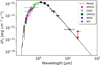 |
Fig. 2 SED of TOI-756, constructed using broadband photometric data from APASS (magenta), Gaia (green), 2MASS (black), and WISE (blue). The upper limit for the WISE W4 band is indicated by a red dot. The horizontal error bars represent the passband widths of the respective filters. Below the SED, the residuals are shown, normalized to the photometric errors. The SED was modeled using the BT Settl atmospheric model (Allard et al. 2012) with Teff = 3600 K, [M/H] = 0 dex, and log g⋆ = 4.5 cm s−2. |
TOI-756 stellar parameters derived by different methods.
5 Photometric and radial velocity analysis
We utilized the software package juliet (Espinoza et al. 2019) to model both the photometric and RV data. This algorithm integrates several publicly available tools for modeling transits (batman; Kreidberg 2015), RVs (radvel; Fulton et al. 2018), and Gaussian processes (GPs; george; Ambikasaran et al. 2015; celerite, Foreman-Mackey et al. 2017). To compare different models, juliet efficiently calculates the Bayesian evidence (ln Z) using dynesty (Speagle 2020), a Python package that estimates Bayesian posteriors and evidence through nested sampling methods. Unlike traditional approaches that begin with an initial parameter vector centered around a likelihood maximum found via optimization, nested sampling algorithms draw samples directly from the priors. Throughout our analyses, we ensured that we had a sufficient number of live points Nlive relative to the number of free parameters d (Nlive ≥ 25 × d), preventing us from missing peaks in the parameter space. We conducted several analyses: starting with only the photometry, and using the resulting planet parameters as priors for a subsequent RV analysis and then a joint fit of the two.
5.1 Photometry analysis
First, we used juliet to model the photometry. We used the TESS PDCSAP fluxes of the four sectors where our planet candidate was initially detected, the two transits from LCO-CTIO telescope in i′ and g′ bands and the four transits from ExTrA telescopes. The transit model fits the stellar density ρ⋆ along with the planetary and jitter parameters. We adopted a few parametrization modifications when dealing with the transit photometry. Rather than fitting directly for the planet-to-star radius ratio (p = Rp/R⋆) and the impact parameter of the orbit (b = a/R⋆cosi), juliet uses the parametrization introduced in Espinoza (2018) and fits for the parameters r1 and r2 to guarantee full exploration of physically plausible values in the (p,b) plane. Additionally, we implemented a “power-2” limb-darkening law in juliet, as shown to be the best for fitting cold star intensity profiles (Morello et al. 2017). We derived the “power-2” stellar limb-darkening coefficients and their uncertainties for each photometric filter used using the LDCU11 code (Deline et al. 2022). The LDCU code is a modified version of the Python routine implemented by Espinoza & Jordán (2015) that computes the limb-darkening coefficients and their corresponding uncertainties using a set of stellar intensity profiles accounting for the uncertainties on the stellar parameters. The stellar intensity profiles are generated based on two libraries of synthetic stellar spectra: ATLAS (Kurucz 1979) and PHOENIX (Husser et al. 2013). We utilized the limb-darkening coefficients determined from LDCU as Gaussian priors for the fit. Since the TESS PDCSAP light curves are already corrected for contamination, we fixed the TESS dilution factor to one. We applied the same assumption to the ground-based photometry, as the apertures are free from contaminating sources. We added in quadrature jitter terms σi to all the photometric uncertainties, which may be underestimated due to additional systematics. To account for the remaining photometric variability, we included a GP for Sectors 10 and 11 of TESS PDCSAP fluxes using a Matérn 3/2 kernel with hyper-parameters amplitude (σGP) and timescale (ρGP). Including GPs for Sectors 37 and 64 led to negligible amplitudes, so we did not apply the GP correction to these sectors. We detrended the LCO-CTIO transit in the g′ band with airmass and the ExTrA data was detrended with a GP using a Matérn 3/2 kernel as suggested by Cointepas et al. (2021). The resulting detrending can be seen in Appendix C.
We first assumed a circular orbit so we fixed the eccentricity to zero and used normal priors around the ExoFOP values for the period and transit epoch. We used a normal prior for stellar density using the value derived in Sect. 4. In the first instance, we fit the TESS photometry alone to constrain these parameters and then used the resulting posteriors to jointly fit all the photometry (see Appendix C). We first used the classical (p,b) parametrization to let the planet-to-star ratio p to be different among photometric filters to check for possible false positives. We found consistent transit depths among the different photometric bands: pTESS = 0.050 ± 0.001, pLCO–i′ = 0.052 ± 0.003, pLCO–g′ = 0.048 ± 0.004 and pExTrA = 0.051 ± 0.005. We then fitted only one set of r1 and r2 parameters for the planet. For the joint photometry fit, we only took TESS data around the transits (± 3 hours around the transit times calculated with the resulting period and transit epoch of the TESS-only fit) in order to reduce the fit time of the joint analysis with juliet.
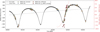 |
Fig. 3 RV data from HARPS (blue dots) and NIRPS measurements. The NIRPS data is separated in unaffected datapoints (orange dots) and affected datapoints (red triangles) by the crossing of the Vsyst and BERV velocities during the observations. Yellow dots are NIRPS data with the correction explained in Sect. 5.2.2. The dotted red line together with the right y axis represent the total velocity of TOI-756, showing the crossing of the BERV with the Vsyst. The complete inferred model in Sect. 5.2.3, which comprises signals from the two planets along with the linear model for the acceleration (in gray), is represented by a black solid line. |
5.2 Radial velocity analysis
The reduction and preprocessing of the RVs are explained in Sect. 3.5 and the resulting datasets are shown in Fig. 3. A significant RV variation was detected for TOI-756, suggesting the presence of an additional companion to the TESS sub-Neptune. Several possible orbital periods were initially explored, motivating further observations to constrain this signal alongside that of the 1.24-day sub-Neptune. These efforts led to the confirmation of an eccentric companion on a ~150-day orbit. In addition, the RVs reveal an acceleration, hinting at a third, more distant object.
5.2.1 Telluric contamination of the NIR data during the Vsyst−BERV crossing
One of the main challenges of NIRPS and near-infrared spectroscopy is the contamination of the stellar spectrum by molecular species in Earth’s atmosphere. This issue is particularly pronounced when observing M dwarfs, whose spectra also contain absorption features from species such as H2O and CH4. The NIRPS-DRS includes a telluric absorption correction based on Allart et al. (2022), but the observed spectra of faint M dwarfs are further dominated by strong emission lines from Earth’s atmosphere, notably from OH. These emission lines are typically corrected during the reduction process (Srivastava et al. in prep), but their non-LTE nature makes them more challenging to correct, as they cannot be modeled using standard telluric line approaches.
However, this contamination becomes especially problematic when aiming to measure precise stellar radial velocities, particularly when telluric lines coincide with the absorption lines of the star. This situation arises when the barycentric Earth radial velocity (BERV) crosses the systemic velocity (Vsyst) of the observed star. In such cases, the correction is challenging, as blending between the stellar and telluric lines distorts the stellar line profiles, leading to erroneous RV estimates. Since the telluric emission features are more numerous and stronger in H compared to the J, there will be a chromatic offset induced in the calculated RVs between the “red” wavelengths, and “blue” wavelengths.
We observed this phenomenon between RJD = 60 365 and 60 416, when the Keplerian fit of the outer companion of TOI-756 showed clear outliers of ~100–200 m s−1 in the NIRPS RVs (see top panel of Fig. 4). This effect is illustrated in Fig. 3, the NIRPS data is represented as red triangles when the absolute total velocity |Vtot| = |Vsyst − BERV| ≤ 10 km s−1, corresponding to approximately twice the typical spectra line FWHM for slow rotating M dwarfs (5 km s−1). The HARPS data are shown using blue dots and the non-affected NIRPS data (Vtot > 10 km s−1) using orange dots. In this Figure 3, we plotted the relative velocity to the systemic velocity of TOI-756, which was found to be Vsyst ~ 15.2 km s−1. This phenomenon also induces distortions in the stellar line profiles, which are evident in the systemic variations of different LBL indicators, such as D2V and ΔT (Artigau et al. 2024), as shown in Fig. 4.
 |
Fig. 4 NIRPS data residuals (upper panel) and LBL indicators D2V (middle panel), along with dTemp (ΔT) calculated at 3500 K close to the effective temperature of TOI-756 (bottom panel). Orange dots are the indicators from unaffected NIRPS data, red triangles are the affected spectra by Vsyst−BERV crossing and yellow dots are the indicators with the correction explained in Sect. 5.2.2. |
5.2.2 Correction with removing affected lines in the LBL
The advantage of using the line-by-line (LBL) technique to derive radial velocities and other spectral indicators lies in its ability to provide individual measurements for each spectral line across the entire spectrum. The observed discrepancy, where NIRPS RVs appear underestimated and then overestimated relative to the RV fit, is caused by the crossing of stellar absorption lines with atmospheric OH emission lines, primarily arising from excitation of rotational-vibrational modes of the OH molecule.
To mitigate this effect, we utilized the HITRAN12 database (Gordon et al. 2022) to identify OH lines present within the NIRPS spectral range. We selected the 25% most intense OH lines and removed the LBL-derived measurements in a ±20 km s−1 window around these lines, accounting for the approximate width of both OH and stellar lines (~10 km s−1 each). This process reduced the number of spectral lines used in the LBL analysis from 26 301 to 17 253, inevitably increasing the RV uncertainties. We then recomputed the final radial velocity and indicator values for each epoch using the same LBL method, which robustly averages the per-line values while down-weighting outliers (Appendix B of Artigau et al. 2022). We applied this correction for all the NIRPS data for consistency. The corrected data are displayed as yellow dots in Figures 3 and 4.
This correction successfully brought NIRPS RVs into agreement with HARPS and effectively removed the systematic distortions previously visible in the residuals of the Keplerian fit and in the spectral indicators (Fig. 4). The corrected indicators now show consistent values across epochs, with no residual systematics during the Vsys–BERV crossing. Additionally, the root mean square (RMS) of the residuals and the indicators, displayed in the same figure, demonstrates a significant decrease after correction.
We applied the same technique to the mask used to derived the NIRPS DRS cross-correlation function (CCF) data, using the OH line list from the DRS telluric correction module. While this also mitigated the effect, the CCF method relies on significantly fewer spectral lines than the LBL approach, leading to much larger error bars after correction. Consequently, we opted to retain the LBL-derived values for our analysis.
5.2.3 Radial velocity analysis and joint modeling with juliet
juliet was also used to model these RV datasets. We used a two-planet plus a linear trend model. At first, we fixed the eccentricity of the TESS planet TOI-756 b to zero. We accounted for the evident eccentricity of the outer companion by fitting for the parameters ![Mathematical equation: $\[\sqrt{e} cos (\omega), \sqrt{e} sin (\omega)\]$](/articles/aa/full_html/2025/10/aa55684-25/aa55684-25-eq11.png) , as implemented in juliet. This parametrization has been shown to improve the exploration of the eccentricity–argument of periastron parameter space (Lucy & Sweeney 1971). We used the period and transit epoch results of TOI-756 b of the photometry fit (Sect. 5.1) as priors for the RV fits.
, as implemented in juliet. This parametrization has been shown to improve the exploration of the eccentricity–argument of periastron parameter space (Lucy & Sweeney 1971). We used the period and transit epoch results of TOI-756 b of the photometry fit (Sect. 5.1) as priors for the RV fits.
We compared several analyses: (1) NIRPS data corrected using the method described in Sect. 5.2.2 combined with HARPS data; (2) uncorrected NIRPS data with the affected points removed, also combined with HARPS data; (3) HARPS data only; and (4) corrected NIRPS data only. We present the posteriors of the main changing planetary parameters of the different fits in Table 4. We did not put the period and transit epoch of planet b in this table because they are very similar for these analyses since they are highly constrained by the photometry fit priors. The resulting parameters exhibit good consistency within 1σ for all our different analyses.
Since the NIRPS corrected data combined with the HARPS data are fully consistent with the other fits and included all RV points, we choose this dataset as the final one. We do a joint fit of the RVs and photometry with juliet: NIRPS corrected RVs, HARPS RVs, TESS, LCO-CTIO and ExTrA. In order to prevent any potential Lucy-Sweeney bias in the eccentricity measurement (Lucy & Sweeney 1971; Hara et al. 2019), we fixed the orbital eccentricity of the planet b to zero. However, to explore the possibility of non-circular orbit, we ran a separate analysis without any constraints on the eccentricity. The logarithmic evidence for the eccentric model is lower than for the circular one (55 557 vs. 55 580), and the fitted jitter values for both HARPS and NIRPS RVs are higher in the eccentric case, further supporting the preference for the circular model. The fitted eccentricity for TOI-756 b is eb = ![Mathematical equation: $\[0.096_{-0.067}^{+0.092}\]$](/articles/aa/full_html/2025/10/aa55684-25/aa55684-25-eq12.png) . Therefore, the condition e > 2.45 σe (Lucy & Sweeney 1971) is not satisfied, which suggests that the RV data are compatible with a circular orbit. For now, the current data do not provide sufficient precision to draw a firm conclusion regarding the orbital eccentricity. Additionally, in Table 5, we show that the 3-σ upper limit on the eccentricity for TOI-756 b is 0.51. The fitted and derived parameters for TOI-756 b and TOI-756 c are presented in Table 5.
. Therefore, the condition e > 2.45 σe (Lucy & Sweeney 1971) is not satisfied, which suggests that the RV data are compatible with a circular orbit. For now, the current data do not provide sufficient precision to draw a firm conclusion regarding the orbital eccentricity. Additionally, in Table 5, we show that the 3-σ upper limit on the eccentricity for TOI-756 b is 0.51. The fitted and derived parameters for TOI-756 b and TOI-756 c are presented in Table 5.
The priors and posteriors of the joint fit can be found in Table C.2. Fig. 5 shows the phase-folded light-curves of the photometry fit. Fig. 3 shows RV data together with the resulting model from the joint fit and Fig. 6 the phase-folded RV curves for the two planets.
We searched for a possible transit of planet c in the TESS data by phase-folding the light curve using its orbital period and time of conjunction. Although TESS observations cover the expected transit window, no transit signal is visible in the data, allowing us to exclude a transiting configuration. Furthermore, assuming coplanar orbits aligned with the inclination of TOI 756 b (85.5°), we estimated the expected impact parameter of the outer planet based on its semi-major axis and the stellar radius. We obtained bc = 14.3 ± 0.7, a value well above 1.
Posterior planetary parameters of the different RV fits.
Fitted and derived parameters for TOI-756 b and TOI-756 c.
6 Discussion
We present the discovery and characterization of the transiting sub-Neptune TOI-756 b and the non-transiting eccentric cold giant TOI-756 c, both orbiting the M1V star TOI-756. TOI-756 b has an orbital period of 1.24 days, a radius of 2.81 ± 0.10 R⊕ and a mass of 9.8 ± 1.7 M⊕. The outer companion, TOI-756c, follows an eccentric (0.45) 149-day orbit and has a minimum mass of 4.05 ± 0.11 MJup. Using the stellar parameters (Table 1), we determine the semi-major axes of TOI-756 b and TOI-756 c to be 0.0180 ± 0.0002 au and 0.439 ± 0.005 au, respectively. Assuming zero albedo and full heat redistribution, the equilibrium temperature of TOI-756 b is 934 ± 24 K, with a stellar insolation of 127 ± 13 S⊕. For TOI-756c, we estimate an equilibrium temperature of 194 ± 5 K and a stellar insolation of 0.24 ± 0.02 S⊕ averaged along the eccentric orbit. In addition, the RVs present an acceleration of 145.6 ± 5.2 m s−1 yr−1 hinting at an additional component in the system.
6.1 NIRPS + HARPS performances
The characterization of this system was made possible by TESS and ground-based facilities for the photometric analysis of the inner transiting planet, as well as by the combination of HARPS and NIRPS for RV follow-up. The synergy between these two spectrographs enabled us to precisely characterize an early-M with a peculiar planetary-system configuration. The benefit of this combination is evident in Table 4: using HARPS (NIRPS) alone, the semi-amplitude of TOI-756 b is determined with a precision of 31% (42%), whereas combining HARPS and NIRPS improves this to 17% in the joint RV and photometry fit. All other fitted parameters also benefit from improved precision thanks to this joint analysis. This study highlights the added value of NIRPS (to HARPS) in characterizing a low-mass planet around a faint M dwarf (V = 14.6, J = 11.1), compared to typical radial velocity targets. Independently, the two instruments have similar median photon noises. The median photon noise is 5.5 m s−1 for HARPS and 15.4 m s−1 for NIRPS, but the latter having increased from 8.4 m s−1 due to the removal of affected lines during the LBL computation (see Sect. 5.2.2). The fitted jitter values for both instruments are similar, around 15 m s−1, which matches the photon noise for NIRPS but is elevated compared to HARPS photon noise. This suggests the presence of atmospheric residuals or enhanced stellar activity in the optical range. Given the low S/N regime in which HARPS is operating, increased background sky contamination and possible interference from the Moon are to be expected. At such low S/N, the LBL method is also likely to underestimate the uncertainties associated with the derived RVs.
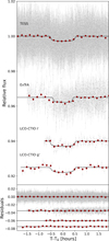 |
Fig. 5 Top panel: phase-folded TESS, ExTrA, and LCO-CTIO light curves of TOI-756 b (gray points). Dark red circles are data binned to 10 min. The black lines represent the median model of each instrument from the joint fit. Bottom panel: residuals of the data compared to the model. An arbitrary offset has been added to the ground-based photometry for clarity. |
6.2 TOI-756 b: Internal structure, composition, and population context
6.2.1 A volatile-rich sub-Neptune around an M dwarf
The characterization of TOI-756 b adds to the currently small population of known transiting sub-Neptunes (2 R⊕ < Rp < 4 R⊕) around M dwarfs, as shown in the Mass-Radius (M-R) diagram (Fig. 7) where the red (gray) dots represent planets from the PlanetS catalog (Parc et al. 2024; Otegi et al. 2020) orbiting M dwarfs (FGK dwarfs). Inside this population, Parc et al. (2024) identified statistical evidence for small sub-Neptunes (1.8 R⊕ < Rp < 2.8 R⊕) being less dense around M dwarfs than around FGK dwarfs with a p-value of 0.013, rejecting the null hypothesis. This means that the densities of small sub-Neptunes orbiting M and FGK dwarfs belong to different distributions. We updated this analysis with the up-to-date PlanetS catalog and by including TOI-756 b, which had a density of 2.42 g cm−3. We choose to increase the upper radius limit of this sample to 2.9 R⊕ (2.8 R⊕ having been chosen to capture all small sub-Neptunes around M dwarfs at that time). We find, with the same Mann-Whitney U test (Wilcoxon 1945; Mann & Whitney 1947), an improved pvalue of 0.006 for this trend. However, these two analysis are not taking into account the uncertainties on the density measurements. We did a Mann–Whitney U test on 10 000 samples using a bootstrapping method to draw density values in the density distributions of each planet and obtained a median p-value of 0.015, a still significant value. However, the sample remains small and the increase of the well-characterized planets in this parameter space is one of the objectives of the NIRPS GTO SP2 subprogram “sub-Neptunes” described in Sect. 2.
We plot the mass and radius of TOI-756 b, alongside with the small planets of the PlanetS catalog in Fig. 7. With its density of 2.42 g cm−3 (and looking at the composition lines shown in the same figure), TOI-756 b lies above the 50% water plus Earth-composition line at 1000 K (at 2σ) from Aguichine et al. (2021) (dark blue dotted line). A pure silicate interior with a 50% steam atmosphere can explain within 1σ the radius and mass of TOI-756 b for this model (light blue dotted line). Furthermore, it corresponds well within 1σ to the Earth-composition with a H2/He dominated-atmosphere of 1% the mass from Zeng et al. (2019) (pink dotted line). As models from Aguichine et al. (2021) include pure steam atmosphere with no solubility between the atmosphere and the mantle+core compared to Luo et al. (2024) models (e.g., green dotted line), and are static in time (compared to Aguichine et al. 2025), they can be considered to over-estimate the radii of the planets. They can thus be interpreted as an upper limit of M-R composition lines for water-rich models. In addition, due to its high equilibrium temperature of approximately 934 K, any water present in the atmosphere of TOI-756 b is expected to be in a supercritical state. In conclusion, it is more likely that TOI-756 b needs an amount of hydrogen/helium in its atmosphere to explain its density, in the form of pure H/He envelope or mixed supercritical H2O and H/He. This places the planet within the “miscible-envelope sub-Neptunes” category defined by Benneke et al. (2024). Atmospheric characterization could confirm this classification by revealing a mean molecular weight significantly higher than that of Jupiter (2.2) or Neptune (2.53–2.69). We investigate this in greater detail in the following section.
Interestingly, Schlecker et al. (2021) found a difference in the bulk composition of inner small planets with and without cold Jupiters. High-density small planets point to the existence of outer giant planets in the same system. Conversely, a present cold Jupiter gives rise to rocky, volatile-depleted inner super-Earths, by obstructing inward migration of icy planets that form on distant orbits. However, TOI-756 c lies beyond the system’s ice line, and its formation may have contributed to the inward delivery of water-rich material, as proposed for the Solar System by Raymond & Izidoro (2017). This process could account for the potentially ice-rich composition of TOI-756 b. As shown by Bitsch et al. (2021), the water content of an inner sub-Neptune can provide valuable insights into the formation location and timescale of an outer giant planet relative to the water ice line, offering constraints on planet formation theories.
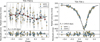 |
Fig. 6 Phase-folded RVs with the resulting model and its residuals for TOI-756 b (left) and TOI-756 c (right). In red dots, binned data combining HARPS (blue dots) and NIRPS (yellow dots). The error-bars in light gray account for the fitted jitters. |
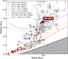 |
Fig. 7 Mass-radius diagram of small exoplanets (with radii ranging from 1–4 R⊕) with precise densities from the PlanetS catalog. The red (gray) dots correspond to exoplanets orbiting M dwarfs (FGK dwarfs). The composition lines of pure silicates (yellow dashed), Earth-like planets (red dashed), and pure iron (solid black) from Zeng et al. (2016, 2019) are displayed. The red hexagon represent TOI-756 b. Two compositions line that incorporate both water and terrestrial elements from Aguichine et al. (2021) models, matching the equilibrium temperature of the planet, are plotted as light and dark blue dotted lines. Two compositions of Earth with an hydrogen-rich atmospheres from Zeng et al. (2019) are represented in pink and purple dotted lines. This plot has been generated with mr-plotter (https://github.com/castro-gzlz/mr-plotter/). |
6.2.2 Detailed interior modeling
We perform a detailed interior characterization of TOI-756 b using a Bayesian inference approach, adopting the emcee affineinvariant ensemble sampler (Foreman-Mackey et al. 2013) coupled to a three-layer interior structure model. The planetary interior is assumed to be composed of an Fe-Ni metallic core and a silicate mantle (SUPEREARTH Valencia et al. 2007), while the outermost layer consists of either a hydrogen-helium envelope or a water vapor atmosphere modeled using the CEPAM code (Guillot & Morel 1995), with equations of state from Saumon et al. (1995) for H/He and French et al. (2009) for H2O. In all cases, we assume that the rocky interior contains no volatiles and follow the numerical set-up given in Plotnykov & Valencia (2020).
To explore the range of possible atmospheric mass fraction (AMF) values, we consider two sub-Neptune composition scenarios: (1) the planet has a H/He envelope (75% of H2 to 25% He) and (2) the planet has pure H2O envelope. For these scenarios, we impose stellar-informed priors on the rocky interior based on the host star’s refractory abundances taken from Table 2, namely,
![Mathematical equation: $\[\mathrm{Fe} / \mathrm{Mg}_{\text {planet }} \sim \mathcal{N}\left(\mathrm{Fe} / \mathrm{Mg}_{\text {star }}, \sigma_{\text {star }}^2\right); \mathrm{Fe} / \mathrm{Si}_{\text {planet }} \sim \mathcal{N}\left(\mathrm{Fe} / \mathrm{Si}_{\text {star }}, \sigma_{\text {star }}^2\right),\]$](/articles/aa/full_html/2025/10/aa55684-25/aa55684-25-eq42.png)
where all ratios are by weight. Additionally, the mantle mineralogy is allowed to vary in terms of the Bridgmanite to Wustite ratio (MgSiO3 vs MgO, xWu). These assumptions effectively constrain the rocky core-mass fraction (![Mathematical equation: $\[\mathrm{CMF}=\frac{\mathrm{rcmf}}{\mathrm{rcmf}+1}\]$](/articles/aa/full_html/2025/10/aa55684-25/aa55684-25-eq43.png) , where rcmf is the core to mantle mass ratio, Mcore/Mmantle) of the planet and mitigate problem of compositional degeneracy.
, where rcmf is the core to mantle mass ratio, Mcore/Mmantle) of the planet and mitigate problem of compositional degeneracy.
Considering case (1) where TOI-756 b has retained its primordial H/He envelope, we recover a well-constrained AMF = 0.023 ± 0.003 (3 wt%), with a corresponding CMF = 0.27 ± 0.03. Note that this strong constraint may partly result from underestimated abundance uncertainties, as the values were derived assuming a fixed Teff (see Sect. 4.2). However, if we impose no prior on the rocky composition, the envelope has an AMF = 0.03 ± 0.01 (3 wt%), while the interior has almost a uniform distribution of CMF = 0.5 ± 0.3. These results suggesting strong evidence that this planet has a volatile envelope based on mass-radius data alone. For the case where the envelope is composed of pure water vapor (2), we find that AMF = 0.79 ± 0.10 and CMF = 0.27 ± 0.03. This very high value of AMF of pure water vapor is highly unlikely when linked to formation theories. Our analysis suggests that the presence of H/He in the atmosphere is more plausible, although a combination of both scenarios (1) and (2) remains a possibility. Regardless, this confirms that TOI-756 b requires a volatile envelope to account for its density, and that the abundances derived from NIRPS spectra have allowed us to better constrain both the CMF and AMF in the case of a pure H/He envelope. The resulting corner plots of this analysis are shown Fig. D.1.
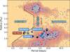 |
Fig. 8 Planet radius as a function of orbital period for known exoplanets from NASA Exoplanet Archive with a radius precision below 8%. We highlighted the Neptunian desert, ridge, and savanna regions from Castro-González et al. (2024). The colorcode represents the observed density of planets. TOI-756 b is depicted as a dark red hexagon. Light blue symbols represent sub-Neptunes in systems hosting eccentric giant companions: crosses indicate systems with only giant planets, while circles correspond to systems containing both small and giant planets. In contrast, dark blue circles represent sub-Neptunes in systems with non-eccentric giant planets. The description of the selection is made in Sect. 6.3.1. This plot has been generated with nep-des (https://github.com/castro-gzlz/nep-des/). |
6.2.3 A planet at the radius cliff and in the Neptune desert
TOI-756 b is a very interesting target in this sample of small sub-Neptunes around M dwarfs. Indeed, it is a unique object close to the “radius cliff”, a steep drop in planet occurrence between 2.5 and 4.0 R⊕ (Borucki et al. 2011; Howard et al. 2012; Fulton et al. 2017). This still poorly explored demographic feature seems to vary in location with the host star’s spectral type as also seen with the radius valley (Ho et al. 2024; Parc et al. 2024; Burn et al. 2024). Kite et al. (2019) proposed that atmospheric sequestration into magma could explain this phenomenon, as larger atmospheres reach the critical base pressure needed for H2 to dissolve into the core. Ongoing studies seek to understand variations in atmospheric observables across these features to better comprehend their underlying physics.
Moreover, TOI-756 b lies at the very lower edge of the Neptune desert. We plotted its location together with the boundaries of the desert as defined in Castro-González et al. (2024) in Fig. 8. The main hy pothesis for the shaping of the lower edge of the Neptune desert is through hydrodynamical atmospheric escape, driven by intense stellar X-ray and extreme ultraviolet (XUV) irradiation (e.g., Yelle 2004; Tian et al. 2005; Owen & Jackson 2012; McDonald et al. 2019). This process can strip the gaseous envelopes of close-in Neptune-sized planets, leaving behind smaller, denser remnants such as sub-Neptunes or bare rocky cores (Lopez & Fortney 2013). Therefore, TOI-756 b may have lost at least part of its gaseous envelope as a result of prolonged exposure to XUV irradiation from its host star. Notably, M dwarfs remain active for significantly longer periods than Sun-like stars (Ribas et al. 2005), extending the timescale over which atmospheric escape operate. Additionally, the possible non-zero eccentricity of the sub-Neptune, along with the eccentricity of TOI-756 c and the presence of a third body, may suggest dynamical activity, potentially involving high-eccentricity tidal migration (HEM). HEM, which includes mechanisms such as planet-planet scattering (e.g., Gratia & Fabrycky 2017), Kozai–Lidov migration (e.g., Wu & Murray 2003), and secular chaos (e.g., Wu & Lithwick 2011), can occur at any stage after disk dispersal, from early evolutionary phases to several billion years later. HEM typically leads to strongly misaligned orbits, erasing any memory of the system’s primordial configuration. In this scenario, a distant massive companion excites the eccentricity of the inner planet via gravitational perturbations, which is then followed by tidal circularization and inward migration due to energy dissipation induced by stellar tides (e.g., Rasio & Ford 1996). This process can be investigated by measuring the spin–orbit alignment of the transiting planet using Rossiter–McLaughlin (RM) observations (Rossiter 1924; McLaughlin 1924). These dynamical processes are considered to be key factors in shaping the Neptune desert. Additionally, the boundaries of the Neptune desert may vary with the spectral type of the host star, and to date, there has been no comprehensive study of the Neptune desert around M dwarfs. Indeed, for a given orbital period, a planet orbiting an M dwarf receives intuitively less stellar flux than planets around other types of stars, which could affect the atmospheric escape kick off. Interestingly, TOI-756 b does not show the high density commonly found in planets within the Neptune desert, such as TOI-849 b (Armstrong et al. 2020). Its ability to retain an atmosphere despite strong irradiation could be explained by its orbit around a metal-rich star, since metal-rich atmospheres are thought to be more resistant to photoevaporative mass loss (Owen & Murray-Clay 2018; Wilson et al. 2022).
Atmospheric characterization of planets located within the radius cliff and Neptune desert could help test theories regarding the origins of these demographic features. With a Transmission Spectroscopic Metric (TSM) of 63 (Kempton et al. 2018), TOI-756 b stands out as a promising target for future transmission spectroscopy studies, for instance with JWST (Gardner et al. 2006).
6.3 TOI-756 system: A unique system in exoplanet zoology
6.3.1 Population of transiting sub-Neptunes with an outer companion
The TOI-756 system with its transiting sub-Neptune, its cold giant non-transiting companion, and an additional component, all orbiting an M dwarf in a wide binary system, is a very unique system in exoplanet zoology. We searched the NASA Exoplanet Archive13 for the multi-planetary systems with a transiting sub-Neptune (2 R⊕ < Rp < 4 R⊕) orbiting with a period of less than 10 days and with a giant outer companion orbiting at more than 100 days detected by transit or radial velocity (or both) with Rp > 4 R⊕ or Mp sin(i) > 20 M⊕. We plotted in Fig. 8 the radii and orbital periods of the sub-Neptunes of these systems. We found 13 systems but none are orbiting an M dwarf. TOI-756 is currently the only confirmed system with a transiting sub-Neptune and a cold giant orbiting an M dwarf. This remains true even if we remove all constraints on the periods of the inner and outer planets. An additional but unconfirmed system with this peculiar architecture has been identified: the K2-43 system. K2-43 c is a sub-Neptune (Rp = 2.4 R⊕, P = 2.2 d; Hedges et al. 2019), and more recently a single transit event with a depth corresponding to a Jupiter-sized planet has been detected in the TESS data (TOI-5523.01).
This system adds up to the small sample of the recent study of Bryan & Lee (2025), investigating the stellar mass and metallicity trends for small planets with a gas giant companion. They found a higher gas giant frequency around metal-rich M dwarfs for both samples (with gas giant (GG) or with gas giant plus small planet (GG|SE)), but they find no significant difference in gas giant occurrence rate between P(GG) and P(GG|SE). While they find no significant correlation between small planets and outer gas giants around M dwarfs, previous work has found a significant positive correlation between these planet populations around more massive stars that are metal-rich: Bryan & Lee (2024) and Chachan & Lee (2023) hypothesized that this positive correlation should persist and may even strengthen for lower-mass stars. This follows the well known metallicity-giant planet correlation seen for FGK stars (e.g., Sousa et al. 2021) and M dwarfs (e.g., Neves et al. 2013). We are offering an additional system around a metal-rich M dwarf to address a largely underexplored parameter space, aiding studies that investigate the correlations and occurrence rates of specific populations in relation to stellar parameters.
In addition to being a unique multi-planet system, TOI-756 is an M dwarf hosting a rare giant component. Planet of and above Jupiter’s mass are remarkably rare around M dwarfs. Core-accretion theory predicts that giant planets should be less common around M dwarfs than around FGK-type stars, primarily due to the lower surface density of solids and longer formation timescales in protoplanetary disks around low-mass stars (e.g., Laughlin et al. 2004; Ida & Lin 2005). This trend is supported by recent population synthesis models, which not only confirm the low occurrence rate of giant planets in such environments but also suggest it may drop to nearly zero for host stars with masses between 0.1 and 0.3 M⊙ (Burn et al. 2021). They generally form in the outer region of the disk beyond the ice line (Alexander & Pascucci 2012; Bitsch et al. 2015), where there is more material for them to form, but we are biased against detecting them with the transit method as transit probability decreases at long orbital periods. This probability is even lower around M dwarfs since they are small stars. However, RV campaigns will certainly provide more of these outer companions to small transiting planets, but also confirm giant TESS candidates. The RV follow-up of TESS giant planet candidates is another one of the subprograms of SP2 of the NIRPS-GTO, thanks to the unique sensitivity of NIRPS in the infrared, which allows us to characterize such planets around host stars with J < 12. The discovery of TOI-756 c together with the other discoveries of giants around M dwarfs with NIRPS (Frensch et al. in prep) will help to test the hypothesis of their formation and evolution.
Coming back to the identified systems similar to TOI-756, an interesting thing to note is that 11 cold giants (in 9 of these 13 systems, including TOI-756) have a detected non-zero eccentricity (e > 0.1). We highlighted these systems in light blue in Fig. 8. Systems represented by crosses consist solely of a sub-Neptune accompanied by one or more giant planets, whereas systems shown as circles include both small and giant planets in addition to the sub-Neptune. In addition, we emphasize three systems that share strong similarities with the TOI-756 system: TOI-4010 (Kunimoto et al. 2023), TOI-969 (Lillo-Box et al. 2023), and Kepler-94 (Weiss et al. 2024). All three systems consist of a sub-Neptune located near the lower boundary of the Neptune desert, accompanied by a giant planet with an orbital period exceeding 100 days and a non-zero eccentricity. Regarding this class of systems, Bitsch & Izidoro (2023) used N-body simulations that combine pebble and gas accretion with planetary migration. They found that systems hosting outer giant planets tend to produce more systems with predominantly a single inner planet and exhibit higher eccentricities for all planets, compared to simulations without outer giants. In addition, unstable systems (with high eccentricities) mostly host only one inner sub-Neptune (and for most systems, this inner planet is transiting). Additional observations of TOI-756 to precisely constrain the eccentricity of TOI-756 b could be a good test case of these results considering the large eccentricity of the planet c. Here again, Bitsch & Izidoro (2023) predicted that systems with truly single close-in planets are more likely to host outer gas giants. Conversely, Schlecker et al. (2021) predicted that planetary systems around stars with high metallicity frequently contain warm and dynamically active giant planets that can disrupt inner planetary systems and then are less likely to harbor inner small planets. The RV follow up of transiting close-in planets by the NIRPS-GTO SP2 will help to test these predictions by planetary formation models.
6.3.2 Constraints on the RV acceleration
In addition to the sub-Neptune and the eccentric giant planet, NIRPS and HARPS have revealed an acceleration in the RV of TOI-756. To determine if the wide binary WT 352 could, plausibly, be responsible for the acceleration, we used the following equation (Torres 1999):
![Mathematical equation: $\[M_{\text {comp }}=5.34 \times 10^{-6} M_{\odot}\left(\frac{d}{\mathrm{pc}} \frac{\rho}{\operatorname{arcsec}}\right)^2\left|\frac{\dot{v}}{\mathrm{~m} \mathrm{~s}^{-1} ~\mathrm{yr}^{-1}}\right| F(i, e, \omega, \phi)\]$](/articles/aa/full_html/2025/10/aa55684-25/aa55684-25-eq44.png) (1)
(1)
where d is the distance to the system, ρ is the projected separation of the companion on the sky, and ![Mathematical equation: $\[\dot{v}\]$](/articles/aa/full_html/2025/10/aa55684-25/aa55684-25-eq45.png) is the best-fit RV trend. F(i, e, ω, ϕ) is an equation that depends on the unknown orbital parameters of the companion and has a minimum value of
is the best-fit RV trend. F(i, e, ω, ϕ) is an equation that depends on the unknown orbital parameters of the companion and has a minimum value of ![Mathematical equation: $\[\sqrt{27} / 2\]$](/articles/aa/full_html/2025/10/aa55684-25/aa55684-25-eq46.png) , which we use in our calculations here. We convert the projected separation on the sky to a minimum semi-major axis using the Gaia DR3 distance of TOI-756. With an acceleration of 145.6 m s−1 yr−1 and the separation of 11.09 arcsec, we found a mass of 1857 M⊙. We therefore conclude that the co-moving companion (a ~ M3/4V star with M⋆ ~ 0.3 M⊙) cannot be responsible for the trend in this system. We again used Eq. (1) to draw the black curve in Fig. 9 representing the lower mass limit permitted by the RV trend as a function of the semi-major axis. We see that we cannot exclude a planetary nature for this additional companion. In addition, we can exclude the left rectangle of the figure corresponding to our time-span of observations of 480 days. An additional constraint on the mass of this companion comes from high-resolution imaging of TOI-756, which rules out companions more than 5 magnitudes fainter (down to approximately an M5.5/6V star, around 0.11 M⊙) at a separation of 0.1 arcsec (~8.6 au) (see Sect. 3.4). Moreover, the RV measurements do not show any evidence of a blended companion of a mass similar to the primary with no increased contrast, FWHM, or bisector deviations of the CCFs compared to a similar single star (e.g., GL514, the star used for the LBL template). We expect to detect a second peak in the CCF with a contrast up to 10 times smaller (~3–5%) than that of the primary peak, corresponding to a companion with a magnitude difference of about 2.5. Given that TOI-756 is an M1 star, this sensitivity would allow us to detect a companion as late as M4.5–M5 (~0.16–0.18 M⊙). As a result, we can exclude the presence of early M-type stellar companions as the source of the observed RV trend (see Fig. 9).
, which we use in our calculations here. We convert the projected separation on the sky to a minimum semi-major axis using the Gaia DR3 distance of TOI-756. With an acceleration of 145.6 m s−1 yr−1 and the separation of 11.09 arcsec, we found a mass of 1857 M⊙. We therefore conclude that the co-moving companion (a ~ M3/4V star with M⋆ ~ 0.3 M⊙) cannot be responsible for the trend in this system. We again used Eq. (1) to draw the black curve in Fig. 9 representing the lower mass limit permitted by the RV trend as a function of the semi-major axis. We see that we cannot exclude a planetary nature for this additional companion. In addition, we can exclude the left rectangle of the figure corresponding to our time-span of observations of 480 days. An additional constraint on the mass of this companion comes from high-resolution imaging of TOI-756, which rules out companions more than 5 magnitudes fainter (down to approximately an M5.5/6V star, around 0.11 M⊙) at a separation of 0.1 arcsec (~8.6 au) (see Sect. 3.4). Moreover, the RV measurements do not show any evidence of a blended companion of a mass similar to the primary with no increased contrast, FWHM, or bisector deviations of the CCFs compared to a similar single star (e.g., GL514, the star used for the LBL template). We expect to detect a second peak in the CCF with a contrast up to 10 times smaller (~3–5%) than that of the primary peak, corresponding to a companion with a magnitude difference of about 2.5. Given that TOI-756 is an M1 star, this sensitivity would allow us to detect a companion as late as M4.5–M5 (~0.16–0.18 M⊙). As a result, we can exclude the presence of early M-type stellar companions as the source of the observed RV trend (see Fig. 9).
Moreover, in Fig. 9, we plotted the expected Gaia DR4 detection limits at the distance of TOI-756 and for a RUWE of 1.25 (RUWETOI-756 = 1.24) from Wallace et al. (2025). We can see that Gaia will be capable of resolving the orbit and parameters of almost any object within the parameter space for this companion. In addition, we are still monitoring TOI-756 system, with NIRPS and HARPS to further constrain this additional component. The combination of radial velocity and astrometric data will be crucial for a precise characterization of the full system. In particular, it may enable us to resolve the orbits of both TOI-756 c and the additional companion, allowing us to measure their mutual inclination and gain insight into the formation, evolution, and dynamical history of this rare system orbiting a low-mass star.
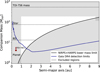 |
Fig. 9 Limits on the companion mass of TOI-756 system as a function of semi-major axis. The lower limit, indicated by the solid black line, is calculated based on the RV linear trend. The excluded gray areas include this constraint of the RV linear trend, the timespan of observations of the RV (left rectangle), the limit from high-contrast imaging (upper right rectangle), and the absence of a double peak in the CCF (upper rectangle). We plotted the Gaia DR4 astrometric detection limits as a solid dark blue line for a star at 86 pc with a RUWE of 1.25 (Wallace et al. 2025). The dotted black lines are the different mass limit categories separating planetary, brown dwarf (BD), and stellar natures. |
6.3.3 The binarity effect on formation and evolution
The presence of the widely separated stellar companion at ~11″ raises important questions about its influence on the formation and dynamical evolution of planets within the TOI-756 system.
Binarity is known to truncate the circumstellar disk, shorten its lifetime, and reduce planet occurrence rates (Cieza et al. 2009; Harris et al. 2012; Moe & Kratter 2021). While the wide physical separation between the two stars suggests that the stellar companion had a limited direct impact on the protoplanetary disk of TOI-756, studies have shown that binary companions can still influence planet formation and evolution even at separations up to 1000 au, potentially hindering the formation of massive planetary cores (Sullivan et al. 2023).
On the other hand, recent studies (Sullivan et al. 2024) show that the radius gap in wide binaries (separation > 300 au) appears to be shifted toward smaller radii. This suggests that the presence of a stellar companion can influence disk conditions and, consequently, the formation and evolution of planets.
However, despite expectations that a stellar companion at this distance could have a noticeable gravitational effect, WT 352 is significantly less massive (M⋆ ~ 0.3 M⊙) than the primary and is located at a separation that could exceed 1000 au. In this case, the companion did not inhibit the formation of giant planets or sub-stellar objects around the primary star. This suggests that the gravitational effect of a companion depends not only on its separation, but also on its mass relative to the primary star. Furthermore, while upcoming Gaia DR4 data will refine astrometric measurements, it is unlikely to provide significant new constraints on the orbital parameters of the binary, given that its expected orbital period is on the order of ~40 000 years – too long for measurable motion within Gaia’s observational timeline (El-Badry et al. 2024).
Recently, Behmard et al. (2022); Christian et al. (2022) investigated the potential alignment between the orbital planes of planetary systems and their visual binary companions. The TOI-756 system, along with its wide binary companion WT 352, is included in their sample. Christian et al. (2022) reported a significant misalignment in this system, with a mutual inclination of i = ![Mathematical equation: $\[118_{-17}^{+34}\]$](/articles/aa/full_html/2025/10/aa55684-25/aa55684-25-eq47.png) degrees (5th to 95th percentile range). While their analysis reveals an excess of aligned systems among binaries with separations less than 700 au, they find that the distribution of mutual inclinations becomes consistent with uniformity for wider binaries (a > 700 au). This could account for the observed misalignment in TOI-756, given its projected binary separation of approximately 955 au.
degrees (5th to 95th percentile range). While their analysis reveals an excess of aligned systems among binaries with separations less than 700 au, they find that the distribution of mutual inclinations becomes consistent with uniformity for wider binaries (a > 700 au). This could account for the observed misalignment in TOI-756, given its projected binary separation of approximately 955 au.
7 Conclusions
We present the “Sub-Neptunes” subprogram of the NIRPS-GTO SP2 program, which aims to improve our understanding of the diversity in composition and internal structure of small planets around M dwarfs. By enabling the study of targets hosting TESS sub-Neptune candidates with V < 15.4, NIRPS (the red arm of HARPS) expands the reach of RV follow-up beyond the traditional limits of optical spectrographs installed on 4-meter-class telescopes.
We report the first results of the RV follow-up program of the NIRPS-GTO, presenting the characterization of a two-planet system orbiting the M-dwarf TOI-756, which is the primary component of a wide binary system with the star WT 352. TOI-756 b was initially identified by TESS and subsequently confirmed with the ground-based photometry facilities LCO-CTIO and ExTrA, as well with RV measurements obtained with NIRPS and HARPS, which enabled the determination of its mass. Additionally, NIRPS and HARPS allowed the identification of a second non-transiting planet in the system TOI-756 c, as well as an supplementary RV acceleration hinting at an extra third component in the system that could be planetary as well. TOI-756 b is a sub-Neptune with a radius of 2.81 R⊕ and a mass of 9.8 M⊕ orbiting with a period of 1.24 days around its star. TOI-756 c is a cold eccentric giant planet orbiting at 149 days with a minimum mass of 4.05 MJup and an eccentricity of 0.45.
TOI-756 b, with a density of 2.42 g cm−3, is in line with the recently identified trend of low-density sub-Neptunes around M dwarfs compared to FGK dwarfs. In addition, this peculiar target lies in the radius cliff of M-dwarf planets and in the Neptune desert. TOI-756 b most likely requires a certain amount of hydrogen and helium in its atmosphere to account for its observed density, either as a pure H/He envelope or as a mixture of supercritical H2O and H/He.
The TOI-756 system is particularly unique, as it is the only known confirmed system hosting both a transiting sub-Neptune and an outer giant planet around an M dwarf. This makes it a valuable case for comparison with planet formation and evolution models, as well as for studying correlations between planetary populations and stellar parameters such as stellar mass and metallicity. In addition, TOI-756 c enhances the small population of giant planets around M dwarfs, a population whose formation mechanisms are still not fully understood. Identifying more of these planets is vital for constraining our models of their formation and evolutionary processes, providing deeper insights into the pathways that shape such systems. The astrometric measurements from the Gaia DR4 release will be key to combine with the RVs to further characterize this unique system.
TOI-756 b is also a promising candidate for future atmospheric characterization through transmission spectroscopy with JWST, which could help confirm or rule out the presence of a primordial H/He-dominated atmosphere. It also offers an opportunity to test hypotheses regarding the radius cliff and the Neptune desert population and to constrain the formation and evolution models of small planets orbiting alongside an eccentric outer companion.
In this study, we demonstrate the capabilities of the unique NIRPS and HARPS combination to obtain precise RVs of M dwarfs, enabling the confirmation and characterization of candidates detected by current photometric surveys such as TESS, as well as upcoming missions like PLATO (Rauer et al. 2014).
Acknowledgements
We thank the anonymous referee for their valuable comments, which helped improve the manuscript. This work has been carried out within the framework of the NCCR PlanetS supported by the Swiss National Science Foundation under grants 51NF40_182901 and 51NF40_205606. NJC, ÉA, AL, RD, FBa, BB, LMa, RA, LB, AB, CC, AD-B, LD, PLam, OL, LMo, JS-A, PV, TV & JPW acknowledge the financial support of the FRQ-NT through the Centre de recherche en astrophysique du Québec as well as the support from the Trottier Family Foundation and the Trottier Institute for Research on Exoplanets. ÉA, RD, FBa, LMa, TA, J-SM, MO, JS-A & PV acknowledges support from Canada Foundation for Innovation (CFI) program, the Université de Montréal and Université Laval, the Canada Economic Development (CED) program and the Ministere of Economy, Innovation and Energy (MEIE). AL acknowledges support from the Fonds de recherche du Québec (FRQ) – Secteur Nature et technologies under file #349961. The Board of Observational and Instrumental Astronomy (NAOS) at the Federal University of Rio Grande do Norte’s research activities are supported by continuous grants from the Brazilian funding agency CNPq. This study was partially funded by the Coordenação de Aperfeiçoamento de Pessoal de Nível Superior–Brasil (CAPES) – Finance Code 001 and the CAPES-Print program. 0 SCB, ED-M, NCS, EC, ARCS & JGd acknowledge the support from FCT – Fundação para a Ciência e a Tecnologia through national funds by these grants: UIDB/04434/2020, UIDP/04434/2020. Co-funded by the European Union (ERC, FIERCE, 101052347). Views and opinions expressed are however those of the author(s) only and do not necessarily reflect those of the European Union or the European Research Council. Neither the European Union nor the granting authority can be held responsible for them. SCB acknowledges the support from Fundação para a Ciência e Tecnologia (FCT) in the form of a work contract through the Scientific Employment Incentive program with reference 2023.06687.CEECIND and DOI 10.54499/2023.06687.CEECIND/CP2839/CT0002. XB, XDe, ACar, TF & VY acknowledge funding from the French ANR under contract number ANR18-CE310019 (SPlaSH), and the French National Research Agency in the framework of the Investissements d’Avenir program (ANR-15-IDEX-02), through the funding of the “Origin of Life” project of the Grenoble-Alpes University. BLCM & AMM acknowledge CAPES postdoctoral fellowships. BLCM acknowledges CNPq research fellowships (Grant No. 305804/2022-7). NBC acknowledges support from an NSERC Discovery Grant, a Canada Research Chair, and an Arthur B. McDonald Fellowship, and thanks the Trottier Space Institute for its financial support and dynamic intellectual environment. DBF acknowledges financial support from the Brazilian agency CNPq-PQ (Grant No. 305566/2021-0). Continuous grants from the Brazilian agency CNPq support the STELLAR TEAM of the Federal University of Ceara’s research activities. JRM acknowledges CNPq research fellowships (Grant No. 308928/2019-9). ED-M further acknowledges the support from FCT through Stimulus FCT contract 2021.01294.CEECIND. ED-M acknowledges the support by the Ramón y Cajal contract RyC2022-035854-I funded by MICIU/AEI/10.13039/501100011033 and by ESF+. XDu acknowledges the support from the European Research Council (ERC) under the European Union’s Horizon 2020 research and innovation programme (grant agreement SCORE No. 851555) and from the Swiss National Science Foundation under the grant SPECTRE (No 200021_215200). DE acknowledge support from the Swiss National Science Foundation for project 200021_200726. The authors acknowledge the financial support of the SNSF. JIGH, RR, ASM, FGT, NN, VMP, JLR & AKS acknowledge financial support from the Spanish Ministry of Science, Innovation and Universities (MICIU) projects PID2020-117493GB-I00 and PID2023-149982NB-I00. ICL acknowledges CNPq research fellowships (Grant No. 313103/2022-4). CMo acknowledges the funding from the Swiss National Science Foundation under grant 200021_204847 “PlanetsInTime”. KAM acknowledges support from the Swiss National Science Foundation (SNSF) under the Postdoc Mobility grant P500PT_230225. RA acknowledges the Swiss National Science Foundation (SNSF) support under the Post-Doc Mobility grant P500PT_222212 and the support of the Institut Trottier de Recherche sur les Exoplanètes (IREx). We acknowledge funding from the European Research Council under the ERC Grant Agreement n. 337591-ExTrA. LB acknowledges the support of the Natural Sciences and Engineering Research Council of Canada (NSERC). This project has received funding from the European Research Council (ERC) under the European Union’s Horizon 2020 research and innovation programme (project SPICE DUNE, grant agreement No 947634). This material reflects only the authors’ views and the Commission is not liable for any use that may be made of the information contained therein. ARCS acknowledges the support from Fundaçao para a Ciência e a Tecnologia (FCT) through the fellowship 2021.07856.BD. LD acknowledges the support of the Natural Sciences and Engineering Research Council of Canada (NSERC) and from the Fonds de recherche du Québec (FRQ) – Secteur Nature et technologies. FG acknowledges support from the Fonds de recherche du Québec (FRQ) – Secteur Nature et technologies under file #350366. HJH acknowledges funding from eSSENCE (grant number eSSENCE@LU 9:3), the Swedish National Research Council (project number 2023-05307), The Crafoord foundation and the Royal Physiographic Society of Lund, through The Fund of the Walter Gyllenberg Foundation. LMo acknowledges the support of the Natural Sciences and Engineering Research Council of Canada (NSERC), [funding reference number 589653]. NN acknowledges financial support by Light Bridges S.L, Las Palmas de Gran Canaria. NN acknowledges funding from Light Bridges for the Doctoral Thesis "Habitable Earth-like planets with ESPRESSO and NIRPS", in cooperation with the Instituto de Astrofísica de Canarias, and the use of Indefeasible Computer Rights (ICR) being commissioned at the ASTRO POC project in the Island of Tenerife, Canary Islands (Spain). The ICR-ASTRONOMY used for his research was provided by Light Bridges in cooperation with Hewlett Packard Enterprise (HPE). CPi acknowledges support from the NSERC Vanier scholarship, and the Trottier Family Foundation. CPi also acknowledges support from the E. Margaret Burbidge Prize Postdoctoral Fellowship from the Brinson Foundation. AKS acknowledges financial support from La Caixa Foundation (ID 100010434) under the grant LCF/BQ/DI23/11990071. TV acknowledges support from the Fonds de recherche du Québec (FRQ) – Secteur Nature et technologies under file #320056. KaC acknowledges support from the TESS mission via sub-award s3449 from MIT. Funding for the TESS mission is provided by NASA’s Science Mission Directorate. We acknowledge the use of public TESS data from pipelines at the TESS Science Office and at the TESS Science Processing Operations Center. Resources supporting this work were provided by the NASA High-End Computing (HEC) Program through the NASA Advanced Supercomputing (NAS) Division at Ames Research Center for the production of the SPOC data products. This research has made use of the Exoplanet Follow-up Observation Program (ExoFOP; DOI: 10.26134/ExoFOP5) website, which is operated by the California Institute of Technology, under contract with the National Aeronautics and Space Administration under the Exoplanet Exploration Program. This paper includes data collected by the TESS mission that are publicly available from the Mikulski Archive for Space Telescopes (MAST). This work makes use of observations from the LCOGT network. Part of the LCOGT telescope time was granted by NOIRLab through the Mid-Scale Innovations Program (MSIP). MSIP is funded by NSF. This research has made use of the NASA Exoplanet Archive, which is operated by the California Institute of Technology, under contract with the National Aeronautics and Space Administration under the Exoplanet Exploration Program.
Appendix A TESS pixel file plots
In this appendix, we show the TESS pixel file plots for all the sectors observed of TOI-756 (except Sector 10 shown in Fig. 1).
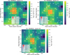 |
Fig. A.1 TESS TPF of TOI-756 created with tpfplotter (Aller et al. 2020). The orange pixels define the aperture mask used for extracting the photometry. Additionally, the red circles indicate neighboring objects from the Gaia DR3 catalog, with the circle size corresponding to the brightness difference compared to the target (as indicated in the legend). Our target is marked with a white cross. Pixel scale is 21″/pixel. The co-moving companion of TOI-756 corresponds to the star labeled "2". |
Appendix B High-contrast imaging observations
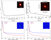 |
Fig. B.1 Adaptive optics and speckle imaging plots for TOI-756 showing magnitude contrast in function of angular separation. Top left: NACO/CONICA@VLT. Top right: HRCam@SOAR. Bottom: Zorro@Gemini-South (left: March 12, 2020; right: July 05, 2023). For VLT and Gemini, the inset image is the primary target showing no additional close-in companions. For SOAR, the inset image shows the auto-correlation function. |
Appendix C Photometric and radial velocity analysis
Median values and 68% confidence intervals of the posterior distributions of the TESS-only fit.
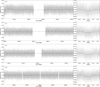 |
Fig. C.1 TESS PDCSAP flux light curves of the four different sectors with the best-fit juliet model shown as a black line (see Sect. 5.2.3 for details on the modeling). |
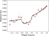 |
Fig. C.2 LCO-CTIO light curve from the g′-band transit with the best-fit juliet model shown as a black line and model errors as gray area. Dark red circles are data binned to 10 min (see Sect. 5.2.3 for details on the modeling). We do not present the i′-band transit here, as no detrending was applied, making it identical to the one shown in Fig. 5. |
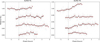 |
Fig. C.3 ExTrA light curves of the four different transits, observed with two telescopes (left panel: first telescope; right panel: second telescope). From top to bottom, the first transit is complete, while the remaining three show only the egress. The best-fit juliet models are shown as black lines, with 1σ model uncertainties indicated by the gray shaded regions. Dark red circles represent the data binned to 10 minutes. The dashed vertical line define the transit midpoint. An arbitrary offset has been added between the transits for clarity. See Sect. 5.2.3 for details on the modeling. |
Median values and 68% confidence intervals of the posterior distributions of the joint fit.
Appendix D Interior modeling of TOI-756 b
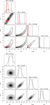 |
Fig. D.1 Corner plots from the interior modeling of TOI-756 b (see Sect.6.2.2). The top panel shows scenario (1), assuming a H/He envelope: results with uninformative priors are shown in grey, and those using stellar-informed priors based on the host star’s refractory abundances are in red. The bottom panel corresponds to scenario (2), assuming a pure H2O envelope with stellar-informed priors. |
References
- Aguichine, A., Mousis, O., Deleuil, M., & Marcq, E. 2021, ApJ, 914, 84 [NASA ADS] [CrossRef] [Google Scholar]
- Aguichine, A., Batalha, N., Fortney, J. J., et al. 2025, ApJ, 988, 186 [Google Scholar]
- Alexander, R. D., & Pascucci, I. 2012, MNRAS, 422, L82 [NASA ADS] [CrossRef] [Google Scholar]
- Alibert, Y., & Benz, W. 2017, A&A, 598, L5 [NASA ADS] [CrossRef] [EDP Sciences] [Google Scholar]
- Allard, F., Homeier, D., & Freytag, B. 2012, Philos. Trans. Roy. Soc. Lond. A, 370, 2765 [NASA ADS] [Google Scholar]
- Allart, R., Lovis, C., Faria, J., et al. 2022, A&A, 666, A196 [NASA ADS] [CrossRef] [EDP Sciences] [Google Scholar]
- Aller, A., Lillo-Box, J., Jones, D., Miranda, L. F., & Barceló Forteza, S. 2020, A&A, 635, A128 [NASA ADS] [CrossRef] [EDP Sciences] [Google Scholar]
- Ambikasaran, S., Foreman-Mackey, D., Greengard, L., Hogg, D. W., & O’Neil, M. 2015, IEEE Trans. Pattern Anal. Mach. Intell., 38, 252 [Google Scholar]
- Anglada-Escudé, G., & Butler, R. P. 2012, ApJS, 200, 15 [Google Scholar]
- Antoniadis-Karnavas, A., Sousa, S. G., Delgado-Mena, E., et al. 2020, A&A, 636, A9 [NASA ADS] [CrossRef] [EDP Sciences] [Google Scholar]
- Antoniadis-Karnavas, A., Sousa, S. G., Delgado-Mena, E., Santos, N. C., & Andreasen, D. T. 2024, A&A, 690, A58 [NASA ADS] [CrossRef] [EDP Sciences] [Google Scholar]
- Armstrong, D. J., Lopez, T. A., Adibekyan, V., et al. 2020, Nature, 583, 39 [Google Scholar]
- Artigau, E., Cadieux, C., Cook, N. J., et al. 2022, AJ, 164, 84 [NASA ADS] [CrossRef] [Google Scholar]
- Artigau, É., Cadieux, C., Cook, N. J., et al. 2024, AJ, 168, 252 [Google Scholar]
- Astudillo-Defru, N., Díaz, R. F., Bonfils, X., et al. 2017, A&A, 605, L11 [EDP Sciences] [Google Scholar]
- Baraffe, I., Chabrier, G., Allard, F., & Hauschildt, P. H. 1998, A&A, 337, 403 [Google Scholar]
- Baraffe, I., Homeier, D., Allard, F., & Chabrier, G. 2015, A&A, 577, A42 [NASA ADS] [CrossRef] [EDP Sciences] [Google Scholar]
- Batalha, N. M., Rowe, J. F., Bryson, S. T., et al. 2013, ApJS, 204, 24 [Google Scholar]
- Batalha, N. E., Lewis, T., Fortney, J. J., et al. 2019, ApJ, 885, L25 [Google Scholar]
- Bayo, A., Rodrigo, C., Barrado Y Navascués, D., et al. 2008, A&A, 492, 277 [NASA ADS] [CrossRef] [EDP Sciences] [Google Scholar]
- Behmard, A., Dai, F., & Howard, A. W. 2022, AJ, 163, 160 [NASA ADS] [CrossRef] [Google Scholar]
- Benneke, B., Roy, P.-A., Coulombe, L.-P., et al. 2024, arXiv e-prints [arXiv:2403.03325] [Google Scholar]
- Bensby, T., Feltzing, S., & Oey, M. S. 2014, A&A, 562, A71 [NASA ADS] [CrossRef] [EDP Sciences] [Google Scholar]
- Bertaux, J. L., Lallement, R., Ferron, S., Boonne, C., & Bodichon, R. 2014, A&A, 564, A46 [NASA ADS] [CrossRef] [EDP Sciences] [Google Scholar]
- Bitsch, B., & Izidoro, A. 2023, A&A, 674, A178 [NASA ADS] [CrossRef] [EDP Sciences] [Google Scholar]
- Bitsch, B., Lambrechts, M., & Johansen, A. 2015, A&A, 582, A112 [NASA ADS] [CrossRef] [EDP Sciences] [Google Scholar]
- Bitsch, B., Raymond, S. N., Buchhave, L. A., et al. 2021, A&A, 649, L5 [NASA ADS] [CrossRef] [EDP Sciences] [Google Scholar]
- Bonfils, X., Delfosse, X., Udry, S., et al. 2013, A&A, 549, A109 [NASA ADS] [CrossRef] [EDP Sciences] [Google Scholar]
- Bonfils, X., Almenara, J. M., Jocou, L., et al. 2015, SPIE Conf. Ser., 9605, 96051L [NASA ADS] [Google Scholar]
- Borucki, W. J., Koch, D., Basri, G., et al. 2010, Science, 327, 977 [Google Scholar]
- Borucki, W. J., Koch, D. G., Basri, G., et al. 2011, ApJ, 736, 19 [Google Scholar]
- Bouchy, F., Doyon, R., Artigau, É., et al. 2017, The Messenger, 169, 21 [NASA ADS] [Google Scholar]
- Bouchy, F., Doyon, R., Pepe, F., Melo, C., & Artigau, É. 2025, A&A, 700, A10 [NASA ADS] [CrossRef] [EDP Sciences] [Google Scholar]
- Brahm, R., Espinoza, N., Jordán, A., et al. 2018, MNRAS, 477, 2572 [Google Scholar]
- Brown, T. M., Baliber, N., Bianco, F. B., et al. 2013, PASP, 125, 1031 [Google Scholar]
- Brugger, B., Mousis, O., Deleuil, M., & Deschamps, F. 2017, ApJ, 850, 93 [NASA ADS] [CrossRef] [Google Scholar]
- Bryan, M. L., & Lee, E. J. 2024, ApJ, 968, L25 [NASA ADS] [CrossRef] [Google Scholar]
- Bryan, M. L., & Lee, E. J. 2025, ApJ, 982, L7 [Google Scholar]
- Bryant, E. M., Bayliss, D., & Van Eylen, V. 2023, MNRAS, 521, 3663 [CrossRef] [Google Scholar]
- Burn, R., Schlecker, M., Mordasini, C., et al. 2021, A&A, 656, A72 [NASA ADS] [CrossRef] [EDP Sciences] [Google Scholar]
- Burn, R., Mordasini, C., Mishra, L., et al. 2024, Nat. Astron., 8, 463 [Google Scholar]
- Castelli, F., & Kurucz, R. L. 2003, in Modelling of Stellar Atmospheres, eds. N. Piskunov, W. W. Weiss, & D. F. Gray, IAU Symposium, 210, A20 [NASA ADS] [Google Scholar]
- Castro-González, A., Bourrier, V., Lillo-Box, J., et al. 2024, A&A, 689, A250 [NASA ADS] [CrossRef] [EDP Sciences] [Google Scholar]
- Chachan, Y., & Lee, E. J. 2023, ApJ, 952, L20 [NASA ADS] [CrossRef] [Google Scholar]
- Christian, S., Vanderburg, A., Becker, J., et al. 2022, AJ, 163, 207 [NASA ADS] [CrossRef] [Google Scholar]
- Ciardi, D. R., Beichman, C. A., Horch, E. P., & Howell, S. B. 2015, ApJ, 805, 16 [NASA ADS] [CrossRef] [Google Scholar]
- Cieza, L. A., Padgett, D. L., Allen, L. E., et al. 2009, ApJ, 696, L84 [NASA ADS] [CrossRef] [Google Scholar]
- Cloutier, R., & Menou, K. 2020, AJ, 159, 211 [NASA ADS] [CrossRef] [Google Scholar]
- Cointepas, M., Almenara, J. M., Bonfils, X., et al. 2021, A&A, 650, A145 [NASA ADS] [CrossRef] [EDP Sciences] [Google Scholar]
- Collins, K. 2019, in American Astronomical Society Meeting Abstracts, 233, 140.05 [NASA ADS] [Google Scholar]
- Collins, K. A., Kielkopf, J. F., Stassun, K. G., & Hessman, F. V. 2017, AJ, 153, 77 [Google Scholar]
- Cook, N. J., Artigau, É., Doyon, R., et al. 2022, PASP, 134, 114509 [NASA ADS] [CrossRef] [Google Scholar]
- Deline, A., Hooton, M. J., Lendl, M., et al. 2022, A&A, 659, A74 [NASA ADS] [CrossRef] [EDP Sciences] [Google Scholar]
- Delmotte, N., Dolensky, M., Padovani, P., et al. 2006, in Astronomical Society of the Pacific Conference Series, 351, 690 [NASA ADS] [Google Scholar]
- Donati, J. F., Kouach, D., Moutou, C., et al. 2020, MNRAS, 498, 5684 [Google Scholar]
- Dorn, C., Khan, A., Heng, K., et al. 2015, A&A, 577, A83 [NASA ADS] [CrossRef] [EDP Sciences] [Google Scholar]
- Dressing, C. D., & Charbonneau, D. 2013, ApJ, 767, 95 [Google Scholar]
- Dressing, C. D., & Charbonneau, D. 2015, ApJ, 807, 45 [Google Scholar]
- El-Badry, K., Rix, H.-W., & Heintz, T. M. 2021, MNRAS, 506, 2269 [NASA ADS] [CrossRef] [Google Scholar]
- El-Badry, K., Lam, C., Holl, B., et al. 2024, Open J. Astrophys., 7, 100 [Google Scholar]
- Espinoza, N. 2018, RNAAS, 2, 209 [Google Scholar]
- Espinoza, N., & Jordán, A. 2015, MNRAS, 450, 1879 [Google Scholar]
- Espinoza, N., Kossakowski, D., & Brahm, R. 2019, MNRAS, 490, 2262 [Google Scholar]
- Foreman-Mackey, D., Hogg, D. W., Lang, D., & Goodman, J. 2013, PASP, 125, 306 [Google Scholar]
- Foreman-Mackey, D., Agol, E., Ambikasaran, S., & Angus, R. 2017, AJ, 154, 220 [Google Scholar]
- French, M., Mattsson, T. R., Nettelmann, N., & Redmer, R. 2009, Phys. Rev. B, 79, 054107 [NASA ADS] [CrossRef] [Google Scholar]
- Fulton, B. J., Petigura, E. A., Howard, A. W., et al. 2017, AJ, 154, 109 [Google Scholar]
- Fulton, B. J., Petigura, E. A., Blunt, S., & Sinukoff, E. 2018, PASP, 130, 044504 [Google Scholar]
- Gaia Collaboration (Brown, A. G. A., et al.) 2018, A&A, 616, A1 [NASA ADS] [CrossRef] [EDP Sciences] [Google Scholar]
- Gaidos, E., Mann, A. W., Kraus, A. L., & Ireland, M. 2016, MNRAS, 457, 2877 [Google Scholar]
- Gardner, J. P., Mather, J. C., Clampin, M., et al. 2006, Space Sci. Rev., 123, 485 [Google Scholar]
- Gordon, I. E., Rothman, L. S., Hargreaves, R. J., et al. 2022, J. Quant. Spec. Radiat. Transf., 277, 107949 [NASA ADS] [CrossRef] [Google Scholar]
- Gratia, P., & Fabrycky, D. 2017, MNRAS, 464, 1709 [NASA ADS] [CrossRef] [Google Scholar]
- Guerrero, N. M., Seager, S., Huang, C. X., et al. 2021, ApJS, 254, 39 [NASA ADS] [CrossRef] [Google Scholar]
- Guillot, T., & Morel, P. 1995, A&AS, 109, 109 [NASA ADS] [Google Scholar]
- Hara, N. C., Boué, G., Laskar, J., Delisle, J. B., & Unger, N. 2019, MNRAS, 489, 738 [Google Scholar]
- Harris, R. J., Andrews, S. M., Wilner, D. J., & Kraus, A. L. 2012, ApJ, 751, 115 [Google Scholar]
- Hedges, C., Saunders, N., Barentsen, G., et al. 2019, ApJ, 880, L5 [NASA ADS] [CrossRef] [Google Scholar]
- Henden, A. A., Levine, S., Terrell, D., & Welch, D. L. 2015, in American Astronomical Society Meeting Abstracts, 225, 336.16 [NASA ADS] [Google Scholar]
- Henry, T. J., Jao, W.-C., Subasavage, J. P., et al. 2006, AJ, 132, 2360 [Google Scholar]
- Ho, C. S. K., Rogers, J. G., Van Eylen, V., Owen, J. E., & Schlichting, H. E. 2024, MNRAS, 531, 3698 [NASA ADS] [CrossRef] [Google Scholar]
- Howard, A. W., Marcy, G. W., Bryson, S. T., et al. 2012, ApJS, 201, 15 [Google Scholar]
- Howell, S. B., Everett, M. E., Sherry, W., Horch, E., & Ciardi, D. R. 2011, AJ, 142, 19 [Google Scholar]
- Husser, T.-O., Wende-von Berg, S., Dreizler, S., et al. 2013, A&A, 553, A6 [NASA ADS] [CrossRef] [EDP Sciences] [Google Scholar]
- Ida, S., & Lin, D. N. C. 2005, ApJ, 626, 1045 [NASA ADS] [CrossRef] [Google Scholar]
- Jahandar, F., Doyon, R., Artigau, É., et al. 2024, ApJ, 966, 56 [CrossRef] [Google Scholar]
- Jahandar, F., Doyon, R., Artigau, É., et al. 2025, ApJ, 978, 154 [Google Scholar]
- Jenkins, J. M., Twicken, J. D., McCauliff, S., et al. 2016, SPIE Conf. Ser.,. 9913, 99133E [Google Scholar]
- Kempton, E. M. R., Bean, J. L., Louie, D. R., et al. 2018, PASP, 130, 114401 [Google Scholar]
- Khata, D., Mondal, S., Das, R., & Baug, T. 2021, MNRAS, 507, 1869 [NASA ADS] [CrossRef] [Google Scholar]
- Kite, E. S., Fegley, Jr., B., Schaefer, L., & Ford, E. B. 2019, ApJ, 887, L33 [NASA ADS] [CrossRef] [Google Scholar]
- Kreidberg, L. 2015, PASP, 127, 1161 [Google Scholar]
- Kubyshkina, D., & Vidotto, A. A. 2021, MNRAS, 504, 2034 [NASA ADS] [CrossRef] [Google Scholar]
- Kunimoto, M., Vanderburg, A., Huang, C. X., et al. 2023, AJ, 166, 7 [NASA ADS] [CrossRef] [Google Scholar]
- Kurucz, R. L. 1979, ApJS, 40, 1 [NASA ADS] [CrossRef] [Google Scholar]
- Kurucz, R. L. 1993, SYNTHE spectrum synthesis programs and line data [Google Scholar]
- Laughlin, G., Bodenheimer, P., & Adams, F. C. 2004, ApJ, 612, L73 [NASA ADS] [CrossRef] [Google Scholar]
- Lenzen, R., Hartung, M., Brandner, W., et al. 2003, SPIE Conf. Ser., 4841, 944 [Google Scholar]
- Li, J., Tenenbaum, P., Twicken, J. D., et al. 2019, PASP, 131, 024506 [NASA ADS] [CrossRef] [Google Scholar]
- Lillo-Box, J., Gandolfi, D., Armstrong, D. J., et al. 2023, A&A, 669, A109 [NASA ADS] [CrossRef] [EDP Sciences] [Google Scholar]
- Lopez, E. D., & Fortney, J. J. 2013, ApJ, 776, 2 [Google Scholar]
- Lopez, E. D., & Rice, K. 2018, MNRAS, 479, 5303 [NASA ADS] [CrossRef] [Google Scholar]
- Lovis, C., & Pepe, F. 2007, A&A, 468, 1115 [NASA ADS] [CrossRef] [EDP Sciences] [Google Scholar]
- Lucy, L. B., & Sweeney, M. A. 1971, AJ, 76, 544 [NASA ADS] [CrossRef] [Google Scholar]
- Luo, H., Dorn, C., & Deng, J. 2024, Nat. Astron., 8, 1399 [Google Scholar]
- Mann, H. B., & Whitney, D. R. 1947, Ann. Math. Statist., 18, 50 [CrossRef] [Google Scholar]
- Mann, A. W., Feiden, G. A., Gaidos, E., Boyajian, T., & von Braun, K. 2015, ApJ, 804, 64 [Google Scholar]
- Mann, A. W., Dupuy, T., Kraus, A. L., et al. 2019, ApJ, 871, 63 [Google Scholar]
- Marcy, G. W., Weiss, L. M., Petigura, E. A., et al. 2014, PNAS, 111, 12655 [NASA ADS] [CrossRef] [Google Scholar]
- Mayor, M., & Queloz, D. 1995, Nature, 378, 355 [Google Scholar]
- Mayor, M., Pepe, F., Queloz, D., et al. 2003, The Messenger, 114, 20 [NASA ADS] [Google Scholar]
- McCully, C., Volgenau, N. H., Harbeck, D.-R., et al. 2018, SPIE Conf. Ser., 10707, 107070K [Google Scholar]
- McDonald, G. D., Kreidberg, L., & Lopez, E. 2019, ApJ, 876, 22 [Google Scholar]
- McLaughlin, D. B. 1924, ApJ, 60, 22 [Google Scholar]
- Mignon, L., Delfosse, X., Meunier, N., et al. 2025, A&A, in press [Google Scholar]
- Moe, M., & Kratter, K. M. 2021, MNRAS, 507, 3593 [NASA ADS] [CrossRef] [Google Scholar]
- Morello, G., Tsiaras, A., Howarth, I. D., & Homeier, D. 2017, AJ, 154, 111 [NASA ADS] [CrossRef] [Google Scholar]
- Morris, R. L., Twicken, J. D., Smith, J. C., et al. 2020, Kepler Data Processing Handbook: Photometric Analysis, Kepler Science Document KSCI-19081-003, 6, ed. J. M. Jenkins [Google Scholar]
- Mugrauer, M., & Michel, K.-U. 2020, Astron. Nachr., 341, 996 [NASA ADS] [CrossRef] [Google Scholar]
- Mulders, G. D., Pascucci, I., & Apai, D. 2015, ApJ, 814, 130 [NASA ADS] [CrossRef] [Google Scholar]
- Neves, V., Bonfils, X., Santos, N. C., et al. 2012, A&A, 538, A25 [NASA ADS] [CrossRef] [EDP Sciences] [Google Scholar]
- Neves, V., Bonfils, X., Santos, N. C., et al. 2013, A&A, 551, A36 [NASA ADS] [CrossRef] [EDP Sciences] [Google Scholar]
- Otegi, J. F., Bouchy, F., & Helled, R. 2020, A&A, 634, A43 [NASA ADS] [CrossRef] [EDP Sciences] [Google Scholar]
- Owen, J. E., & Jackson, A. P. 2012, MNRAS, 425, 2931 [Google Scholar]
- Owen, J. E., & Murray-Clay, R. 2018, MNRAS, 480, 2206 [NASA ADS] [CrossRef] [Google Scholar]
- Owen, J. E., & Wu, Y. 2017, ApJ, 847, 29 [Google Scholar]
- Parc, L., Bouchy, F., Venturini, J., Dorn, C., & Helled, R. 2024, A&A, 688, A59 [NASA ADS] [CrossRef] [EDP Sciences] [Google Scholar]
- Pascucci, I., Testi, L., Herczeg, G. J., et al. 2016, ApJ, 831, 125 [Google Scholar]
- Pass, E. K., Winters, J. G., Charbonneau, D., et al. 2023, AJ, 166, 11 [NASA ADS] [CrossRef] [Google Scholar]
- Pecaut, M. J., & Mamajek, E. E. 2013, ApJS, 208, 9 [Google Scholar]
- Pepe, F., Cristiani, S., Rebolo, R., et al. 2021, A&A, 645, A96 [NASA ADS] [CrossRef] [EDP Sciences] [Google Scholar]
- Petigura, E. A., Howard, A. W., & Marcy, G. W. 2013, PNAS, 110, 19273 [NASA ADS] [CrossRef] [Google Scholar]
- Plotnykov, M., & Valencia, D. 2020, MNRAS, 499, 932 [CrossRef] [Google Scholar]
- Plotnykov, M., & Valencia, D. 2024, MNRAS, 530, 3488 [Google Scholar]
- Pojmanski, G. 1997, Acta Astron., 47, 467 [Google Scholar]
- Rasio, F. A., & Ford, E. B. 1996, Science, 274, 954 [Google Scholar]
- Rauer, H., Catala, C., Aerts, C., et al. 2014, Exp. Astron., 38, 249 [Google Scholar]
- Raymond, S. N., & Izidoro, A. 2017, Icarus, 297, 134 [CrossRef] [Google Scholar]
- Reylé, C., Jardine, K., Fouqué, P., et al. 2021, A&A, 650, A201 [Google Scholar]
- Ribas, I., Guinan, E. F., Güdel, M., & Audard, M. 2005, ApJ, 622, 680 [Google Scholar]
- Ricker, G. R., Winn, J. N., Vanderspek, R., et al. 2014, SPIE Conf. Ser., 9143, 914320 [Google Scholar]
- Rossiter, R. A. 1924, ApJ, 60, 15 [Google Scholar]
- Rousset, G., Lacombe, F., Puget, P., et al. 2003, SPIE Conf. Ser., 4839, 140 [Google Scholar]
- Saumon, D., Chabrier, G., & van Horn, H. M. 1995, ApJS, 99, 713 [NASA ADS] [CrossRef] [Google Scholar]
- Schlecker, M., Mordasini, C., Emsenhuber, A., et al. 2021, A&A, 656, A71 [NASA ADS] [CrossRef] [EDP Sciences] [Google Scholar]
- Schönrich, R., Binney, J., & Dehnen, W. 2010, MNRAS, 403, 1829 [NASA ADS] [CrossRef] [Google Scholar]
- Schweitzer, A., Passegger, V. M., Cifuentes, C., et al. 2019, A&A, 625, A68 [NASA ADS] [CrossRef] [EDP Sciences] [Google Scholar]
- Skrutskie, M. F., Cutri, R. M., Stiening, R., et al. 2006, AJ, 131, 1163 [NASA ADS] [CrossRef] [Google Scholar]
- Smith, J. C., Stumpe, M. C., Van Cleve, J. E., et al. 2012, PASP, 124, 1000 [Google Scholar]
- Sousa, S. G., Adibekyan, V., Delgado-Mena, E., et al. 2021, A&A, 656, A53 [NASA ADS] [CrossRef] [EDP Sciences] [Google Scholar]
- Speagle, J. S. 2020, MNRAS, 493, 3132 [Google Scholar]
- Stassun, K. G., Oelkers, R. J., Paegert, M., et al. 2019, AJ, 158, 138 [Google Scholar]
- Stumpe, M. C., Smith, J. C., Van Cleve, J. E., et al. 2012, PASP, 124, 985 [Google Scholar]
- Stumpe, M. C., Smith, J. C., Catanzarite, J. H., et al. 2014, PASP, 126, 100 [Google Scholar]
- Suárez Mascareño, A., Rebolo, R., González Hernández, J. I., & Esposito, M. 2015, MNRAS, 452, 2745 [Google Scholar]
- Suárez Mascareño, A., Rebolo, R., & González Hernández, J. I. 2016, A&A, 595, A12 [Google Scholar]
- Suárez Mascareño, A., Artigau, É., Mignon, L., Delfosse, X., & Cook, N. J. 2025, A&A, 700, A11 [NASA ADS] [CrossRef] [EDP Sciences] [Google Scholar]
- Sullivan, K., Kraus, A. L., Huber, D., et al. 2023, AJ, 165, 177 [NASA ADS] [Google Scholar]
- Sullivan, K., Kraus, A. L., Berger, T. A., et al. 2024, AJ, 168, 129 [Google Scholar]
- Tian, F., Toon, O. B., Pavlov, A. A., & De Sterck, H. 2005, ApJ, 621, 1049 [Google Scholar]
- Tokovinin, A. 2018, PASP, 130, 035002 [Google Scholar]
- Torres, G. 1999, PASP, 111, 169 [NASA ADS] [CrossRef] [Google Scholar]
- Twicken, J. D., Clarke, B. D., Bryson, S. T., et al. 2010, SPIE Conf. Ser., 7740, 774023 [NASA ADS] [Google Scholar]
- Twicken, J. D., Catanzarite, J. H., Clarke, B. D., et al. 2018, PASP, 130, 064502 [Google Scholar]
- Valencia, D., Sasselov, D. D., & O’Connell, R. J. 2007, ApJ, 656, 545 [Google Scholar]
- Venturini, J., Guilera, O. M., Haldemann, J., Ronco, M. P., & Mordasini, C. 2020, A&A, 643, L1 [NASA ADS] [CrossRef] [EDP Sciences] [Google Scholar]
- Venturini, J., Ronco, M. P., Guilera, O. M., et al. 2024, A&A, 686, L9 [NASA ADS] [CrossRef] [EDP Sciences] [Google Scholar]
- Wallace, A. L., Casey, A. R., Brown, A. G. A., & Castro-Ginard, A. 2025, MNRAS, 536, 2485 [Google Scholar]
- Weiss, L. M., Isaacson, H., Howard, A. W., et al. 2024, ApJS, 270, 8 [NASA ADS] [CrossRef] [Google Scholar]
- Wilcoxon, F. 1945, Biometrics Bull., 1, 80 [Google Scholar]
- Wilson, T. G., Goffo, E., Alibert, Y., et al. 2022, MNRAS, 511, 1043 [NASA ADS] [CrossRef] [Google Scholar]
- Winters, J. G., Henry, T. J., Lurie, J. C., et al. 2015, AJ, 149, 5 [Google Scholar]
- Wright, E. L., Eisenhardt, P. R. M., Mainzer, A. K., et al. 2010, AJ, 140, 1868 [Google Scholar]
- Wroblewski, H., & Torres, C. 1991, A&AS, 91, 129 [Google Scholar]
- Wu, Y., & Murray, N. 2003, ApJ, 589, 605 [Google Scholar]
- Wu, Y., & Lithwick, Y. 2011, ApJ, 735, 109 [Google Scholar]
- Yelle, R. V. 2004, Icarus, 170, 167 [NASA ADS] [CrossRef] [Google Scholar]
- Zeng, L., Sasselov, D. D., & Jacobsen, S. B. 2016, ApJ, 819, 127 [Google Scholar]
- Zeng, L., Jacobsen, S. B., Sasselov, D. D., et al. 2019, PNAS, 116, 9723 [Google Scholar]
- Ziegler, C., Tokovinin, A., Briceño, C., et al. 2020, AJ, 159, 19 [Google Scholar]
IRAF is distributed by National Optical Astronomy Observatories, operated by the Association of Universities for Research in Astronomy, Inc., under contract with the National Science Foundation, USA.
ULSR is directed radially inwards towards the Galactic center, VLSR along the direction of Galactic rotation, and WLSR vertically upwards towards the Galactic North pole.
All Tables
Median values and 68% confidence intervals of the posterior distributions of the TESS-only fit.
Median values and 68% confidence intervals of the posterior distributions of the joint fit.
All Figures
|
Fig. 1 TESS TPF of TOI-756 created with tpfplotter (Aller et al. 2020). The orange pixels define the aperture mask used for extracting the photometry. Additionally, the red circles indicate neighboring objects from the Gaia DR3 catalog, with the circle size corresponding to the brightness difference compared to the target (as indicated in the legend). Our target is marked with a white cross. Pixel scale is 21″/pixel. The co-moving companion of TOI-756 corresponds to the star labeled “2”. |
| In the text | |
|
Fig. 2 SED of TOI-756, constructed using broadband photometric data from APASS (magenta), Gaia (green), 2MASS (black), and WISE (blue). The upper limit for the WISE W4 band is indicated by a red dot. The horizontal error bars represent the passband widths of the respective filters. Below the SED, the residuals are shown, normalized to the photometric errors. The SED was modeled using the BT Settl atmospheric model (Allard et al. 2012) with Teff = 3600 K, [M/H] = 0 dex, and log g⋆ = 4.5 cm s−2. |
| In the text | |
|
Fig. 3 RV data from HARPS (blue dots) and NIRPS measurements. The NIRPS data is separated in unaffected datapoints (orange dots) and affected datapoints (red triangles) by the crossing of the Vsyst and BERV velocities during the observations. Yellow dots are NIRPS data with the correction explained in Sect. 5.2.2. The dotted red line together with the right y axis represent the total velocity of TOI-756, showing the crossing of the BERV with the Vsyst. The complete inferred model in Sect. 5.2.3, which comprises signals from the two planets along with the linear model for the acceleration (in gray), is represented by a black solid line. |
| In the text | |
|
Fig. 4 NIRPS data residuals (upper panel) and LBL indicators D2V (middle panel), along with dTemp (ΔT) calculated at 3500 K close to the effective temperature of TOI-756 (bottom panel). Orange dots are the indicators from unaffected NIRPS data, red triangles are the affected spectra by Vsyst−BERV crossing and yellow dots are the indicators with the correction explained in Sect. 5.2.2. |
| In the text | |
|
Fig. 5 Top panel: phase-folded TESS, ExTrA, and LCO-CTIO light curves of TOI-756 b (gray points). Dark red circles are data binned to 10 min. The black lines represent the median model of each instrument from the joint fit. Bottom panel: residuals of the data compared to the model. An arbitrary offset has been added to the ground-based photometry for clarity. |
| In the text | |
|
Fig. 6 Phase-folded RVs with the resulting model and its residuals for TOI-756 b (left) and TOI-756 c (right). In red dots, binned data combining HARPS (blue dots) and NIRPS (yellow dots). The error-bars in light gray account for the fitted jitters. |
| In the text | |
|
Fig. 7 Mass-radius diagram of small exoplanets (with radii ranging from 1–4 R⊕) with precise densities from the PlanetS catalog. The red (gray) dots correspond to exoplanets orbiting M dwarfs (FGK dwarfs). The composition lines of pure silicates (yellow dashed), Earth-like planets (red dashed), and pure iron (solid black) from Zeng et al. (2016, 2019) are displayed. The red hexagon represent TOI-756 b. Two compositions line that incorporate both water and terrestrial elements from Aguichine et al. (2021) models, matching the equilibrium temperature of the planet, are plotted as light and dark blue dotted lines. Two compositions of Earth with an hydrogen-rich atmospheres from Zeng et al. (2019) are represented in pink and purple dotted lines. This plot has been generated with mr-plotter (https://github.com/castro-gzlz/mr-plotter/). |
| In the text | |
|
Fig. 8 Planet radius as a function of orbital period for known exoplanets from NASA Exoplanet Archive with a radius precision below 8%. We highlighted the Neptunian desert, ridge, and savanna regions from Castro-González et al. (2024). The colorcode represents the observed density of planets. TOI-756 b is depicted as a dark red hexagon. Light blue symbols represent sub-Neptunes in systems hosting eccentric giant companions: crosses indicate systems with only giant planets, while circles correspond to systems containing both small and giant planets. In contrast, dark blue circles represent sub-Neptunes in systems with non-eccentric giant planets. The description of the selection is made in Sect. 6.3.1. This plot has been generated with nep-des (https://github.com/castro-gzlz/nep-des/). |
| In the text | |
|
Fig. 9 Limits on the companion mass of TOI-756 system as a function of semi-major axis. The lower limit, indicated by the solid black line, is calculated based on the RV linear trend. The excluded gray areas include this constraint of the RV linear trend, the timespan of observations of the RV (left rectangle), the limit from high-contrast imaging (upper right rectangle), and the absence of a double peak in the CCF (upper rectangle). We plotted the Gaia DR4 astrometric detection limits as a solid dark blue line for a star at 86 pc with a RUWE of 1.25 (Wallace et al. 2025). The dotted black lines are the different mass limit categories separating planetary, brown dwarf (BD), and stellar natures. |
| In the text | |
|
Fig. A.1 TESS TPF of TOI-756 created with tpfplotter (Aller et al. 2020). The orange pixels define the aperture mask used for extracting the photometry. Additionally, the red circles indicate neighboring objects from the Gaia DR3 catalog, with the circle size corresponding to the brightness difference compared to the target (as indicated in the legend). Our target is marked with a white cross. Pixel scale is 21″/pixel. The co-moving companion of TOI-756 corresponds to the star labeled "2". |
| In the text | |
|
Fig. B.1 Adaptive optics and speckle imaging plots for TOI-756 showing magnitude contrast in function of angular separation. Top left: NACO/CONICA@VLT. Top right: HRCam@SOAR. Bottom: Zorro@Gemini-South (left: March 12, 2020; right: July 05, 2023). For VLT and Gemini, the inset image is the primary target showing no additional close-in companions. For SOAR, the inset image shows the auto-correlation function. |
| In the text | |
|
Fig. C.1 TESS PDCSAP flux light curves of the four different sectors with the best-fit juliet model shown as a black line (see Sect. 5.2.3 for details on the modeling). |
| In the text | |
|
Fig. C.2 LCO-CTIO light curve from the g′-band transit with the best-fit juliet model shown as a black line and model errors as gray area. Dark red circles are data binned to 10 min (see Sect. 5.2.3 for details on the modeling). We do not present the i′-band transit here, as no detrending was applied, making it identical to the one shown in Fig. 5. |
| In the text | |
|
Fig. C.3 ExTrA light curves of the four different transits, observed with two telescopes (left panel: first telescope; right panel: second telescope). From top to bottom, the first transit is complete, while the remaining three show only the egress. The best-fit juliet models are shown as black lines, with 1σ model uncertainties indicated by the gray shaded regions. Dark red circles represent the data binned to 10 minutes. The dashed vertical line define the transit midpoint. An arbitrary offset has been added between the transits for clarity. See Sect. 5.2.3 for details on the modeling. |
| In the text | |
|
Fig. D.1 Corner plots from the interior modeling of TOI-756 b (see Sect.6.2.2). The top panel shows scenario (1), assuming a H/He envelope: results with uninformative priors are shown in grey, and those using stellar-informed priors based on the host star’s refractory abundances are in red. The bottom panel corresponds to scenario (2), assuming a pure H2O envelope with stellar-informed priors. |
| In the text | |
Current usage metrics show cumulative count of Article Views (full-text article views including HTML views, PDF and ePub downloads, according to the available data) and Abstracts Views on Vision4Press platform.
Data correspond to usage on the plateform after 2015. The current usage metrics is available 48-96 hours after online publication and is updated daily on week days.
Initial download of the metrics may take a while.