| Issue |
A&A
Volume 702, October 2025
|
|
|---|---|---|
| Article Number | A273 | |
| Number of page(s) | 15 | |
| Section | Interstellar and circumstellar matter | |
| DOI | https://doi.org/10.1051/0004-6361/202555833 | |
| Published online | 27 October 2025 | |
LMC+: Large-scale mapping of [C II] and [O III] in the LMC molecular ridge
I. Dataset and line ratio analyses
1
Deutsches SOFIA Institut, University of Stuttgart,
Pfaffenwaldring 29,
70569
Stuttgart,
Germany
2
IRAM – Institut de Radioastronomie Millimétrique,
300 rue de la Piscine,
38406
Saint-Martin d’Hères,
France
3
Université Paris Cité, Université Paris-Saclay, CEA, CNRS, AIM,
91191
Gif-sur-Yvette,
France
4
Institute of Space Systems – SOFIA Data Center, University of Stuttgart,
Pfaffenwaldring 29,
70569
Stuttgart,
Germany
5
SOFIA Science Center, USRA, NASA Ames Research Center,
M.S. N232-12
Moffett Field,
CA
94035,
USA
6
Space Telescope Science Institute,
3700 San Martin Dr.,
Baltimore,
MD
21218,
USA
7
Max-Planck-Institut für Radioastronomie,
Auf dem Hügel 69,
53121
Bonn,
Germany
8
University of Cincinnati, Clermont College,
4200 Clermont College Drive,
Batavia,
OH
45103,
USA
9
Argelander-Institut für Astronomie,
Auf dem Hügel 71,
53121
Bonn,
Germany
10
Department of Astronomy, University of Maryland,
College Park,
MD
20742,
USA
11
Universität Heidelberg, Zentrum f. Astronomie, Institut f. Theoretische Astrophysik,
A.-Ueberle-Str 2,
69120
Heidelberg,
Germany
12
Cosmic Origins Of Life (COOL) Research DAO, coolresearch.io
13
Astronomy Department, University of Illinois,
Urbana,
IL
61801,
USA
14
CNRS, IRAP,
9 Av. du Colonel Roche, BP 44346,
31028
Toulouse cedex 4,
France
15
Department of Astronomy, University of Virginia,
PO Box 3818,
Charlottesville,
VA
22903,
USA
16
Lockheed Martin Solar & Astrophysics Laboratory,
Palo Alto,
CA
94304,
USA
17
Université Paris-Saclay, Université Paris-Cité, CEA, CNRS, AIM,
91191
Gif-sur-Yvette,
France
18
Astro Space Center of P.N. Lebedev Physics Institute (ACS LPI),
Moscow
117997,
Russia
19
Space Science Institute,
4765 Walnut Street, Suite 205,
Boulder,
CO
80301,
USA
20
Departamento de Astronomía, Universidad de Chile,
Casilla 36-D,
Santiago,
Chile
21
NSF’s NOIRLab,
950 N. Cherry Avenue,
Tucson,
AZ
85719,
USA
22
Universidad Autónoma de Chile, Nucleo Astroquimica y Astrofisica,
Avda Pedro de Valdivia 425,
Providencia, Santiago de Chile,
Chile
★ Corresponding author: This email address is being protected from spambots. You need JavaScript enabled to view it.
Received:
5
June
2025
Accepted:
1
September
2025
Abstract
Context. The fundamental process of star formation in galaxies involves the intricate interplay between the fueling of star formation via molecular gas and the feedback from recently formed massive stars that can, in turn, hinder the conversion of gas into stars. This process, by which galaxies evolve, is also closely connected to the intrinsic properties of the interstellar medium (ISM), such as structure, density, pressure, and metallicity.
Aims. To study the role that different molecular and atomic phases of the ISM play in star formation, and to characterize their physical conditions, we zoom into our nearest neighboring galaxy, the Large Magellanic Cloud (LMC; 50 kpc), the most convenient laboratory in which to study the effects of the lower metal abundance on the properties of the ISM. The LMC offers a view of the ISM and star formation conditions in a low-metallicity (Z ~ 0.5 Z⊙) environment similar, in that regard, to the epoch of the peak of star formation in the earlier Universe (z ~ 1.5). Following up on studies carried out at galactic scales in low-Z galaxies, we present an unprecedentedly detailed analysis of well-known star-forming regions (SFRs) at a spatial resolution of a few parsecs.
Methods. We mapped a 610pc × 260pc region in the LMC molecular ridge in [C II]λ158 µm and the [O III]λ88 µm using the FIFI-LS instrument on the SOFIA telescope. We compared the data with the distribution of the CO(2−1) emission from ALMA, the modeled total infrared luminosity, and the Spitzer/MIPS 24 µm continuum and Hα.
Results. We present new large maps of [C II] and [O III] and perform a first comparison with CO(2−1) line and LTIR emission. We also provide a detailed description of the observing strategy with SOFIA/FIFI-LS and the data reduction process.
Conclusions. We find that [C II] and [O III] emission is associated with the SFRs in the molecular ridge, but also extends throughout the mapped region, and is not obviously associated with ongoing star formation. The CO emission is clumpier than the [C II] emission and we find plentiful [C II] present where there is little CO emission, possibly holding important implications for “CO-dark” gas. We find a clear trend of the L[C II]/LTIR ratio decreasing with increasing LTIR in the full range. This suggests a strong link between the “[C II]-deficit” and the local physical conditions instead of global properties.
Key words: methods: data analysis / ISM: general / galaxies: ISM
© The Authors 2025
 Open Access article, published by EDP Sciences, under the terms of the Creative Commons Attribution License (https://creativecommons.org/licenses/by/4.0), which permits unrestricted use, distribution, and reproduction in any medium, provided the original work is properly cited.
This article is published in open access under the Subscribe to Open model. This email address is being protected from spambots. You need JavaScript enabled to view it. to support open access publication.
1 Introduction
The necessary fuel to feed star formation is considered to be molecular gas, as is evidenced, for example, by the Kennicutt-Schmidt relationship (Kennicutt 1998). As molecular hydrogen cannot be observed directly, the carbon monoxide (CO) J=1−0 transition has traditionally been the convenient tracer of total molecular gas and is thus a calibrator of star formation activity in the local Universe as well as at high redshifts. However, this leads to puzzling results in low-metallicity (low-Z) galaxies. There the relation of molecular gas traced by CO (1−0) to the efficiency with which these galaxies form stars is perplexing. This is mainly due to the fact that the search for CO (1−0) in low-Z galaxies is a veritable challenge (e.g., Cormier et al. 2014; Madden et al. 2020), making the conversion of observed CO (1−0) to molecular hydrogen (H2) in low-Z galaxies fraught with uncertainty (e.g., Schruba et al. 2012; Bolatto et al. 2013; Cormier et al. 2014; Madden et al. 2020; Ramambason et al. 2024).
Reduced metal abundance in galaxies has important consequences for the structure and physical properties of the interstellar medium (ISM), especially in the vicinity of intense radiation fields, arising from the atmospheres of metal-poor stars and carried by winds of the most massive stars. The combination of hard radiation fields and the low dust abundance leads to widespread ionization and significant photodissociation of CO molecules in the large H0-H2 shells of low extinction. As a result, CO becomes increasingly difficult to detect in low-Z dwarf galaxies, while self-shielded H2 may exist outside the CO-emitting core, making it “CO-dark.” These conditions allow the ultraviolet (UV) photons to carve out a rather porous ISM structure (e.g., Chevance et al. 2016; Grishunin et al. 2024), facilitating feedback processes by further channeling the photons afar. In studies using the Dwarf Galaxy Survey (DGS; Madden et al. 2013), the porosity of the ISM increases as Z decreases (Cormier et al. 2019; Ramambason et al. 2022), and this property is also sensitive to resolution, with smaller regions (~200 pc) being more porous to ionizing photons than larger ones (Polles et al. 2019).
While CO is difficult to detect in low-Z galaxies (e.g., Madden et al. 2013; Cormier et al. 2014), the dominant cooling line of the ISM in galaxies, [C II]λ158 µm, remains relatively bright compared to higher-Z galaxies (Stacey et al. 1991; Madden et al. 2020). This is illustrated in the low-Z galaxy, IC10, suggesting that more molecular gas was present than that traced by CO alone (Madden et al. 1997). Subsequent surveys of [C II] in local, low-Z star-forming galaxies have confirmed the elevated L[CII]/LCO(1−0) ratios (Cormier et al. 2015; Hunter et al. 2001). The [C II]λ158 µm line has been suggested as a tracer of CO-dark H2 gas, which has become an increasingly important component in the low-Z ISM (e.g., Madden et al. 2020; Ramambason et al. 2024), helping to quantify the total H2 in galaxies.
Dissecting the structure of the ISM in low-Z, star-forming galaxies by targeting distinct gas phases with appropriate diagnostic tracers allows us to reveal critical details of the transition from atomic to molecular gas. This approach can provide a deeper understanding of the formation and distribution of H2 and a better handle on quantifying and characterizing the total H2 reservoir in low-Z galaxies.
The Large Magellanic Cloud (LMC) is our closest low-Z galaxy (50 kpc, e.g., Schaefer 2008) and offers a view of the ISM and star formation conditions in a low-Z (Z ~ 0.5 Z⊙) environment similar, in that regard, to the epoch of the peak of star formation in the earlier Universe (z ~ 1.5) (e.g., Chruslinska & Nelemans 2019). It serves as an ideal laboratory for examining the effect of massive star formation on the surrounding ISM, zooming into the well-known regions such as 30 Doradus (Pellegrini et al. 2011; Chevance et al. 2020; Okada et al. 2019b; Grishunin et al. 2024), N11 (Lebouteiller et al. 2012) and N159 (Okada et al. 2015; Lee et al. 2016; Fukui et al. 2015, 2019; Tokuda et al. 2019). High fractions of CO-dark molecular gas were found in 36 beams throughout the LMC with the Herschel Heterodyne Instrument for the Far-Infrared (HIFI) by Pineda et al. (2017) and Pellegrini et al. (2012) found a high fraction of optically thin H II regions showing that UV photons can often escape them and penetrate the surrounding ISM. In 30 Doradus the transition from the ionized nebular gas around the massive R136 star cluster to the neutral photodissociation region (PDR) is prominently traced by the extensive [C II] emission. This emission highlights UV-illuminated clouds extending well beyond the central cluster, leaving fragments of CO clouds which may be embedded in a substantial reservoir of “hidden,” CO-dark gas (e.g., Chevance et al. 2020; Wong et al. 2022). However, while 30 Doradus is indeed a spectacular region, it is a unique and very extreme case illuminated by a massive super star cluster, R136, and not representative of the diversity of star formation conditions in the LMC or other galaxies.
To explore this issue further, we have mapped an extensive region of the LMC, covering 260 pc × 610 pc in the [C II]λ158 µm and the [O III]λ88 µm emission lines with the Stratospheric Observatory for Infrared Astronomy (SOFIA) Legacy Program, LMC+. These new maps enable us to examine not only the effects of massive to moderate star formation but also the far-reaching effects of star formation on the ISM throughout the range of environmental conditions in the molecular ridge, just south of 30 Doradus. This study aims to understand the role of the gas component that is traced by [C II]λ158 µm, its association with molecular clouds, and its link to star formation, especially in metal-deficient environments.
Importantly, [C II] is one of the most popular species targeted in observations of high-Z galaxies and serves as a critical tracer of star formation across cosmic time (e.g., De Looze et al. 2014; Lagache et al. 2018; Schaerer et al. 2020). Understanding its behavior in low-Z environments such as the LMC is essential for interpreting observations of galaxies in the early Universe (see e.g., Wolfire et al. 2022; Herrera-Camus et al. 2025; Zanella et al. 2018; Le Fèvre et al. 2020; Bouwens et al. 2022).
[C II] was first observed in the LMC with far infrared heterodyne receiver of the Kuiper Airborne Observatory by Boreiko & Betz (1991) in multiple single beams, including some pointings toward the molecular ridge star-forming regions (SFRs), N158, N159, and N160 (marked in Fig. 1). The molecular ridge hosts the largest accumulation of CO in the LMC (Cohen et al. 1988; Fukui et al. 2008; Kutner et al. 1997; Mizuno et al. 2001). The northern portion of this ~2 kpc feature hosts the three bright SFRs while the southern portion is quiescent with little high-mass star formation (see Finn et al. 2021; Indebetouw et al. 2008). Measurements of both [O III] and [C II] have been made with the Infrared Space Observatory (ISO) Long Wavelength Spectrometer (LWS) (Vermeij et al. 2002) and the AKARI Far-Infrared Surveyor / Fourier Transform Spectrometer (Kawada et al. 2011), both with limited angular resolution and very limited spatial coverage. Two 80″ beams have been analyzed from ISO/LWS centered on N159 and N160 in [O III] and [C II]. Most of the (10′ × 1.5′) stripes with a full width at half maximum (FWHM) of 40″ from AKARI are more or less centered around 30 Doradus, where [O III] detections are found about 150 pc away from the R 136 cluster, suggesting a porous ISM structure as the gas remains excited by R136 at these distances. Four stripes of observations are available, as well, with AKARI targeting the bright SFRs of the molecular ridge, with some detections reaching beyond the star-forming sites.
Around the 30 Doradus region, a correlation is found between [O III] and Hα emission (from the SHASSA survey; Gaustad et al. 2001). However, across the entire dataset, this correlation becomes less clear for high [O III] intensities. The difference in ionization degree of the gases is suspected as a potential reason for that. In the AKARI fields of the molecular ridge, which include some areas beyond the bright SFRs, [O III] and Hα fluxes are relatively low and do not show any correlation. Kawada et al. (2011) also see a global correlation between [O III] and the continuum at 88 µm, which is mainly driven by data points close to 30 Doradus that offer a wide range of both line flux and continuum values. Again there is no correlation in their data from the molecular ridge. The fact that AKARI detected [O III] off the bright star formation regions in the ridge provides a strong motivation for a larger-scale map of [O III] in the molecular ridge to probe the porosity and ionization structure of the ISM in diverse environments in the LMC.
[C II] has been observed at high spatial and spectral resolution toward the bright SFRs N158, N160, and N159 with limited mapping using SOFIA/upGREAT (Okada et al. 2015; Okada et al. 2019a). They find that [C II] typically has a wider line profile than CO and that in those bright regions, 30% of the [C II] emission is not reproducible by the CO-defined line profile, with a lower fraction toward molecular clouds. While this might indicate shielded clumps along the line of sight, it may also indicate a possible small contribution from CO-dark gas. On the other hand, it has been suggested that up to ~90% of the molecular gas in the 30 Doradus region originates from CO-dark gas (Chevance et al. 2020). Thus, it is compelling to study the diverse molecular ridge on a large scale, covering very different SFRs as well as much more extended regions beyond the limited SFRs.
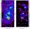 |
Fig. 1 Intensity of the far-infrared fine-structure lines [C II]λ158 µm (left) and [O III]λ88 µm (right) in W m−2 sr−1, observed by SOFIA/FIFI-LS. The intensities are the result of spectral Gaussian fits and only those fits with a S/N ≥ 3 are shown. Pixels with lower S/N are displayed as 0 (in black). The white contours are from LTIR (300 and 600 Lso//pc2) shown in Fig. 3. The thin black contours shown in the [C II] map are 8 µm from Spitzer/IRAC (4 and 8 MJy/Sr). The red contours in the [O III] map are Spitzer/MIPS 24 µm continuum (5 and 150 MJy/sr). The [C II] map is shown in the native resolution with a beam FWHM of 15.3″. The [O III] data in the three bright star formation regions marked by dashed blue, green and red lines was smoothed to the same resolution (15.3″) to increase the S/N per beam. Outside of the regions the data was further re-binned to 24″ and fit within a 48″ beam to further increase the S/N in the diffuse regions. The seven gray crosses, in identical positions in the [C II] and [O III] maps, mark the positions of the spectra shown in Appendix A. |
Observational parameters of SOFIA/FIFI-LS observations; the radial velocity was used to center the arrays spectrally and the beam size in parsecs was calculated based on a distance of 50 kpc; the integration time Tint is per FIFI-LS spatial pixel.
2 Observations and data reduction
2.1 SOFIA FIFI-LS
Observations of the [C II] and the [O III] lines were carried out with the Field-Imaging Far-Infrared Line Spectrometer (FIFI-LS) (Fischer et al. 2018; Colditz et al. 2018) on board SOFIA (Erickson & Davidson 1993; Young et al. 2012). FIFI-LS is an integral-field imaging spectrometer that provides simultaneous observations in two channels: the blue channel covering 51–125 µm and the red channel covering 115–203 µm. Each channel consists of an overlapping 5×5 pixel footprint on the sky, where the pixel size is 6″ and 12″ for the blue and red channels, respectively. We refer to each of these spatial pixels as “spaxels.” The optics within FIFI-LS rearranges the 25 spaxels into a pseudo-slit, and the light impinging on each spaxel is then dispersed spectrally (using a grating) over 16 pixels. This generates an integral-field data cube for each observation. The spectral resolution is wavelength dependent ranging from R = λ/∆λ = 500 to 2000.
2.1.1 Observations
SOFIA/FIFI-LS observations were taken in March 2022 as part of the Cycle 9 SOFIA Legacy Program, LMC+, 09_0036 (PIs S. Madden, A. Krabbe). SOFIA was on deployment to the southern sky flying out of Santiago de Chile. Of the awarded 20 h wall-clock time for the legacy project (50 h in total requested) 15 h were observed during 6 flights. While the metallicity of the Small Magellanic Cloud is even lower than that of the LMC, the line fluxes in the SMC that are a factor of two to four times lower (Cormier et al. 2015) would not have permitted a large map detecting [C II] in the lower brightness ISM conditions.
Due to the large size of the mapped region (~ 1º×0.5º), observations were performed without chopping in on-the-fly (OTF) mapping mode for maximum efficiency and best spatial sampling with short integration times per field. In this mode, the telescope scans across the mapping area at a constant speed. The speed (6″/s) was chosen to avoid distortion of the image during the shortest continuous integration, which is 0.125 s for FIFI-LS (Fischer et al. 2018). The movement of 0.75″ during this integration was less than 10% of the spatial FWHM at both observed wavelengths. The fine sampling provided by the scan enables mapping with the best possible spatial resolution (see Fadda et al. 2023) with the spatially oversized FIFI-LS pixels. With a scan length of 30s, 180″ were covered on the sky in one scan. With the field of view size of 30″ × 30″ in the blue channel, 12 scans were performed to fill the 3′ × 3′ tiles with 2×6 scans carried out in the perpendicular direction to ensure even sampling. The 5×5 spaxel array was tilted by 11.3º to spread out the spaxels evenly, perpendicular to the direction of the scan. At the beginning and the end of each scan, part of the 180″ scan was not seen by all of the spaxels. Full integration time there is reached by the overlap of the field of views with the scans from the neighboring tiles, creating an interlock.
With the 60″ × 60″ footprint of the red array, this mode produced additional overlap of the scans, resulting in a map with four times deeper integration, improved flat-fielding, and a uniformly deep integrated map. The efficiency (on-source integration time vs. wall clock time) was 51 %, well above the efficiencies achieved with pointed observations (Fischer et al. 2016). For background subtraction, a field with minimal expected [C II] emission1 as well as minimal 250 µm continuum emission2 was identified in proximity to the mapping region, ensuring an offset smaller than 30′ to all fields in the map. This allowed the telescope to reach the offset position within its limited movement range due to the aircraft’s orientation. Observational details for both lines are listed in Table 1. A more detailed description of the OTF observing mode with FIFI-LS is provided in Fischer et al. (2025).
The 3′×3′ interlocking tiles were the building blocks of each sub-map. The central region of the map with the three bright SFRs N158, N159, and N160, was covered in a single rectangular map with 14×6 tiles for a total extension of 42′×18′. Integrations were taken tile by tile in rows from the northern edge close to 30 Doradus and progressing southward. Originally, 7 flights were planned to complete all 84 tiles, with potential time for expansion further south. However, due to one lost flight, 76.25 tiles (91%) were completed. The relatively high completion rate was achieved through flight re-planning to maximize LMC leg times.
2.1.2 Data reduction
The data was reduced with the SOFIA/FIFI-LS pipeline (Vacca et al. 2020), which includes all the necessary calibrations and flat-field corrections (Fadda et al. 2023). We produced cubes with 6, 12 and 24 spatial pixel size for the analysis presented in this paper. Since OTF mapping mode was only offered for FIFI-LS on SOFIA since Cycle 9 and had never been used on a map of this large size, some modifications to the last SOFIA published version of the pipeline3 have been applied to achieve better background subtraction, noise propagation, and telluric correction.
We modified the noise calculation to better capture all noise contributions in OTF mode, i.e., nonlinear drifts of the telluric emission. While these are captured in pointed FIFI-LS observations by averaging ~50 data points (Fischer et al. 2016) with constant signal, this is not done for OTF where every data point on a scan has a different astronomical signal. Since the overall signal is background dominated, we can assume that any non-linear behavior of the signal on the scan is dominated by the background and not the astronomical emission. We introduced a new step in the data reduction procedure (“scan noise definition”) to quantify this for each scan and combined it with the errors for each data point. More details can be found in Fischer et al. (2025).
Due to the large size of the map, nod-offsets of up to ~30′ were required. Depending on the rotation of field of the SOFIA telescope, this can lead to significant changes in telescope elevation, which in turn affected the airmass. At the altitudes SOFIA operates (37 000–45 000 ft), the raw far-infrared signal is dominated by sky emission. As a result, the gradient in airmass during nodding for background subtraction can introduce significant signal, complicating the background subtraction process. This can also add noise to the baseline in the overlapping, interlocking region of the tiles. The signal offset due to imperfect back-ground subtraction varies over time, generating artifacts when tiles, taken at different times or even on different flights, over-lap. This effect can be amplified by telluric correction since this signal contributions are not transmitted through the atmosphere.
Two different approaches to remove artifacts from those air-mass differences were applied to the [C II] and [O III] data due to the different telluric features in the spectral ranges of the two lines. They are both described in full detail in Fischer et al. (2025). For [C II], a telluric scaling technique was used where an emission model with contributions from the atmosphere, as well as telescope and instrument background, is tend to the signal in each of the 25 spaxels in the off-nod. If there are significant telluric features in the spectral range, this two-component model allows the signal in each of the 400 pixels to be split up into the elevation-dependent sky emission and the background that is independent from the telescope elevation. The sky contribution, and with it the overall off-nod signal, were then scaled to the elevation of the on-nod. Telluric scaling was possible for [C II] but not for [O III], since there are no significant spectral features in the range used for the [O III] line. Thus, the telluric contribution to the [O III] signal cannot be quantified. Still, the spectra in the [O III] cube display underlying telluric artifacts. It has proven to be most advantageous to remove them during the fitting of the emission line described below.
For the telluric correction, we used water vapor values obtained with the method described in Fischer et al. (2021) and Iserlohe et al. (2021) in the pipeline. With the water vapor overburden, telescope elevation and flight altitude for each scan, a transmission profile is calculated with the ATRAN model (Lord 1992) for the observed spectral range. In the pipeline it is then spectrally smoothed to the instrument’s resolution and applied to each ramp at the observed wavelength in a background-subtracted nod pair. Using the smoothed transmission profiles does not distort the line profiles here since the transmission is spectrally flat in the relevant range in both channels. However, since we cannot remove baseline artifacts with telluric scaling for the [O III] map, we modified the telluric correction procedure in the pipeline to avoid further distortion of the baseline. For the [O III] map of the molecular ridge, the transmission of the emission line only depends on atmospheric conditions. It remains largely unaffected by variations in local velocity and line width. For each nod cycle, we determined the transmission at the wavelength of the [O III] line4 and applied this correction to the entire spectrum. This preserves the original baseline shape as measured. For the [O III] data, this approach enables telluric correction of the line flux based on the actual atmospheric conditions during the scan, while also allowing for the fitting of any residual telluric baseline.
2.1.3 [C II] and [O III] line fitting
The spectrally unresolved lines were ted in circular apertures around each spatial pixel with Gaussian profiles together with the baseline using a SciPy curve_fit function5. The line widths and center positions were constrained based on the spectral resolution of FIFI-LS (with margins) and the mapped region in the LMC (by multiple iterations of the fit). To avoid edge effects due to the re-binning, portions of the spectra near the spectral cube edges were cut. All fit parameters are listed in Table 2. For [C II], where telluric artifacts were removed using telluric scaling in the pipeline processing, a zero-order polynomial was tend to the baseline. For [O III], a residual telluric emission model was ted to the baseline. The model includes a zero-order polynomial and atmospheric transmission from ATRAN, which can be scaled positively or negatively to account for residual telluric emission caused by nodding to different elevations with the telescope. More details on this “telluric fitting” can be found in Fischer et al. (2025). Examples of line profiles and fits are shown in Appendix A.
The integrated line flux maps of [C II] and [O III] are shown in Fig. 1. The map of [C II] is shown in the native telescope resolution, with a FWHM of 15.3″ used as aperture diameter in the line fitting. The [O III] data was also fit with this aperture to improve the signal-to-noise ratio (S/N) per beam. They are shown together with the CO(2−1) line flux in Fig. 2. For the maps in Figs. 1 and 2, the data was spatially re-binned to 6″ and fit within 15.3″ diameter apertures around each spatial pixel for both [C II] and [O III]. It was increased to 24″ with a 48″ diameter apertures outside the bright star formation regions for [O III]. For all ratio plots the binning was increased to 12″ for [C II] and [O III] in the bright SFRs. The FΓFI-LS data was smoothed to 18″ resolution for ratio plots involving LTIR.
Fit parameters used for both lines of SOFIA/FΓFI-LS observations.
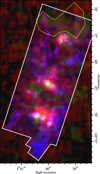 |
Fig. 2 RGB map of [C II] (r), [O III] (g) and 12CO(2−1) (b) from Tarantino et al. (in preparation) and Chen et al. (in preparation), with the map of the 12CO(2−1) outlined in white. Contours are shown for 12CO(2−1) line flux levels of 5 × 10¹¹ and 5 × 10¹⁰ Wm−2 sr−1. Regions for analyses in Sect. 4 are outlined, corresponding respectively to the SFRs, N159(green), N160(red), N158(blue), an extended, less active region in [O III] (yellow) and three CO-bright filaments (brown). They are also referred to in Fig. 3, and in the plots in Figs. 5 and 6. |
2.2 Cross calibration
A few bright regions of the LMC were observed with the Herschel Photodetector Array Camera and Spectrometer (PACS) (Cormier et al. 2015). This gave us the opportunity to cross calibrate the fluxes obtained with SOFIA/FIFI-LS. We were able to define 20 circular regions (12 for [C II] and 8 for [O III]) to perform such cross-correlation (see Table B.1). For each region we defined circular apertures with a 18″ radius. Such apertures were sufficiently larger than the PSF so that the measured fluxes were not affected by the spread of point-like emissions. Since the PACS data was obtained in “unchopped mode”, we reprocessed them using the “transient-correction” pipeline (see Fadda et al. (2016) and Sutter & Fadda (2022a) for recent updates). In fact, as pointed out in Fadda et al. (2023), the PACS data in the Herschel Science Archive can deviate significantly since the flux calibration was based on the internal calibrators rather than on the more stable telescope background as is the case of normal chop-nod observations. Sudden flux changes when switching between source and internal calibrators can induce a major, unpredictable transient in the signal, varying the response of the detectors up to 90%. The fluxes were evaluated with pseudo-Voigt curves which provide the best fitting and recover most of the flux in the wings of the spectra for the higher S/N in the PACS spectra (see Fadda et al. 2023). With an average deviation below 5% (3% for [C II] and 4.6% for [O III]), the agreement between FΓFI-LS and PACS data is excellent and well within the estimated flux uncertainties of PACS and FΓFI-LS (Exter 2019; Fadda et al. 2023).
2.3 Ancillary data
2.3.1 ALMA CO(2−1)
To map the molecular ridge in CO(2−1) as a tracer of molecular gas it was observed with the Atacama Large Millimeter/Submillimeter Array (ALMA) Atacama Compact Array (ACA), also known as the Morita array. These observations were part of Cycle 7, under project code 2018.A.00061.S (PI: Bolatto, A). The map covers a region of 10′ × 26′ (150 pc × 380 pc) across the northern tip of the molecular ridge in the LMC, over-lapping with three H II regions: N158, N160, and N159 and the majority of the SOFIA observations. The map is comprised of sixteen individual 10′ × 2.3′ tiles. One frequency setting was configured to cover the 12CO(2−1) line at 230.538 GHz with a bandwidth of 125 MHz and a channel width of 61 kHz. The second frequency setting covered both 13CO(2−1) at 220.399 GHz and C18O(2−1) at 219.560 GHz with bandwidths of 62.5 MHz and a channel width of 61 kHz. We also included a broader continuum frequency set-up centered at 232.6 GHz with a bandwidth of 2 GHz. These observations include total power ALMA data corresponding to the full rectangular region covering the interferometric map produced on October 15th, 2019, providing short spacings information.
We used version 6.5.1 of the Common Astronomy Software Applications (CASA Team 2022) and the standard system calibration to image the molecular ridge data. We imaged each of the sixteen individual tiles that comprise the final map separately and stitched them together to create the final mosaic. Imaging each tile separately provides higher stability and convergence in the de-convolution algorithm (see also Leroy et al. 2021). For the spectral line data, we used the CASA task sdint to image and combine the ACA and TP data. The sdint algorithm is a joint de-convolution algorithm that simultaneously images and combines interferometric and single dish data (Rau et al. 2019). We found that the sdint algorithm produces better results than the traditional tclean and feather method. Each tile has a square pixel cell size of 1.2″, a velocity channel of 0.25 km s−1, and a total size of 600 × 300 pixels. We chose 320 channels which corresponds to the maximum size of the bandwidth for the 13CO(2−1) and C18O(2−1) data. We used a cleaning threshold of 0.3 Jy/beam and a cyclefactor = 5 in order to make sure the cleaning algorithm does not diverge before it reaches the threshold. We used the mosaic gridder, hogbom deconvolver, and Briggs weighting with robust = 0.5, which provides the best combination of resolution and signal-to-noise. We masked the data for cleaning through the auto-multithresh and the default parameters. The interferometric data was combined with the total power data using an sdgain = 3, which preserves the flux information from the total power data while maintaining the high resolution structure. We convolved the data cubes to a common restoring beam of 7″ (1.7 pc). The details of the reduction and analysis of the 12CO(2−1), 13CO(2−1), and C18O(2−1) will be presented in Tarantino et al., in prep.
The ACA CO(2−1) observations of N159’s southern region were obtained as part of the ALMA project 2016.1.00782.S (PI: Chen, R.). The map is comprised of two rectangle regions, 96″×200″+78″×50″(23 pc×49 pc+20 pc×12 pc) that covers all bright CO filaments detected in the Atacama Pathfinder Experiment (APEX) CO(2″1) mosaic (under project ID M-092.F-0020). The Band 6 receiver setup for the CO(2−1) line has a bandwidth of 117.2 MHz and a channel width of 141 kHz (or 0.184 km s−1); the receiver setup and detailed reduction and analysis for other lines in Band 6 including 13CO(2−1), C18O(2−1), SİO(5−4), H2CO(30,3−30,2, 32,2−32,1, 32,1−32,0), 13CS(5−4) will be presented in Chen et al. (in prep.). The ACA observations do not include total power ALMA data as the APEX CO(2−1) mosaic is available for the short spacing information. The ACA and APEX CO(2-1) data were combined using the feather task under CASA.
2.3.2 The total infrared map
The map of the Total InfraRed (TIR; 3–1000 µm) power in our region was computed from its spatially resolved spectral energy distribution (SED). The dust parameter maps derived from this SED modeling are presented by Belloir et al. (in preparation) using the Spitzer Infrared Array Camera (IRAC) and Multi-band Imaging Photometer for Spitzer (MIPS) maps at λ=3.6, 4.5, 5.8, 8.0, 24 and 70 µm from the SAGE project (Meixner et al. 2006) and the Herschel/PACS and the Spectral and Photometric Imaging Receiver (SPIRE) maps λ=100, 160, 250 µm from the HERITAGE project (Meixner et al. 2013). The angular resolutions of these maps were homogenized to 18″ using the convolution kernels of Aniano et al. (2011) and re-projected onto the SOFIA [C II] pixel grid. The noise uncertainties of the original maps were propagated through the homogenization process using a bootstrapping method (Press et al. 2007). At the end of this process a spectral cube (RA, Dec, λ) and its corresponding noise cube were obtained. The homogenized spectral cube was then fit using the hierarchical Bayesian code, HerBIE (Galliano 2018). The model set-up was identical to that used by Galliano et al. (2021): a dust mixture, with the properties of the THEMIS dust model (Jones et al. 2017), illuminated by a range of starlight intensities, U, following a power-law distribution and a stellar continuum, approximated as the Rayleigh-Jeans tail of a black body. HerBIE accounts for the fact that calibration uncertainties are spatially fully correlated and spectrally partially correlated. The hierarchical Bayesian approach of this model provides a regularization of the pixels with poor signal-to-noise ratios. The most relevant inferred parameters, for each pixel, are (see Galliano 2018; Galliano et al. 2021):
the total dust mass, Mdust;
the fraction of small amorphous carbon grains, carrying the mid-IR aromatic features, qAF;
the mean starlight intensity, 〈U〉;
the TIR luminosity, LTIR (Figure 3).
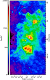 |
Fig. 3 Map of TIR power in the molecular ridge. Regions for the analyses in Section 4 are outlined, corresponding, respectively, to the SFRs, N159 (green), N160 (dotted red), N158 (blue), an extended, less active region in [O III] (yellow), and three CO-bright filaments (dashed brown). They are also shown in Fig. 2, and used in the plots in Figs. 5, 4, and 6. |
2.3.3 Spitzer MIPS and MCELS Hα
The Spitzer/MIPS 24 µm data for the molecular ridge were available on the IRSA Infrared Science Archive6. The Hα data were from the Magellanic Cloud Emission-line Survey (MCELS, Points et al. 2024) available at the NOIRLab Astro Data Archive7. They are used as tracers of exposed (Hα) and embedded (24 µm) star formation in comparison with the [O III] data to investigate the distribution of the dust and gas densities, the role of the excitation sources and radiation field and the porosity.
3 Results
3.1 [C II] emission
[C II] is detected with S/N ≥ 3 almost everywhere in the mapped region (Fig. 1). The highest fluxes are observed toward the three bright SFRs, but there is also significant diffuse emission throughout the mapped region, especially compared to LTIR, which drops off steeply beyond the SFRs (Fig. 3). The good correlation of [C II] with the 8 µm continuum observed toward the bright SFRs by Okada et al. (2019a) is also obvious in our map and holds as well for the extended structures shown by the black 8 µm contours in Fig. 1. The spatial correlation between the [C II] emission and 8 µm emission is seen even for the low [CII] fluxes (values < 3 × 10⁻⁷ W m−2 sr−1), except in the northern and western parts of the map, where [C II] emission is more extended than the 8 µm emission. Comparison of the [C II] map to the distribution of CO(2−1), shows that the SFRs are bright in both tracers, as expected (and in [O III], as well). In the more diffuse regions, well beyond the star-forming sites, however, there is no recognizable correlation spatially between [C II] and CO(2−1). Fig. 2 also shows how diffuse the [C II] emission compares to the filamentary structure of the CO(2−1) emission.
3.2 [O III] emission
While [C II] emission is well detected almost everywhere in the mapped region, [O III] is more challenging to detect. This is mainly due to the higher noise level of the [O III] map caused by the smaller integration time per beam of the blue channel. To analyze the data, we smoothed the map to the same resolution as [C II] in the three bright star formation regions (15.3″). However, to increase the S/N per beam everywhere else in the map, the map was re-binned to 24″ with a 48″ aperture for the line fits (Fig. 1) there. The resulting map shows that the [O III] emission, which traces ionized gas, is more localized and compact compared to the [C II] emission. The brightest [O III] emission is concentrated toward the three major SFRs, dropping off rapidly beyond the star-forming sites. Yet, [O III] emission is still detected in large areas of the map even outside of the bright regions. This is consistent with the detections of [O III] by AKARI in the molecular ridge region Kawada et al. (2011). Where [O III] is detected, it is typically brighter than [C II] (see Fig. 5). The bright [O III] emission spatially correlates with the 24 µm emission and with the LTIR which are usually attributed to dust heating by young, massive stars and serve as a good tracers of ongoing dust-obscured star formation (e.g., Gratier et al. 2012; Corbelli et al. 2017; Kim et al. 2021). Notably, there is an extended region directly north of N158 (marked in yellow in Figs. 2 and 3), which has extended clear detections of [O III], although not particularly bright in [C II] or LTIR.
4 Discussion
In this section, we investigate the relationship between [C II] and [O III], and other tracers to characterize the physical properties of the region. Due to the ionization potential of carbon being close to but smaller than that of hydrogen, [C II] can trace gas from H II regions as well as PDRs. Studies have shown that the ionized phase often contributes negligibly to its emission (e.g., Pineda et al. 2013; Tarantino et al. 2021). In particular, in low-Z environments [CII] originates predominantly from PDRs rather than from H II regions (Cormier et al. 2019; Lebouteiller et al. 2019; Ramambason et al. 2022). In general, any [C II] arising from the ionized gas decreases as the radiation field increases. Toward 30 Doradus, one of the most massive SFRs in the LMC, it has been shown that at least 90% of the [C II] emission originates in PDRs (Chevance et al. 2016). To aid in the interpretation of the ratio plots, we highlight several regions, which are shown in the three-color image in Fig. 2 and the LTIR image of Fig. 3. The three bright SFRs, N158 (blue), N160 (red), and N159 (green), were delineated by hand based on the LTIR emission (Fig. 3) at a level of ~1000 Lsol/pc2. Some regions based on bright CO(2−1) emission relative to LTIR are outlined in brown and a region of relatively bright diffuse [O III] emission, located north of N158, is outlined in yellow. These regions are noted in these colors in the plots of Figs. 4, 5 and 6.
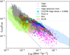 |
Fig. 4 L[C II]/LTIR versus LTIR in the molecular ridge in 12″× 12″ pixels. Yellow, blue, red, green, and brown colors refer to the regions outlined in Figs. 2 and 3. Gray points represent the pixels in the ridge outside of these regions. Data for 30 Doradus from Chevance et al. (2020) is added. The gray line represents the average minimum detectable [C II] line flux for S/N = 3. The large circles represent the ratio values for the whole ridge (cyan) and the three bright SFRs (N158: blue; N160: red; Nl59:green), relative to the mean LTIR. The areas with filled colors represent observations from: Orion A (Pabst et al. 2021); M51 (Pineda et al. 2018); N11B (Lebouteiller et al. 2012). |
4.1 [C II] compared to TIR
In conditions of thermal equilibrium within PDRs, the heating due to the radiation from young stars should be balanced by the cooling through line emission. Dust absorbs UV radiation emitted by stars, and primarily cools by re-emitting in the infrared. Small grains and polycyclic aromatic hydrocarbons (PAHs), when heated by stellar radiation, release electrons that heat the surrounding gas, via the process of photoelectric heating – the dominant heating mechanism in PDRs (see e.g., review by Wolfire et al. 2022). The fraction of energy in the dust heating that is transferred to the gas heating is measured with the photoelectric heating efficiency, which is the ratio of gas heating to dust heating. Since [C II] emission is the main cooling channel in diffuse PDRs, and LTIR accounts for all contributions from the dust emission, the L[C II]/LTIR ratio has been used as a tracer of the photoelectric heating efficiency (e.g., Diaz-Santos et al. 2013; Cormier et al. 2015). Several studies (e.g., Malhotra et al. 1997; Graciá-Carpio et al. 2011; Diaz-Santos et al. 2017; Herrera-Camus et al. 2018) have shown that the L[C II]/LTIR ratio decreases with the increase in LTIR for emission integrated over full galaxies. This “[C II]-deficit” affects the reliability of [C II] as a tracer of star formation. Herrera-Camus et al. (2018) investigated the [C II]-deficit in a sample of unresolved galaxies using toy models as well as Cloudy simulations. Their findings suggest that the observed decrease in L[C II]/LFIR can be explained by an increase in the ionization parameter with LFIR. The models indicate that as the ionization parameter increases, the far-infrared emission increases, but the photoelectric heating efficiency declines, leading to a reduction in L[C II]/LFIT. Several recent studies using higher spatial resolution data from Herschel and SOFIA resolving parts of galaxies or fully mapping them (e.g., Lutz et al. 2016; Smith et al. 2017; Pineda et al. 2018; Bigiel et al. 2020; Sutter & Fadda 2022b) have shown that the [C II] deficit is not driven by global properties of galaxies but rather by local physical properties. These studies find that the L[C II] to LTIR ratio continuously declines with increasing LTIR. A similar trend was also shown within the Milky Way with a large-scale [C II] map in Orion A by Pabst et al. (2021), confirming this behavior.
Figure 4 shows the L[C II]/LTIR ratio as a function of LTIR (Belloir et al., in preparation) for the molecular ridge as well as 30 Doradus (Chevance et al. 2020). The L[C II]/LTIR ratio for the entire molecular ridge is about 0.7% and the three bright SFRs with around 0.3% fall well within the range for entire galaxies in the DGS sample (0.04%–0.8%) from Cormier et al. (2015). The values throughout the molecular ridge span about three orders of magnitude in LTIR and about two orders of magnitude in the L[C II]/LTIR ratio, with a clear trend of decreasing L[C II]/LTIR as LTIR increases. The ridge regions extended beyond the main SFRs (gray points in Fig. 4) are located in the upper left of the plot, exhibiting the highest L[C II]/LTIR ratios and lowest LTIR values, followed by the regions with bright CO(2−1) emission (brown) and regions with relatively bright diffuse [O III] emission (yellow) located outside the main SFRs, north of N158. Next in the sequence are the data of the SFRs of the ridge, which in parts are bright in LTIR and overlap with the 30 Doradus data points, that show very low L[C II]/LTIR with high LTIR.
Throughout the molecular ridge, L[C II]/LTIR maintains a clear trend, with less scatter than in 30 Doradus, varying by no more than ~0.5 orders of magnitude from a straight trend. At lower LTIR, the trend is potentially affected by the noise limit of the [C II] map, but remains clear, as [C II] is detected in the large majority of the mapping area. The three brightest SFRs exhibit a pronounced decline in L[C II]/LTIR in their brightest regions, compared to the overall trend. In these dense regions, [O I] line emission likely contributes significantly to the cooling (as seen in N11 in Lebouteiller et al. 2012). However, the clear and continuous drop in L[C II] relative to LTIR throughout the dynamic range strongly suggests a correlated decrease in the photoelectric heating efficiency with increasing LTIR.
For the bright SFRs, LTIR spans a similar range to that in the 30 Doradus map. The L[C II]/LTIR ratio falls into the same range as in 30 Doradus. However, for most of the data points of 30 Doradus, the L[C II]/LTIR ratio is lower than in any part of the molecular ridge. The ionizing sources in 30 Doradus, which are more energetic than those of N158, N159, and N160, lead to increased ionization of carbon ions, reducing [C II] emission relative to LTIR (Chevance et al. 2016).
At lower spatial resolution, Israel et al. (1996) observed enhanced [C II] emission relative to infrared emission around N159, attributing it to deep UV penetration due to low dust-to-gas ratio. Similarly, Madden et al. (1997) encountered elevated L[C II]/LTIR in some more diffuse regions of the low-Z galaxy IC10, suggesting that the high ratio indicates the presence of low UV fields and deep UV penetration caused by the low dust-to-gas ratio. This also is thought to result in a large fraction of CO-dark molecular gas in those regions where [C II] presumably is tracing significant amounts of molecular hydrogen. The trend also agrees with the findings in M33 by Kramer et al. (2020), where a different LTIR definition was used, preventing a precise comparison.
Figure 4 also displays the range of values from N11B (Lebouteiller et al. 2012) in the LMC, as well as large regions mapped in Orion A (Pabst et al. 2021), and M51 (Pineda et al. 2018). The spread of values altogether show good agreement, following the sequence the ridge observations, across different environments and scales, revealing a consistent trend: L[C II]/LTIR increases at lower LTIR values, with a tight correlation. This suggests a strong link between the [C II]-deficit and local physical conditions. A more detailed analysis of the L[C II]/LTIR ratio and possible origins of the high values found in the diffuse parts of the ridge is presented in Belloir et al. (in preparation).
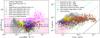 |
Fig. 5 Line ratio plots for the molecular ridge. Yellow, blue, red, green, and brown colors refer to the regions outlined in Figs. 2 and 3. Gray points represent the pixels in the ridge outside of these identified regions. Left: L[O III]/L[C II] versus LTIR in 12″ pixels for the three bright star formation regions and in 24″ pixels for the rest of the molecular ridge, where pixels with S/N below 5 are shown as upper limits. 30 Doradus data points from Chevance et al. (2020) have been added with 12″ binning. The horizontal lines show the mean L[O III]/L[O II] ratio for the regions. Right: L[O II]/LTIR versus L[CO]/LTIR in 12″ pixels. CO(1−0) was estimated from CO(2−1) assuming a ratio of CO(2−1)/CO(1−0) of 0.6 (e.g., den Brok et al. 2021; Maeda et al. 2022). The average ratio (no fit) of L[C II]/LCO(1−0) from the molecular ridge is indicated with the cyan line. The large circles represent the ratios based on the fluxes for the whole regions, in cyan for the whole molecular ridge and in matching colors for the three star formation regions. The area filled in red represents the data range for dwarf galaxies from Madden et al. (2020) using a LTIR to LFIR ratio of 0.6. |
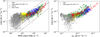 |
Fig. 6 [O III] emission versus 24 µm continuum emission (left) and versus Hα (right) in the three star formation regions in 12″ × 12″ pixels and at 48″ resolution (in 24″ × 24″ pixels) for the rest of molecular ridge map with a detection more than 5σ in both. Yellow, blue, red and green colors refer to the regions outlined in Figs. 2 and 3. Gray points represent the pixels in the ridge outside of these identified regions. For the diffuse regions shown in gray and yellow, fit results with a S/N below 5 are shown as upper limits. The black lines in the left plot show the fit linear relation and the 95% confidence interval from Lambert-Huyghe et al. (2022). |
4.2 [O III] compared to [C II]
The ratio of L[O III]/L[C II] over LTIR is shown in Fig. 5 left. For comparison, data for 30 Doradus from Chevance et al. (2020) are shown as well. In the diffuse regions, we display pixels with S/N > 5 for both emission lines, while pixels with lower S/N are also included but marked with different symbols. The range of ratios observed closely matches the range of ratios integrated over the low-Z dwarf galaxies from the DGS sample (Cormier et al. 2015). While [O III] line flux is on average 13 times that of [C II] in the 30 Doradus map, the values are significantly lower in the SFRs along the molecular ridge. The L[O III]/L[C II] ratio is on average 3.2 for N158 and 2.3 for N160 and 2.2 for N159 – consistent with these regions being less energetic than 30 Doradus. The three bright SFRs exhibit a wide range of L[O III]/L[C II] ratios. In some areas, the ratio is particularly low because the [O III] emission declines sharply beyond the H II regions, where the ionizing radiation is less energetic and conditions are less favorable for producing [O III] emission, due to its relatively high ionization potential of ~35 eV.
The remaining points, corresponding to more diffuse emission (yellow, brown, and gray), generally exhibit higher L[O III]/L[C II] ratios, with a trend of increasing ratios at lower LTIR values. Due to the limited area where [O III] has been detected, this does not show a general trend but rather the existence of areas in the diffuse parts of the molecular ridge with relatively high L[O III]/L[C II] compared to the bright star formation regions. The [O III] emission of these areas is, on average, 4.1 times stronger than the [C II] emission. Lower ratios are expected in the regions without clear detections as shown by the ratios based on the upper limits for [O III]. Similar to 30 Doradus (Chevance et al. 2020), the existence of relatively strong [O III] detections compared to [C II] in the extended, diffuse regions of the molecular ridge, indicates the high porosity of the low-Z environment, where high energy photons can travel significant distances before interacting with the ISM. The L[O III]/L[C II] ratio is higher in the more diffuse regions, where L[C II]/LTIR is elevated as well, also suggesting the presence of a diffuse UV field permeating a porous, clumpy ISM. This is further supported by the small-scale clumpy structure observed in the CO(2−1) map (Section 4.3). This conclusion is in agreement with those of Poglitsch et al. (1995) and Chevance et al. (2016) for 30 Doradus and Lebouteiller et al. (2012) for N11B.
4.3 [C II] compared to CO
The L[C II]/LCO(1−0) ratio has been used as a tracer of global star formation activity in galaxies (e.g., Stacey et al. 1991). In normal star-forming galaxies this ratio typically ranges from ~1000 to 4000, with higher values observed in more active starburst galaxies (e.g., Stacey et al. 1991; Stacey et al. 2010; Hailey-Dunsheath et al. 2010). In contrast, dwarf galaxies show ratios as high as 80 000 (Madden et al. 2020).
Figure 5 right shows the [C II] luminosity versus the CO luminosity (where both [C II] and CO(2−1) have been detected) normalized by LTIR. To estimate the CO(1−0) luminosity we used the CO(2−1) ALMA data from Tarantino et al. (in preparation) and Chen et al. (in preparation) and assumed a CO(2−1)/CO(1−0) ratio of 0.6 in K/(km/s) (e.g., den Brok et al. 2021; Maeda et al. 2022). [C II] is much more extended and diffuse than CO, which leads to a large range of L[C II]/LCO(1−0) across the map, from 300 to over 100 000. While both [C II] and CO peak locally on the LTIR peaks, CO exhibits filamentary structures not associated with either [C II] or LTIR emission and [C II] is present where no CO exists, as well. Some of these regions, framed in brown in Fig. 2, show large variations in L[CO]/LTIR and L[C II]/LCO(1−0) (300–25 000) ratio as well as the highest L[CO]/LTIR and the lowest L[C II]/LCO(1−0) values. Even within the three bright SFRs, the L[C II]/LCO(1−0) ratios vary significantly, from about 1000 up to over 100 000. The average ratios of the SFRs, N158 (17 000), N160 (12 000), and N159 (8000) closely match the overall molecular ridge average value of 11 000. When computed pixel by pixel, the average ratio is even higher (25 500), with a tendency toward higher ratios in the more diffuse areas.
While the L[C II]/LCO(1−0) ratios in the molecular ridge (300 to 100 000) are lower compared to those found in 30 Doradus (50 000–200 0000 (Chevance et al. 2016)), they are very high compared to normal star-forming galaxies(1000–4000). Both the molecular ridge overall, as well as the three SFRs, exhibit values of L[C II]/LCO(1−0) ( as well as L[C II]/LTIR and L[CO]/LTIR) typical of the ratios integrated over the low-Z galaxies from the DGS sample (Cormier et al. 2015; Madden et al. 2020; Ramambason et al. 2024). The extreme range of L[C II]/LCO(1−0) ratios in the molecular ridge reflects significant variations in CO emission. The L[CO]/LTIR ratios span more than two orders of magnitude, the spread being driven, for the most part, by variations in CO, rather than variations in LTIR. Across the map, L[C II]/LCO(1−0) values vary by three orders of magnitude, with higher ratios in regions with low LCO, holding important implications for CO-dark gas as well as the multiphase nature of [C II]. This will be explored further in an upcoming paper.
4.4 [O III] compared to 24 µm continuum emission
Lambert-Huyghe et al. (2022) demonstrated a correlation between [O III] emission and 24 µm continuum emission using spatially resolved Herschel/PACS [O III] maps of SFRs throughout the LMC. While Lambert-Huyghe et al. (2022) include N158, N159, and N160 in their study, the [O III] observations were limited strictly to the bright star formation sites, not going beyond. Their study also included the unresolved galaxy-wide low-Z DGS galaxies. While [O III] traces the ionized gas, the ~24 µm continuum emission is emitted, for the most part, by the warm dust and is considered to be one of the most reliable tracers of the star formation rate in galaxies (e.g., Kennicutt et al. 2009, Whitcomb et al. 2023, Belfiore et al. 2023). With the new data presented in this paper, we extend the analysis of Lambert-Huyghe et al. (2022) to the surrounding medium beyond the previously targeted SFRs only, investigating the behavior of the 24 µm warm dust and the [O III] in the more extended, diffuse, low-Z environments.
Figure 6 shows that the [O III] line emission and the 24 µm continuum emission correlate well within the three bright SFRs, beyond the small areas of peak [O III] emission mapped with Herschel/PACS, and, in general, follow the correlation shown by Lambert-Huyghe et al. (2022) and also seen in some LMC regions detected by AKARI (Kawada et al. 2011)8. However, in the more extended, diffuse regions (gray and yellow markers), where the 24 µm emission has fallen off and [O III] remains well-detected, we find a deviation from the rather tight correlation of [O III] and 24 µm toward the bright star formation sites. The [O III] − 24 µm relation has a tendency to flatten further from the star-formation sites. [O III] emission can exist, where the hot dust emission arising from 24 µm does not reach. The dust and the highly excited [O III] seem to be well mixed around the SFRs, but less so outside these regions.
Related to this, we do see a correlation between [O III] and Hα (Fig. 6) for the brighter SFRs as well. For lower values of Hα, [O III] is also relatively more prominent, pointing to a flattening out of the correlation seen for higher values of H α, similar to [O III] versus 24 µm. Overall, the individual SFRs and the extended regions have different behaviors in [O III] versus 24 µm and [O III] versus Hα (and [O III] versus [C II]; see Section 4.2). This will be the subject of a follow-up study to investigate the roles of the excitation sources and radiation field, the distribution of dust and gas densities, and porosity in the observations.
5 Conclusions
The SOFIA Legacy Project, LMC+, has mapped a 610pc × 260pc region in the molecular ridge in the LMC in [C II] and [O III] at 2.5 pc resolution, using FIFI-LS. This paper presents the first results from these observations, including the line flux maps, details of the observational strategy and the data reduction procedures, for which some new techniques have been developed. Both the [C II]λ158 µm and [O III]λ88 µm lines are detected widespread throughout the region. This first analysis compares the LMC+ observations with maps of other tracers, including CO(2−1) from ALMA (Tarantino et al., in preparation; Chen et al., in preparation), Spitzer 24 µm, and LTIR (Belloir et al., in preparation). We summarize our findings here:
While the [C II] emission peaks toward the three prominent star-forming sites, N158, N159, and N160, it is detected well beyond these concentrations, throughout the LMC+ map. The importance of [C II] as a cooling line relative to LTIR increases with decreasing LTIR. Across a wide variety of environments and different size scales, we see a consistent, tight correlation between L[C II]/LTIR and LTIR over three orders of magnitude of LTIR, with increasingly high values of L[CII]/LTIR for lower values of LTIR. This trend points to a strong link between the [C II]-deficit and the local physical conditions instead of global properties.
We find extended bright [O III] emission throughout the region, even beyond the three bright star formation regions. Where [O III] is detected, it is almost always brighter than [C II]. The L[O III]/L[C II] ratio reaches 10 in the extended, more diffuse regions, indicating the presence of a diffuse UV field within a porous and clumpy ISM. However, the ridge values of L[O III]/L[C II] do not reach the extreme ratios of ~100 found in 30 Doradus (Chevance et al. 2020).
We find the L[C II]/LCO(1−0) ratio to be extremely high in most of the molecular ridge as well to display a large variation of over three orders of magnitude with high L[C II]/LCO(1−0) preferring regions with low LCO, possibly holding important implications for CO-dark gas.
We confirm the correlation between [O III] and 24 µm found by Lambert-Huyghe et al. (2022) who targeted only the bright SFRs. Where we detect [O III] emission outside of the brightest regions, it is not correlated with 24 µm, but remains high as the 24 µm emission decreases, another indication of the high porosity of the ISM in this environment.
This paper presents the first results of the LMC+ project, with the aim of characterizing the physical conditions and thermal processes across the different phases of the ISM. By zooming into our nearest low-Z galaxy, an ideal laboratory for such studies, we can understand how local ISM properties influence star formation on parsec scales. Future papers will provide detailed modeling and analyses to further explore these goals.
Data availability
Line flux maps of [C II] and [O III] are available at the CDS via https://cdsarc.cds.unistra.fr/viz-bin/cat/J/A+A/702/A273.
Acknowledgements
We acknowledge the dedication of the whole SOFIA 2022 Chile deployment team and the local staff in Santiago de Chile to making the SOFIA observations happen under the challenging boundary conditions of the flight series. We also thank the anonymous referee for the useful and constructive comments and suggestions, which helped improve the clarity and quality of the manuscript. SOFIA, the “Stratospheric Observatory for Infrared Astronomy” is a joint project of the Deutsches Zentrum für Luft-und Raumfahrt e.V. (DLR, German Aerospace Centre; grants 50OK0901, 50OK1301 and 50OK1701) and the National Aeronautics and Space Administration (NASA). This paper makes use of the following ALMA data: ADS/JAO.ALMA#2018.A.00061.S. ALMA is a partnership of ESO (representing its member states), NSF (USA) and NINS (Japan), together with NRC (Canada), NSTC and ASIAA (Taiwan), and KASI (Republic of Korea), in cooperation with the Republic of Chile. The Joint ALMA Observatory is operated by ESO, AUI/NRAO and NAOJ. It is funded on behalf of DLR by the Federal Ministry for Economic Affairs and Energy based on legislation by the German Parliament and funded by the state of Baden-Württemberg and the Universität Stuttgart. Scientific operation for Germany is coordinated by the German SOFIA Institute (DSI) of the Universität Stuttgart, in the USA by the Universities Space Research Association (USRA). Part of this work has been funded by the NASA grant number 09_0036. MC and LR gratefully acknowledge funding from the DFG through an Emmy Noether Research Group (grant number CH2137/1-1). COOL Research DAO (Chevance et al. 2025) is a Decentralized Autonomous Organization supporting research in astrophysics. MR wishes to acknowledge partial support from ANID(CHILE) through Basal FB210003. T.W. acknowledges financial support from the University of Illinois Vermilion River Fund for Astronomical Research. FG acknowledges support by the French National Research Agency under the contracts WIDENING (ANR-23-ESDIR-0004) and REDEEMING (ANR-24-CE31-2530), as well as by the Actions Thématiques “Physique et Chimie du Milieu Interstellaire” (PCMI) of CNRS/INSU, with INC and INP, and “Cosmologie et Galaxies” (ATCG) of CNRS/INSU, with INP and IN2P3, both programs being co-funded by CEA and CNES.
References
- Aniano, G., Draine, B. T., Gordon, K. D., & Sandstrom, K. 2011, PASP, 123, 1218 [Google Scholar]
- Belfiore, F., Leroy, A. K., Williams, T. G., et al. 2023, A&A, 678, A129 [NASA ADS] [CrossRef] [EDP Sciences] [Google Scholar]
- Bigiel, F., de Looze, I., Krabbe, A., et al. 2020, ApJ, 903, 30 [CrossRef] [Google Scholar]
- Bolatto, A. D., Wolfire, M., & Leroy, A. K. 2013, ARA&A, 51, 207 [CrossRef] [Google Scholar]
- Boreiko, R. T., & Betz, A. L. 1991, ApJ, 380, L27 [Google Scholar]
- Bouwens, R. J., Smit, R., Schouws, S., et al. 2022, ApJ, 931, 160 [NASA ADS] [CrossRef] [Google Scholar]
- CASA Team (Bean, B., et al.) 2022, PASP, 134, 114501 [NASA ADS] [CrossRef] [Google Scholar]
- Chevance, M., Madden, S. C., Lebouteiller, V., et al. 2016, A&A, 590, A36 [NASA ADS] [CrossRef] [EDP Sciences] [Google Scholar]
- Chevance, M., Madden, S. C., Fischer, C., et al. 2020, MNRAS, 494, 5279 [Google Scholar]
- Chevance, M., Kruijssen, J. M. D., & Longmore, S. N. 2025, arXiv e-prints [arXiv:2501.13160] [Google Scholar]
- Chruslinska, M., & Nelemans, G. 2019, MNRAS, 488, 5300 [NASA ADS] [Google Scholar]
- Cohen, R. S., Dame, T. M., Garay, G., et al. 1988, ApJ, 331, L95 [Google Scholar]
- Colditz, S., Beckmann, S., Bryant, A., et al. 2018, JAI, 7, 1840004 [Google Scholar]
- Corbelli, E., Braine, J., Bandiera, R., et al. 2017, A&A, 601, A146 [NASA ADS] [CrossRef] [EDP Sciences] [Google Scholar]
- Cormier, D., Madden, S. C., Lebouteiller, V., et al. 2014, A&A, 564, A121 [NASA ADS] [CrossRef] [EDP Sciences] [Google Scholar]
- Cormier, D., Madden, S. C., Lebouteiller, V., et al. 2015, A&A, 578, A53 [CrossRef] [EDP Sciences] [Google Scholar]
- Cormier, D., Abel, N. P., Hony, S., et al. 2019, A&A, 626, A23 [NASA ADS] [CrossRef] [EDP Sciences] [Google Scholar]
- De Looze, I., Cormier, D., Lebouteiller, V., et al. 2014, A&A, 568, A62 [NASA ADS] [CrossRef] [EDP Sciences] [Google Scholar]
- den Brok, J. S., Chatzigiannakis, D., Bigiel, F., et al. 2021, MNRAS, 504, 3221 [NASA ADS] [CrossRef] [Google Scholar]
- Díaz-Santos, T., Armus, L., Charmandaris, V., et al. 2013, ApJ, 774, 68 [Google Scholar]
- Díaz-Santos, T., Armus, L., Charmandaris, V., et al. 2017, ApJ, 846, 32 [Google Scholar]
- Erickson, E. F., & Davidson, J. A. 1993, Adv. Space Res., 13, 549 [Google Scholar]
- Exter, K. 2019, Quick-start guide to Herschel-Pacs the spectrometer, version 1.3 [Google Scholar]
- Fadda, D., Jacobson, J. D., & Appleton, P. N. 2016, A&A, 594, A90 [NASA ADS] [CrossRef] [EDP Sciences] [Google Scholar]
- Fadda, D., Colditz, S., Fischer, C., et al. 2023, AJ, 166, 237 [NASA ADS] [CrossRef] [Google Scholar]
- Finn, M. K., Indebetouw, R., Johnson, K. E., et al. 2021, ApJ, 917, 106 [NASA ADS] [CrossRef] [Google Scholar]
- Fischer, C., Bryant, A., Beckmann, S., et al. 2016, in SPIE Conference Series, 9910, Observatory Operations: Strategies, Processes, and Systems VI, 991027 [Google Scholar]
- Fischer, C., Beckmann, S., Bryant, A., et al. 2018, JAI, 7, 1840003 [Google Scholar]
- Fischer, C., Iserlohe, C., Vacca, W., et al. 2021, PASP, 133, 055001 [NASA ADS] [CrossRef] [Google Scholar]
- Fischer, C., Fischer, N., Vacca, W., et al. 2025, PASP, 137, 075002 [Google Scholar]
- Fukui, Y., Kawamura, A., Minamidani, T., et al. 2008, ApJS, 178, 56 [Google Scholar]
- Fukui, Y., Harada, R., Tokuda, K., et al. 2015, ApJ, 807, L4 [NASA ADS] [CrossRef] [Google Scholar]
- Fukui, Y., Tokuda, K., Saigo, K., et al. 2019, ApJ, 886, 14 [NASA ADS] [CrossRef] [Google Scholar]
- Galliano, F. 2018, MNRAS, 476, 1445 [NASA ADS] [CrossRef] [Google Scholar]
- Galliano, F., Nersesian, A., Bianchi, S., et al. 2021, A&A, 649, A18 [EDP Sciences] [Google Scholar]
- Gaustad, J. E., McCullough, P. R., Rosing, W., & Van Buren, D. 2001, PASP, 113, 1326 [NASA ADS] [CrossRef] [Google Scholar]
- Graciá-Carpio, J., Sturm, E., Hailey-Dunsheath, S., et al. 2011, ApJ, 728, L7 [Google Scholar]
- Gratier, P., Braine, J., Rodriguez-Fernandez, N. J., et al. 2012, A&A, 542, A108 [NASA ADS] [CrossRef] [EDP Sciences] [Google Scholar]
- Grishunin, K., Weiss, A., Colombo, D., et al. 2024, A&A, 682, A137 [NASA ADS] [CrossRef] [EDP Sciences] [Google Scholar]
- Hailey-Dunsheath, S., Nikola, T., Stacey, G. J., et al. 2010, ApJ, 714, L162 [Google Scholar]
- Herrera-Camus, R., Sturm, E., Graciá-Carpio, J., et al. 2018, ApJ, 861, 95 [Google Scholar]
- Herrera-Camus, R., González-López, J., Förster Schreiber, N., et al. 2025, A&A, 699, A80 [NASA ADS] [CrossRef] [EDP Sciences] [Google Scholar]
- Hunter, D. A., Kaufman, M., Hollenbach, D. J., et al. 2001, ApJ, 553, 121 [Google Scholar]
- Indebetouw, R., Whitney, B. A., Kawamura, A., et al. 2008, AJ, 136, 1442 [Google Scholar]
- Iserlohe, C., Fischer, C., Vacca, W. D., et al. 2021, PASP, 133, 055002 [NASA ADS] [CrossRef] [Google Scholar]
- Israel, F. P., Maloney, P. R., Geis, N., et al. 1996, ApJ, 465, 738 [Google Scholar]
- Jones, A. P., Köhler, M., Ysard, N., Bocchio, M., & Verstraete, L. 2017, A&A, 602, A46 [NASA ADS] [CrossRef] [EDP Sciences] [Google Scholar]
- Kawada, M., Takahashi, A., Yasuda, A., et al. 2011, PASJ, 63, 903 [NASA ADS] [Google Scholar]
- Kennicutt J., Robert C., Hao, C.-N., Calzetti, D., et al. 2009, ApJ, 703, 1672 [NASA ADS] [CrossRef] [Google Scholar]
- Kennicutt, Jr., R. C. 1998, ApJ, 498, 541 [Google Scholar]
- Kim, J., Chevance, M., Kruijssen, J. M. D., et al. 2021, MNRAS, 504, 487 [NASA ADS] [CrossRef] [Google Scholar]
- Kramer, C., Nikola, T., Anderl, S., et al. 2020, A&A, 639, A61 [NASA ADS] [CrossRef] [EDP Sciences] [Google Scholar]
- Kutner, M. L., Rubio, M., Booth, R. S., et al. 1997, A&AS, 122, 255 [NASA ADS] [CrossRef] [EDP Sciences] [Google Scholar]
- Lagache, G., Cousin, M., & Chatzikos, M. 2018, A&A, 609, A130 [NASA ADS] [CrossRef] [EDP Sciences] [Google Scholar]
- Lambert-Huyghe, A., Madden, S. C., Lebouteiller, V., et al. 2022, A&A, 666, A112 [NASA ADS] [CrossRef] [EDP Sciences] [Google Scholar]
- Le Fèvre, O., Béthermin, M., Faisst, A., et al. 2020, A&A, 643, A1 [Google Scholar]
- Lebouteiller, V., Cormier, D., Madden, S. C., et al. 2012, A&A, 548, A91 [NASA ADS] [CrossRef] [EDP Sciences] [Google Scholar]
- Lebouteiller, V., Cormier, D., Madden, S. C., et al. 2019, A&A, 632, A106 [EDP Sciences] [Google Scholar]
- Lee, M. Y., Madden, S. C., Lebouteiller, V., et al. 2016, A&A, 596, A85 [NASA ADS] [CrossRef] [EDP Sciences] [Google Scholar]
- Leroy, A. K., Hughes, A., Liu, D., et al. 2021, ApJS, 255, 19 [NASA ADS] [CrossRef] [Google Scholar]
- Lord, S. D. 1992, A new software tool for computing Earth’s atmospheric transmission of near- and far-infrared radiation, NASA TM 103957 [Google Scholar]
- Lutz, D., Berta, S., Contursi, A., et al. 2016, A&A, 591, A136 [NASA ADS] [CrossRef] [EDP Sciences] [Google Scholar]
- Madden, S. C., Poglitsch, A., Geis, N., Stacey, G. J., & Townes, C. H. 1997, ApJ, 483, 200 [NASA ADS] [CrossRef] [Google Scholar]
- Madden, S. C., Rémy-Ruyer, A., Galametz, M., et al. 2013, PASP, 125, 600 [NASA ADS] [CrossRef] [Google Scholar]
- Madden, S. C., Cormier, D., Hony, S., et al. 2020, A&A, 643, A141 [NASA ADS] [CrossRef] [EDP Sciences] [Google Scholar]
- Maeda, F., Egusa, F., Ohta, K., et al. 2022, ApJ, 926, 96 [Google Scholar]
- Malhotra, S., Helou, G., Stacey, G., et al. 1997, ApJ, 491, L27 [NASA ADS] [CrossRef] [Google Scholar]
- Meixner, M., Gordon, K. D., Indebetouw, R., et al. 2006, AJ, 132, 2268 [NASA ADS] [CrossRef] [Google Scholar]
- Meixner, M., Panuzzo, P., Roman-Duval, J., et al. 2013, AJ, 146, 62 [NASA ADS] [CrossRef] [Google Scholar]
- Mizuno, N., Yamaguchi, R., Mizuno, A., et al. 2001, PASJ, 53, 971 [NASA ADS] [Google Scholar]
- Okada, Y., Requena-Torres, M. A., Güsten, R., et al. 2015, A&A, 580, A54 [NASA ADS] [CrossRef] [EDP Sciences] [Google Scholar]
- Okada, Y., Güsten, R., Requena-Torres, M. A., et al. 2019a, A&A, 621, A62 [NASA ADS] [CrossRef] [EDP Sciences] [Google Scholar]
- Okada, Y., Higgins, R., Ossenkopf-Okada, V., et al. 2019b, A&A, 631, L12 [NASA ADS] [CrossRef] [EDP Sciences] [Google Scholar]
- Pabst, C. H. M., Hacar, A., Goicoechea, J. R., et al. 2021, A&A, 651, A111 [NASA ADS] [CrossRef] [EDP Sciences] [Google Scholar]
- Pellegrini, E. W., Baldwin, J. A., & Ferland, G. J. 2011, ApJ, 738, 34 [Google Scholar]
- Pellegrini, E. W., Oey, M. S., Winkler, P. F., et al. 2012, ApJ, 755, 40 [NASA ADS] [CrossRef] [Google Scholar]
- Pineda, J. L., Langer, W. D., Velusamy, T., & Goldsmith, P. F. 2013, A&A, 554, A103 [CrossRef] [EDP Sciences] [Google Scholar]
- Pineda, J. L., Langer, W. D., Goldsmith, P. F., et al. 2017, ApJ, 839, 107 [NASA ADS] [CrossRef] [Google Scholar]
- Pineda, J. L., Fischer, C., Kapala, M., et al. 2018, ApJ, 869, L30 [NASA ADS] [CrossRef] [Google Scholar]
- Poglitsch, A., Krabbe, A., Madden, S. C., et al. 1995, ApJ, 454, 293 [NASA ADS] [CrossRef] [Google Scholar]
- Points, S. D., Long, K. S., Blair, W. P., et al. 2024, ApJ, 974, 70 [Google Scholar]
- Polles, F. L., Madden, S. C., Lebouteiller, V., et al. 2019, A&A, 622, A119 [NASA ADS] [CrossRef] [EDP Sciences] [Google Scholar]
- Press, W. H., Teukolsky, S. A., Vetterling, W. T., & Flannery, B. P. 2007, Numerical Recipes, 3rd edn.: The Art of Scientific Computing (Cambridge University Press) [Google Scholar]
- Ramambason, L., Lebouteiller, V., Bik, A., et al. 2022, A&A, 667, A35 [NASA ADS] [CrossRef] [EDP Sciences] [Google Scholar]
- Ramambason, L., Lebouteiller, V., Madden, S. C., et al. 2024, A&A, 681, A14 [NASA ADS] [CrossRef] [EDP Sciences] [Google Scholar]
- Rau, U., Naik, N., & Braun, T. 2019, AJ, 158, 3 [NASA ADS] [CrossRef] [Google Scholar]
- Schaefer, B. E. 2008, AJ, 135, 112 [Google Scholar]
- Schaerer, D., Ginolfi, M., Béthermin, M., et al. 2020, A&A, 643, A3 [NASA ADS] [CrossRef] [EDP Sciences] [Google Scholar]
- Schruba, A., Leroy, A. K., Walter, F., et al. 2012, AJ, 143, 138 [NASA ADS] [CrossRef] [Google Scholar]
- Smith, J. D. T., Croxall, K., Draine, B., et al. 2017, ApJ, 834, 5 [Google Scholar]
- Stacey, G. J., Geis, N., Genzel, R., et al. 1991, ApJ, 373, 423 [NASA ADS] [CrossRef] [Google Scholar]
- Stacey, G. J., Hailey-Dunsheath, S., Ferkinhoff, C., et al. 2010, ApJ, 724, 957 [NASA ADS] [CrossRef] [Google Scholar]
- Sutter, J., & Fadda, D. 2022a, ApJ, 941, 47 [Google Scholar]
- Sutter, J., & Fadda, D. 2022b, ApJ, 926, 82 [Google Scholar]
- Tarantino, E., Bolatto, A. D., Herrera-Camus, R., et al. 2021, ApJ, 915, 92 [NASA ADS] [CrossRef] [Google Scholar]
- Tokuda, K., Fukui, Y., Harada, R., et al. 2019, ApJ, 886, 15 [NASA ADS] [CrossRef] [Google Scholar]
- Vacca, W., Clarke, M., Perera, D., Fadda, D., & Holt, J. 2020, in Astronomical Society of the Pacific Conference Series, 527, 547 [Google Scholar]
- Vermeij, R., Damour, F., van der Hulst, J. M., & Baluteau, J. P. 2002, A&A, 390, 649 [NASA ADS] [CrossRef] [EDP Sciences] [Google Scholar]
- Whitcomb, C. M., Sandstrom, K., Leroy, A., & Smith, J.-D. T. 2023, ApJ, 948, 88 [CrossRef] [Google Scholar]
- Wolfire, M. G., Vallini, L., & Chevance, M. 2022, ARA&A, 60, 247 [NASA ADS] [CrossRef] [Google Scholar]
- Wong, T., Oudshoorn, L., Sofovich, E., et al. 2022, ApJ, 932, 47 [NASA ADS] [CrossRef] [Google Scholar]
- Young, E. T., Herter, T. L., Güsten, R., et al. 2012, SPIE Conf. Ser., 8444, 844410 [Google Scholar]
- Zanella, A., Daddi, E., Magdis, G., et al. 2018, MNRAS, 481, 1976 [Google Scholar]
Appendix A Sample spectra from the [C II] and [O III] maps
In this section we show sample spectra for both [C II] and [O III] at a total of seven locations throughout the map. The locations are marked and labeled in both plots of Fig. 1 and represent the dynamic range of fluxes detected in both lines. For [C II] and [O III] in the three bright star formation regions, fluxes are extracted and fit in 15.3″ apertures. For [O III] at the four locations in the diffuse parts the fluxes are extracted and fit in 48"apertures. The fit results are shown by the dashed black lines. For [O III] in addition to the overall fit result the baseline component is shown by a red line to aid the visual separation of the astronomical line from the baseline. Details of the line fitting are described in chapter 2.1.3.
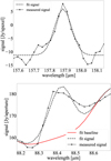 |
Fig. A.1 Spectra from location N158 indicated by the crosses in Fig. 1 averaged in apertures drawn around the location with a 15″ diameter. The measured spectra are shown by the connected black stars. The dashed black line shows the fit signal. For the [O III] spectra the fit baseline is additionally shown as a red line. Details of the line fit can be found in section 2.1.3. Top: [C II], Bottom: [O III]. |
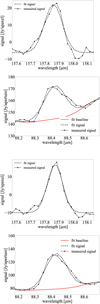 |
Fig. A.2 Same as figure A.1, but Top 2: N160; Bottom 2: N159. |
 |
Fig. A.3 Same as figure A.1, but with aperture diameters of 48″ for [O III]. From top to bottom: dif1, dif2, dif3, dif4. |
Appendix B Cross calibration with Herschel/PACS
This appendix reports the flux measurements performed in 20 different apertures observed by both SOFIA/FIFI-LS and Herschel/PACS.
PACS versus FIFI-LS cross-correlation
From a simulation.
From Herschel/SPIRE.
Using the rad. velocity from Table 1.
They compare [O III] to the 88 µm continuum, which they demonstrate exhibits a strong correlation with the 24 µm continuum.
All Tables
Observational parameters of SOFIA/FIFI-LS observations; the radial velocity was used to center the arrays spectrally and the beam size in parsecs was calculated based on a distance of 50 kpc; the integration time Tint is per FIFI-LS spatial pixel.
All Figures
|
Fig. 1 Intensity of the far-infrared fine-structure lines [C II]λ158 µm (left) and [O III]λ88 µm (right) in W m−2 sr−1, observed by SOFIA/FIFI-LS. The intensities are the result of spectral Gaussian fits and only those fits with a S/N ≥ 3 are shown. Pixels with lower S/N are displayed as 0 (in black). The white contours are from LTIR (300 and 600 Lso//pc2) shown in Fig. 3. The thin black contours shown in the [C II] map are 8 µm from Spitzer/IRAC (4 and 8 MJy/Sr). The red contours in the [O III] map are Spitzer/MIPS 24 µm continuum (5 and 150 MJy/sr). The [C II] map is shown in the native resolution with a beam FWHM of 15.3″. The [O III] data in the three bright star formation regions marked by dashed blue, green and red lines was smoothed to the same resolution (15.3″) to increase the S/N per beam. Outside of the regions the data was further re-binned to 24″ and fit within a 48″ beam to further increase the S/N in the diffuse regions. The seven gray crosses, in identical positions in the [C II] and [O III] maps, mark the positions of the spectra shown in Appendix A. |
| In the text | |
|
Fig. 2 RGB map of [C II] (r), [O III] (g) and 12CO(2−1) (b) from Tarantino et al. (in preparation) and Chen et al. (in preparation), with the map of the 12CO(2−1) outlined in white. Contours are shown for 12CO(2−1) line flux levels of 5 × 10¹¹ and 5 × 10¹⁰ Wm−2 sr−1. Regions for analyses in Sect. 4 are outlined, corresponding respectively to the SFRs, N159(green), N160(red), N158(blue), an extended, less active region in [O III] (yellow) and three CO-bright filaments (brown). They are also referred to in Fig. 3, and in the plots in Figs. 5 and 6. |
| In the text | |
|
Fig. 3 Map of TIR power in the molecular ridge. Regions for the analyses in Section 4 are outlined, corresponding, respectively, to the SFRs, N159 (green), N160 (dotted red), N158 (blue), an extended, less active region in [O III] (yellow), and three CO-bright filaments (dashed brown). They are also shown in Fig. 2, and used in the plots in Figs. 5, 4, and 6. |
| In the text | |
|
Fig. 4 L[C II]/LTIR versus LTIR in the molecular ridge in 12″× 12″ pixels. Yellow, blue, red, green, and brown colors refer to the regions outlined in Figs. 2 and 3. Gray points represent the pixels in the ridge outside of these regions. Data for 30 Doradus from Chevance et al. (2020) is added. The gray line represents the average minimum detectable [C II] line flux for S/N = 3. The large circles represent the ratio values for the whole ridge (cyan) and the three bright SFRs (N158: blue; N160: red; Nl59:green), relative to the mean LTIR. The areas with filled colors represent observations from: Orion A (Pabst et al. 2021); M51 (Pineda et al. 2018); N11B (Lebouteiller et al. 2012). |
| In the text | |
|
Fig. 5 Line ratio plots for the molecular ridge. Yellow, blue, red, green, and brown colors refer to the regions outlined in Figs. 2 and 3. Gray points represent the pixels in the ridge outside of these identified regions. Left: L[O III]/L[C II] versus LTIR in 12″ pixels for the three bright star formation regions and in 24″ pixels for the rest of the molecular ridge, where pixels with S/N below 5 are shown as upper limits. 30 Doradus data points from Chevance et al. (2020) have been added with 12″ binning. The horizontal lines show the mean L[O III]/L[O II] ratio for the regions. Right: L[O II]/LTIR versus L[CO]/LTIR in 12″ pixels. CO(1−0) was estimated from CO(2−1) assuming a ratio of CO(2−1)/CO(1−0) of 0.6 (e.g., den Brok et al. 2021; Maeda et al. 2022). The average ratio (no fit) of L[C II]/LCO(1−0) from the molecular ridge is indicated with the cyan line. The large circles represent the ratios based on the fluxes for the whole regions, in cyan for the whole molecular ridge and in matching colors for the three star formation regions. The area filled in red represents the data range for dwarf galaxies from Madden et al. (2020) using a LTIR to LFIR ratio of 0.6. |
| In the text | |
|
Fig. 6 [O III] emission versus 24 µm continuum emission (left) and versus Hα (right) in the three star formation regions in 12″ × 12″ pixels and at 48″ resolution (in 24″ × 24″ pixels) for the rest of molecular ridge map with a detection more than 5σ in both. Yellow, blue, red and green colors refer to the regions outlined in Figs. 2 and 3. Gray points represent the pixels in the ridge outside of these identified regions. For the diffuse regions shown in gray and yellow, fit results with a S/N below 5 are shown as upper limits. The black lines in the left plot show the fit linear relation and the 95% confidence interval from Lambert-Huyghe et al. (2022). |
| In the text | |
|
Fig. A.1 Spectra from location N158 indicated by the crosses in Fig. 1 averaged in apertures drawn around the location with a 15″ diameter. The measured spectra are shown by the connected black stars. The dashed black line shows the fit signal. For the [O III] spectra the fit baseline is additionally shown as a red line. Details of the line fit can be found in section 2.1.3. Top: [C II], Bottom: [O III]. |
| In the text | |
|
Fig. A.2 Same as figure A.1, but Top 2: N160; Bottom 2: N159. |
| In the text | |
|
Fig. A.3 Same as figure A.1, but with aperture diameters of 48″ for [O III]. From top to bottom: dif1, dif2, dif3, dif4. |
| In the text | |
Current usage metrics show cumulative count of Article Views (full-text article views including HTML views, PDF and ePub downloads, according to the available data) and Abstracts Views on Vision4Press platform.
Data correspond to usage on the plateform after 2015. The current usage metrics is available 48-96 hours after online publication and is updated daily on week days.
Initial download of the metrics may take a while.