| Issue |
A&A
Volume 702, October 2025
|
|
|---|---|---|
| Article Number | A3 | |
| Number of page(s) | 18 | |
| Section | Extragalactic astronomy | |
| DOI | https://doi.org/10.1051/0004-6361/202555935 | |
| Published online | 26 September 2025 | |
He II emitters at cosmic noon and beyond
Characterising the He II λ1640 emission with MUSE and JWST/NIRSpec
1
Instituto de Astrofísica de Andalucía (IAA-CSIC), Glorieta de la Astronomía s/n, E-18008 Granada, Spain
2
Observatório Nacional/MCTIC, R. Gen. José Cristino, 77, 20921-400 Rio de Janeiro, Brazil
3
Instituto de Astrofísica, Facultad de Física, Pontificia Universidad Católica de Chile, Av. Vicuña Mackenna, 4860 Santiago, Chile
4
Centro Astronómico Hispano en Andalucía, Observatorio de Calar Alto, Sierra de los Filabres, 04550 Gérgal, Spain
⋆ Corresponding author: This email address is being protected from spambots. You need JavaScript enabled to view it.
Received:
13
June
2025
Accepted:
1
August
2025
Abstract
The study of high-redshift galaxies provides critical insights into the early stages of cosmic evolution, particularly during what is known as cosmic noon, when star formation activity reached its peak. Within this context, the origin of the nebular He II emission remains an open question. For this work, we conducted a systematic multi-wavelength investigation of a sample of z ∼ 2–4 He II λ1640 Å emitters from the MUSE Hubble Ultra Deep Field surveys, utilising both MUSE and JWST/NIRSpec data and extending the sample presented by previous studies. We derived gas-phase metallicities and key physical properties, including electron densities, temperatures, and the production rates of hydrogen- and He+-ionising photons. Our results suggest that a combination of factors, such as stellar mass, initial mass function, stellar metallicity, and stellar multiplicity, likely contributes to the origin of the observed nebular He II emission. Specifically, for our galaxies with higher gas-phase metallicity (12 + log(O/H) ≳ 7.55), we find that models for binary population with Salpeter IMF (Mup = 100 M⊙) and stellar metallicity Z⋆ ≈ 10−3 (i.e. similar to that of the gas) can reproduce the observed He II ionising conditions. However, at lower metallicities, models for binary populations with a ‘top-heavy’ initial mass function (Mup = 300 M⊙) and Z⋆ much lower than that of the gas (10−4 < Z⋆ < 10−5) are required to fully account for the observed He II ionising photon production. These results reinforce that the He II ionisation keeps challenging current stellar populations, and the He II ionisation problem persists in the very low-metallicity regime.
Key words: ISM: abundances / galaxies: evolution / galaxies: high-redshift / galaxies: ISM / galaxies: star formation
© The Authors 2025
 Open Access article, published by EDP Sciences, under the terms of the Creative Commons Attribution License (https://creativecommons.org/licenses/by/4.0), which permits unrestricted use, distribution, and reproduction in any medium, provided the original work is properly cited.
This article is published in open access under the Subscribe to Open model. This email address is being protected from spambots. You need JavaScript enabled to view it. to support open access publication.
1. Introduction
The study of high-redshift galaxies offers critical insights into the early stages of cosmic evolution, particularly during what is called cosmic noon, a period around z ≈ 2–3 when star formation (SF) activity peaked (e.g. Lilly et al. 1995; Madau et al. 1996). Understanding the physical processes and stellar populations present during this epoch, and extending into the cosmic dawn at 6 ≲ z ≲ 10 when the first ionising sources emerged, is essential to fully understand the processes of cosmic reionisation and the subsequent evolution of the universe (e.g. Tumlinson & Shull 2000; Wise et al. 2012; Bromm 2013; Wise et al. 2014; Finkelstein et al. 2019). In this context, the budget of the double ionised helium (He++) is still a mystery. This ion produces recombination emission lines (He II); the most prominent features are the optical λ4686 Å and the ultraviolet (UV) λ1640 Å narrow lines. This implies the existence of very strong ionising radiation with photon energies higher than 54.4 eV (or λ ≤ 228 Å). In the far Universe, the presence of these nebular lines is observed to be more common in high-redshift galaxies than in local galaxies (e.g. Kehrig et al. 2011; Cassata et al. 2013; Kehrig et al. 2015, 2018), making the study of galaxies exhibiting nebular He II lines in their spectra (hereafter referred to as He II emitters) important in understanding the nature of the ionising sources, the physical conditions of the interstellar medium (ISM), and the stellar populations driving the early phases of cosmic evolution. In addition, the intensity of the nebular He II line is observed to be higher in lower metallicity galaxies (Guseva et al. 2000; Bromm 2013). In consequence, the presence of nebular He II lines in high-redshift galaxies is suggested as a tracer of Population III (PopIII; Schaerer 2002, 2008) stars, which are extremely hot and metal-poor (often considered essentially metal-free, Z ≈ 0) as they formed during the first million years of the universe from primordial hydrogen and helium. These stars would emit a significant hard UV ionising continuum, potentially making them major contributors to cosmic reionisation (e.g. Yoon et al. 2012; Cassata et al. 2013; Nakajima & Maiolino 2022). Although a prominent PopIII ionising continuum meets the conditions required to produce strong He II and Lyα lines in high-redshift star-forming galaxies as observed at z > 6 with HST (e.g. Cai et al. 2011) and JWST (e.g. Topping et al. 2024; Venditti et al. 2024; Mondal et al. 2025), this becomes a problem at lower redshifts, where the presence of PopIII stars becomes increasingly unlikely.
Wolf–Rayet (WR) stars were proposed as a candidate to solve this problem, (Garnett et al. 1991; Schaerer 1996). WR stars are massive evolved stars in a late evolutionary stage, where core helium burning occurs and the hydrogen envelope is stripped away (Allen et al. 1976; Izotov & Thuan 2004; Roy et al. 2020, 2025). In this phase, some early-type WR stars are characterised by intense mass loss driven by dense and powerful stellar winds, while the stripped stellar surface reaches extremely high temperatures (T ∼ 100 kK) capable of doubly ionising the helium. WR winds can explain the origin of the nebular He II in high-metallicity galaxies (Shirazi & Brinchmann 2012; Roy et al. 2025). In particular, systematic studies using integral field spectrographs (IFS) such as VIMOS (Le Fèvre et al. 2003; Cassata et al. 2013) and MUSE (Bacon et al. 2010; Nanayakkara et al. 2019), as well as observations in individual galaxies such as NGC1569 with MEGARA (Mayya et al. 2020) or the Cartwheel Galaxy with MUSE (Mayya et al. 2023), have found that nebular He II emission is most likely powered by WR stars. However, the problem persists in HeII-emitting metal-deficient star-forming galaxies, where WR features are not prominent (e.g. Izotov & Thuan 2004; Kehrig et al. 2018; Nanayakkara et al. 2019; Roy et al. 2025). WR stars are not expected to be seen in the spectra of extremely metal-poor galaxies (Z ∼ 0.03 Z⊙) such as SBS 0335-052E (Izotov et al. 1999) and IZw18 (Thuan et al. 2004). In these cases and in similar extremely metal-poor galaxies (Pérez-Montero et al. 2020), the ionising power of the WR populations has been found insufficient to supply the UV radiation required to fully ionise He+, leaving this scenario still open to debate. On the other hand, interacting binary stellar populations composed of young massive stars have also been shown to reproduce similar ionising conditions, particularly in metal-poor environments (Z ∼ 0.03 Z⊙) with a top-heavy initial mass function (IMF). These conditions favour the formation of stars with higher surface temperatures, resulting in a harder ionising spectrum and a greater production of photons with energies exceeding 54.4 eV (e.g. Eldridge & Stanway 2012; Eldridge et al. 2017; Götberg et al. 2017; Smith et al. 2018; Götberg et al. 2019, 2023). According to binary stellar evolution models such as BPASS (Eldridge et al. 2017; Xiao et al. 2018), the predicted ionising flux from systems that include metal-poor binary interactions, stellar rotation, and a top-heavy IMF can account for the overall He II photon budget (e.g. Kehrig et al. 2018; Nanayakkara et al. 2019; Hawcroft et al. 2025). Nevertheless, in extremely metal-poor galaxies, these models cannot fully account for the He II photon production when the stellar Z is the same as that of the gas, even when including contributions from X-ray photons (e.g. Senchyna et al. 2020; Kehrig et al. 2021), shocks (Götberg et al. 2023) or gas-stripping processes (e.g. Götberg et al. 2017, 2023). This limitation necessitates invoking nearly metal-free stars, suggesting a decoupling between stellar and gas-phase metallicities (e.g. Kehrig et al. 2018; Eldridge & Stanway 2022).
In general, the origin of the nebular He II emission is often attributed to WR stars or metal-poor binary systems with a top-heavy IMF in high-metallicity and metal-poor galaxies (up to 12 + log(O/H) ≈ 8; Kehrig et al. 2018; Nanayakkara et al. 2019; Pérez-Montero et al. 2020). However, an apparent anti-correlation between He II photon production and gas-phase metallicity has been observed, which remains largely unexplained (e.g. Shirazi & Brinchmann 2012; Schaerer et al. 2019; Pérez-Montero et al. 2020; Roy et al. 2025). Commonly invoked ionising sources, such as those mentioned, appear insufficient to account for the observed He II photon production as the gas-phase metallicity of the emitters decreases, indicating that additional ionising mechanisms may be required, especially in extremely metal-poor galaxies (7.2 ≲ 12 + log(O/H) ≲ 7.7; Kehrig et al. 2015, 2016, 2018). This is one of the primary reasons why PopIII-like stars are often invoked in such scenarios, as their extremely hot metal-free nature enables them to produce the hard ionising continuum required to explain the observed He II emission in the most metal-poor galaxies (e.g. Schaerer 2008, 2002; Cassata et al. 2013; Nanayakkara et al. 2019; Nakajima & Maiolino 2022). However, most studies that explore the He II ionisation budget in detail tend to focus on individual galaxies–such as Cartwheel or SBS 0335-052E with MUSE (e.g. Kehrig et al. 2016, 2018; Mayya et al. 2020, 2023)–without testing whether the observed anti-correlation between He II emission and gas-phase metallicity is also present in other galaxies. On the other hand, larger systematic studies using integral field units (IFUs), such as Cassata et al. (2013) with VIMOS and Nanayakkara et al. (2019) with MUSE, often do not fully exploit the rich two-dimensional spatial and spectral information that these instruments can provide.
The aim of this study was to carry out a systematic multi-wavelength investigation of the He II ionisation budget by analysing a sample of He II-emitting star-forming galaxies observed with the MUSE instrument, extending the dataset originally presented by Nanayakkara et al. (2019). We made use of all available emission lines with a sufficiently high and reliable signal-to-noise ratio (S/N) in the MUSE Hubble Ultra Deep Field surveys (Bacon et al. 2017, 2023) and complemented the MUSE data with observations from the James Webb Space Telescope’s Near-Infrared Spectrograph (JWST/NIRSpec). This combined dataset allowed us to derive the gas-phase abundances of our He II emitters and to perform a series of diagnostic analyses involving the He II λ1640 line in conjunction with other key UV features, such as [O III] λ1661,1666, [C III] λ1907,1909, and C IV λλ1548,1551, in order to constrain the origin of the He II ionisation.
The structure of this paper is as follows. Section 2 presents the MUSE and JWST sample, outlining the selection criteria and characterisation of the galaxies. In Section 3 we derive the gas-phase metallicities and determine key physical properties, including the electron density and the production rates of hydrogen- and He+-ionising photons. Section 4 compares our results with the photoionisation models of Gutkin et al. (2016) and the BPASS binary stellar population models in order to constrain the possible origins of the He II emission. Additionally, we discuss potential discrepancies between metallicity estimates based on UV calibrators and those obtained via direct methods using electron temperature measurements from JWST data. We also examine the impact of dust reddening across different wavelengths.
We adopt the standard ΛCDM cosmology with H0 = 70 km/s/Mpc, ΩΛ = 0.7, and ΩM = 0.3.
2. Sample characterisation
2.1. MUSE sample
The physical characterisation of He II emitters requires medium to high spectral resolution (R ≳ 1000) in order to discriminate the nebular He II line, along with broad spectral coverage to discern key UV features such as the [O III] λ1661,6 and [C III] λ1907,9, as well as Lyα emission. The Multi-Unit Spectrographic Explorer (MUSE; Bacon et al. 2010) IFS at the ESO-VLT 8.2m telescope offers a rest-frame spectral range of 4650 − 9300 Å, with a resolution varying from 1750 at 4650 Å to 3750 at 9300 Å, and a spectral sampling of 1.25 Å. It provides a field of view (FoV) of 1 arcmin2 with a spatial sampling of 0.2 × 0.2 arcsec. These characteristics enable the detection of the He II line in galaxies from the cosmic noon to earlier epochs (1.9 < z < 4.7).
Our sample was selected from the MUSE Hubble Ultra Deep Field surveys (MHUDF; Bacon et al. 2017), comprising three MUSE fields: the MUSE eXtremly Deep Field (MXDF, 141-h depth), the Ultra Deep Field survey (UDF-10, 1 arcmin2 31-h depth field), and the 3×3 arcmin mosaic of nine MUSE fields with 10-h depth (MOSAIC). The MHUDF data release includes 2221 different spectroscopic sources detected in those surveys (Bacon et al. 2023), all of them published in The Advanced MUSE Data products (AMUSED) web interface1. The available data products include datacubes that have already been reduced using a scheme to remove systematics and a self-calibration process to mask instrumental artefacts (see Bacon et al. 2017 for more details regarding the data reduction). Additionally, the Zurich Atmospheric Purge (ZAP) software (Soto et al. 2016) was applied to remove sky residuals and improve the overall datacube quality. The database includes a reference observed spectrum for each source, along with the corresponding continuum model and line fittings. The reference spectrum represents the observed integrated spectrum of the source, where the detected sources within the datacube and subsequent extraction were performed using the ORIGIN2 software (Mary et al. 2020), which is optimised for detecting faint emission sources in MUSE datacubes. Figure 1 presents an example of a source detected in this work and included in the AMUSED database. The left panel displays a white-light continuum image extracted directly from the MUSE datacube, while the central panel shows the segmentation map generated by the ORIGIN software, from which the reference spectrum was extracted, and the right panel shows the corresponding HST F606W filter image. The lower panel presents the spectrum extracted using the ORIGIN segmentation map (in blue), along with the continuum model and line fitting (in red), measured using the PYPLATEFIT tool. This tool was specifically developed to analyse the line features present in this dataset (Bacon et al. 2023), measuring the fluxes, errors, S/N, and FWHM for ∼65 lines that are included in the dataset. Additionally, the spectral energy distribution (SED), stellar mass, and star formation rate (SFR) for each detection, computed with PROSPECTOR (Johnson et al. 2021) using Hubble Space Telescope (HST) photometry, are also provided.
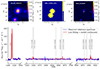 |
Fig. 1. Example of a detected source from MHUDF, representing the galaxy with ID 106 in the MXDF. Upper panels: MUSE white-light image (left), ORIGIN segmentation map of the source (centre), and HST F606W filter image (right). Lower pannel: Observed reference spectrum of the source extracted with ORIGIN (blue) and its respective continuum + emission line fit (red). |
This dataset has already been used in a wide variety of works such as those involving the Lyα luminosity function (Drake et al. 2017), the MgII emission (Feltre et al. 2018), or extreme emission line galaxies (del Moral-Castro et al. 2024). From this dataset we selected only sources with a S/N in the He II line greater than 3. Only 25 out of the 2221 sources meet this criterion, two of which are confirmed active galactic nuclei (AGNs; ID:1051 and ID:1056; Nanayakkara et al. 2019), which present broad He II, [C III], and C IV features. We identified a greater number of He II emitters in the MHUDF compared to previous studies (e.g. Nanayakkara et al. 2019); five of these sources are present in the Nanayakkara et al. (2019) dataset (without taking into account the two AGNs; see for more details). In addition, 12 of them also present a prominent Lyα emission line. We note that we do not know whether the rest of the galaxies present Lyα emission since the 1216 Å wavelength is outside the spectral range at that redshift;3 however, it is important to note that all the galaxies in this sample that show He II emission also show Lyα emission when the λ = 1216 Å is in the observed rest-frame spectrum, when, in general, not necessary a galaxy with He II emission present Lyα (Cassata et al. 2013). Figure A.1 shows the He II emission detected in the 25 sources; the observed and fitted spectra (blue and red, respectively) are the reference and the continuum + fit spectrum as in Figure 1. Additionally, the figure shows the He II S/N and Lyα S/N for galaxies where Lyα is detected. All galaxies present a clearly visible and prominent He II line; furthermore, the Lyα emission is also prominent (except for ID:103), with S/N > 100 in some cases. A detailed spatially resolved analysis of Lyα profiles will be done in a forthcoming paper as half of the Lyα emitters in this sample exhibit a double-peaked profile, and, in general, all are partially absorbed.
The main characteristics of the sample are listed in Table B1 (all tables can be found in Appendix B). Figure 2 shows the classical star formation main sequence (SFMS) for our sample (excluding the two AGNs), covering a stellar mass (M⋆) distribution in the range  with a median of
 , as well as a SFR distribution of
 with a median value of
 . These galaxies span 1.907 < z < 4.41, with a median z = 2.974, thus one-half of the sample lies beyond the cosmic noon (z > 3). The z = 3 theoretical SFMS derived by Boogaard et al. (2018) is also shown, exhibiting a small offset with the data. This offset, also reported by Bacon et al. (2023) for the entire HMUDF sample, is likely due to differences in the SFR calculation methods used by Boogaard et al. (2018) and Bacon et al. (2023) (see the latter for more details).
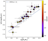 |
Fig. 2. Stellar mass vs. star formation rate for the sample, derived from the SED reported in the AMUSED database (Bacon et al. 2023), colour-coded by redshift and excluding the two AGNs. The z = 3 SFMS, as derived by Boogaard et al. (2018), is represented by a dashed blue line. The sample shows a slight offset relative to the z = 3 SFMS, but follows the expected linear trend. |
A summary of the observed fluxes, errors, and FWHMs of all lines detected in the sample is given in Table B2 (the full table is available online). The table includes all emission and absorption lines detected in the galaxies; there are a total of 54 lines ranging between the Lyα emission at 1216 Å and the MgI absorption line at 2853 Å. Only lines presenting a S/N greater than 3 are considerer in the analysis; the rest are excluded. Consequently, undetected lines (outside the wavelength range or having a low S/N) are represented as blank spaces in the table.
We derived the dust attenuation AV from the continuum UV slope β, parametrising the continuum as a power law (Calzetti et al. 1994): fλ ∝ λβ, where fλ is the observed flux at a wavelength λ. The emission and absorption UV features within the fitting range (1300–1900 Å) are masked to prevent them from altering the continuum shape; these features are listed in Table 2 of Calzetti et al. (1994). The β slope can be related with the total extinction at λ = 1600 Å as A1600 = 4.43 + 1.99β (Meurer et al. 1999), and thus the AV derived from β is
 (1)
(1)
with k1600 = 9.97 derived from Calzetti et al. (2000) extinction curve at λ = 1600 Å and RV = 4.05 the total V attenuation (Calzetti et al. 2000). Four of the galaxies present an insufficient continuum S/N to perform a reliable power-law fitting, giving a negative β slope. For those cases (shown as blank spaces in the AV column of Table B1) we assume that AV = 0; for the rest, we correct all the fluxes using the Calzetti et al. (2000) extinction curve:  .
.
Once the fluxes are corrected for extinction, we compute the UV magnitude, defined as the absolute magnitude at the 1500 Å band (M1500), i.e. the absolute AB magnitude derived from a simulated filter centred at λ = 1500 ± 100 Å. We obtain M1500 by computing a running median, averaging the convolution of the corrected flux between 1400 and 1600 Å with a window of size 20 Å. M1500 uncertainties are obtained as the standard deviation of 10 000 Monte Carlo runs.
The magnitudes obtained are distributed between −17 ≳ M1500 ≳ −22 with a median of ∼ − 18, which is comparable with the UV magnitudes of the He II emitters reported by other authors (e.g. Nanayakkara et al. 2019). Both M1500 and AV values are included in Table B1, along with the derived rest-frame He II and Lyα equivalent widths (EWs). These EWs were calculated using the observed and continuum-fitted spectra available in the AMUSED database, following the definition: EW = ∫(1 − Fo/Fc)dλ, where Fo and Fc represent the observed flux and the continuum-fitted flux, respectively. The EW is computed by centring the integral on the target line (1216 Å for Lyα and 1640 Å for He II) within a 20 Å window.
2.2. JWST-NIRSpec optical sample
In addition to the MUSE UV rest frame data of the sample data, we included a complementary rest-frame optical dataset for the sample as having simultaneous optical and UV data enables a more comprehensive analysis of the physical and chemical properties of these galaxies. The spectroscopic data from the Near-Infrared Spectrograph on the James Webb Space Telescope (NIRSpec-JWST) gives a wide range of emission and absorption features in the near-infrared (0.6–5.3 μm). At the redshift range of our galaxies (1.9 < z < 4.4), this spectral coverage corresponds to the optical regime, making NIRSpec spectra the ideal dataset for the mentioned task. NIRSpec gives spectra measured with different configurations, including a prism and several filter–grating combinations. The prism covers the entire NIRSpec spectral range, but at low resolution (R ∼ 100), causes a full blending of important emission lines, such as the Hα + [N II] λλ6548, 84 doublet or the [O III] λλ4959, 5007 doublet. In consequence, we used spectra taken with the grating–filter combinations G140M-F070PL, G235M-F170LP, and G395-F290LP, which provide medium resolution (R ∼ 1000) and a coverage of 0.70–1.27 μm, 1.66–3.07 μm, and 2.87–5.10 μm, respectively.
In order to include a homogeneously reduced and comprehensive NIRSpec dataset, we conducted an extensive search in the DAWN JWST Archive (DJA), a public repository of JWST galactic photometric and spectroscopic data, reduced using the GRIZLI4 and MSAEXP pipelines5 (Valentino et al. 2023; Heintz et al. 2024; de Graaff et al. 2025). We found in the DJA that only 5 of the 25 galaxies in our sample have reduced spectroscopic data for at least one of the mentioned filter–grating combinations, all of which were included in the JWST Advanced Deep Extragalactic Survey (JADES; D’Eugenio et al. 2025). Figure 3 presents an example of a 2D and a 1D NIRSpec spectrum for the galaxy with ID:50, obtained using the G235M/F170LP grating–filter combination. The figure also includes a NIRCam RGB cutout of the galaxy, created using the F115W, F277W, and F444W filters (top), along with a NIRCam F444W cutout displaying the NIRSpec slit location, marked by a magenta rectangle6. This galaxy exhibits the largest number of detected lines, ranging from Lyα at 1216 Å to Paγ at 10 938 Å, offering an extensive dataset that spans from the UV to the near-IR.
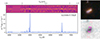 |
Fig. 3. Reduced 2D and 1D NIRSpec spectrum of the galaxy with ID:50 at z = 3.325, obtained using the G235M/F170LP grating–filter combination. The right panels display a NIRCam RGB cutout of the galaxy, constructed using the F115W, F277W, and F444W filters (top), and a F444W cutout with the NIRSpec slit location overplotted in magenta (bottom). Both NIRCam cutouts were obtained from the GRIZLI public database. |
We measured all the emission lines available within the spectral range of every galaxy, modelling the continuum as a power-law function, and using the Python MPFIT7 module to fit the lines. This module enables multi-peak Gaussian fitting for systems of multiplet lines, such as the Hα + [N II] λλ6548, 84 doublet or the [O III] λλ4959, 5007 doublet (see González-Díaz et al. 2024 for more details). Table B3 shows the flux, error, and FWHM of the emission lines measured in the NIRSpec sample. As for the UV lines in Section 2.1, we only considered those lines with a S/N greater than 3.
This compilation of 1D MUSE and JWST data provided a diverse and heterogeneous sample, allowing the physical characterisation of He II emitters and the measurement of chemical abundances, due to the large number of available emission lines. Furthermore, the complementary JWST/NIRSpec data allowed a more in-depth study of metallicity, electron temperature, and density. In addition, the MUSE 2D data available in the AMUSED database enabled the study of He II extended emission. The 2D characterisation, along with the analysis of Lyα profiles, will be approached in a future paper.
3. He II emitters physical and chemical properties
3.1. Metallicity determination
Nebular emission-line models predict that gas-phase metallicity and the hardness of the ionising SEDs are sensitive to UV stellar absorption, where nebular lines make a significant contribution in both local and high-redshift galaxies and, consequently, UV fluxes correlate with gas-phase metallicity (Byler et al. 2017, 2018). In particular, since [C III] λ1907 is one of the brightest UV lines, along with [O III] λ1661,6 Å, these lines, together with He II 1640 Å, have proven to be promising UV metallicity calibrators (Feltre et al. 2016; Jaskot & Ravindranath 2016) yielding results similar to those obtained from direct optical determinations (Byler et al. 2020; Iani et al. 2023).
We used the optimal 2D polynomial fitted to the model grid surface obtained in Byler et al. (2020), which relates the gas-phase metallicity with the He2-O3C3 diagnosis as
 (2)
(2)
where x is log10([O III] λ1666/[C III] λ1906,9) and y is log10(He II λ1640/[C III] λ1906,9).
Out of the 25 galaxies, we calculated the metallicity for 18, as the remaining galaxies have a signal-to-noise ratio (S/N) lower than 3 in at least one of the involved emission lines. Figure 4 presents the He2-O3C3 diagnostic diagram for these 18 galaxies. Three red lines are plotted, representing the polynomial from Equation (2) at fixed values of 12 + log(O/H) (7.3, 7.5, and 7.7, respectively). The metallicity values for the galaxies can be found in Table B4, in the range between 7.3 and 7.7 and with uncertainties of ∼±0.15, which places them within the low-Z regime; only two galaxies from our sample show metallicities (≈7.3) slightly above those (12 + log(O/H) ≈ 7.2–7.3) of the well-known extremely metal-deficient He II emitters IZw18 and SBS0335-052E (e.g. Izotov et al. 1999; Thuan et al. 2004; Kehrig et al. 2016, 2018), which show relatively low M⋆: 106.63 M⊙ for IZw18 (Zhou et al. 2021) and 107.43 M⊙ for SBS 0335-052E (Hunt et al. 2014). In our galaxy sample, the stellar masses range from 107.98 M⊙ to 1011.63 M⊙, with metallicity appearing to increase in more massive galaxies (see Figure 4).
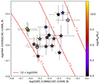 |
Fig. 4. He2-O3C3 diagnosis diagram. The red lines represent the polynomial from equation (2) at 12 + log10(O/H) = 7.3, 7.5, and 7.7 respectively. The colours indicate stellar mass, while the open points correspond to galaxies without SED information, and consequently no measured M⋆. Only 18 points are shown as the rest present a S/N lower than 3 in at least one of the involved emission lines. All galaxies fall within a metal-poor regime; three of them approach the extremely metal-poor regime (12 + log(O/H) ≈ 7.3), showing a trend with M⋆. |
The C/O and N/O ratios were determined using the empirical relationship with metallicity derived by Dopita et al. (2013) and later modified by Byler et al. (2020) to better match observations in the low-metallicity regime (12 + log(O/H) < 8). The relationships are defined as
 (3)
(3)
 (4)
(4)
with Z = 12 + log(O/H).
Carbon is often referred to as a pseudosecondary element since the triple-α process is not directly dependent on metallicity. Instead, variations in the C/O ratio are typically linked to other metallicity-dependent processes, such as stellar winds or supernova explosions, rather than nucleosynthesis (Berg et al. 2016; Byler et al. 2020). On the other hand, as the nitrogen forms as a secondary nucleosynthesis product at high metallicities, in our case it is expected to be constant (Dopita et al. 2013; Berg et al. 2016; Byler et al. 2020). Table B4 shows the C/O and N/O values for our sample with typical statistical errors of ±0.14 dex (Byler et al. 2020). The log(C/O) ratio ranges from −0.85 to −0.65, corresponding to −0.6 < [C/O] < −0.48. Other rest-frame UV calibrations for deriving C/O abundances exist, such as the semi-empirical method presented by Pérez-Montero & Amorín (2017), which used the [C III], C IV, and [O III] doublets. They found that for galaxies at z > 2, the log(C/O) abundance ranges from −0.8 to −0.5 for  , which is in very good agreement with our results. In addition to C/O, the log(N/O) abundance remains constant at ≈ − 1.5 ([N/O] = −0.42; Asplund et al. 2021), reinforcing the fact that all our He II emitters belong to a low-metallicity regime.
3.2. Electron density
The electron density (ne) is defined as the number of free electrons per unit volume. By selecting two emission lines from the same ion that originate from nearly identical excitation energy levels, the relative excitation rate becomes primarily dependent on the collision strength (Osterbrock & Ferland 2006). In such cases, if the collisional de-excitation rates of the two levels are different, the intensity ratio of these lines will depend mostly on the electron density. Traditionally, the optical [S II] λ6716/λ6731 ratio has been used to estimate ne. However, in the UV regime, the [C III] λ1907/λ1909 ratio exhibits similar characteristics, making it a suitable diagnostic for determining the electron density in this dataset (Keenan et al. 1992; Osterbrock & Ferland 2006; Proxauf et al. 2014). We used PYNEB, as described in Section 3.1, assuming an electron temperature of Te = 104 K. The [C III] λ1907/λ1909 ratio is employed to estimate the electron density for those galaxies in which both [C III] lines are detected with a S/N greater than 3. For galaxies with ID 50, 22, and 1141, we instead used the optical [S II] ratio from NIRSpec observations as the S/N of the [S II] lines is higher than that of the [C III] doublet in these cases. The uncertainties associated with every value are obtained as the standard deviation of 10 000 Monte Carlo runs. Table B4 summarises the values obtained for each galaxy. We find that the galaxies present low to intermediate ne regimes, between 102–103 cm−3, with only two cases with ne ≈ 104 cm−3. However, it is important to note that the uncertainties associated with the derived values are significant (up to 50%) due to the [C III] lines, which are intrinsically faint and therefore noisy.
3.3. Ionising photon production
The presence of the nebular He II 1640 Å line in at high redshift indicates the existence of hard ionising radiation, requiring photons with energies hν > 54.4 eV to ionise the He+ ion, which is characteristic of ongoing extreme star formation activity in very low-metallicity regimes (Kehrig et al. 2011; Kehrig et al. 2015, 2018; Cassata et al. 2013).
These photons produce an ionising flux that is related to the He II 1640 Å luminosity as follows (Osterbrock & Ferland 2006):
![Mathematical equation: $$ \begin{aligned} Q_{\rm He\,{\footnotesize II}} = \frac{L_{1640}}{j_{1640}\alpha _{\rm B}(\mathrm{He\,{\footnotesize II}}_{1640},T)} \quad [\mathrm {phot}/\mathrm s]. \end{aligned} $$](/articles/aa/full_html/2025/10/aa55935-25/aa55935-25-eq14.gif) (5)
(5)
Here L1640 is the He II 1640 Å luminosity, reddening corrected using the AV derived from equation (1); j1640 is the He II 1640 Å emissivity; and  is the recombination coefficient for the He II 1640 Å at a given temperature.
Analogously, we can also calculate the hydrogen photon production rate using the Hα line as
![Mathematical equation: $$ \begin{aligned} Q_{\rm H\alpha } = \frac{ L_{\rm H\alpha }}{j_{\rm H\alpha }\alpha _{\rm B}(\mathrm{H\alpha },T)} \quad [\mathrm {phot}/\mathrm s], \end{aligned} $$](/articles/aa/full_html/2025/10/aa55935-25/aa55935-25-eq16.gif) (6)
(6)
where LHα is the Hα 6563 Å luminosity, jHα is the Hα emissivity, and αB(Hα, T) is the recombination coefficient for the Hα line at a given temperature. We computed both QHeII and QHα using the Python module PYNEB (Luridiana et al. 2015) assuming case B recombination, T = 104 K, and an electron density ne = 100 cm−39. Since the Hα line is not included in the sample, we estimated LHα using the SFR derived from the SED (Table B1) and applying the SFR-LHα relation (Kennicutt et al. 1994; Madau et al. 1998; Kewley & Dopita 2002): SFR .
.
Figure 5 shows the relation between He++ versus H+ ionising photon production. Given that the ionisation potential of He+ (54.4 eV) is significantly higher than that of H0 (13.6 eV), it is expected that QHα ≥ QHeII; if the incident SED is hard enough to doubly ionise helium, it is also sufficient to ionise hydrogen. In addition, the trend in Figure 5 appears to be exponential, with the minimum value of QHα (1052.94) reached at the minimum value of QHeII (1052.26), and the maximum value of QHα (1055.71) reached at the maximum value of QHeII (1054.33; individual values can be found in Table ). Furthermore, both QHeII and QHα appear to correlate with the stellar mass (see Figs. 5 and 6). On the one hand, a correlation between M⋆ and QHα is expected, as QHα is proportional to the SFR, and the SFR and M⋆ follow a linear trend in the SFMS (Figure 2). On the other hand, Fig. 6 shows that QHeII values seem to increase with the absolute UV magnitude (M1500) and with the total stellar mass of our galaxy sample of nebular He II emitters. These trends indicate that hot massive stars might be the main cause of the He II ionisation in our sample since such stars are expected to dominate the far-UV stellar continuum at 1500 Å and the stellar mass in metal-poor star-forming galaxies (e.g. Guseva et al. 2000; Shirazi & Brinchmann 2012; Kehrig et al. 2015; Szécsi et al. 2015; Kehrig et al. 2016, 2018; Senchyna et al. 2020; Berg et al. 2021). This is also expected since brighter galaxies have more star formation, and thus there can be more stars that can contribute to the ionising photon production.
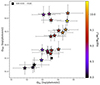 |
Fig. 5. He++ vs. H+ ionising photon production, derived from Equations (5) and (6). The colours indicate the stellar mass of each galaxy. The black square represents measurements for the extremely metal-poor star-forming galaxy SBS 0335-052E taken from Kehrig et al. (2018). |
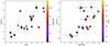 |
Fig. 6. QHeII in units of log(photons/s) as a function of UV magnitude (left panel) and of stellar mass (right panel). The colours indicate the stellar mass of each galaxy. The relationship between the two ionising photon production rates appears to be exponential, with both quantities increasing as a function of stellar mass. |
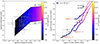 |
Fig. 7. Left: [C III] λ1907/He II – [O III] λ1666/He II diagnosis. The Gutkin et al. (2016) models plotted correspond to a pure photoionisation scenario due to massive stars with log(Us) = − 1, ξd = 0.1, mup = 300 M⊙, and |

4. Discussion
4.1. UV diagnosis diagrams
The characterisation of star formation and ISM conditions in star-forming galaxies and AGNs requires a comprehensive interpretation of optical and/or UV emission lines. The computation of stellar population synthesis and photoionisation codes leads to the generation of various nebular emission models, which can be used to interpret the observed emission line fluxes. Furthermore, the He II λ1640 line is commonly used as a standard reference in UV diagnostics, which is analogous to Hβ in optical diagnostics, due to its strong dependence on both the metallicity and the ionisation parameter (Feltre et al. 2016). In particular, Gutkin et al. (2016) present a set of UV models based on stellar population synthesis models (Bruzual & Charlot 2003) and CLOUDY photoionisation models (Ferland et al. 2013). These models are suitable for studying the chemical evolution and ISM properties of galaxies at high redshift (2 ≲ z ≲ 9) based on UV emission features (e.g. Gutkin et al. 2016; Feltre et al. 2016; Stark et al. 2017; Nanayakkara et al. 2019; Bunker et al. 2023; Atek et al. 2024), and are parametrised using six values, which are more sensitive to UV lines than optical lines: the total ISM metallicity (ZISM), the hydrogen gas density (nH), the zero-age ionisation parameter at the Strömgren radius (Us), the dust-to-metal ratio (ξd), the upper mass cut-off of the initial mass function (mup), and the C/O ratio.
In Figure 7 (left) we show the [C III] λ1907/He II versus [O III] λ1666/He II diagnosis. The models plotted correspond to a pure photoionisation scenario due to massive stars, as pure AGN ionisation would produce [C III]/He II ratios lower than 1 (Feltre et al. 2016; Gutkin et al. 2016). These models, which best fit the data, correspond to the highest ionisation parameter in the set, with log(Us) = −1, a low dust-to-metal ratio (ξd = 0.1), and a top-heavy IMF with mup = 300 M⊙. The free parameters are the ISM metallicity (ZISM), expressed in terms of 12 + log(O/H), and the C/O abundance (normalised to (C/O)⊙ = 0.55; Asplund et al. 2021), represented in Figure 7 as an area with a width corresponding to ZISM and a height corresponding to C/O. All points fall within this area, with values of 12 + log(O/H)model < 7.7, which are similar to the values found in Section 3.1. The C/O values range between 0.14(C/O)⊙ and 0.27(C/O)⊙, corresponding to −0.85 < [C/O] < −0.4, generally falling below the measured values shown in Section 3.1 (−0.6 < [C/O] < −0.4). These variations in the C/O ratios when using UV lines are well documented in the literature and can fluctuate by more than 0.6 dex at low metallicities (Berg et al. 2016, 2019; Byler et al. 2020). This is primarily due to the strong dependence of C/O on the star formation history (SFH) and supernova feedback, and thus the [C III] and [O III] lines alone are insufficient to accurately determine the gas-phase oxygen abundance (Berg et al. 2019; Byler et al. 2020).
In addition, the diagnostic diagrams that best distinguish between star formation-driven photoionisation, AGN activity, and shocks are those involving the UV lines C IV λλ1548, 51, [C III] λ1907, and He II λ1640, as AGNs and shocks produce markedly different line ratios in the UV compared to their optical counterparts (e.g. Villar-Martin et al. 1997; Allen et al. 1998; Groves et al. 2004; Allen et al. 2008; Feltre et al. 2016). In addition, the ratios involving the lines mentioned above have been found to be sensitive to metallicity, and the C IV λλ1548, 51/[C III] λ1907 ratio also depends on the ionisation parameter (Nagao et al. 2006; Feltre et al. 2016). In Figure 7 (right) we examine the C IV λλ1548, 51/[C III] λ1907 versus C IV λλ1548, 51/He II diagnosis using the Gutkin et al. 2016 models as in Figure 7 (left).
The figure shows the mentioned line ratios for all our galaxies where the C IV lines are detected, including the two AGNs (ID:1051 and ID:1056), exhibiting a linear trend between the two ratios as the C IV λλ1548, 51 flux increases. This behaviour correspond with a photoionisation scenario driven by star formation in most galaxies. However, the trend breaks for the two AGNs, which show significantly higher C IV λλ1548, 51 emission relative to the other lines, which is an expected signature of AGN activity (Gutkin et al. 2016; Feltre et al. 2016). The coloured lines represent models for pure star-forming photoionisation with the same gas density of nH = 102 cm−3 and three different ionisation parameters (from log(Us) = −3 to −1). The rainbow-coded colours indicate the metallicity, ranging from 12 + log(O/H) = 7 to 8.75. An increase in ISM metallicity is also expected to lead to a higher abundance of cooling agents, resulting in an increased ratio of metal lines to He II emission (Gutkin et al. 2016), and thus the increment in the C IV/He II ratio of Figure 7 (right) translates into a metallicity gradient. For similar metallicity values, C IV/[C III] increases with the ionisation parameter. For a fixed Us, the models show that the increase in the C IV λλ1548, 51 emission relative to the collisionally excited [C III] line in our galaxies can be attributed to an increase in metallicity, which is compatible with our measured values of 12 + log(O/H) < 7.7. Since Us is proportional to the H-ionising photon rate (QH) and to the gas density nH, this parameter provides insight into the hardness of the ionising spectrum. A high Us can result from AGN activity, which tends to increase the gas density and ionising output, or from elevated ionising photon production (Feltre et al. 2016). As discussed in Section 3.3, QH can be higher than 1054 photons/s in star-forming galaxies, particularly in the most massive He II emitters.
4.2. Direct vs indirect abundance determination
The use of UV lines to estimate chemical abundances in high-redshift star-forming galaxies has been extensively discussed by several authors (e.g. Villar-Martín et al. 2004; Yuan & Kewley 2009; Erb et al. 2010; Christensen et al. 2012; James et al. 2014; Bayliss et al. 2014; Steidel et al. 2016; Kojima et al. 2017; Nicholls et al. 2020). All these studies found that using the UV lines of the O++ ion yields Te values similar to those obtained from optical lines, showing the importance of using UV lines to characterise physical conditions in high-redshift galaxies (see Nicholls et al. 2020 for more details). In particular, UV [C III] and [O III] lines are optimal for this estimation since the emissivity of [O III] λ1666 Å and the strength of the [C III] λ1909 Å line are sensitive to Te and the oxygen gas abundance rather than the absolute carbon abundance. Thus, the combination of [C III] and [O III] emission lines serves as a tracer of the gas-phase oxygen abundance (Jaskot & Ravindranath 2016; Byler et al. 2018, 2020).
Galaxy 50 is the one with the broadest wavelength coverage when combining MUSE and NIRSpec data, allowing a direct estimation of Te using the [O III] UV doublet 1660,66 and the optical [O III] 5007 Å line. Nicholls et al. (2020) presents a formula for obtaining Te by combining optical and UV O++ ion lines, obtained by fitting several line ratios obtained from MAPPINGS V5.1 photoionisation models, using extensive collisional and radiative excitation/de-excitation data, as well as collisional cross-sections from Lennon & Burke (1994). This fitting assumes a low-density limit and a Te range between 5000 and 32 000 K. The results obtained by Nicholls et al. (2020) from this fitting are consistent with the results of the mentioned studies and is expressed as
![Mathematical equation: $$ \begin{aligned} \log (T_{\rm e}[\mathrm{OIII}]) = \frac{5.0485 - 8.2350x + 0.6987x^2}{1 - 2.0120x + 0.2510x^2}, \end{aligned} $$](/articles/aa/full_html/2025/10/aa55935-25/aa55935-25-eq19.gif) (7)
(7)
where
is the ratio of the dust corrected fluxes of the UV to optical [O III] lines.
For ID:50, we obtain a ![Mathematical equation: $ T_{\mathrm{e}}[\rm OIII]=(2.28\pm0.29)\times10^4 $](/articles/aa/full_html/2025/10/aa55935-25/aa55935-25-eq21.gif) K. This temperature can be used to derive the C/O using the [O III] 1666 Å and [C III] 1909 Å as (Garnett et al. 1995)
K. This temperature can be used to derive the C/O using the [O III] 1666 Å and [C III] 1909 Å as (Garnett et al. 1995)
![Mathematical equation: $$ \begin{aligned} \frac{\mathrm{C^{++}}}{\mathrm{O^{++}} }= 0.089\mathrm{e}^{-1.09/t}\frac{f[\mathrm {CIII}]_{\lambda 1909}}{f[\mathrm OIII]_{\lambda 1666}} \end{aligned} $$](/articles/aa/full_html/2025/10/aa55935-25/aa55935-25-eq22.gif) (8)
(8)
and
![Mathematical equation: $$ \begin{aligned} \frac{\mathrm C}{\mathrm O}= \mathrm {ICF}\times \left[\frac{\mathrm C^{++}}{\mathrm O^{++}} \right], \end{aligned} $$](/articles/aa/full_html/2025/10/aa55935-25/aa55935-25-eq23.gif) (9)
(9)
where ![Mathematical equation: $ t = T_{\mathrm{e}}[\rm OIII]/10^4 $](/articles/aa/full_html/2025/10/aa55935-25/aa55935-25-eq24.gif) and ICF is the ionisation correction factor. The ICF is a challenging parameter to determine, particularly when no data are available to estimate the O+ abundance. Amayo et al. (2021) presented an extensive grid of photoionisation models to derive the ICF for various ionic species, including C++/O++. They found that at low metallicities (12 + log(O/H) < 7.7), the C++/O++ ICF tends to 1. Additionally, since O++ and C++ have similar ionisation potentials (54.9 eV and 47.9 eV, respectively), one can assume C++/O++ ≈ C/O if the incident SED is hard enough to produce both species at low metallicity and the radiation field is not dominated by cooler stars. In the latter case, C++ can exceed O++ (Garnett et al. 1995). In our case, since we are in a low-metallicity regime and the radiation field can indeed produce photons with energies higher than 54.9 eV (as helium is also ionised twice), we assume that ICF = 1.
and ICF is the ionisation correction factor. The ICF is a challenging parameter to determine, particularly when no data are available to estimate the O+ abundance. Amayo et al. (2021) presented an extensive grid of photoionisation models to derive the ICF for various ionic species, including C++/O++. They found that at low metallicities (12 + log(O/H) < 7.7), the C++/O++ ICF tends to 1. Additionally, since O++ and C++ have similar ionisation potentials (54.9 eV and 47.9 eV, respectively), one can assume C++/O++ ≈ C/O if the incident SED is hard enough to produce both species at low metallicity and the radiation field is not dominated by cooler stars. In the latter case, C++ can exceed O++ (Garnett et al. 1995). In our case, since we are in a low-metallicity regime and the radiation field can indeed produce photons with energies higher than 54.9 eV (as helium is also ionised twice), we assume that ICF = 1.
With these assumptions, and applying equation (8), we found that the C/O abundance in ID:50 is 0.12 ± 0.03 (∼21.3% the solar abundance). This value is slightly lower compared to the obtained from the He2-O3C3 calibration (0.19 ± 0.02, corresponding to ∼35% of the solar abundance), but still falls within the value of the calibration taking into account the uncertainties. These values are also similar to those obtained using the direct method and the semi-empirical calibration of Pérez-Montero & Amorín (2017), which yields a value of ∼0.17 assuming the 12 + log(O/H) obtained for this galaxy ( = 7.62; see Table B4). Differences between these values can generally be expected, especially when combining optical and UV emission lines, as the uncertainties in dust extinction and de-reddening calculations are higher for UV line fluxes (Nicholls et al. 2020). Moreover, this correction does not necessarily need to be identical for optical and UV lines (Cardelli et al. 1989; Calzetti et al. 1994), making it an intrinsic challenge when using UV emission lines (Nicholls et al. 2020). This is discussed in more detail in the next subsections.
4.3. Optical versus UV dust absorption correction
It is well known that interstellar extinction exhibits a strong wavelength dependence, particularly in the UV part of the spectrum. This becomes less pronounced towards the infrared, primarily due to the effects of scattering and absorption followed by re-emission, which are less significant at longer wavelengths (Cardelli et al. 1989; Calzetti et al. 1994; Osterbrock & Ferland 2006). The amount of stellar continuum absorbed by dust, typically estimated as the difference between the observed and intrinsic light (Calzetti et al. 2000), varies significantly from the UV to the IR. This absorption is commonly related to the visual extinction, AV, and is described using an analytical expression known as the extinction law, which depends on wavelength, k(λ) (e.g. Fitzpatrick & Massa 1990; Calzetti et al. 2000; Fitzpatrick & Massa 2007, 2009; Butler & Salim 2021). This wavelength dependence causes the stellar continuum to appear sloped, particularly at shorter wavelengths. The steepness of this slope can be parametrised to estimate the total extinction, as described in Section 2.1 (Calzetti et al. 1994; Meurer et al. 1999). Nevertheless, we cannot assume that this steepness is uniform across the entire spectrum. As a result, the AV derived from the UV slope may differ from that obtained using the optical Balmer decrement or the near-infrared Paschen lines. Consequently, the dust-reddening correction can vary depending on the wavelength range we are working with, and can affect the results when we perform a multi-wavelength analysis, as mentioned in Sections 2.1 and 4.2.
In this section we check the possible discrepancies in the AV determination using the NIRspec sample described in Section 2.2 for those galaxies where more than two Paschen lines are detected (ID:50, ID:22, and ID:1141).
Only ID:50 presents at least two Balmer lines to obtain AV in the optical range (hereafter A(V)Balmer), as seen in Table B3. Taking the Hα and Hβ values from the table, we computed A(V)Balmer by using the Calzetti et al. (2000) extinction law as
![Mathematical equation: $$ \begin{aligned} A(V)_{\rm Balmer} = \frac{2.5R_V}{k_{\rm H\beta }-k_{\rm H\alpha }} \mathrm{log}\left(\frac{[F_{\rm H\alpha }/F_{\rm H\beta }]_{\rm obs}}{[F_{\rm H\alpha }/F_{\rm H\beta }]_{\rm int}}\right) , \end{aligned} $$](/articles/aa/full_html/2025/10/aa55935-25/aa55935-25-eq25.gif) (10)
(10)
where kHβ and kHα are the values of the extinction law for Hβ and Hα ( = 3.61 and 2.53, respectively); [FHα/FHβ]obs is the observed Hα/Hβ ratio; [FHα/FHβ]int is the intrinsic ratio, fixed at 2.86 (assuming case B recombination at low-density limit and Te = 104 K; Osterbrock & Ferland 2006); and RV = 4.05 is the total V attenuation.
The optical AV obtained for ID:50 is A(V)Balmer = 0.798 ± 0.118, which is closely consistent with that obtained with the β slope (A(V)β = 0.802 ± 0.006). In the near-IR, we can determine AV by using all the Paschen series lines detected (hereafter A(V)Paschen). This can be done by considering the flux attenuation of a certain Paschen line (Pλ) [F(Pλ)obs/F(Pλ)int] = 10−0.4AV ⋅ k(Pλ)/RV, and the Hα flux attenuation [F(Hα)obs/F(Hα)int] = 10−0.4AV ⋅ kHα/RV. The ratio of the two Paschen values to the Hα corrections is then
![Mathematical equation: $$ \begin{aligned} \log \left(\frac{[F(\mathrm{P_\lambda })/F(\mathrm{H\alpha })]_{\rm obs}}{[F(\mathrm{P_\lambda })/F(\mathrm{H\alpha })]_{\rm int}}\right) = -\frac{0.4}{R_V}A_V\left[k(\mathrm{H\alpha })-k(\mathrm{P_\lambda })\right]. \end{aligned} $$](/articles/aa/full_html/2025/10/aa55935-25/aa55935-25-eq26.gif) (11)
(11)
[F(Pλ)/F(Hα)]int is the intrinsic ratio of the Paschen series to Hα, which can be obtained using PYNEB and assuming case B recombination, low-density limit and Te = 104 K (Osterbrock & Ferland 2006). ![Mathematical equation: $ [F(\mathrm{P}_\lambda)/F(\rm H\alpha)]_{\mathrm{obs}} $](/articles/aa/full_html/2025/10/aa55935-25/aa55935-25-eq27.gif) is the observed ratio obtained from NIRSpec (Table B3). In addition, k(Hα)−k(Pλ) is the difference in the Calzetti et al. (2000) extinction curve between the Hα and the Paschen series. Equation (11) shows that, when representing the mentioned flux ratios and
is the observed ratio obtained from NIRSpec (Table B3). In addition, k(Hα)−k(Pλ) is the difference in the Calzetti et al. (2000) extinction curve between the Hα and the Paschen series. Equation (11) shows that, when representing the mentioned flux ratios and  , its slope is proportional to A(V)Paschen (Kehrig et al. 2006). In Figure 8 we show the ratio of the observed and theoretical Paschen to Hα flux versus
  for the three mentioned galaxies.
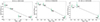 |
Fig. 8. Ratio between observed and theoretical Paschen to Hα flux versus the extinction curve, k(Hα) − k(Pλ), for the three galaxies. The black dashed line represents the linear regression fitting. Every plot is labelled with the AV obtained. |
In Table 1 we present a summary of the results for the different AV values obtained using each method. In general, the AV values derived from the near-IR are lower than those obtained from the UV, as expected when the galaxies are dustier. However, it is important to note that the number of data points used in the near-IR extinction estimation is limited, which can introduce a source of systematic error. A more robust and reliable approach to estimate A(V)Paschen would involve using a larger set of Paschen series lines, particularly when the goal is to correct emission lines spanning the optical to near-IR range. The most remarkable case is ID:50, which shows consistent AV values across the near-IR, optical, and even UV, which is the most uncertain part of the extinction curve, indicating a uniform extinction across the spectrum for this source, clearly matching the assumed extinction curve.
AV values obtained using the three methods.
These discrepancies in the dust correction can be an important source of systematic error, especially when mixing UV and optical lines, as in the calculation of the electron temperature for ID:50 in Section 4.2. For the sake of consistency, we calculated the Hα luminosity (LHα) using the NIRSpec Hα flux from Table B3, corrected using A(V)Balmer. We obtained LHα = (2.070 ± 0.341)×1042 erg/s, which is in very good agreement with the value derived from the SFR estimated via SED fitting (Table B1) using the SFR–LHα relation (Kennicutt et al. 1994; Madau et al. 1998; Kewley & Dopita 2002) applied in Section 3.3, which yields LHα = (2.797 ± 0.397)×1042 erg/s.
4.4. He II ionisation budget
Different ionisation sources have been proposed to explain the origin of the He II excitation. Among them, hot massive stars have been one of the most commonly suggested. In particular, some early-type WR stars with enough Teff are often considered strong candidates, as they are capable of producing photons with energies exceeding 54.4 eV, sufficient to doubly ionise helium (e.g. Schaerer 1996, 2002; Kehrig et al. 2011; Kehrig et al. 2018; Nanayakkara et al. 2019; Mayya et al. 2023). However, WR populations are not expected to be significant in very low-metallicity low-z galaxies (e.g. Guseva et al. 2000; Izotov et al. 1999, 2006; Papaderos et al. 2006; Kehrig et al. 2018), suggesting the need for additional sources of ionisation such as interacting binaries (e.g. Götberg et al. 2017; Smith et al. 2018; Kehrig et al. 2018; Götberg et al. 2019), shocks (e.g. Schaerer et al. 2019; Roy et al. 2025), or X-rays sources (e.g. Schaerer et al. 2019; Saxena et al. 2020; Senchyna et al. 2020). Other types of hot massive stars may contribute more significantly to the global He II ionisation budget in such environments, as WR stars alone cannot fully account for the observed nebular He II emission (e.g. Kehrig et al. 2018; Stanway & Eldridge 2019; Plat et al. 2019; Roy et al. 2025). In particular, in extremely metal-poor galaxies such as IZw18 (Thuan et al. 2004; Kehrig et al. 2015, 2016) and SBS 0335-052E (Hunt et al. 2014; Kehrig et al. 2018), even after accounting for additional ionising sources, it has been necessary to invoke the presence of extremely metal-poor stars with metallicities lower than that of the surrounding gas in order to explain the observed He II budget (extremely metal poor stars with Z ∼ 10−5). These stars are peculiar, extremely hot, and nearly metal-free that can emit large amounts of He+-ionising photons and may boost He II emission in metal-poor galaxies at lower redshifts (e.g. Schaerer 2008; Yoon et al. 2012; Cassata et al. 2013; Kehrig et al. 2018; Pérez-Montero et al. 2020). As Figures 6 and 7 suggest that massive stars could be the main ionising source, we assess whether the photon production from nearly metal-free stars and interacting binaries can reproduce the measured He II photon production by considering the Binary Population and Spectral Synthesis models (BPASSv2.1; Eldridge et al. 2017) models10, which provide a comprehensive set of stellar SEDs that include both single and interacting binary systems (without including x-rays binaries) at very low metallicities (Z = 10−3, 10−4, and 10−5). QHeII can be derived in these models for a given IMF by integrating the SEDs between 1 and 228 Å for instantaneous starburst models with an initial stellar mass of Mini = 106 M⊙ at an age of 106.8 yr, which corresponds to the average age of stellar populations that predominantly produce photons with energies > 54.4 eV (e.g. Nanayakkara et al. 2019; Hawcroft et al. 2025). In Figure 9, we present the values of QHeII derived in Section 3.3 for our He II emitters, plotted against the stellar mass obtained from SED fitting (Table B1), and colour-coded by the gas-phase metallicity derived in Section 3.1. The oblique lines represent the QHeII predictions from the BPASS models, scaled linearly with stellar mass, i.e. if the predicted QHeII is 6.45 × 1048 photons/s for a star cluster of M = 106 M⊙, then a cluster with ten times the stellar mass is expected to produce ten times more ionising photons. We include both models, with interacting binaries (dashed lines) and without them (solid lines), for metallicities Z = 10−3, 10−4, and 10−5. Additionally, we present models adopting a standard Salpeter IMF (Salpeter 1955) with an upper mass limit of Mup = 100 M⊙ (red lines), as well as models assuming a top-heavy IMF with Mup = 300 M⊙ (blue lines).
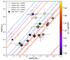 |
Fig. 9. QHeII vs. M⋆ for our sample. The colours correspond to the gas-phase metallicity. The oblique lines represent the QHeII predictions from the BPASS models, scaled linearly with stellar mass. Models with interacting binaries are shown as dashed lines. Those without them are shown as solid lines. In all cases we show the metallicities of Z = 10−3, 10−4, and 10−5. Additionally, we present models adopting a standard Salpeter IMF (Salpeter 1955) with an upper mass limit of |

In general, most of the data points suggest an increase in QHeII as a function of stellar mass (M⋆), along with a trend on gas-phase metallicity.
The comparison with the predictions of BPASS indicate that, for the galaxies with higher gas-phase metallicity (7.7 > 12 + log(O/H) > 7.55) and stellar mass (log(M⋆) ≳ 9 M⊙), the models including single stellar populations with a Salpeter IMF (Mup = 100 M⊙ can reproduce the observed He II ionising photon production when considering nearly metal-free stars (Z⊙/2000 < Z < Z⊙/200). This constraint on stellar metallicity can be relaxed when considering stellar clusters composed of interacting binaries with very low metallicities (Z⊙/200 < Z < Z⊙/20). Thus, both scenarios–single, nearly metal-free stars and very low-metallicity interacting binaries (each with Mup = 100 M⊙)–can account for the observed ionising photon production. However, in the single-star scenario, the stellar metallicity is lower than the gas-phase metallicity. For the binary star models, the stellar metallicity closely matches the gas-phase metallicity only in the highest-metallicity galaxies (7.7 > 12 + log(O/H) > 7.6, which correspond to Zgas ∼ 10−3).
On the other hand, for galaxies in our sample with lower stellar masses and lower gas-phase metallicities than in the previously discussed cases, the first two scenarios cannot fully account for the observed ionising photon production. Instead, a top-heavy IMF with an upper mass limit of Mup = 300 M⊙ must be considered. In this context, both single nearly metal-free stars and very low-metallicity interacting binaries with a top-heavy IMF can reproduce the observed He II-ionising photon production in these low-mass very low-metallicity galaxies. We note that hypothetical rapidly rotating chemically homogeneous evolution (CHE) stars could contribute to enhance UV emission, and therefore to the observed QHeII (Szécsi et al. 2015, 2025; Liu et al. 2025). Analogously, quasi-chemically homogenous evolution (QHE) stars, which are hypothetical main sequence stars evolving to WR stars directly due to their mixing (e.g. Martins et al. 2013; Eldridge et al. 2017), can also contribute to the ionisation budget. Nevertheless, a detailed analysis of the contribution of such stars to the He II ionising budget is beyond the scope of thiswork.
Four cases exhibit even more extreme behaviour (IDs 106, 3621, 8249, and 149), corresponding to the highest QHeII in our sample. The previously discussed scenarios cannot reproduce the observed QHeII values; only models that include nearly metal-free binaries or very low-metallicity binaries with a top-heavy IMF are able to account for the observed ionising photon production. One of the four mentioned cases corresponds to the galaxy with the lowest measured O/H in our sample (ID:149 with 12 + log(O/H) = 7.45). The others lack sufficient signal-to-noise in the [C III] and [O III] lines to allow for a reliable O/H determination (see Section 3.1). These results are similar to those obtained for galaxies such as SBS 0335–052E (marked as a black square in Figure 9) and IZw18, both of which exhibit extremely low metallicities (12 + log(O/H) ≈ 7.2–7.3). In these cases, the observed QHeII can only be reproduced by models that include interacting binaries at Z = 10−5 and a top-heavy IMF in the He II ionisation budget.
It is important to note that the stellar metallicities in the BPASS models are defined in terms of Fe/H, not O/H. Therefore, any direct comparison between stellar and gas-phase metallicity must account for α-enhancement, i.e. the overabundance of α-elements such as oxygen relative to iron (O/Fe), which becomes more pronounced at lower values of 12 + log(O/H) (Steidel et al. 2016; Matteucci 2021; Byrne et al. 2025). Nevertheless, Steidel et al. (2016) have shown that star-forming galaxies at z ∼ 2–3 exhibit emission-line properties indicative of photoionisation by young α-enhanced massive stars, with O/Fe values up to two to five times the solar value. However, this level of enhancement remains insufficient to account for the most extreme cases in our sample, where the stellar metallicity required to reproduce the He II ionisation rate falls in the range Z⊙/2000 < Z < Z⊙/200. In all cases, the gas-phase metallicity need to be lower than the metallicity of the stellar populations to reproduce the observed QHeII, evidencing a decoupling between stellar and gas-phase abundances in high-redshift galaxies (Steidel et al. 2016; Byler et al. 2020), where the ionising stellar populations appear to be more metal-poor than the surrounding gas. This scenario can be attributed with the presence of nearly metal-free very massive stars, and may help explain the rapid enrichment of the ISM in α-elements observed in galaxies with sufficiently high star formation rates. In addition, these findings are similar to previous studies, as the formation of the nebular He II line continues to challenge current stellar models.
5. Summary and conclusions
In this work, we performed a physical and chemical characterisation of a sample of galaxies at z ∼ 2–4 exhibiting prominent nebular He II λ1640 Å emission, commonly referred to as He II emitters. Our sample was selected from the MUSE Hubble Ultra Deep Field surveys (MHUDF; Bacon et al. 2017, 2023), and expanded upon the samples used by previous authors, which include three MUSE fields: the MUSE Extremely Deep Field (MXDF), the Ultra Deep Field survey (UDF-10), and the MOSAIC field. We used the publicly available AMUSED database to identify potential He II emitters.
From a total of 2221 objects in the MHUDF, we identified 25 galaxies exhibiting nebular He II λ1640 Å emission with signal-to-noise ratios greater than 3, spanning a redshift range of 1.907 < z < 4.41. Among these, two are classified as AGNs. For the remaining 23 star-forming galaxies, all cases where the λ = 1214 Å falls within the MUSE range (ten sources excluding the AGNs) show a prominent Lyα emission line.
To complement the MUSE rest-frame UV data, we also incorporated JWST/NIRSpec optical spectra by querying the public DJA database (D’Eugenio et al. 2025). We found that five star-forming galaxies in our sample have publicly available and fully reduced NIRSpec observations.
Using UV-based calibrations, we find that all He II emitters in our sample exhibit very low gas-phase metallicities, with values in the range 7.3 < 12 + log(O/H) < 7.7. Additionally, these galaxies show sub-solar carbon-to-oxygen abundance ratios, with −0.6 < [C/O] < −0.4, similar to those found for other high-redshift He II emitters. In contrast, the nitrogen-to-oxygen ratio remains approximately constant at [N/O] = −0.42, as expected given that nitrogen is primarily produced through secondary nucleosynthesis at higher metallicities. Moreover, the theoretical photoionisation models of Gutkin et al. (2016) predict very low gas-phase metallicities and sub-solar C/O abundance ratios (−0.85 < [C/O] < −0.57). In addition, we derived electron densities using both UV and optical diagnostics, specifically the [C III] λ1907/λ1909 and [S II] λ6716/λ6731 ratios, and found that all galaxies in the sample lie within a diverse low- to intermediate-density regime (102 < ne < 103 cm−3).
To assess the consistency of our calculations and assumptions, we compared dust extinction estimations derived from the UV (using MUSE data) with those obtained in the optical/near-IR (using JWST/NIRSpec data). We found that the AV values derived from the Paschen series in the near-IR are generally lower than those inferred from the UV β slope. This is expected, particularly in galaxies with higher dust content, where the UV slope may overestimate extinction in the optical and near-IR lines. Therefore, in such cases, the β slope should be used exclusively to correct UV fluxes, while the AV derived from the Paschen series is more appropriate for correcting emission lines in the optical/near-IR regime.
A notable exception is object ID:50, which shows uniform extinction across the UV, optical, and near-IR wavelengths. For this galaxy, the extinction-corrected Hα luminosity from NIRSpec is similar to the Hα luminosity inferred from the SED fitting. Given that this object also exhibits the highest number of detected emission lines in the sample, we were able to compute its electron temperature and derive its C/O abundance ratio. The result from the direct method is in very good agreement with the value obtained from the empirical UVcalibration.
We computed the production rates of both H+ and He++ ionising photons and found that QHeII increases exponentially with QHα. Both QHeII and QHα are higher in galaxies with higher stellar masses and greater UV luminosities.
To investigate the origin of the observed He II emission, we compared our results with stellar SED models from BPASS (Eldridge et al. 2017). For our galaxies with higher gas-phase metallicities (7.7 > 12 + log(O/H) > 7.55) and higher stellar mass (log(M⋆) ≳ 9 M⊙), we find that single-star populations with a Salpeter IMF can reproduce the observed QHeII emission, but only if the stars are nearly metal-free (Z⊙/2000 < Z < Z⊙/200). The condition of the metallicity can be relaxed to a very low stellar metallicity (Z⊙/200 < Z < Z⊙/20) when considering binary stars. For our galaxies with lower gas-phase metallicities (12 +log(O/H) ≲ 7.55) and lower stellar masses (log(M⋆) ≲ 9 M⊙), a top-heavy IMF with  = 300 M⊙ is needed to account for the He+ ionisation either assuming single nearly metal-free hot stars or binary stars with lower metallicity than the gas.
In addition to the galaxies discussed above, four galaxies in our sample exhibit higher QHeII values relative to their stellar masses (IDs 106, 3621, 8249, and 149), resembling the well-known extremely metal-poor He II emitters SBS 0335–052E and IZw18 (Kehrig et al. 2015, 2018), especially ID:149 with 12 + log(O/H) = 7.45. Their high observed QHeII can be reproduced either with models that include interacting binaries combined with a top-heavy IMF at Z⊙/200 < Z < Z⊙/20 or with binaries following a Salpeter IMF (Mup = 100 M⊙) at Z⊙/2000 < Z < Z⊙/200 (i.e. nearly metal-free). Notably, one of these four galaxies exhibits the lowest O/H ratio in our sample, further supporting the scenario observed in SBS 0335–052E and IZw18.
In conclusion, the origin of the He II λ1640 Å emission in this sample is influenced by a combination of factors, including stellar mass, IMF, stellar metallicity, and stellar multiplicity. Very hot massive stars can provide sufficient energy to efficiently ionise helium twice; however, in some cases the production of the He+ ionising photons requires nearly metal-free hot stars, a condition that can be relaxed when considering binary stars.
Our analysis, based on a larger and consistently selected sample of galaxies in the MHUDF at the cosmic noon and beyond, indicates that the challenge of reproducing nebular He II emission seem to be a generalised problem in extremely metal poor galaxies.
A significantly larger sample is required to verify these findings and draw more robust conclusions. In future work, we will extend this analysis to a major sample and conduct a more in-depth investigation of Lyman continuum photon escape by examining Lyα line profiles and the two-dimensional spatially extended emission of Lyα, He II, and other detected lines. The galaxy with ID:50 will also be studied as a special case, given its rich set of emission features, spanning from Lyα at 1216 Å to Paγ at 10 938 Å. This offers an extensive dataset that covers a broad spectral range, from the UV with MUSE to the near-infrared with JWST/NIRSpec.
Data availability
The datasets used in this work were obtained from public sources. The MUSE data are available through the Advanced MUSE Data Products (AMUSED) public web interface, which provides access to MUSE datacubes for inspection and retrieval https://amused.univ-lyon1.fr/. The JWST/NIRSpec data were retrieved via DJA web interface https://s3.amazonaws.com/msaexp-nirspec/extractions/nirspec_graded_v2.html. Table B2 is available at the CDS via https://cdsarc.cds.unistra.fr/viz-bin/cat/J/A+A/702/A3.
AMUSED web interface.
In addition to ORIGIN, another algorithm developed by Bacon et al. (2023), called ODHIN, was used to extract spectra from deep-exposure sources. ODHIN is optimised for extracting spectra from blended sources, a common issue in MOSAIC and MXDF, where exposure times exceed 10 hours.
Lyα falls within the MUSE wavelength range for 2.82 ≲ z ≲ 6.64.
grizli pipeline.
msaexp pipeline.
Both cutouts were obtained in the GRIZLI interactive data products interface: https://dawn-cph.github.io/dja/general/mapview/.
MPFIT documentation.
We use the standard notation of [C/O], with the brackets indicating the log of the C/O ratio normalised to the Sun abundance, assuming log(C/O)⊙ = −0.26 (Asplund et al. 2021).
We fix the assumed ne for all galaxies since the emissivity is only weakly dependent on the electron density, only around a 0.5% between 102 and 103 and 1% in the extreme cases of ne = 104 found in Section 3.2.
We use the v2.1 in order to use the “all binary” and “all single” star populations models.
Acknowledgments
The authors acknowledge financial support from the State Agency for Research of the Spanish MCIU through Center of Excellence Severo Ochoa’ award to the Instituto de Astrofísica de Andalucía CEX2021-001131-S funded by MCIN/AEI/10.13039/501100011033, and from the project PID2022-136598NB-C32 “Estallidos8”. R.G.D. acknowledge support by the project ref. AST22_00001_Subp_15 funded from the EU – NextGenerationEU. I.M.C. acknowledges support from ANID programme FONDECYT Postdoctorado 3230653. This work is based in part on observations made with the NASA/ESA/CSA James Webb Space Telescope. The data were obtained from the Mikulski Archive for Space Telescopes at the Space Telescope Science Institute, which is operated by the Association of Universities for Research in Astronomy, Inc., under NASA contract NAS 5-03127 for JWST. The data products presented herein were retrieved from the Dawn JWST Archive (DJA) https://dawn-cph.github.io/dja/. DJA is an initiative of the Cosmic Dawn Center (DAWN), which is funded by the Danish National Research Foundation under grant DNRF140. The authors also acknowledge Roland Bacon for his valuable comments and suggestions, which helped to improve the quality of this manuscript.
References
- Allen, D. A., Wright, A. E., & Goss, W. M. 1976, MNRAS, 177, 91 [NASA ADS] [Google Scholar]
- Allen, M. G., Dopita, M. A., & Tsvetanov, Z. I. 1998, ApJ, 493, 571 [NASA ADS] [CrossRef] [Google Scholar]
- Allen, M. G., Groves, B. A., Dopita, M. A., Sutherland, R. S., & Kewley, L. J. 2008, ApJS, 178, 20 [Google Scholar]
- Amayo, A., Delgado-Inglada, G., & Stasińska, G. 2021, MNRAS, 505, 2361 [CrossRef] [Google Scholar]
- Asplund, M., Amarsi, A. M., & Grevesse, N. 2021, A&A, 653, A141 [NASA ADS] [CrossRef] [EDP Sciences] [Google Scholar]
- Atek, H., Labbé, I., Furtak, L. J., et al. 2024, Nature, 626, 975 [NASA ADS] [CrossRef] [Google Scholar]
- Bacon, R., Conseil, S., Mary, D., et al. 2017, A&A, 608, A1 [NASA ADS] [CrossRef] [EDP Sciences] [Google Scholar]
- Bacon, R., Brinchmann, J., Conseil, S., et al. 2023, A&A, 670, A4 [NASA ADS] [CrossRef] [EDP Sciences] [Google Scholar]
- Bacon, R., Accardo, M., Adjali, L., et al. 2010, in Ground-based and Airborne Instrumentation for Astronomy III, eds. I. S. McLean, S. K. Ramsay, & H. Takami, SPIE Conf. Ser., 7735, 773508 [Google Scholar]
- Bayliss, M. B., Rigby, J. R., Sharon, K., et al. 2014, ApJ, 790, 144 [NASA ADS] [CrossRef] [Google Scholar]
- Berg, D. A., Skillman, E. D., Henry, R. B. C., Erb, D. K., & Carigi, L. 2016, ApJ, 827, 126 [NASA ADS] [CrossRef] [Google Scholar]
- Berg, D. A., Chisholm, J., Erb, D. K., et al. 2019, ApJ, 878, L3 [NASA ADS] [CrossRef] [Google Scholar]
- Berg, D. A., Chisholm, J., Erb, D. K., et al. 2021, ApJ, 922, 170 [CrossRef] [Google Scholar]
- Boogaard, L. A., Brinchmann, J., Bouché, N., et al. 2018, A&A, 619, A27 [NASA ADS] [CrossRef] [EDP Sciences] [Google Scholar]
- Bromm, V. 2013, Rep. Prog. Phys., 76, 112901 [NASA ADS] [CrossRef] [Google Scholar]
- Bruzual, G., & Charlot, S. 2003, MNRAS, 344, 1000 [NASA ADS] [CrossRef] [Google Scholar]
- Bunker, A. J., Saxena, A., Cameron, A. J., et al. 2023, A&A, 677, A88 [NASA ADS] [CrossRef] [EDP Sciences] [Google Scholar]
- Butler, R. E., & Salim, S. 2021, ApJ, 911, 40 [NASA ADS] [CrossRef] [Google Scholar]
- Byler, N., Dalcanton, J. J., Conroy, C., & Johnson, B. D. 2017, ApJ, 840, 44 [Google Scholar]
- Byler, N., Dalcanton, J. J., Conroy, C., et al. 2018, ApJ, 863, 14 [NASA ADS] [CrossRef] [Google Scholar]
- Byler, N., Kewley, L. J., Rigby, J. R., et al. 2020, ApJ, 893, 1 [NASA ADS] [CrossRef] [Google Scholar]
- Byrne, C. M., Eldridge, J. J., & Stanway, E. R. 2025, MNRAS, 537, 2433 [Google Scholar]
- Cai, Z., Fan, X., Jiang, L., et al. 2011, ApJ, 736, L28 [NASA ADS] [CrossRef] [Google Scholar]
- Calzetti, D., Kinney, A. L., & Storchi-Bergmann, T. 1994, ApJ, 429, 582 [Google Scholar]
- Calzetti, D., Armus, L., Bohlin, R. C., et al. 2000, ApJ, 533, 682 [NASA ADS] [CrossRef] [Google Scholar]
- Cardelli, J. A., Clayton, G. C., & Mathis, J. S. 1989, ApJ, 345, 245 [Google Scholar]
- Cassata, P., Le Fèvre, O., Charlot, S., et al. 2013, A&A, 556, A68 [NASA ADS] [CrossRef] [EDP Sciences] [Google Scholar]
- Christensen, L., Laursen, P., Richard, J., et al. 2012, MNRAS, 427, 1973 [NASA ADS] [CrossRef] [Google Scholar]
- de Graaff, A., Brammer, G., Weibel, A., et al. 2025, A&A, 697, A189 [NASA ADS] [CrossRef] [EDP Sciences] [Google Scholar]
- del Moral-Castro, I., Vílchez, J. M., Iglesias-Páramo, J., & Arroyo-Polonio, A. 2024, A&A, 688, A28 [NASA ADS] [CrossRef] [EDP Sciences] [Google Scholar]
- D’Eugenio, F., Cameron, A. J., Scholtz, J., et al. 2025, ApJS, 277, 4 [Google Scholar]
- Dopita, M. A., Sutherland, R. S., Nicholls, D. C., Kewley, L. J., & Vogt, F. P. A. 2013, ApJS, 208, 10 [NASA ADS] [CrossRef] [Google Scholar]
- Drake, A. B., Garel, T., Wisotzki, L., et al. 2017, A&A, 608, A6 [NASA ADS] [CrossRef] [EDP Sciences] [Google Scholar]
- Eldridge, J. J., & Stanway, E. R. 2012, MNRAS, 19, 479 [Google Scholar]
- Eldridge, J. J., & Stanway, E. R. 2022, ARA&A, 60, 455 [NASA ADS] [CrossRef] [Google Scholar]
- Eldridge, J. J., Stanway, E. R., Xiao, L., et al. 2017, PASA, 34, e058A [Google Scholar]
- Erb, D. K., Pettini, M., Shapley, A. E., et al. 2010, ApJ, 719, 1168 [Google Scholar]
- Feltre, A., Charlot, S., & Gutkin, J. 2016, MNRAS, 456, 3354 [Google Scholar]
- Feltre, A., Bacon, R., Tresse, L., et al. 2018, A&A, 617, A62 [NASA ADS] [CrossRef] [EDP Sciences] [Google Scholar]
- Ferland, G. J., Porter, R. L., van Hoof, P. A. M., et al. 2013, Rev. Mexicana Astron. Astrofis., 49, 137 [Google Scholar]
- Finkelstein, S. L., D’Aloisio, A., Paardekooper, J.-P., et al. 2019, ApJ, 879, 36 [Google Scholar]
- Fitzpatrick, E. L., & Massa, D. 1990, ApJS, 72, 163 [NASA ADS] [CrossRef] [Google Scholar]
- Fitzpatrick, E. L., & Massa, D. 2007, ApJ, 663, 320 [Google Scholar]
- Fitzpatrick, E. L., & Massa, D. 2009, ApJ, 699, 1209 [CrossRef] [Google Scholar]
- Garnett, D. R., Kennicutt, R. C., Jr, Chu, Y.-H., & Skillman, E. D. 1991, ApJ, 373, 458 [NASA ADS] [CrossRef] [Google Scholar]
- Garnett, D. R., Skillman, E. D., Dufour, R. J., et al. 1995, ApJ, 443, 64 [Google Scholar]
- González-Díaz, R., Rosales-Ortega, F. F., Galbany, L., et al. 2024, A&A, 687, A20 [NASA ADS] [CrossRef] [EDP Sciences] [Google Scholar]
- Götberg, Y., de Mink, S. E., & Groh, J. H. 2017, A&A, 608, A11 [NASA ADS] [CrossRef] [EDP Sciences] [Google Scholar]
- Götberg, Y., de Mink, S. E., Groh, J. H., Leitherer, C., & Norman, C. 2019, A&A, 629, A134 [NASA ADS] [CrossRef] [EDP Sciences] [Google Scholar]
- Götberg, Y., Drout, M. R., Ji, A. P., et al. 2023, ApJ, 959, 125 [CrossRef] [Google Scholar]
- Groves, B. A., Dopita, M. A., & Sutherland, R. S. 2004, ApJS, 153, 75 [NASA ADS] [CrossRef] [Google Scholar]
- Guseva, N. G., Izotov, Y. I., & Thuan, T. X. 2000, ApJ, 531, 776 [NASA ADS] [CrossRef] [Google Scholar]
- Gutkin, J., Charlot, S., & Bruzual, G. 2016, MNRAS, 462, 1757 [Google Scholar]
- Hawcroft, C., Leitherer, C., Arangure, O., et al. 2025, arXiv e-prints [arXiv:2505.24841] [Google Scholar]
- Heintz, K. E., Watson, D., Brammer, G., et al. 2024, Science, 384, 890 [NASA ADS] [CrossRef] [Google Scholar]
- Hunt, L. K., Testi, L., Casasola, V., et al. 2014, A&A, 561, A49 [NASA ADS] [CrossRef] [EDP Sciences] [Google Scholar]
- Iani, E., Zanella, A., Vernet, J., et al. 2023, MNRAS, 518, 5018 [Google Scholar]
- Izotov, Y. I., & Thuan, T. X. 2004, ApJ, 602, 200 [CrossRef] [Google Scholar]
- Izotov, Y. I., Chaffee, F. H., Foltz, C. B., et al. 1999, ApJ, 527, 757 [NASA ADS] [CrossRef] [Google Scholar]
- Izotov, Y. I., Schaerer, D., Blecha, A., et al. 2006, A&A, 459, 71 [NASA ADS] [CrossRef] [EDP Sciences] [Google Scholar]
- James, B. L., Pettini, M., Christensen, L., et al. 2014, MNRAS, 440, 1794 [NASA ADS] [CrossRef] [Google Scholar]
- Jaskot, A. E., & Ravindranath, S. 2016, ApJ, 833, 136 [NASA ADS] [CrossRef] [Google Scholar]
- Johnson, B. D., Leja, J., Conroy, C., & Speagle, J. S. 2021, ApJS, 254, 22 [NASA ADS] [CrossRef] [Google Scholar]
- Keenan, F. P., Feibelman, W. A., & Berrington, K. A. 1992, ApJ, 389, 443 [NASA ADS] [CrossRef] [Google Scholar]
- Kehrig, C., Oey, M. S., Crowther, P. A., et al. 2011, A&A, 526, A128 [NASA ADS] [CrossRef] [EDP Sciences] [Google Scholar]
- Kehrig, C., Vílchez, J. M., Telles, E., Cuisinier, F., & Pérez-Montero, E. 2006, A&A, 457, 477 [NASA ADS] [CrossRef] [EDP Sciences] [Google Scholar]
- Kehrig, C., Vílchez, J. M., Pérez-Montero, E., et al. 2015, ApJ, 801, L28 [NASA ADS] [CrossRef] [Google Scholar]
- Kehrig, C., Vílchez, J. M., Pérez-Montero, E., et al. 2016, MNRAS, 459, 2992 [NASA ADS] [CrossRef] [Google Scholar]
- Kehrig, C., Vílchez, J. M., Guerrero, M. A., et al. 2018, MNRAS, 480, 1081 [NASA ADS] [Google Scholar]
- Kehrig, C., Guerrero, M. A., Vílchez, J. M., & Ramos-Larios, G. 2021, ApJ, 908, L54 [NASA ADS] [CrossRef] [Google Scholar]
- Kennicutt, R. C., Jr, Tamblyn, P., & Congdon, C. E. 1994, ApJ, 435, 22 [NASA ADS] [CrossRef] [Google Scholar]
- Kewley, L. J., & Dopita, M. A. 2002, ApJS, 142, 35 [Google Scholar]
- Kojima, T., Ouchi, M., Nakajima, K., et al. 2017, PASJ, 69, 44 [NASA ADS] [CrossRef] [Google Scholar]
- Le Fèvre, O., Vettolani, G., Maccagni, D., et al. 2003, The Messenger, 111, 18 [NASA ADS] [Google Scholar]
- Lennon, D. J., & Burke, V. M. 1994, A&AS, 103, 273 [NASA ADS] [Google Scholar]
- Lilly, S. J., Tresse, L., Hammer, F., Crampton, D., & Le Fevre, O. 1995, ApJ, 455, 108 [NASA ADS] [CrossRef] [Google Scholar]
- Liu, B., Sibony, Y., Meynet, G., & Bromm, V. 2025, ApJ, 980, L30 [Google Scholar]
- Luridiana, V., Morisset, C., & Shaw, R. A. 2015, A&A, 573, A42 [NASA ADS] [CrossRef] [EDP Sciences] [Google Scholar]
- Madau, P., Ferguson, H. C., Dickinson, M. E., et al. 1996, MNRAS, 283, 1388 [Google Scholar]
- Madau, P., Pozzetti, L., & Dickinson, M. 1998, ApJ, 498, 106 [NASA ADS] [CrossRef] [Google Scholar]
- Martins, F., Depagne, E., Russeil, D., & Mahy, L. 2013, A&A, 554, A23 [NASA ADS] [CrossRef] [EDP Sciences] [Google Scholar]
- Mary, D., Bacon, R., Conseil, S., Piqueras, L., & Schutz, A. 2020, A&A, 635, A194 [EDP Sciences] [Google Scholar]
- Matteucci, F. 2021, A&A Rev., 29, 5 [NASA ADS] [CrossRef] [Google Scholar]
- Mayya, Y. D., Carrasco, E., Gómez-González, V. M. A., et al. 2020, MNRAS, 498, 1496 [NASA ADS] [CrossRef] [Google Scholar]
- Mayya, Y. D., Plat, A., Gómez-González, V. M. A., et al. 2023, MNRAS, 519, 5492 [NASA ADS] [CrossRef] [Google Scholar]
- Meurer, G. R., Heckman, T. M., & Calzetti, D. 1999, ApJ, 521, 64 [Google Scholar]
- Mondal, C., Saha, K., Borgohain, A., et al. 2025, ApJ, 988, 171 [Google Scholar]
- Nagao, T., Maiolino, R., & Marconi, A. 2006, A&A, 447, 863 [NASA ADS] [CrossRef] [EDP Sciences] [Google Scholar]
- Nakajima, K., & Maiolino, R. 2022, MNRAS, 513, 5134 [NASA ADS] [CrossRef] [Google Scholar]
- Nanayakkara, T., Brinchmann, J., Boogaard, L., et al. 2019, A&A, 624, A89 [NASA ADS] [CrossRef] [EDP Sciences] [Google Scholar]
- Nicholls, D. C., Kewley, L. J., & Sutherland, R. S. 2020, PASP, 132, 033001 [NASA ADS] [CrossRef] [Google Scholar]
- Osterbrock, D. E., & Ferland, G. J. 2006, Astrophysics of Gaseous Nebulae and Active Galactic nuclei (Sausalito, CA: University Science Books) [Google Scholar]
- Papaderos, P., Izotov, Y. I., Guseva, N. G., Thuan, T. X., & Fricke, K. J. 2006, A&A, 454, 119 [NASA ADS] [CrossRef] [EDP Sciences] [Google Scholar]
- Pérez-Montero, E., & Amorín, R. 2017, MNRAS, 467, 1287 [Google Scholar]
- Pérez-Montero, E., Kehrig, C., Vílchez, J. M., et al. 2020, A&A, 643, A80 [NASA ADS] [CrossRef] [EDP Sciences] [Google Scholar]
- Plat, A., Charlot, S., Bruzual, G., et al. 2019, MNRAS, 490, 978 [Google Scholar]
- Proxauf, B., Öttl, S., & Kimeswenger, S. 2014, A&A, 561, A10 [NASA ADS] [CrossRef] [EDP Sciences] [Google Scholar]
- Roy, A., Sutherland, R. S., Krumholz, M. R., Heger, A., & Dopita, M. A. 2020, MNRAS, 494, 3861 [Google Scholar]
- Roy, A., Krumholz, M. R., Salvadori, S., et al. 2025, A&A, 696, A29 [NASA ADS] [CrossRef] [EDP Sciences] [Google Scholar]
- Salpeter, E. E. 1955, ApJ, 121, 161 [Google Scholar]
- Saxena, A., Pentericci, L., Mirabelli, M., et al. 2020, A&A, 636, A47 [NASA ADS] [CrossRef] [EDP Sciences] [Google Scholar]
- Schaerer, D. 1996, ApJ, 467, L17 [NASA ADS] [CrossRef] [Google Scholar]
- Schaerer, D. 2002, A&A, 382, 28 [NASA ADS] [CrossRef] [EDP Sciences] [Google Scholar]
- Schaerer, D. 2008, in Low-Metallicity Star Formation: From the First Stars to Dwarf Galaxies, eds. L. K. Hunt, S. C. Madden, & R. Schneider, IAU Symp., 255, 66 [Google Scholar]
- Schaerer, D., Fragos, T., & Izotov, Y. I. 2019, A&A, 622, L10 [NASA ADS] [CrossRef] [EDP Sciences] [Google Scholar]
- Senchyna, P., Stark, D. P., Mirocha, J., et al. 2020, MNRAS, 494, 941 [CrossRef] [Google Scholar]
- Shirazi, M., & Brinchmann, J. 2012, MNRAS, 421, 1043 [NASA ADS] [CrossRef] [Google Scholar]
- Smith, N., Götberg, Y., & de Mink, S. E. 2018, MNRAS, 475, 772 [NASA ADS] [CrossRef] [Google Scholar]
- Soto, K. T., Lilly, S. J., Bacon, R., Richard, J., & Conseil, S. 2016, MNRAS, 458, 3210 [Google Scholar]
- Stanway, E. R., & Eldridge, J. J. 2019, A&A, 621, A105 [NASA ADS] [CrossRef] [EDP Sciences] [Google Scholar]
- Stark, D. P., Ellis, R. S., Charlot, S., et al. 2017, MNRAS, 464, 469 [NASA ADS] [CrossRef] [Google Scholar]
- Steidel, C. C., Strom, A. L., Pettini, M., et al. 2016, ApJ, 826, 159 [NASA ADS] [CrossRef] [Google Scholar]
- Szécsi, D., Langer, N., Yoon, S.-C., et al. 2015, A&A, 581, A15 [NASA ADS] [CrossRef] [EDP Sciences] [Google Scholar]
- Szécsi, D., Tramper, F., Kubátová, B., et al. 2025, A&A, in press, https://doi.org/10.1051/0004-6361/202452483 [Google Scholar]
- Thuan, T. X., Bauer, F. E., Papaderos, P., & Izotov, Y. I. 2004, ApJ, 606, 213 [NASA ADS] [CrossRef] [Google Scholar]
- Topping, M. W., Stark, D. P., Senchyna, P., et al. 2024, MNRAS, 529, 3301 [NASA ADS] [CrossRef] [Google Scholar]
- Tumlinson, J., & Shull, J. M. 2000, ApJ, 528, L65 [NASA ADS] [CrossRef] [Google Scholar]
- Valentino, F., Brammer, G., Gould, K. M. L., et al. 2023, ApJ, 947, 20 [NASA ADS] [CrossRef] [Google Scholar]
- Venditti, A., Bromm, V., Finkelstein, S. L., et al. 2024, ApJ, 973, L12 [NASA ADS] [CrossRef] [Google Scholar]
- Villar-Martin, M., Tadhunter, C., & Clark, N. 1997, A&A, 323, 21 [Google Scholar]
- Villar-Martín, M., Cerviño, M., & González Delgado, R. M. 2004, MNRAS, 355, 1132 [CrossRef] [Google Scholar]
- Wise, J. H., Turk, M. J., Norman, M. L., & Abel, T. 2012, ApJ, 745, 50 [NASA ADS] [CrossRef] [Google Scholar]
- Wise, J. H., Demchenko, V. G., Halicek, M. T., et al. 2014, MNRAS, 442, 2560 [NASA ADS] [CrossRef] [Google Scholar]
- Xiao, L., Stanway, E. R., & Eldridge, J. J. 2018, MNRAS, 477, 904 [Google Scholar]
- Yoon, S. C., Dierks, A., & Langer, N. 2012, A&A, 542, A113 [NASA ADS] [CrossRef] [EDP Sciences] [Google Scholar]
- Yuan, T. T., & Kewley, L. J. 2009, ApJ, 699, L161 [Google Scholar]
- Zhou, L., Shi, Y., Zhang, Z.-Y., & Wang, J. 2021, A&A, 653, L10 [NASA ADS] [CrossRef] [EDP Sciences] [Google Scholar]
Appendix A: He II emitters spectra
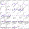 |
Fig. A.1. He II emitters sample ordered by S/N(He II ). The blue and red spectra represent the reference spectrum and the model continuum + fit, respectively. The S/N of He II and Lyα (when detected) are included in the labels. The last two panels correspond to the two AGNs identified in the sample, exhibiting broad He II and C IV 1548,51 Å lines. |
Appendix B: Additional tables
General characteristics of the He II emitters sample.
Sample UV lines fluxes measured with MUSE.
He II emitters NIRSpec sample.
He II emitters main results.
Appendix C: Flux comparison
As a sanity check, we compared our measured fluxes for the five He II emitters in common with Nanayakkara et al. (2019) (IDs: 1024, 1036, 1045, 1273, and 3621). In Figure we show this comparison for the matched detections, considering only the emission lines with a S/N greater than 3. In general, our fluxes are in good agreement.
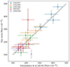 |
Fig. B.1. Comparison between the fluxes used in this work (when the target S/N is reached) and the fluxes obtained by Nanayakkara et al. (2019) in their work for the same objects. The diagonal dashed line indicates the 1:1 relation, showing that our fluxes are in excellent agreement. |
All Tables
All Figures
|
Fig. 1. Example of a detected source from MHUDF, representing the galaxy with ID 106 in the MXDF. Upper panels: MUSE white-light image (left), ORIGIN segmentation map of the source (centre), and HST F606W filter image (right). Lower pannel: Observed reference spectrum of the source extracted with ORIGIN (blue) and its respective continuum + emission line fit (red). |
| In the text | |
|
Fig. 2. Stellar mass vs. star formation rate for the sample, derived from the SED reported in the AMUSED database (Bacon et al. 2023), colour-coded by redshift and excluding the two AGNs. The z = 3 SFMS, as derived by Boogaard et al. (2018), is represented by a dashed blue line. The sample shows a slight offset relative to the z = 3 SFMS, but follows the expected linear trend. |
| In the text | |
|
Fig. 3. Reduced 2D and 1D NIRSpec spectrum of the galaxy with ID:50 at z = 3.325, obtained using the G235M/F170LP grating–filter combination. The right panels display a NIRCam RGB cutout of the galaxy, constructed using the F115W, F277W, and F444W filters (top), and a F444W cutout with the NIRSpec slit location overplotted in magenta (bottom). Both NIRCam cutouts were obtained from the GRIZLI public database. |
| In the text | |
|
Fig. 4. He2-O3C3 diagnosis diagram. The red lines represent the polynomial from equation (2) at 12 + log10(O/H) = 7.3, 7.5, and 7.7 respectively. The colours indicate stellar mass, while the open points correspond to galaxies without SED information, and consequently no measured M⋆. Only 18 points are shown as the rest present a S/N lower than 3 in at least one of the involved emission lines. All galaxies fall within a metal-poor regime; three of them approach the extremely metal-poor regime (12 + log(O/H) ≈ 7.3), showing a trend with M⋆. |
| In the text | |
|
Fig. 5. He++ vs. H+ ionising photon production, derived from Equations (5) and (6). The colours indicate the stellar mass of each galaxy. The black square represents measurements for the extremely metal-poor star-forming galaxy SBS 0335-052E taken from Kehrig et al. (2018). |
| In the text | |
|
Fig. 6. QHeII in units of log(photons/s) as a function of UV magnitude (left panel) and of stellar mass (right panel). The colours indicate the stellar mass of each galaxy. The relationship between the two ionising photon production rates appears to be exponential, with both quantities increasing as a function of stellar mass. |
| In the text | |
|
Fig. 7. Left: [C III] λ1907/He II – [O III] λ1666/He II diagnosis. The Gutkin et al. (2016) models plotted correspond to a pure photoionisation scenario due to massive stars with log(Us) = − 1, ξd = 0.1, mup = 300 M⊙, and |
| In the text | |
|
Fig. 8. Ratio between observed and theoretical Paschen to Hα flux versus the extinction curve, k(Hα) − k(Pλ), for the three galaxies. The black dashed line represents the linear regression fitting. Every plot is labelled with the AV obtained. |
| In the text | |
|
Fig. 9. QHeII vs. M⋆ for our sample. The colours correspond to the gas-phase metallicity. The oblique lines represent the QHeII predictions from the BPASS models, scaled linearly with stellar mass. Models with interacting binaries are shown as dashed lines. Those without them are shown as solid lines. In all cases we show the metallicities of Z = 10−3, 10−4, and 10−5. Additionally, we present models adopting a standard Salpeter IMF (Salpeter 1955) with an upper mass limit of |
| In the text | |
|
Fig. A.1. He II emitters sample ordered by S/N(He II ). The blue and red spectra represent the reference spectrum and the model continuum + fit, respectively. The S/N of He II and Lyα (when detected) are included in the labels. The last two panels correspond to the two AGNs identified in the sample, exhibiting broad He II and C IV 1548,51 Å lines. |
| In the text | |
|
Fig. B.1. Comparison between the fluxes used in this work (when the target S/N is reached) and the fluxes obtained by Nanayakkara et al. (2019) in their work for the same objects. The diagonal dashed line indicates the 1:1 relation, showing that our fluxes are in excellent agreement. |
| In the text | |
Current usage metrics show cumulative count of Article Views (full-text article views including HTML views, PDF and ePub downloads, according to the available data) and Abstracts Views on Vision4Press platform.
Data correspond to usage on the plateform after 2015. The current usage metrics is available 48-96 hours after online publication and is updated daily on week days.
Initial download of the metrics may take a while.