| Issue |
A&A
Volume 702, October 2025
|
|
|---|---|---|
| Article Number | A175 | |
| Number of page(s) | 9 | |
| Section | Cosmology (including clusters of galaxies) | |
| DOI | https://doi.org/10.1051/0004-6361/202555952 | |
| Published online | 17 October 2025 | |
X-ray flux–mass relation for z ≳ 0.7 galaxy clusters
1
Space Research Institute (IKI), Profsoyuznaya 84/32, Moscow 117997, Russia
2
Max Planck Institute for Astrophysics, Karl-Schwarzschild-Str. 1, D-85741 Garching, Germany
3
Universitäts-Sternwarte, Fakultät für Physik, Ludwig-Maximilians-Universität München, Scheinerstr. 1, 81679 München, Germany
⋆ Corresponding author: This email address is being protected from spambots. You need JavaScript enabled to view it.
Received:
15
June 2025
Accepted:
5
August 2025
Abstract
We use a subsample of co-detections of the ACT and MaDCoWS cluster catalogs to verify the predicted relation between the observed X-ray flux FX in the 0.5−2 keV band and the cluster mass M500c for halos at z > 0.6 − 0.7. We modified this relation by introducing a correction coefficient, η, which is supposed to encapsulate factors associated with a particular method of flux estimation, the sample selection function, the definition of the cluster mass. We show that the X-ray flux, being the most basic X-ray observable, serves as a convenient and low-cost mass indicator for distant galaxy clusters with photometric or even missing redshifts (by setting z = 1) as long as it is known that z ≳ 0.6 − 0.7. The correction coefficient η is ≈0.8 if MUPP500c from the ACT-DR5 catalog are used as cluster masses, whereas η ≈ 1.1 if weak-lensing-calibrated masses MCal500c are used instead.
Key words: X-rays: galaxies: clusters
© The Authors 2025
 Open Access article, published by EDP Sciences, under the terms of the Creative Commons Attribution License (https://creativecommons.org/licenses/by/4.0), which permits unrestricted use, distribution, and reproduction in any medium, provided the original work is properly cited.
This article is published in open access under the Subscribe to Open model. This email address is being protected from spambots. You need JavaScript enabled to view it. to support open access publication.
1. Introduction
In the current paradigm of structure formation, galaxy clusters are formed through the gravitational collapse of the highest (and rarest) density peaks in the primordial density field. Thus, the abundance of clusters (as a function of redshift) carries the imprint of the growth of the structure over cosmological time and, as a consequence, serves as a sensitive probe of the underlying cosmological parameters (for reviews see, e.g., Allen et al. 2011; Kravtsov & Borgani 2012; Pratt et al. 2019). Over the past several decades, multiwavelength observations of galaxy clusters have been a major focus of research. Clusters can be efficiently detected in optical, X-ray, and Sunyaev-Zeldovich (SZ; Sunyaev & Zeldovich 1972) effect observations. Numerous galaxy cluster surveys have delivered (and will be delivering) large samples of cluster candidates based on different observational proxies, such surveys include those from the Dark Energy Spectroscopic Instrument (DESI Collaboration 2016), the eROSITA telescope on board the SRG observatory (Sunyaev et al. 2021; Predehl et al. 2021), and Atacama Cosmology Telescope (ACT; Swetz et al. 2011), to name a few. The main scientific driver for these surveys is to constrain cosmological parameters by measuring the cluster mass function, for which reliable mass measurements for clusters are necessary. Numerical simulations can predict the abundance of massive halos (e.g., Sheth et al. 2001; Jenkins et al. 2001; Tinker et al. 2008; Warren et al. 2006) while taking into account background cosmology and additional effects, for example, active galactic nuclei (AGNs) feedback. While different cluster properties can be predicted, most often the mass function is used as a compact proxy of cosmological parameters, such as the amplitude of perturbations at scales of ∼10 Mpc or the growth factor as a function of z. For a fair comparison, the cluster mass function would ideally be derived from observations. However, the mass cannot be measured directly. Therefore, scaling relations between the cluster mass and observable properties are often relied on, such as optical richness, velocity dispersion, integrated Compton-y parameter, X-ray luminosity, gas temperature, and gas mass. (e.g., Giodini et al. 2013). Also ideally, one would have an observable (or a set of observables) that are (1) easy to measure, (2) accessible for large samples of clusters (i.e., no additional observations are required), (3) tightly related to the total cluster mass, and (4) have a low scatter. Another useful observable would be an observable that is readily available and can be used for a preselection of cluster samples for deeper studies. This is the main focus of the present study, with the observed X-ray flux taking the role of such an observable.
Cluster masses could be determined from, for example, a weak lensing (WL) analysis. Currently, such an analysis is considered to be one of the least biased methods to measure the total masses of massive clusters Mantz et al. (2016), Umetsu (2020), Oguri & Miyazaki (2025). However, there are still inherent systematic errors (e.g., triaxiality, projection effects, and miscentering; Massey et al. 2013), and from the observational point of view, WL requires large-area observations of background galaxies.
Most commonly, cluster masses are inferred from X-ray and SZ observations. The total SZ flux is expected to correlate tightly with the total cluster mass (e.g., Nagai 2006; Arnaud et al. 2010; Planck Collaboration III 2013). X-ray observations of hot intracluster gas provide information about gas temperature and density profiles, enabling the determination of individual cluster masses under the assumption of hydrostatic equilibrium. However, such detailed X-ray observations are not feasible for large samples of clusters, and for shallow surveys, global cluster properties such as X-ray luminosity or temperature and gas mass can be used to estimate the total mass. Among X-ray mass proxies, YX = MgasT, which is a product of gas mass and X-ray spectroscopic temperature, is believed to have the lowest scatter (Kravtsov et al. 2006). However, when data quality does not permit the determination of the temperature of a cluster, possibly less accurate but easier to measure observables have to be relied on, such as X-ray luminosity (e.g., Pratt et al. 2009, 2022; Mantz et al. 2018) or flux (Churazov et al. 2015) or the average energy of the X-ray spectrum – an alternative to X-ray temperature for low-redshift clusters suggested in Kruglov et al. (2025). In this work, we focus on a sample of high-redshift (z > 0.7) galaxy clusters (Orlowski-Scherer et al. 2021) with SZ-based mass measurements and take advantage of the all-sky SRG/eROSITA survey data to verify and calibrate the scaling relation between the cluster mass and the X-ray flux. The latter is the most direct X-ray observable, which can be used for mass estimates even if redshift is not known (for distant objects).
This paper is organized as follows: Section 2 provides a description of the data and catalogs we use. In Section 3, we present the baseline relation between the cluster mass and the X-ray flux and how eROSITA X-ray fluxes are measured. Next, we calibrate the FX − M500c relation in Section 4 and summarize the obtained results in Section 5.
This work relies on X-ray scaling relations obtained in Vikhlinin et al. (2009) and Churazov et al. (2015). For consistency, we adopted the same set of cosmological parameters as in Churazov et al. (2015): ΩM = 0.27, ΩΛ = 0.73, and h = 0.7. Throughout the paper, a cluster mass refers to M500c, which is defined within the radius R500c enclosing the average mass density of 500 times the critical density at a cluster redshift.
2. Data sets
2.1. eROSITA data preparation
We used the data obtained with the eROSITA telescope (Predehl et al. 2021) on board the SRG observatory (Sunyaev et al. 2021) accumulated over four consecutive all-sky surveys. The initial reduction and processing of the data were performed at IKI using standard routines of the eSASS software (Brunner et al. 2018; Predehl et al. 2021) and proprietary software developed in the RU eROSITA consortium, while the imaging and spectral analysis were carried out with the background modeling, vignetting, point spread function, and spectral response function calibrations built upon the standard ones via slight modifications motivated by results of calibration and performance verification observations (e.g., Churazov et al. 2021; Khabibullin et al. 2023).
2.2. SZ cluster catalogs
Recently, a large catalog of Sunyaev-Zel’dovich (SZ) selected galaxy clusters surveyed by ACT has been published by Hilton et al. (2021). The ACT DR5 catalog provides cluster mass estimates, M500c, derived from an SZ signal for a large sample of clusters. At the redshift range of our interest, z > 0.7, there are 364 clusters with the Galactic longitude 0° < l < 180° and with available SZ-based masses. As a mass proxy, we used values of  (the column M500c in the ACT DR5 catalog) that were obtained by assuming the universal pressure profile and the scaling relation between an SZ signal and a cluster mass from Arnaud et al. (2010). Hilton et al. (2021) have also reported
  (the column M500cCal) masses rescaled using the richness-based weak-lensing mass calibration, where
  (Hilton et al. 2021).
For the calibration of the relation between an X-ray flux and a cluster mass, we made use of a catalog from Orlowski-Scherer et al. (2021), which consists of clusters detected both in the Massive and Distant Clusters of WISE Survey (MaDCoWS; Gonzalez et al. 2019) and ACT data. Keeping objects with the galactic longitude 0° < l < 180° and z ≥ 0.7 yielded 36 clusters. The cluster masses obtained in Orlowski-Scherer et al. (2021) are essentially identical to the  values from Hilton et al. (2021).
3. X-ray flux as the mass proxy
3.1. FX–M500c relation
Churazov et al. (2015) showed that for z > 0.6, there is a relatively tight correlation between the observed X-ray flux in the 0.5−2.0 keV energy range and the cluster mass M500c:
 (1)
(1)
The above expression is based on the X-ray scaling relations in Vikhlinin et al. (2009), with its tightness resulting from the evolution of cluster properties with redshift. We used it as a baseline to derive a simple recipe for estimating galaxy cluster masses from eROSITA data. We patched the relation (1) with a weak dependence on the redshift and added a correction coefficient, η, that is supposed to encapsulate factors associated with, for example, a particular method of flux estimation, the sample selection function, and the definition of the mass. The modified FX − M500c relation thus reads as
 (2)
(2)
The scaling relations of Vikhlinin et al. (2009) were derived from the analysis of X-ray selected clusters with masses M500c ≳ 1.5 × 10¹⁴ M⊙ at z = 0.02 − 0.9. We considered a similar mass range and assumed that the scaling relations hold for 0.7 < z < 2. The factor z0.5 might improve the tightness of the relation (1) (see Fig. 4 in Churazov et al. 2015 and Appendix A), unless it is subdominant to the observational or intrinsic scatter in the properties of the clusters. This factor can be omitted for crude mass estimates, which is the main purpose of this procedure.
3.2. X-ray flux estimation
Even the most massive clusters at redshift z ∼ 1 are expected to be relatively faint X-ray sources, with the flux ≲a few × 10−13 erg s−1 cm−2 in 0.5−2 keV (e.g., Churazov et al. 2015, their Fig. 3), so with a shallow exposure of the eROSITA all-sky survey, at most ∼100 counts are expected to be detected from them. Although this is well above the commonly accepted detection limits due to pure statistical (Poisson) and background fluctuations, the robust characterization of faint extended sources is more challenging. Moreover, the diffuse X-ray emission from galaxy clusters can be contaminated by an (unresolved) AGN, which makes flux measurements via simple fitting strongly dependent on the spatial model assumptions. Instead, we measured X-ray fluxes from a fixed aperture. Such an approach is model independent, simple in use, and fast, but not without its own flaws, which we discuss in Appendix B.
Assuming the Tinker mass function (Tinker et al. 2008), we estimated that the top most massive 100 clusters at z ≥ 0.7 have masses M500c ∼ 6.5 × 10¹⁴ M⊙. The angular sizes of the R500c regions, where the bulk of the X-ray emission is expected to be concentrated, are ∼2.4′. For comparison, for the most massive 100 clusters at z ≥ 1, M500c ∼ 4.5 × 10¹⁴ M⊙ and R500c ∼ 1.6′. Below, we estimate the X-ray flux from galaxy clusters using a circular aperture with fixed size; we set its radius to r = 2′.
First, we measured the 0.4−2.3 keV count rate within a circle with radius r = 2′ centered at the cluster position. The local X-ray background signal was estimated in a ring with 6′< r < 20′ (see Fig. 1 for an illustration). To reduce scatter in the flux estimates associated with the cosmic X-ray background (CXB), we detected and masked bright sources using flux cuts discussed in the following sections. The detection and characterization of sources were performed in the same way as in Churazov et al. (2021), Khabibullin et al. (2023), where special care was taken to separate the extended diffuse emission from the point or mildly extended sources. Next, the extracted count rates within the source apertures were corrected for the background contributions and converted to the 0.5−2 keV flux using the constant factor, which is suitable for extragalactic sources with hot thermal spectrum and small absorbing column density (e.g., Lyskova et al. 2023). The resulting flux was further corrected for the excess in the resolved CXB fraction in the background region compared to the source aperture (see Appendix B). Such a correction is needed if there is a non-negligible bias arising from different flux cuts applied to source and background regions.
 |
Fig. 1. Sunyaev-Zel’dovich and X-ray views on the galaxy cluster ACT-CL J0105.8−1839. Left panel: Planck + ACT Compton-y map (Coulton et al. 2024). Middle panel: eROSITA 0.4−2.3 keV image. We used a ring with 6′< R < 20′ to estimate the background, and it was then subtracted from the source region (marked as a white circle). The right panel illustrates the source removal procedure. |
4. Calibration of the FX − M500c relation
4.1. ACT/MaDCoWS sample
We calibrated the relation (2) with and without the z dependence using a subsample of ACT/MaDCoWS co-detections from Orlowski-Scherer et al. (2021) with z > 0.7 (see Section 2.2). From both the source and background regions, we masked bright sources with the 0.5−2 keV flux above 10−13 erg s−1 cm−2. Such sources are rare but introduce a large scatter to flux estimates. Additionally, in the background region, we masked all the detected sources down to 0.5−2 keV flux of ∼2 × 10⁻¹⁴ erg s−1 cm−2. We did not apply this flux cut to the source region since weak sources could not be unambiguously detected in the area dominated by a cluster emission (see a discussion in Appendix B). Therefore, the obtained source flux, corrected for the background contribution, needs to be further corrected for the excess in the resolved CXB fraction in the background region compared to the source aperture (see column “B1 (mean)” for the sample of 36 objects in Table B.1). We calculated flux uncertainties accounting for a Poisson noise σstat (count statistics) and for the average variance in the background region in the 0.5−2 keV energy range (with the standard deviation σvar = 1.5 × 10⁻¹⁴ erg s−1 cm−2). Figure 2 shows the resulting eROSITA fluxes in the 0.5−2 keV energy range, masses M500c, and redshifts for our subsample of clusters. The subsample of the Orlowski-Scherer et al. (2021) catalog used here includes clusters with masses  between ∼1.5 × 10¹⁴ M⊙ and ∼6 × 10¹⁴ M⊙ in the redshift range from ∼0.7 to ∼1.4. Corresponding fixed-aperture 0.5−2 keV X-ray fluxes vary from ∼10−14 erg s−1 cm−2 to 3 × 10⁻¹³ erg s−1 cm−2.
 |
Fig. 2. ACT cluster masses |

To fit the relation (2) to the data1, we used the software package ODRPACK (Boggs et al. 1989), which implements the weighted orthogonal distance regression and is designed to handle cases where both variables have measurement errors. First, we considered the FX − M500c relation without including a z dependence, as if there were no redshift estimates available except for knowing that clusters in the sample are at relatively high redshifts (z ≥ 0.5). As a result, we obtained η = 0.81 ± 0.04, i.e. a ∼20% difference in comparison with the FX − M500c relation from Churazov et al. (2015). As discussed above, particular methods of mass or flux estimation and the sample selection function may contribute to this difference. Next, we fit the relation (2) with the z0.5 dependence to the data and obtained η = 0.8 ± 0.03. As one can see, including the z0.5 dependence does not influence the correction factor η very much. The redshift dependence was introduced to compensate for the trend in the X-ray flux-mass relation expected for the adopted scaling relation for clusters with masses larger than 1014 M⊙. In practice, the total RMS scatter2 does not change much. It stays at the level of ≈34%. This means that the z0.5 term can be omitted; that is, it is sufficient to know that the cluster is beyond z ∼ 0.6 and to set z = 1 in order to get the mass estimate with this level of accuracy.
The resulting fit is shown in Fig. 2. Dashed and dash-dotted lines show the relation (2) with η = 1 and 0.6, correspondingly. Figure 3 shows the comparison between ACT masses and masses derived from the FX − M500c relation with η = 0.8. If instead of  masses we used
  values, which are supposed to match weak-lensing masses on average (for details, see Hilton et al. 2021), we would obtain ηWL = ηUPP/0.71 ≈ 1.13.
 |
Fig. 3. ACT masses |

While fitting the relation (2), we did not exclude X-ray non-detections so as not to introduce an additional bias into the selection function. Excluding cluster candidates with no detectable X-ray emission lowers the best-fit value for η but within the estimated uncertainties.
To sum up, the performed experiments with the ACT and eROSITA data suggest that for a preselected sample of high redshift galaxy clusters, one can estimate their masses from X-ray fluxes only with the RMS scatter in estimated masses of ≈34%, even if a redshift is set to unity for all of them. Several factors contribute to the scatter of the masses derived from FX values relative to SZ-based masses in the ACT/MaDCoWS subsample. Those include uncertainties in the SZ-based masses, photon-counting noise in the measured X-ray fluxes, and the intrinsic scatter in cluster properties. The value of the relative error in masses in the ACT/MaDCoWS sample is ∼0.17 (on average). The intrinsic scatter in ln(LX) for a given mass is ∼0.4 (based on the sample of well-observed clusters, e.g., Vikhlinin et al. 2009) around the best-fitting relation ln(LX) = 1.61 ln(M)+const. Assuming that (i) the same intrinsic scatter applies to clusters in the ACT/MADCoWS sample and (ii) for estimates one can invert this relation to get the intrinsic scatter in ln(M) for a given ln(LX), we get the expected intrinsic scatter in ln(M) for a given ln(LX) of ∼0.4/1.61 ≃ 0.25. Finally, the photon counting noise results in an average of ∼30% uncertainty in FX for the ACT/MADCoWS sample, which translates (using Eq. 1) into a relative error in mass of the order of 0.3 × 0.57 ≃ 0.17. The expected combined RMS deviation (assuming that these errors are independent) is at the level of ∼0.35, which is close to the RMS scatter of 34% obtained above. We therefore believe that the X-ray flux-mass relation (with FX coming from all-sky surveys, i.e., available for any given position) can be used in combination with the optical or infrared data to impose an additional constraint (e.g., FX greater than a certain value) to make the follow-up program more effective. A construction of a fully Bayesian framework that allows all the available information to be combined in order to improve both samples’ purity and robustness of the mass estimates is straightforward to formulate but involves (unknown) precalibration factors and intrinsic scatter estimates, which can be achieved via comparison of high fidelity samples with low statistical noise and full-physics simulations encompassing large cosmological volumes (e.g., Dolag et al. 2025).
Since the FX − M500c relation is applicable only to distant galaxy clusters, a preselection of such objects is needed. This can be facilitated, for example, by using photometric information from infrared and optical surveys or by combining X-ray/SZ observations with upper limits on optical light from the brightest cluster galaxies or by combining X-ray and SZ/radio observations (e.g., van Breukelen et al. 2006; van der Burg et al. 2016; Burenin et al. 2018, 2021; Klein et al. 2024). The obtained FX − M500c relation can then be used, for example, for the part of the MADCoWS sample for which no ACT mass estimates are available, and forced photometry of X-ray emission can be performed. An example of this application is given in Di Gennaro et al. (2025), where the authors obtained masses for galaxy clusters with diffuse radio emission detectable in the LoTSS-DR2 data. We note that Di Gennaro et al. (2025) used a slightly different value of η coming from a similar calibration procedure but assuming that the ACT masses are known precisely.
We note that cosmological parameters used in this paper are slightly different from the ones used in Orlowski-Scherer et al. (2021) and Hilton et al. (2021). Since we aim to connect a directly observable quantity (FX) to the cluster masses reported in these studies, one can simply interpret the resulting relation as a way of converting FX to ACT masses. It turns out that the uncertainty associated with such an estimate (≈34%) is much larger than the one introduced by differences in the adopted cosmological parameters.
4.2. FX–M500c applied to ACT DR5 clusters
In this section, we illustrate the calibrated scaling relation between the X-ray flux and cluster mass on a larger (∼400 objects) sample of ACT DR5 clusters at z > 0.7 (see Section 2.2). Source fluxes were estimated using the same procedure as in Section 4.1, but this time we did not mask sources in the source region and excluded only bright sources with fluxes above 10−13 erg s−1 cm−2 in the 0.5−2.0 keV band in the background region. The source flux was corrected for the expected bias according to Table B.1. The resulting flux estimates and the FX − M500c relation with η = 1 (dashed line), 0.8 (thick solid line), and 0.6 (dash-dotted line) are shown in Fig. 4. While most of the clusters broadly follow the FX − M500c scaling relation, there are several prominent outliers. The X-ray faint end of the distribution might contain a small fraction of false detections in SZ and be affected by uncertainties in X-ray measurements. Such objects have relatively low values of  and X-ray fluxes consistent with zero. The objects with a very high X-ray flux (given the SZ mass estimate) appear to be clusters with an X-ray bright AGN in the center, clusters with very prominent cool cores, or clusters with an unrelated bright X-ray source that happens to fall inside the source region.
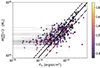 |
Fig. 4. ACT masses |

We also used the large sample of ACT DR5 clusters to estimate the scatter in mass at a given flux range. Since the X-ray data for the ACT DR5 sample were not cleaned for strong X-ray outliers (mostly due to the presence of AGN), we calculated 68% quintiles of SZ-based masses around the FX-predicted values rather than the RMS. Furthermore, taking advantage of the larger sample, we split the data into two X-ray flux bins: 3 × 10⁻¹⁴ ≤ FX < 7.5 × 10⁻¹⁴ erg s−1 cm−2 and FX ≥ 7.5 × 10⁻¹⁴ erg s−1 cm−2. Clusters with X-ray fluxes below 3 × 10⁻¹⁴ erg s−1 cm−2 were excluded to avoid too strong contribution from the photon counting noise. Two flux ranges were chosen to contain roughly the same number of objects (124/113 galaxy clusters in lower/higher flux bins). Approximately 68% of ACT masses ( ) lie within ±24% of the FX-based estimates for lower X-ray fluxes, whereas it is ±23% for higher X-ray fluxes.
The X-ray (Vikhlinin et al. 2009) and SZ (Orlowski-Scherer et al. 2021; Hilton et al. 2021) samples both cover approximately the same mass range M ≳ 1.5 × 10¹⁴ M⊙, but the SZ-based sample extends to higher redshifts. Therefore, our analysis confirms that FX remains a crude indicator of cluster masses for higher mean redshifts than the original X-ray sample of Vikhlinin et al. (2009). We note that there is no guarantee that an extrapolation to lower masses (groups of galaxies) holds, too. In particular, at lower temperatures, the X-ray emissivity depends strongly on the abundance of metals and varies non-monotonically with temperature (see, e.g., Fig. B.2 in Lyskova et al. 2023).
5. Conclusions
Our results can be summarized as follows. Using a combination of eROSITA X-ray data and SZ-based measurements of galaxy cluster masses from ACT samples, we confirmed that observed X-ray flux (rather than luminosity) in the 0.5−2 keV band can be used as a direct proxy for cluster masses at z ≳ 0.6 − 0.7 in the form
 (3)
(3)
suggested in Churazov et al. (2015) to which we have added a correction factor z0.5 to extend the applicability range. This relation is based on the extrapolation of the X-ray-based scaling relations from Vikhlinin et al. (2009) and the standard ΛCDM model. Using the sample of Orlowski-Scherer et al. (2021), which consists of clusters detected both in the MaDCoWS (Gonzalez et al. 2019) and ACT data, we obtained ηUPP ≈ 0.80 if  is used. The resulting RMS deviation of the masses predicted by the best-fitting FX − M500c relation from the ACT masses is ≈34%. The masses recalibrated to match weak lensing analysis (
 ) from Hilton et al. (2021) are related as
  . Therefore, if
  is used, ηWL = ηUPP/0.71 ≈ 1.13. These results suggest that the X-ray-based scaling relations predict masses halfway between SZ and weak lensing mass calibration.
Overall, the relation of the X-ray flux and mass can be used even without knowing the exact redshift, i.e., setting z = 1, to get a rough estimate of cluster masses (as long as it is known that z ≳ 0.6 − 0.7). It is particularly useful for a preselection of massive cluster candidates for follow-up verification.
A more consistent approach would be to write a likelihood function that accounts for observational and intrinsic scatters and biases. However, for our approximate calibration, this is not required.
Calculated as a relative root mean square error =  .
.
Acknowledgments
We are very grateful to the referee for a thorough reading of the manuscript and for the valuable comments. This work is based on observations with eROSITA telescope onboard SRG observatory. The SRG observatory was built by Roskosmos in the interests of the Russian Academy of Sciences represented by its Space Research Institute (IKI) in the framework of the Russian Federal Space Program, with the participation of the Deutsches Zentrum für Luft- und Raumfahrt (DLR). The SRG/eROSITA X-ray telescope was built by a consortium of German Institutes led by MPE, and supported by DLR. The SRG spacecraft was designed, built, launched and is operated by the Lavochkin Association and its subcontractors. The science data are downlinked via the Deep Space Network Antennae in Bear Lakes, Ussurijsk, and Baykonur, funded by Roskosmos. The eROSITA data used in this work were processed using the eSASS software system developed by the German eROSITA consortium and proprietary data reduction and analysis software developed by the Russian eROSITA Consortium. IK acknowledges support by the COMPLEX project from the European Research Council (ERC) under the European Union’s Horizon 2020 research and innovation program grant agreement ERC-2019-AdG 882679. NL acknowledges financial support from the Russian Science Foundation (grant no. 25-22-00470).
References
- Allen, S. W., Evrard, A. E., & Mantz, A. B. 2011, ARA&A, 49, 409 [Google Scholar]
- Arnaud, M., Pratt, G. W., Piffaretti, R., et al. 2010, A&A, 517, A92 [CrossRef] [EDP Sciences] [Google Scholar]
- Boggs, P., Byrd, R., Donaldson, J., & Schnabel, R. 1989, User’s Reference Guide for ODRPACK: Software for Weighted Orthogonal Distance Regression Version 1.7 (Gaithersburg: National Institute of Standards and Technology) [Google Scholar]
- Brunner, H., Boller, T., Coutinho, D., et al. 2018, SPIE Conf. Ser., 10699, 106995G [Google Scholar]
- Burenin, R. A., Bikmaev, I. F., Khamitov, I. M., et al. 2018, Astron. Lett., 44, 297 [NASA ADS] [CrossRef] [Google Scholar]
- Burenin, R. A., Bikmaev, I. F., Gilfanov, M. R., et al. 2021, Astron. Lett., 47, 443 [Google Scholar]
- Churazov, E., Vikhlinin, A., & Sunyaev, R. 2015, MNRAS, 450, 1984 [CrossRef] [Google Scholar]
- Churazov, E., Khabibullin, I., Lyskova, N., Sunyaev, R., & Bykov, A. M. 2021, A&A, 651, A41 [NASA ADS] [CrossRef] [EDP Sciences] [Google Scholar]
- Coulton, W., Madhavacheril, M. S., Duivenvoorden, A. J., et al. 2024, Phys. Rev. D, 109, 063530 [NASA ADS] [CrossRef] [Google Scholar]
- DESI Collaboration (Aghamousa, A., et al.) 2016, ArXiv e-prints [arXiv:1611.00036] [Google Scholar]
- Di Gennaro, G., Brüggen, M., Moravec, E., et al. 2025, A&A, 695, A215 [NASA ADS] [CrossRef] [EDP Sciences] [Google Scholar]
- Dolag, K., Remus, R. S., Valenzuela, L. M., et al. 2025, A&A, submitted [arXiv:2504.01061] [Google Scholar]
- Gilfanov, M., Grimm, H. J., & Sunyaev, R. 2004, MNRAS, 351, 1365 [NASA ADS] [CrossRef] [Google Scholar]
- Giodini, S., Lovisari, L., Pointecouteau, E., et al. 2013, Space Sci. Rev., 177, 247 [Google Scholar]
- Gonzalez, A. H., Gettings, D. P., Brodwin, M., et al. 2019, ApJS, 240, 33 [NASA ADS] [CrossRef] [Google Scholar]
- Hilton, M., Sifón, C., Naess, S., et al. 2021, ApJS, 253, 3 [Google Scholar]
- Jenkins, A., Frenk, C. S., White, S. D. M., et al. 2001, MNRAS, 321, 372 [Google Scholar]
- Khabibullin, I. I., Churazov, E. M., Bykov, A. M., Chugai, N. N., & Sunyaev, R. A. 2023, MNRAS, 521, 5536 [NASA ADS] [CrossRef] [Google Scholar]
- Klein, M., Mohr, J. J., & Davies, C. T. 2024, A&A, 690, A322 [NASA ADS] [CrossRef] [EDP Sciences] [Google Scholar]
- Kravtsov, A. V., & Borgani, S. 2012, ARA&A, 50, 353 [Google Scholar]
- Kravtsov, A. V., Vikhlinin, A., & Nagai, D. 2006, ApJ, 650, 128 [Google Scholar]
- Kruglov, A., Khabibullin, I., Lyskova, N., Dolag, K., & Biffi, V. 2025, JCAP, 2025, 007 [Google Scholar]
- Luo, B., Brandt, W. N., Xue, Y. Q., et al. 2017, ApJS, 228, 2 [Google Scholar]
- Lyskova, N., Churazov, E., Khabibullin, I. I., et al. 2023, MNRAS, 525, 898 [NASA ADS] [CrossRef] [Google Scholar]
- Mantz, A. B., Allen, S. W., Morris, R. G., et al. 2016, MNRAS, 463, 3582 [NASA ADS] [CrossRef] [Google Scholar]
- Mantz, A. B., Allen, S. W., Morris, R. G., & von der Linden, A. 2018, MNRAS, 473, 3072 [NASA ADS] [CrossRef] [Google Scholar]
- Massey, R., Hoekstra, H., Kitching, T., et al. 2013, MNRAS, 429, 661 [Google Scholar]
- Nagai, D. 2006, ApJ, 650, 538 [Google Scholar]
- Oguri, M., & Miyazaki, S. 2025, Proc. Japan Acad. Ser. B, 101, 129 [Google Scholar]
- Orlowski-Scherer, J., Di Mascolo, L., Bhandarkar, T., et al. 2021, A&A, 653, A135 [NASA ADS] [CrossRef] [EDP Sciences] [Google Scholar]
- Planck Collaboration III. 2013, A&A, 550, A129 [NASA ADS] [CrossRef] [EDP Sciences] [Google Scholar]
- Pratt, G. W., Croston, J. H., Arnaud, M., & Böhringer, H. 2009, A&A, 498, 361 [NASA ADS] [CrossRef] [EDP Sciences] [Google Scholar]
- Pratt, G. W., Arnaud, M., Biviano, A., et al. 2019, Space Sci. Rev., 215, 25 [Google Scholar]
- Pratt, G. W., Arnaud, M., Maughan, B. J., & Melin, J. B. 2022, A&A, 665, A24 [NASA ADS] [CrossRef] [EDP Sciences] [Google Scholar]
- Predehl, P., Andritschke, R., Arefiev, V., et al. 2021, A&A, 647, A1 [EDP Sciences] [Google Scholar]
- Sheth, R. K., Mo, H. J., & Tormen, G. 2001, MNRAS, 323, 1 [NASA ADS] [CrossRef] [Google Scholar]
- Sunyaev, R. A., & Zeldovich, Y. B. 1972, Comments Astrophys. Space Phys., 4, 173 [NASA ADS] [EDP Sciences] [Google Scholar]
- Sunyaev, R., Arefiev, V., Babyshkin, V., et al. 2021, A&A, 656, A132 [NASA ADS] [CrossRef] [EDP Sciences] [Google Scholar]
- Swetz, D. S., Ade, P. A. R., Amiri, M., et al. 2011, ApJS, 194, 41 [NASA ADS] [CrossRef] [Google Scholar]
- Tinker, J., Kravtsov, A. V., Klypin, A., et al. 2008, ApJ, 688, 709 [Google Scholar]
- Umetsu, K. 2020, A&ARv, 28, 7 [Google Scholar]
- van Breukelen, C., Clewley, L., Bonfield, D. G., et al. 2006, MNRAS, 373, L26 [NASA ADS] [Google Scholar]
- van der Burg, R. F. J., Aussel, H., Pratt, G. W., et al. 2016, A&A, 587, A23 [NASA ADS] [CrossRef] [EDP Sciences] [Google Scholar]
- Vikhlinin, A., Burenin, R. A., Ebeling, H., et al. 2009, ApJ, 692, 1033 [Google Scholar]
- Warren, M. S., Abazajian, K., Holz, D. E., & Teodoro, L. 2006, ApJ, 646, 881 [NASA ADS] [CrossRef] [Google Scholar]
Appendix A: (Weak) evolution of the FX-M500 relation with redshift
We reproduce the analysis described in Churazov et al. (2015), namely, for each cluster mass M500c and redshift, we calculate the X-ray flux FX using the scaling relations from Vikhlinin et al. (2009) and assuming that they hold at redshifts of interest. We use the cluster mass function from Tinker et al. (2008) to estimate the mass range relevant for a given redshift. Next, we convert the X-ray flux FX to the cluster mass estimate MX using Eq. 1. Figure A.1 shows the ratio between MX and the true cluster mass as a function of redshift. Only clusters with M500c > 1014 M⊙ are considered. As follows from Fig. A.1, there is a weak trend with redshift which can be accounted for to improve the tightness of the correlation between the X-ray flux and the cluster mass.
 |
Fig. A.1. Expected deviation of the X-ray-flux-based mass estimate from the true (input) mass. Triangles show the ratio of the mass predicted by eq. (1) to the true M500c value for clusters that follow adopted scaling relations from Vikhlinin et al. (2009). Solid circles show the same ratio when the factor z0.5 (as in eq. 2) is accounted for. Different colors indicate the mass range of clusters that are expected to be present above a given redshift. |
Appendix B: Biases of the simple aperture photometry
Simple aperture photometry flux estimation can suffer from biases arising from fluctuations in the number of sources comprising the unresolved Cosmic X-ray Background (CXB). In this section, we briefly evaluate the magnitude of such bias using typical parameters relevant to the eROSITA all-sky survey and assess its importance.
For estimates, we used an effective exposure time of ∼700 s and the time-averaged eROSITA background rates. The total telescope count rate is composed of three main components: the instrumental background, the diffuse sky background (dominated by the Milky Way emission), and the CXB, which can be partially resolved in individual sources. On average, these three components have comparable contributions to the 0.4-2.3 keV band used in the previous sections. In Sec. 3.2, the background contribution to the cluster region (2′ radius circle) was estimated by measuring the surface brightness in a much larger region (a ring with inner and outer radii of 6′ and 20′, respectively) and multiplying it by the solid angle of the source region. While this procedure is expected to remove the particle and diffuse backgrounds accurately, the fluctuations associated with unresolved CXB sources introduce a bias in the measured flux. The bias arises due to a small number of CXB sources that can be detected and resolved with the eROSITA sensitivity and angular resolution.
There are two flavors of this bias. The first type arises because resolving background sources in close vicinity to the target cluster (without compromising the cluster flux) is more difficult than farther away from it. For that reason, a higher flux threshold for excising CXB sources might be set in the ‘cluster’ region compared to the ‘background’. As a result, the mean surface brightness in the background region is lower than in the source region, even in the absence of a cluster, and the mean cluster flux is overestimated (after averaging over many clusters; see Table B.1). However, the probability of finding a source with the flux in the relevant range in the cluster region is small. Therefore, this bias shifts the mean but does not change the mode of the distribution.
The second type of bias stems purely from a much smaller solid angle of the ‘cluster’ region than the ‘background’ region. This means that the probability of finding a bright CXB source at a given flux level in the ‘cluster’ region is smaller than in the ‘background’ region. As a result, most of the ‘cluster’ regions will lack such sources except for a few. Therefore, even if the CXB sources are removed at the same flux level and the mean surface brightness is the same, the most probable flux value (maximum of the probability distribution function) is lower in the smaller region. This is similar to the effects of low numbers statistics considered by Gilfanov et al. (2004) in the context of calculating the total luminosity of a population of discrete sources in normal galaxies.
To illustrate the magnitude of these biases, we’ve made a simple simulation of the aperture photometry flux estimation. The particle and diffuse background levels (surface brightness) were set to typical values of the eROSITA survey. For CXB modeling, we used the source counts from the Chandra deep field (Luo et al. 2017) in the 0.5-2 keV band. With these assumptions, 106 realizations of the expected fluxes in the ‘cluster’ and ‘background’ regions were performed taking into account fluctuations in the number of CXB sources below the given detection threshold (and associated count rate in the eROSITA 0.4-2.3 keV band) to which the expectation of the particle and diffuse background rates were added.
The corresponding distributions are shown in Fig.B.1 with the solid red and blue curves, while the green and black lines show the expected distributions of the flux corrected for the background without and with the account of the photon-counting-noise, respectively. Clearly, the expected distributions of fluxes (black curves) are broad, and their maxima are shifted below zero. In principle, the simulated distributions can be used to calculate the likelihood of measured fluxes in individual observations, taking into account different exposure times and different levels of the diffuse background. However, our aim is to estimate a single parameter – a normalization of the relation that links the measured X-ray flux with the mass. For this problem, the entire sample is used, and the biases can be estimated for the entire sample of 36 objects. This significantly increases the effective solid angle of the data and should reduce the scatter and some of the biases.
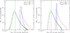 |
Fig. B.1. Expected distribution of the 0.5-2.0 keV flux in a single circular ‘source’ region (2′ radius) in the eROSITA all-sky survey (red curve) for different levels of the resolved sources in the source and background regions. The red curve corresponds to the distribution of fluxes (including diffuse and particle backgrounds) in the source region, while the blue curve shows the flux distribution in the background region (∼100 times larger solid angle) after rescaling to the area of the source region. These distributions are driven by fluctuations of CXB sources in these regions. The green curve shows the distribution of fluxes in the source region once the contribution of the background was subtracted. Finally, the black curve shows the same distribution to which photon counting noise has been added. In the left panel, only extremely bright sources are excluded with FX > 10−11 erg s−1 in the 0.5 − 2 keV band. Such sources are very rare and do not contribute much to the mean CXB background. In practice, this flux cut effectively corresponds to the case when no CXB sources are resolved. In the right panel, fainter sources (FX > 2 × 10⁻¹⁴ erg s−1) have been removed from the background region, while in the source region, only sources brighter than FX > 1 × 10⁻¹³ erg s−1 have been removed. This reduces the scatter in the estimated flux in the background region but introduces a small bias in the mean flux since a larger fraction of the mean CXB flux is resolved in the background region. |
Estimated biases in fluxes measured from the 2′ circles from simulations.
 |
Fig. B.2. Same as Fig. B.1 (right panel) after averaging over a sample of Nobj = 36 objects. Now, the distributions are much narrower, and the mode and mean of the distributions agree well and feature only a small deviation from zero. This means that while individual flux measurements have a broad and biased distribution, the mean flux of the sample has a significantly smaller bias that is largely driven by the different resolved fractions of the CXB. |
To this end, we made additional simulations that account for the effective solid angle of the entire sample rescaled as shown in Fig. B.2. In this case, the peak of the distribution becomes narrower and shifts to the positive side since the scatter associated with the fluctuations of unresolved sources is strongly reduced, but the bias associated with the different resolved fractions of the CXB background remains in place. Most importantly, the mean and the mode of the distribution now agree well. Table B.1 summarizes the biases discussed above. Our particular choice of the resolved fractions corresponds to cases shown in the right panel of Fig. B.1 (for a single object) and Fig. B.2 (for the entire sample).
Similar simulations were done for larger sample (Nobj = 364) with different CXB resolved fractions, namely FX, S > 10−11 erg s−1 and FX, B > 10−13 erg s−1 for the source and background regions, respectively. The mean and mode of the flux distribution for a single measurement and for the entire sample are shown in the last two rows of Table B.1, while the distributions themselves are shown in Fig. B.3. As expected, with these flux cuts, the flux distribution in a single measurement is broad, and its mode is shifted towards negative fluxes. In contrast, for the entire sample, the mode is much smaller and positive.
The choice of X-ray flux estimation method (forced photometry) and the simplicity of the fitting function (only the normalization is treated as a free parameter) greatly simplifies the modeling of the uncertainties associated with the removal of the astrophysical background (CXB). As already mentioned in Sec. 4.1, accurate constraints on the full scaling relation require full modeling (direct simulations) of the flux measurements, the intrinsic scatter in the cluster properties, and the biases in the selection function.
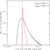 |
Fig. B.3. Simulated distribution of the background-subtracted fluxes in the 2′ circle apertures for a sample of 364 objects when CXB sources with fluxes above 10−13 erg s−1 cm−2 are resolved in the background region. The black line corresponds to a single realization, while the red line applies to the sample-averaged flux. |
All Tables
All Figures
|
Fig. 1. Sunyaev-Zel’dovich and X-ray views on the galaxy cluster ACT-CL J0105.8−1839. Left panel: Planck + ACT Compton-y map (Coulton et al. 2024). Middle panel: eROSITA 0.4−2.3 keV image. We used a ring with 6′< R < 20′ to estimate the background, and it was then subtracted from the source region (marked as a white circle). The right panel illustrates the source removal procedure. |
| In the text | |
|
Fig. 2. ACT cluster masses |
| In the text | |
|
Fig. 3. ACT masses |
| In the text | |
|
Fig. 4. ACT masses |
| In the text | |
|
Fig. A.1. Expected deviation of the X-ray-flux-based mass estimate from the true (input) mass. Triangles show the ratio of the mass predicted by eq. (1) to the true M500c value for clusters that follow adopted scaling relations from Vikhlinin et al. (2009). Solid circles show the same ratio when the factor z0.5 (as in eq. 2) is accounted for. Different colors indicate the mass range of clusters that are expected to be present above a given redshift. |
| In the text | |
|
Fig. B.1. Expected distribution of the 0.5-2.0 keV flux in a single circular ‘source’ region (2′ radius) in the eROSITA all-sky survey (red curve) for different levels of the resolved sources in the source and background regions. The red curve corresponds to the distribution of fluxes (including diffuse and particle backgrounds) in the source region, while the blue curve shows the flux distribution in the background region (∼100 times larger solid angle) after rescaling to the area of the source region. These distributions are driven by fluctuations of CXB sources in these regions. The green curve shows the distribution of fluxes in the source region once the contribution of the background was subtracted. Finally, the black curve shows the same distribution to which photon counting noise has been added. In the left panel, only extremely bright sources are excluded with FX > 10−11 erg s−1 in the 0.5 − 2 keV band. Such sources are very rare and do not contribute much to the mean CXB background. In practice, this flux cut effectively corresponds to the case when no CXB sources are resolved. In the right panel, fainter sources (FX > 2 × 10⁻¹⁴ erg s−1) have been removed from the background region, while in the source region, only sources brighter than FX > 1 × 10⁻¹³ erg s−1 have been removed. This reduces the scatter in the estimated flux in the background region but introduces a small bias in the mean flux since a larger fraction of the mean CXB flux is resolved in the background region. |
| In the text | |
|
Fig. B.2. Same as Fig. B.1 (right panel) after averaging over a sample of Nobj = 36 objects. Now, the distributions are much narrower, and the mode and mean of the distributions agree well and feature only a small deviation from zero. This means that while individual flux measurements have a broad and biased distribution, the mean flux of the sample has a significantly smaller bias that is largely driven by the different resolved fractions of the CXB. |
| In the text | |
|
Fig. B.3. Simulated distribution of the background-subtracted fluxes in the 2′ circle apertures for a sample of 364 objects when CXB sources with fluxes above 10−13 erg s−1 cm−2 are resolved in the background region. The black line corresponds to a single realization, while the red line applies to the sample-averaged flux. |
| In the text | |
Current usage metrics show cumulative count of Article Views (full-text article views including HTML views, PDF and ePub downloads, according to the available data) and Abstracts Views on Vision4Press platform.
Data correspond to usage on the plateform after 2015. The current usage metrics is available 48-96 hours after online publication and is updated daily on week days.
Initial download of the metrics may take a while.