| Issue |
A&A
Volume 702, October 2025
|
|
|---|---|---|
| Article Number | A225 | |
| Number of page(s) | 13 | |
| Section | Stellar structure and evolution | |
| DOI | https://doi.org/10.1051/0004-6361/202556452 | |
| Published online | 24 October 2025 | |
Characterising the short-orbital period X-ray transient Swift J1910.2–0546
1
European Southern Observatory, Casilla 19001, Vitacura, Santiago, Chile
2
Instituto de Astrofísica de Canarias, E-38205 La Laguna, Tenerife, Spain
3
Departamento de Astrofísica, Universidad de La Laguna, E-38206 La Laguna, Tenerife, Spain
4
Department of Astrophysics/IMAPP, Radboud University Nijmegen, PO Box 9010 Nijmegen 6500 GL, The Netherlands
5
SRON, Netherlands Institute for Space Research, Niels Bohrweg 4, Leiden 2333 CA, The Netherlands
6
Max Planck Institute for Astronomy, Königstuhl 17 69117 Heidelberg, Germany
7
Astronomy, Engineering, and Physics Department, Fresno City College, 1101 East University Ave., Fresno, CA 93741, USA
8
Instituto de Alta Investigación, Universidad de Tarapacá, Casilla 7D, Arica, Chile
9
School of Physics & Astronomy, University of Southampton, Southampton SO17 1BJ, UK
10
Astrophysics, Department of Physics, University of Oxford, Keble Road, Oxford OX1 3RH, UK
11
Department of Physics, 2345 San Ramon Ave., M/S MH37, California State University, Fresno, CA 93740, USA
12
Gran Telescopio Canarias, Cuesta de San José s/n, Breña Baja 38712, Santa Cruz de Tenerife, Spain
13
Center for Astro, Particle and Planetary Physics, New York University Abu Dhabi, PO Box 129188 Abu Dhabi, UAE
⋆ Corresponding author: This email address is being protected from spambots. You need JavaScript enabled to view it.
Received:
16
July
2025
Accepted:
19
August
2025
Abstract
Context.Swift J1910.2–0546 (=MAXI J1910−057) is a Galactic X-ray transient discovered during a bright outburst in 2012. Its X-ray spectral and timing properties point to a black-hole accretor, yet the orbital period remains uncertain, and no reliable dynamical constraints on the binary parameters are available. The 2012 event, extensively monitored at X-ray and optical wavelengths, offers a rare opportunity to investigate the structure and dynamics of the system and to constrain its fundamental properties.
Aims. We use time-series optical photometry and spectroscopy, obtained during outburst and quiescence, to estimate the orbital period, characterise the donor star, determine the interstellar extinction, distance, and system geometry, and constrain the component masses.
Methods. Multi-site r-band and clear-filter light curves and WHT/ACAM spectra from the 2012 outburst were combined with time-series spectroscopy from GTC/OSIRIS and VLT/FORS2 in quiescence. Period searches were conducted using generalised Lomb–Scargle, phase-dispersion minimisation, and analysis-of-variance algorithms. We used diffuse interstellar bands to constrain E(B − V), while empirical correlations involving Hα yielded estimates of K2, q, and i.
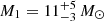
Results. We detected a coherent, double-humped modulation with a period of 0.0941 ± 0.0007 d (2.26 ± 0.02 h) during the outburst. Its morphology is consistent with an early superhump, suggesting that the true orbital period may be slightly shorter than 4.52 h. The Hα radial velocity curves do not yield a definitive orbital period. In quiescence, TiO bands indicate an M3−M3.5 donor contributing ≃70% of the red continuum. Diffuse interstellar bands give E(B − V) = 0.60 ± 0.05 and NH = (3.9 ± 1.3)×1021 cm−2, placing the system at a distance of 2.8−4.0 kpc. The Hα line width in quiescence (FWHM0 = 990 ± 45 km s−1), via a FWHM–K2 calibration, provides an estimate of K2, while its double-peaked profile gives q and the orbital inclination. The latter appears much higher than estimates from X-ray studies. Adopting the resulting K2 = 230 ± 17 km s−1 and q = 0.032 ± 0.010, along with two orbital period scenarios (2.25 and 4.50 h), Monte Carlo sampling returns a compact object mass of M1 = 8 − 11 M⊙ and an inclination of i = 13° −18° for plausible donor masses (M2 = 0.25 − 0.35 M⊙). Overall, we favour an orbital period of 4.5 h.
Conclusions.Swift J1910.2–0546 may be a short-period, low-inclination black hole X-ray transient, although the possibility of it being a neutron star accretor cannot be completely ruled out. Subsequent phase-resolved spectroscopy and photometry during quiescence are needed to better determine its fundamental parameters.
Key words: accretion, accretion disks / binaries: close / stars: black holes / stars: individual: Swift J1910.2–0546 / X-rays: binaries
© The Authors 2025
 Open Access article, published by EDP Sciences, under the terms of the Creative Commons Attribution License (https://creativecommons.org/licenses/by/4.0), which permits unrestricted use, distribution, and reproduction in any medium, provided the original work is properly cited.
This article is published in open access under the Subscribe to Open model. This email address is being protected from spambots. You need JavaScript enabled to view it. to support open access publication.
1. Introduction
Low-mass X-ray binaries (LMXBs) are systems in which either a stellar-mass black hole (BH) or a neutron star accretes material from a low-mass companion star through Roche-lobe overflow. Among them, X-ray transient systems undergo sporadic outbursts driven by thermal-viscous instabilities in the accretion disc Lasota 2001, resulting in multi-wavelength brightness increases.
During outburst, distinct accretion-related phenomena are observed in X-rays (e.g. Done et al. 2007; Belloni 2010), while jets are observed in the radio band (e.g. Fender et al. 2004). The optical spectrum is typically dominated by emission lines formed in the outer disc atmosphere, which are sometimes observed to show signatures of accretion disc winds (e.g. Muñoz-Darias et al. 2019). These are also detected in X-rays in highly inclined systems (e.g. Ponti et al. 2012). As the system fades exponentially back to quiescence, rebrightening events may occur (e.g. Truss et al. 2002; Zurita et al. 2002; Jiménez-Ibarra et al. 2019; Zhang et al. 2019).
Thus far, BHs in Galactic LMXBs have been predominantly found in transient systems. However, despite decades of study, only ≈20 out of 72 BH candidates have been dynamically confirmed (see BlackCAT1; Corral-Santana et al. 2016). This is due to the difficulty of performing dynamical studies during quiescence, where the donor star dominates the optical light Charles & Coe 2006. Moreover, constraining the BH mass requires measuring the orbital period and radial velocity amplitude of the donor, as well as additional parameters, such as the binary mass ratio and system inclination.
Swift J1910.2–0546 (hereafter J1910), also known as MAXI J1910−057, is a Galactic X-ray transient first detected on 30 May 2012 by the Burst Alert Telescope (BAT) on board the Neil Gehrels Swift Observatory, and independently by the Monitor of All-sky X-ray Image/Gas Slit Camera (MAXI/GSC) Krimm et al. 2012; Usui et al. 2012. Kimura et al. 2012 analysed a MAXI/GSC spectrum collected between 12 and 14 June 2012 and found that it can be adequately modelled by a disc blackbody. The thermal nature of the emission is broadly consistent with the soft spectral state seen in other black hole candidates. An optical/near-infrared counterpart was identified shortly after the onset of the outburst at RA, Dec (ICRS) = 19:10:22.79, −05:47:55.9 (Rau et al. 2012; Cenko & Ofek 2012, see Fig. 1).
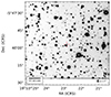 |
Fig. 1. VLT/FORS2 I-band acquisition image obtained during quiescence. J1910 is marked with a red cross at the centre of the 1.2′ field. North is up, east is to the left. |
Early optical spectroscopy taken on 18 June 2012 revealed an almost featureless blue continuum, lacking Balmer or He I lines, but displaying a broad He IIλ4686 emission line Charles et al. 2012. Subsequent spectroscopy, revisited here (see Sect. 2.1 for details), showed a weak He IIλ4686 emission line, broad Hβ and Hγ absorptions, and a wide Hα absorption trough with a weak emission component as reported in Casares et al. 2012, who tentatively constrained the orbital period to be > 6.2 h. However, Lloyd et al. 2012 had earlier reported a putative modulation at 2.25−2.47 h, which, if confirmed, would make J1910 the shortest orbital period BH X-ray binary known to date.
By early 2013, the system was considered to be in quiescence Nakahira et al. 2014; Saikia et al. 2023a. In July 2015, López et al. 2019 obtained optical/near-infrared photometry, reporting AB magnitudes of r = 23.46 ± 0.07, i = 22.18 ± 0.04, and Ks = 20.43 ± 0.11. However, Saikia et al. 2023a later reported values that were approximately one mag brighter around the same time (see their Fig. 8), attributing this discrepancy to photometry contamination from nearby field stars or to intrinsic accretion variability within the system.
J1910 remained in quiescence for about ten years, showing occasional reflares and rebrightenings during that period (see Saikia et al. 2023a, for a comprehensive study) until 8 Feb. 2022, when Tominaga et al. 2022 reported a new outburst detected by MAXI. This event was also observed in radio Williams et al. 2022 and optical wavelengths Hosokawa et al. 2022; Kong 2022. By late Mar. 2022, the system was reported to have returned to quiescence Saikia et al. 2022.
In this paper, we present the analysis of time-series optical photometry and spectroscopy of J1910 during its 2012 outburst and subsequent decline, along with additional spectroscopy obtained in 2016 when the system was in quiescence. Section 2 details the observations and data reduction processes. Section 3 presents the results, including an estimate of the orbital period, spectral type of the donor star, estimation of the distance, and constraints on the binary parameters. Section 4 discusses the implications of our findings. Section 5 contains our conclusions.
2. Observations and data reduction
2.1. Optical photometry and spectroscopy during outburst
The time-series photometry of J1910 in the r-band was obtained in June 2012 (see Table 1 for a detailed log of the observations) using the Wide Field Camera (WFC) mounted on the 2.5-m Isaac Newton Telescope (INT) at the Roque de los Muchachos Observatory (La Palma). The WFC is a prime-focus mosaic of four 2048 × 4100 pixel EEV42 CCDs, offering a field of view of approximately 34′×34′. In this study, only CCD #4 was used for imaging with an exposure time of 5 s. We conducted variable-aperture photometry of J1910 relative to the comparison star Gaia DR3 4206052097085749760 (r = 15.311 ± 0.001 in Pan-STARRS1; Chambers et al. 2016) using the HiPERCAM reduction software2.
Photometric data obtained in 2012.
We extended the time baseline by adding time-series r-band imaging with the Small and Moderate Aperture Research Telescope System (SMARTS) Consortium 0.9-m telescope on Cerro Tololo (Chile), conducted on the night of 4 June 20123, as reported in Britt et al. 2012. The 2048 × 2048 pixel Tek2K CCD detector was used with exposure times of 120 s. We performed relative photometry on the reduced images using the HiPERCAM pipeline and the same comparison star as that used for the WFC photometry.
In Sect. 3.2, we also reanalyse some of the 2012 photometric data sets originally presented in the Master’s thesis of co-author Trelawny Trelawny 2013. Specifically, we focus on the data collected during 27, 28 June and 10 and 20 July 2012, which exhibited the clearest variability. The images were obtained with the DFM Engineering 0.41-m f/8 telescope at Fresno State’s facility of the Sierra Remote Observatories (SRO), equipped with a 4008 × 2672 pixel Santa Barbara Instruments Group STL–11000M CCD camera binned 3 × 3, and an Astrodon clear filter. The Clear filter had a nearly uniform, 95−98% transparency to light with wavelengths of 3750−12 000 Å. Each frame had an exposure time of 120 s. All data were processed using the AIP4WIN 2.1.8 software Berry & Burnell 2005.
We also obtained time-series optical spectroscopy of J1910 on 28 July and 16 August 2012, a few weeks after the beginning of the outburst, using the Auxiliary-port CAMera (ACAM) mounted on the 4.2-m William Herschel Telescope (WHT) on La Palma. We obtained thirty-five 300-s (signal-to-noise ratio, S/N, of approximately 40 − 60 per pixel), and ten 600-s (S/N ≈ 40 − 75 per pixel) spectra, respectively, using a 0.5″ slit width. The 400-line/mm−1 transmission volume phase holographic grating (λλ3950−9400) was used, with a resolving power of λ/Δλ ≃ 900. The full width at half maximum (FWHM) of the night-sky [O I] emission line at 5577.338 Å was measured to be ≃6.3 Å (≃290 km s−1), taken as Δλ. The average seeing was approximately 0.7″ on both nights, so the spectra were slit-limited. The data were de-biased, flat-fielded and wavelength-calibrated using standard procedures, and cover the range λλ6000−8000. The rms scatter of the pixel-to-wavelength calibration fit was ≃0.1 Å.
Fig. 2 shows the evolution of the 2012 outburst in X-rays and in three of the optical bands of Saikia et al. 2023a. In the figure, we mark the dates on which the WHT/ACAM time-resolved spectroscopy and the photometry mentioned above and listed in Table 1 were obtained.
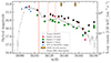 |
Fig. 2. Evolution of the 2012 outburst. X-ray data are shown as a grey line, while the R-, V-, and i′-band magnitudes published by Saikia et al. 2023a are represented by red diamonds, green squares, and black circles, respectively. Time-series photometry obtained with the SMARTS 0.9-m and INT/WFC in the r-band is marked with blue triangles, whereas the time of the WHT/ACAM spectra are indicated by orange arrows. Clear-filter photometry from Fresno SRO is marked by vertical red lines. |
2.2. Optical spectroscopy and photometry during quiescence
Five 1800-s spectra were obtained on 1 August 2016, approximately 1500 days after discovery, when J1910 was about eight magnitudes fainter than at the peak of the outburst.
For these observations, we used the Optical System for Imaging and low-Intermediate-Resolution Integrated Spectroscopy (OSIRIS) instrument Cepa et al. 2003 mounted on the 10.4-m Gran Telescopio Canarias (GTC) at the Roque de los Muchachos Observatory. The data were taken using the R1000R grism (λλ5200−10 200, mean reciprocal dispersion of 2.6 Å pixel−1) with a 0.8″ slit width, providing a resolution of approximately 7.1 Å, and a S/N per pixel of ≈10 in the continuum close to Hα. The rms scatter of the pixel-to-wavelength calibration fit is 0.11 Å. The average seeing conditions on that night were around 1″. The reduction process for these spectra was similar to that used for the outburst WHT/ACAM data. To correct for the instrumental response, we used the spectrophotometric standard Feige 66 Oke 1990.
We note that the OSIRIS i-band acquisition images show that J1910’s PSF is contaminated by two much brighter stars located just to the south. Although these sources are well resolved in Fig. 1, the relatively poor seeing conditions during the OSIRIS observations allowed flux from the nearby stars to enter the slit. This resulted in a dilution of the target spectrum, which may have contributed to the differences discussed in Section 3.3.
Further optical spectroscopy was conducted using the Very Large Telescope (VLT) located at Cerro Paranal, Chile, while J1910 was in quiescence. The FORS2 spectrograph was configured with the 600RI grism and a 1″ slit width, yielding a useful spectral range of 5330−8385 Å. The average seeing during the observations, as measured by collapsing the 2D spectra along the dispersion axis in the vicinity of Hα, ranged from 0.35″ to 0.94″, resulting in a spectral resolution of 3.3−5.0 Å, corresponding to velocity resolutions of approximately 160−240 km s−1 at 6300 Å.
The spectra were acquired with the MIT/LL mosaic detector, binned 2 × 2. The observations took place between 30 April and 5 September 2016, when a total of 15 spectra were obtained. Each exposure had a duration of 1270 s, and the S/N per pixel of the extracted spectra in the vicinity of Hα is in the range ≈2 − 8. As mentioned earlier, the average seeing during these exposures ranged from 0.35″ to 0.94″, providing sufficient spatial resolution to distinguish J1910 from the nearby brighter star located 1.3″ south of the target (see Fig. 1). As this star was simultaneously included on the slit, we used its spectrum to correct for telluric absorptions after masking out any stellar features. We corrected the FORS2 spectra of J1910 for instrumental response using an ESO archive spectrum of the standard star LTT 7379 Hamuy et al. 1992, 1994, obtained on the night of 3 September 2016.
The acquisition images taken prior to each FORS2 spectrum were obtained in the I-band using the I_BESS+77 filter, with an exposure time of 120 s. These images were processed using point spread function (PSF) photometry with DAOPHOT II/ALLSTARStetson 1987. To calibrate our I-band photometry, we cross-matched the resulting source catalogue with Pan-STARRS1 (AB magnitudes; Chambers et al. 2016) and converted these magnitudes to the Johnson-Cousins I-band using the transformation equations provided in Table 6 of Tonry et al. 2012. Approximately 50 stellar-like sources per image (defined by a sharpness value ≤0.1) with relatively low PSF photometric uncertainties (≤0.05 mag) were used to derive the individual zero-points. The resulting magnitudes are listed in Table 2.
We also performed PSF photometry on the average OSIRIS i-band acquisition image using DAOPHOT II/ALLSTAR, and estimated the zero-point by following a procedure similar to that used for the FORS2 acquisition images. With a total of 37 stars in common with Pan-STARRS1 in our catalogue, we derived i = 22.18 ± 0.03 for J1910, identical to that reported in López et al. 2019. A comparison with the FORS2 PSF catalogues indicates a systematic difference of approximately 0.54 mag, which accounts for the different photometric systems. This would correspond to an OSIRIS magnitude of roughly I ≃ 21.65, consistent with the values in Table 2.
Log of 2016 VLT/FORS2 spectroscopic observations of J1910 during quiescence.
3. Results
3.1. The outburst spectrum
During the 2012 outburst, the ACAM spectra of J1910 exhibit a range of spectral features, as shown in Fig. 3. The Balmer series is detected, from Hα to Hδ, with the lines displaying both emission and broader absorption components. Hα is the strongest of the emission lines, characterised by a narrow, single-peaked profile. Weaker emission lines of He Iλ5876 and possibly λ6678 are also present, while the He IIλ4686 emission line is clearly detected.
We measured the intrinsic Hα FWHM (FWHM0, corrected for the instrumental profile) by fitting Gaussian profiles, obtaining values of 540 ± 20 and 570 ± 40 km s−1 for the first and second night, respectively. The corresponding equivalent widths (EW) are 2.30 ± 0.03 and 1.83 ± 0.04 Å. Although there were no significant differences in the average spectra of both nights (see Fig. 3), we chose not to combine them, as J1910 was in a different X-ray state on each occasion, with the soft X-ray flux rapidly decreasing between the two epochs (see Fig. 2; see also Nakahira et al. 2012, 2014). The measured FWHM values are consistent with those observed in low-inclination systems in outburst, such as MAXI J1836−194 (≈270 km s−1; Russell et al. 2014).
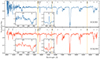 |
Fig. 3. Average spectra of J1910 during outburst from the first (upper; blue) and second (lower; red) nights, obtained with ACAM after continuum normalisation. The Balmer series down to Hδ is visible, exhibiting both emission and absorption components. Zoomed-in regions show the areas around Hα and Hβ. He I and He II lines are also present and identified in the spectra, along with several diffuse interstellar bands marked with orange bars. |
Interstellar absorption features were also present, the most prominent being the unresolved Na I doublet adjacent to He Iλ5876. Several diffuse interstellar bands (DIBs) were detected as well and three of them (at 5780, 5797, and 6614 Å) were later used to estimate the colour excess (Sect. 3.4).
3.2. Light curve period search
We conducted a search for periodicities in the SMARTS r-band light curve obtained on 4 June 2012, about six days before the peak of the 2−20 keV X-ray light curve (see Fig. 2). We also searched for the WFC r-band light curves from 9, 10, and 11 June 2012, during the outburst phase (corresponding to the first four light curves in Fig. 4). This analysis specifically targets epochs where the system maintained an almost constant average flux level, with a nightly time baseline exceeding 3.5 hours.
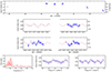 |
Fig. 4. Top panel: r-band light curves from SMARTS 0.9-m and INT/WFC, expressed as flux ratios and magnitudes, relative to the comparison star. Middle panels: SMARTS light curve (top left) and INT/WFC light curves from the first three nights when J1910 maintained an almost constant flux level, after subtracting the nightly averages. The red dashed curve represents the best-fit sine wave with a period corresponding to the highest peak in the periodogram shown below. Bottom left panel: GLS periodogram of the four r-band light curves displayed in the middle panels (4, 9, 10, and 11 Jun. 2012). The highest peak corresponds to a period of 0.0941 d ( = 2.26 h). Bottom middle and right panels: The four light curves folded on this period and twice that value. The pale blue points represent the unbinned data, while the purple points are binned data across 40 phase intervals. The zero phase corresponds to the HJD of the first data point and a full cycle is repeated for continuity. |
Prior to the period search, we subtracted the nightly mean relative flux values. The resulting light curves, depicted in the middle panels of Fig. 4, underwent a generalised Lomb-Scargle analysis (GLS; Zechmeister & Kürster 2009), based on a fitting function that includes a constant term and a sine wave. We employed the GLS class from PYASTRONOMY4Czesla et al. 2019 for this analysis.
We first estimated the period uncertainty using a bootstrap approach with flux perturbation. For each of 100 000 iterations, the light curve was resampled with replacement and the fluxes were randomly perturbed within their uncertainties. A GLS periodogram was computed for each realisation, and the frequency of the highest peak was recorded. The resulting distribution of peak periods was fitted with a Gaussian over a restricted interval around the dominant peak, and the mean and standard deviation were adopted as the representative period and its 1σ uncertainty. While this bootstrap-based method provides a formal estimate of the period uncertainty, we find that it can yield unrealistically small values, typically of the order of a few 10−5 d. This level of precision is inconsistent with the width of the corresponding peaks in the periodograms, which often have full widths at half maximum of FWHM ∼ 0.1 d−1. This discrepancy indicates that the bootstrap approach underestimates the true uncertainty, likely because it captures only the statistical noise in the flux values. Thus, it does not include broader effects such as spectral leakage, aliasing, or the finite frequency resolution imposed by the time baseline. To obtain a more realistic estimate, we adopted as the period uncertainty the value implied by the FWHM of the main periodogram peak, converted to the period domain.
The bottom-left panel of Fig. 4 illustrates the resulting periodogram, which yields a preferred period of 0.0941(5) d ( = 2.26(1) h; the numbers in parentheses indicate the 1σ uncertainties in the last digits). Consistent results were obtained using alternative period search methods, including phase dispersion minimisation (PDM; Stellingwerf 1978) and analysis of variance (AOV; Schwarzenberg-Czerny 1996) techniques. The bottom-middle panel shows the r-band light curves from 4, 9, 10, and 11 June 2012, folded on the detected period (pale blue dots) and binned into 40 phase intervals (purple dots). This period is close to the values of 0.09353(2) d ( = 2.2447(5) h) and 0.09245(2) d ( = 2.2188(5) h) reported by Lloyd et al. 2012, which were derived from observations conducted between 14 June and 7 Jul 2012, with coverage of 2 to 7 hours per night.
We repeated the analysis using all the light curves, subtracting the nightly linear trends of the last two to account for the overall brightness decline. The highest peak in the GLS periodogram also corresponds to a period of 2.26(1) h.
We also subjected the June and July 2012 Fresno SRO light curves to a GLS period search (illustrated in Fig. 5), similar to the analysis performed on the combined SMARTS and WFC time-series data. The preferred period is 0.0948(1) d ( = 2.275(3) h). In this case, the AOV periodogram shows the strongest peak near 0.19 d, while the PDM periodogram displays a corresponding minimum at the same period; both also contain signal near half that value at approximately 0.095 d.
 |
Fig. 5. Top panel: Clear-filter light curves from Fresno SRO on 27, 28 June, and 10, 20 July 2012. Middle panels: Zoomed-in view of the four light curves. The red dashed curve represents the best-fit sine wave with a period corresponding to the highest peak in the periodogram shown below. Bottom left panel: GLS periodogram of the four clear-filter light curves shown in the middle panels after subtraction of nightly averages. The highest peak corresponds to a period of 0.0948 d (2.275 h). Bottom middle and right panels: The four light curves folded on this period and twice that value. The pale blue points represent the unbinned data, while the purple points are binned data across 40 phase intervals. Zero phase is the HJD of the first data point. |
Finally, our GLS period analysis of the combined light curve set (SMARTS, WFC, and Fresno SRO) yielded a best period of 0.0941(7) d ( = 2.26(2) h). A summary of the light curve period search results is provided in Table 3.
Results of the light curve period search.
Saikia et al. 2023b tentatively suggested an orbital period in the range 2.25−2.47 h based on their analysis of B-band photometry obtained on 16 and 19 July 2012. Upon re-examining their data, we find that only the observations from the first night (represented by red circles in their Fig. 4) may exhibit a distinct modulation. Our sine-wave fit to these data yields a periodicity of 0.103(1) d ( = 2.47(2) h). However, the short duration and sparse sampling of the original observations limit the accuracy of any period determination, especially in comparison to the more extensive dataset presented here.
3.3. Hα emission radial velocity curves in quiescence from OSIRIS and FORS2
Figure 6 (top) shows the average of the five OSIRIS spectra of J1910 obtained on 1 August 2016, approximately one year after the data published by López et al. 2019. Notably, the OSIRIS spectrum exhibits features around 7000 Å that resemble those of mid-M dwarfs, although these are diluted due to significant slit contamination from the two much brighter nearby stars, caused by seeing conditions exceeding 1″. This is confirmed by the detection of an M-dwarf donor in the FORS2 quiescent spectrum.
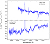 |
Fig. 6. Top panel: Average GTC/OSIRIS spectrum of J1910 during quiescence. The bluer part has been trimmed due to unreliable correction for the instrumental response. Although veiled by slit contamination from the two nearby stars (see Fig. 1), caused by seeing ≳1″, TiO absorption bands characteristic of M-stars are present in the 6800−7200 Å wavelength range. Bottom panel: The detection of an M-star donor is confirmed by the telluric-corrected, average VLT/FORS2 spectrum also obtained during quiescence. Both average spectra were dereddened using E(B − V) = 0.6 (see Sect. 3.4), and the FORS2 spectrum was smoothed with a Savitzky-Golay filter, employing a window length of nine data points and a third-order fitting polynomial for illustrative purposes. |
The S/N of the individual OSIRIS spectra is sufficient for a radial velocity analysis based solely on the Hα emission line from the accretion disc. Prior to measuring the velocities, we re-binned the spectra to a uniform velocity scale in a heliocentric frame and normalised them using a spline fit to the continuum using MOLLY5. We determined the radial velocity of the Hα emission line for each spectrum by cross-correlating its profile with a double-Gaussian template, following the method described by Schneider & Young 1980.
We tested double-Gaussian separations ranging from 1300 to 2300 km s−1 for a Gaussian FWHM of 300 km s−1, and fitted a sine function to each resulting radial velocity curve to analyse how the best-fit period varied with separation. This is illustrated in the top panel of Fig. 7, which shows the best-fit period increasing from 0.066 ± 0.05 to 0.13 ± 0.05 d. Beyond a separation of 2000 km s−1, the two Gaussians of the cross-correlation template begin to enter the continuum.
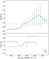 |
Fig. 7. Top panel: Best sine-fit periods derived from the radial velocity curves of the Hα emission line in the OSIRIS spectra, as a function of the double-Gaussian separation used in the velocity extraction. The shaded horizontal band indicates the periods derived from the light curves. Error bars represent 1σ uncertainties. Bottom panel: Periods corresponding to the highest peaks in the GLS (blue circles) and AOV (orange squares) periodograms derived from the quiescent FORS2 Hα radial velocity curves, as a function of the Gaussian separation used to extract the velocities. The period search was restricted to the range 0.068−0.25 d. The lower shaded horizontal band marks the periods observed in the photometric light curves, while the upper band corresponds to twice these values. |
We repeated the analysis using Gaussian FWHMs ranging from 250 to 400 km s−1 in steps of 50 km s−1 and found no significant differences. Given the limited number of radial velocity measurements (five data points) spanning only ≈0.095 d, the period determination is severely constrained. Although sine fitting can in principle be applied, the small number of observations provides little redundancy and renders the solution highly sensitive to noise and outliers. Furthermore, the short time baseline leads to strong degeneracies between period and phase, increasing the risk of aliasing and spurious fits. As such, reliable period recovery from the OSIRIS spectra alone is not feasible.
We followed the same procedure for the quiescent FORS2 spectra. We subsequently computed GLS and AOV periodograms from the resulting radial velocity curves scanning periods between 0.068 and 0.25 d. The highest peak periods vary with Gaussian separation and have approximate values of 0.14, 0.16, and 0.19 d (Fig. 7, bottom panel). The latter happens to be about twice the typical periodicity observed in the light curves; however, we deem the time sampling of our Hα radial velocity curve during quiescence too scarce to conduct a reliable period search. In fact, from the minimum time separation between two consecutive samples in our data, Δt, the pseudo-Nyquist period is 2 × min(Δt)≈0.068 d. For non-uniform sampling, the effects of aliasing and windowing stand in the way of a reliable recovery of periods close to this value VanderPlas 2018, and candidates shorter than about (4 − 5)×min(Δt)≈0.14 − 0.17 d should not be trusted. This places the observed highest-peak periods at the edge of reliable detectability.
Comparison of the average FWHM0 and EW of the Hα line measured in the spectra of J1910 taken during outburst and quiescence.
3.4. Constraints on reddening from DIBs
In the absence of a Gaia DR3 Gaia Collaboration 2023 counterpart and thus no parallax for J1910, we estimated the reddening using diffuse DIBs. We excluded those affected by strong blending or poorly defined continua and instead focussed on 5780, 6614, and 8621 Å. The reddening was derived from the measured EWs of these DIBs using the empirical relations from Munari et al. 2008 and Lan et al. 2015, and Krełowski et al. 2019 for the 5780-Å band. The results are presented in Table 5.
EW and E(B − V) obtained for selected interstellar features.
The values obtained from the interstellar Na I doublet and the 8621-Å band provide lower bounds and are consistent with the reddening inferred from the 6614-Å DIB, as is the value from the 5780-Å band. Additionally, the DIBs at 5780 and 6614 Å can be used to estimate the hydrogen column density (NH) following the empirical relations of Lan et al. 2015, serving as a consistency check for our reddening measurements. We find NH = (3.9 ± 1.3)×1021 cm−2, in agreement with values of NH ≈ (3.5 − 4.0)×1021 cm−2 derived from X-ray spectroscopy during the outburst by Degenaar et al. 2014 and Nakahira et al. 2014. Using the relation from Güver & Özel 2009, NH = 2.21 × 10²¹ AV, and adopting RV = 3.1, we find these values correspond to E(B − V)≈0.51 − 0.58, in line with our results. Finally, we adopted E(B − V) = 0.6 for J1910.
The adopted reddening value corresponds to E(g − r) values of 0.68 and 0.61 when using the Bayestar19-recommended conversion, E(B − V) = 0.884 E(g − r), or E(B − V) = 0.981 E(g − r) Schlafly & Finkbeiner 2011, respectively. However, the Bayestar19 dust map along the line of sight to J1910 saturates at E(g − r)≈0.58, which may reflect limitations in the 3D dust map’s ability to trace dense or complex sight lines. This is particularly true in regions of high extinction or low Galactic latitude, where dust maps are known to saturate or under-predict reddening due to limited background stars (see e.g. Green et al. 2019).
3.5. Detection of the donor star in quiescence: spectral type and distance
We present the dereddened average spectrum of J1910 computed from the VLT/FORS2 data obtained during quiescence in the bottom panel of Fig. 6. For the averaging process, we included only the spectra where the donor star is more prominently detected (spectra 8, 12, 13, and 14 in Table 2).
In the wavelength range sampled by our FORS2 data, the spectrum of J1910 in quiescence is dominated by the flux from an M-type star and broad Hα emission (FWHM0 ≈ 1000 km s−1; Table 4). The observed FWHM0 of Hα during quiescence is too large to originate from the companion star, whose Hα emission typically exhibits FWHM values of only a few hundred km s−1 (e.g. Ratti et al. 2012 for a neutron star X-ray binary and Rodríguez-Gil et al. 2015, 2020 for nova-like cataclysmic variables in the low state). The large width and double-peaked morphology of the line are instead consistent with an accretion disc origin (see Fig. 8).
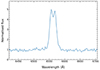 |
Fig. 8. Average of the 15 FORS2 spectra obtained during quiescence. The profile of the Hα emission line is double-peaked. |
The TiO band head at 7165 Å is distinctly evident, while that at 7665 Å is also prominently observed. Young & Schneider 1981 and Wade & Horne 1988 demonstrated that the TiO band ratio, 7165 Å/7665 Å, is sensitive to spectral type. Following the latter authors, we fitted a first-order polynomial to the continuum over the wavelength ranges λλ7450−7550 and λλ8130−8170 and calculated the flux deficits using the equations:
and
where fλ is the flux density of the spectrum and cλ represents the flux density of the linear fit to the selected continuum regions. We computed both the ratio of these deficits to the continuum flux at 7500 Å and the deficit ratio for J1910 and selected flux-calibrated and dereddened M-dwarf spectra from the X-shooter Spectral Library (XSL) DR3 Verro et al. 2022, spanning the spectral types M0 to M56, after degrading to match the FORS2 resolution. For J1910, we obtained a TiO deficit ratio of 1.76 ± 0.17 and a fractional depth of the TiO λ7665 band of 0.17 ± 0.01, with the 1σ uncertainties derived from 10 000 Monte Carlo simulations. The results are illustrated in Fig. 9, which also includes results from Marsh 1990. The spectral types of the observed M-type stars reported in that study were adopted from Boeshaar 1976, with additional comparison points included from Wade & Horne 1988. We revised the Boeshaar spectral types adopted by Wade & Horne 1988 using updated and consistent classifications retrieved from the literature via SIMBAD Wenger et al. 2000: Gl 328 (M0), Gl 381 (M2.5), Gl 273 (M3.5), Gl 299 (M4.5), and Gl 285 (M4.5). We were unable to revise the spectral types of the M-type stars observed by Marsh 1990 because their names were not reported and the observing logs are not available.
 |
Fig. 9. Fractional depth of the TiO λ7665 band as a function of the TiO band deficit ratio for J1910 and comparison M-type stars. Blue dots indicate X-shooter Library M dwarfs, while grey triangles correspond to those used by Marsh 1990. |
To estimate the spectral type of the J1910 donor, we performed linear fits of the TiO deficit ratio against spectral type in the deficit ratio interval 1.05−2.60. A spectral type of approximately M3−3.5 is obtained when fitting the XSL data, the revised data from Marsh 1990, or a combination of both.
Depending on its fractional contribution to the total flux, the continuum light from the accretion disc in J1910 shifts it below the line defined by M-type stars, while the TiO band deficit ratio remains consistent unless the disc itself produces TiO bands. The fractional depth of the TiO λ7665 band in J1910 is below the values observed in single dwarfs with similar TiO band deficit ratios but remains close to the M-dwarf sequence, indicating a significant contribution of the donor star to the total flux of the system. We conducted linear fits of the deficit ratio against fractional depth for the same three data sets as above. By comparing the predicted fractional depth with the measured value, the donor star in J1910 is found to contribute approximately 70% to the total flux in the wavelength range considered.
To derive the distance, we used the observed average I-band magnitude from the FORS2 acquisition images (Table 2), mI = 21.52 ± 0.01, and assumed that 70% of the flux in this band originates from the donor. The colour excess of E(B − V) = 0.6 translates to an extinction of AV = 3.1 E(B − V) = 1.86, and the extinction in the I-band was then computed as AI ≈ 0.479 AV = 0.89 Cardelli et al. 1989. Applying the distance modulus and correcting for extinction and relative flux contribution of the donor, we obtain a distance to J1910 between 2.8 and 4.0 kpc. This would place the system at a height above the Galactic plane of |z|≃0.4 kpc.
3.6. Constraints on the binary parameters from the Hα profile
Empirical relationships developed from studies of quiescent X-ray transients allow us to estimate key binary system parameters. These include the velocity semi-amplitude of the donor star (K2), the binary mass ratio (q), and the orbital inclination (i), by analysing the double-peaked Hα emission line (Fig. 8) from the accretion disc Casares 2015, 2016; Casares et al. 2022.
We applied these relationships using the normalised FORS2 spectra. To mitigate the possible influence of the TiO band depression on the red side of Hα, we rebinned the spectra to the 6300−6800 Å range and re-normalised them using a third-order spline fit to the continuum. We then fitted both single-Gaussian and symmetric two-Gaussian models to the individual spectra and the average spectrum (Fig. 8) over a velocity range of ±10 000 km s−1 centred on Hα, adjusting the models to match the instrumental resolution. The single-Gaussian fit provided the FWHM, while the two-Gaussian fit yielded the FWHM of each Gaussian component (W) and the double-peak separation (DP)–see Fig. 4 of Yanes-Rizo et al. 2025 for a graphical description of these emission-line properties.
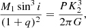
The measurement of K2 depends solely on the FWHM0 of the Hα profile, and can be determined from individual spectra through the following relation Casares 2015:
 (1)
(1)
We used FWHM0 = 990 ± 45 km s−1, the median and the standard deviation of the distribution of individual measurements. Here, the uncertainty in FWHM0 properly reflects orbital variations. Using this FWHM0 estimate and its uncertainty, and performing a Monte Carlo simulation with 105 realisations of Eq. (1), we obtain K2 = 230 ± 17 km s−1.
The binary mass ratio (q) can be estimated using the correlation from Casares 2016, which relates q to the DP-to-FWHM0 ratio:
 (2)
(2)
To estimate q, we applied a symmetric two-Gaussian fit to the weighted average spectrum, yielding  . As shown in Casares 2016, this approach is necessary because individual spectra typically have insufficient S/N for reliable analysis. Moreover, averaging across the orbit helps to minimise distortions from features such as hot spots or disc eccentricities, which could otherwise skew the estimation of q.
The single-Gaussian fit to the average line profile gives FWHM0 = 1001 ± 11 km s−1, while the symmetric two-Gaussian fit yields DP = 586 ± 5 km s−1 and W = 506 ± 9 km s−1. The value of W was then used to estimate the orbital inclination of the system, as described below.
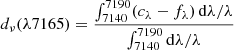
The orbital inclination can be estimated from the depth of the trough (T) between the two peaks of the Hα emission profile using the relation from Casares et al. 2022:
![Mathematical equation: $$ \begin{aligned} i\;[^\circ ] = 93.5\,(6.5)\,T + 23.7\,(2.5), \end{aligned} $$](/articles/aa/full_html/2025/10/aa56452-25/aa56452-25-eq6.gif) (3)
(3)
where T is defined as 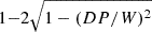 . We corrected T for the effect of instrumental resolution as described in Appendix A of Casares et al. 2022.
Using the values of DP and W calculated earlier, we obtain T = 0.27 ± 0.03 and an inclination of i = 49° ±4°, with uncertainties derived from a Monte Carlo simulation. We verified that the double-peaked Hα profile is affected by contamination from the nearby star also on the slit, with the contamination level depending on seeing. Repeating the analysis using only the average of the five spectra showing less than 1% contamination within 1-σ of the spatial profile of J1910, as determined from two-Gaussian fits to the collapsed spectra near Hα, favours a lower inclination (i ≈ 40°); however, this result should be interpreted with caution owing to the incomplete orbital phase coverage of these spectra. Nevertheless, in Sect. 4.2 we show that the orbital inclination is likely to be much lower.
4. Discussion
4.1. Optical light curve morphology and the orbital period
Our GLS search of the combined 2012 SMARTS, WFC, and Fresno SRO light curves identified a strong signal at 2.26(2) h. At first sight, the photometric variability could be attributed to X-ray heating of the donor star, but several arguments disfavour this scenario in J1910. In particular, a very low mass ratio (q ≲ 0.07) means that the flared outer disc shadows the donor from direct X-rays, so irradiation is inefficient, as argued by Torres et al. 2021 for the very similar MAXI J1659–152. Nevertheless, if X-ray heating of the donor were significant, the low orbital inclination would make its photometric detection unlikely Haswell et al. 2001. Additionally, no narrow emission-line components attributable to an illuminated donor are seen in our spectra. Together, these points indicate an accretion disc origin for the photometric modulation.
The profile of the J1910 light curves (Figs. 4 and 5) suggests that the waveform might be a double-wave (i.e. two-humped), with a fundamental period of ≃4.52 h. Independent support for this possibility comes from the FORS2 Hα radial-velocity wings. For Gaussian separations ≳1850 km s−1, the AOV periodograms show excess power near 4.54 h (0.189 d; Fig. 7 bottom panel). If this interpretation is correct, the double-wave modulation observed in J1910 could well be an ‘early superhump’, a common feature of WZ Sge-type dwarf novae during outburst.
In WZ Sge dwarf novae, it is thought that double-humped modulations arise when the outer disc reaches the 2:1 resonance, producing a two-armed, vertically extended pattern that modulates the optical flux twice per orbit (e.g. Kato 2002; Uemura et al. 2012). This configuration is only attainable for extreme mass ratios, q ≲ 0.08, because the 2:1 resonance radius must lie within the tidal truncation radius. Our spectroscopic estimate for J1910, q = 0.032 ± 0.010, comfortably satisfies this criterion, so the observed double-wave profile could be explained within the early-superhump framework.
The R-band time series of MAXI J1659–152 presented by Kuroda et al. 20107 also exhibits a double-humped profile with an amplitude of ≈0.04 mag that persists for at least the first 18 d after the optical detection of the transient. This modulation is identified by Torres et al. 2021 as a possible early superhump. Analogous behaviour was observed in the black hole transient XTE J1118+480: its 2000−2001 outburst displayed a 4.09-h double-wave superhump just 0.3% longer than its 4.065-h orbital period Uemura et al. 2000; Zurita et al. 2002, while the cataclysmic variable V503 Cyg alternates between single- and double-humped profiles within a single superoutburst Harvey et al. 1995.
Both the amplitude and the lifetime of these modulations align with the canonical properties of early superhumps in WZ Sge systems during outburst: most systems display modulation amplitudes ≲0.05 mag, with occasional extremes up to 0.35 mag Kato 2015, and the signal typically fades within ∼15 d of outburst onset (Nakata et al. 2013, their Table 9). The r-band amplitude of the modulation in J1910 is about 0.02 mag, in line with early superhumps, but persisted for at least 46 d. Additionally, the relatively low amplitude of the modulation also supports a low inclination. As shown by Haswell et al. 2001, the energy released by changes in the disc due to superhumps is negligible compared to the X-ray irradiation during outburst. Thus, detectable superhumps typically require additional asymmetries, such as tilted or warped discs, as invoked by Thomas et al. 2022 for MAXI J1810+070. The modest modulation observed in J1910 suggests no such enhancement, reinforcing the interpretation of a low-inclination geometry (see Sect. 4.2).
However, a reliable determination of the orbital period from the radial velocity curves obtained with ACAM, OSIRIS, or FORS2 was not possible. Consequently, it remains unclear whether the orbital period is close to 2.26 h or approximately twice that value. Using the donor spectral type-orbital period relations from Smith & Dhillon 1998, we estimate spectral types of M5 ± 1 and M2 ± 4 for the shorter and longer periods, respectively. These estimates are too uncertain to meaningfully constrain the orbital period, especially when compared to our measured spectral type of M3–M3.5.
We computed superhump excesses, ϵ, using the q − ϵ relationships from McAllister et al. 2019. For our mass ratio q = 0.032 ± 0.010, we obtain orbital periods of approximately 2.25 and 4.50 h for superhump periods of 2.26 and 4.52 h, respectively, which are slightly shorter than the corresponding superhump period in both cases.
We can estimate the masses of the compact object and the donor star in J1910 using:
 (4)
(4)
where M1 is the mass of the compact object and q = M2/M1, with M2 the mass of the donor star. With our derived values of K2, q, i, and P = 2.26(2) h, a Monte Carlo simulation yields  and
and 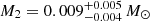 . For twice that period, the inferred values are doubled. The derived masses for both the compact object and the donor are clearly too low. This suggests that either the true orbital period is ∼30 − 40 times longer (∼3 − 4 d), or (more likely) the orbital inclination has been overestimated.
4.2. Inclination constraints and compact object mass
From semi-empirical donor sequences for Roche-lobe-filling stars in cataclysmic variables (e.g. Knigge et al. 2011), the donor’s observed spectral type of M3–3.5 suggests a (conservative) mass of M2 = 0.25 − 0.35 M⊙. To constrain M1 and i, we performed a Monte Carlo simulation incorporating uncertainties in the orbital period, radial velocity semi-amplitude, and mass ratio.
We adopted K2 = 230 ± 17 km s−1, a mass ratio q = 0.032 ± 0.010, and we considered two orbital period scenarios: P = 2.25 ± 0.01 h, and twice that value (P = 4.50 ± 0.03 h). For each of the 105 trials, we computed the mass function (Eq. 4) and solved for M1 and i.
The resulting posterior distributions yield the following median values and 68% confidence intervals:
-
Shorter period (P = 2.25 h):
-
M2 = 0.25 M⊙:
 ,i = 14° ±2°,
 -
M2 = 0.35 M⊙:
 ,i = 13° ±2°.
-
-
Longer period (P = 4.50 h):
-
M2 = 0.25 M⊙:
 ,i = 18° ±3°,
 -
M2 = 0.35 M⊙:
 ,i = 16° ±2°.
-
In both scenarios, the compact object mass falls within the black hole regime, and the derived inclinations are low. In Fig. 10, we present the mass of the compact object as colours for a range of inclinations and donor masses, for the two orbital periods considered.
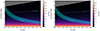 |
Fig. 10. Relationship between the orbital inclination and the mass of the donor star (M2), with the mass of the compact object (M1) represented by colour, for orbital periods of 2.25 (left) and 4.50 h (right). The solid cyan line and cyan shaded area correspond to a mass ratio of 0.032 and its uncertainty, respectively. The light grey dashed line marks M1 = 3 M⊙, and the dark grey triangular areas correspond to M1 < 1.5 M⊙. |
Evidence to support a low inclination comes from the following: Degenaar et al. 2014 reported the absence of ionised disc winds during the softest state of the X-ray outburst, along with a relatively low inner disc temperature (kT ≃ 0.5 keV), in contrast to the kT > 1 keV temperatures typically found in black hole systems; Muñoz-Darias et al. 2013 showed that such cooler disc temperatures are systematically observed at lower inclinations, due to relativistic effects. Additionally, the lack of disc winds is consistent with a low inclination Ponti et al. 2012. Altogether, these findings favour a low orbital inclination for J1910, consistent with our results based on the measured mass ratio and donor mass range inferred from its observed spectral type.
4.3. Alternative scenario: A neutron star accretor
Assuming a canonical neutron star mass of M1 ≈ 1.4 M⊙ and that the M3-type donor is a main-sequence star with a mass of M2 ≈ 0.3 M⊙, the resulting mass ratio would be q ≈ 0.21. This value remains consistent with the observed photometric modulation being due to a superhump–though not an early superhump. In this scenario, the orbital period would be ≈2.25 h, and using the FWHM0-derived K2, the system inclination would be approximately 30°. A challenge to this interpretation comes from the q and i values inferred through empirical correlations with the double-peaked emission lines. One further point worth mentioning is that, under the alternative scenario of a 4.5-h orbital period, the Roche-lobe density constraint suggests the M3-type donor could be a normal main sequence star. In contrast, for a 2.25-h period, the donor would need to be significantly cooler, implying it likely descended from a more massive star that began Roche-lobe overflow while already significantly evolved; this scenario is similar to the evolutionary histories proposed for XTE J1118+480 Haswell et al. 2002 or the cataclysmic variable SDSS J170213.26+322954.1 Littlefair et al. 2006.
5. Conclusions
In this paper, we present a comprehensive study of Swift J1910.2–0546 based on time-series optical photometry and spectroscopy obtained during its 2012 outburst, subsequent decline, and quiescent state. We examine the system’s orbital and stellar parameters, with particular emphasis on constraining the orbital period, inclination, and component masses.
Our analysis of the FORS2 quiescent optical spectrum, dominated by molecular absorption bands characteristic of M dwarfs, has enabled a direct spectral classification of the donor star as M3–3.5. It further suggests that the donor contributes approximately 70% of the red optical flux. Based on the inferred spectral type and the measured reddening E(B − V) = 0.60 ± 0.05, derived from the analysis of DIBs, we estimate a system distance of between 2.8 and 4.0 kpc.
Time-resolved photometry during outburst reveals a photometric modulation with a period of 2.26(2) h, consistent with an early superhump, as observed in extreme mass-ratio accreting systems. This introduces an ambiguity regarding the true orbital period, which may be slightly shorter than twice this photometric period.
The observed double-peaked Hα emission line profile provides an estimate of the binary mass ratio,  , and a radial velocity semi-amplitude of the donor of
  km s−1. However, the inclination derived from the Hα profile, i = 49° ±4°, might be too high compared to independent X-ray-based estimates.
To further constrain the inclination and the mass of the compact object, we considered two possible orbital period scenarios, 2.25 and 4.50 h. We then adopted a conservative donor mass range consistent with the measured spectral type (M2 = 0.25 − 0.35 M⊙). Our Monte Carlo simulations yield a low inclination in the range i = 13° −18° and M1 = 8 − 11 M⊙. Ultimately, we favour the 4.5-h orbital period and a black hole accretor in J1910, but the possibility of there being a neutron star cannot be discarded.
Future time-resolved spectroscopy under excellent seeing conditions (≲0.5″) complemented by r- and/or i-band light curves will be crucial to conclusively determine the orbital period and the true nature of its compact object.
Online version available at https://www.astro.puc.cl/BlackCAT and https://www.sc.eso.org/~jcorral/BlackCAT
We downloaded the SMARTS 0.9-m images from https://astroarchive.noirlab.edu/portal/search
HD 111631 (M0), HD 209290 (M0), HIP 96710 (M1), HD 119850 (M2), HIP 75423 (M2), GJ 109 (M3), HIP 84123 (M3), HD 125455B (M4), and GJ 866 (M5).
Acknowledgments
We thank the referee for a prompt and positive report, and for the constructive suggestions that helped improve the manuscript. We are grateful to Tom Marsh for the use of molly. Beyond his scientific brilliance, Tom was a generous colleague and dear friend. His absence is profoundly felt. PR-G, MAPT, and TM-D acknowledge support by the Agencia Estatal de Investigación del Ministerio de Ciencia e Innovación (MCIN/AEI) and the European Regional Development Fund (ERDF) under grant PID2021–124879NB–I00. DMS acknowledges support via a Ramón y Cajal Fellowship RYC2023–044941. PGJ is supported by the European Union (ERC, Starstruck, 101095973). Views and opinions expressed are however those of the author(s) only and do not necessarily reflect those of the European Union or the European Research Council Executive Agency. Neither the European Union nor the granting authority can be held responsible for them. PAC acknowledges the Leverhulme Trust for an Emeritus Fellowship. PS and DMR are supported by Tamkeen under the NYU Abu Dhabi Research Institute grant CASS. This research has made use of the SIMBAD database, the VizieR catalogue access tool, and Aladin sky atlas (CDS, Strasbourg Astronomical Observatory, France). This research has also made use of IRAF, which is distributed by the National Optical Astronomy Observatory, which is operated by the Association of Universities for Research in Astronomy (AURA) under a cooperative agreement with the National Science Foundation. This research is based on data obtained from the Astro Data Archive at NSF’s NOIRLab. These data are associated with observing program NOAO 2012A–0424 (PI C. Britt). NOIRLab is managed by the Association of Universities for Research in Astronomy (AURA) under a cooperative agreement with the National Science Foundation. Based on observations collected at the European Organisation for Astronomical Research in the Southern Hemisphere under ESO programme(s) 097.D–0270 (PI P. Jonker), and observed with GTC under program GTC38-16B (PI J. Casares). The WHT and INT are operated by the Isaac Newton Group of Telescopes. These telescopes together with the GTC are installed at the Spanish Observatorio del Roque de los Muchachos of the Instituto de Astrofísica de Canarias, on the island of La Palma. This research used photometry taken at Fresno State’s station at Sierra Remote Observatories. We thank Dr. Greg Morgan, Dr. Melvin Helm, and Dr. Keith Quattrocchi, and the other SRO observers for creating this fine facility. This research made use of APLpy Robitaille & Bressert 2012, SciPy Virtanen et al. 2020 and AstroPy Astropy Collaboration 2022.
References
- Astropy Collaboration (Price-Whelan, A. M., et al.) 2022, ApJ, 935, 167 [NASA ADS] [CrossRef] [Google Scholar]
- Belloni, T. M. 2010, ArXiv e-prints [arXiv:1007.5404] [Google Scholar]
- Berry, R., & Burnell, J. 2005, The Handbook of Astronomical Image Processing (Richmond, Virginia: Willman-Bell), 2 [Google Scholar]
- Boeshaar, P. C. 1976, Ph.D. Thesis, The Ohio State University [Google Scholar]
- Britt, C. T., Johnson, C. C. B., & Hynes, R. I. 2012, ATel, 4195 [Google Scholar]
- Cardelli, J. A., Clayton, G. C., & Mathis, J. S. 1989, ApJ, 345, 245 [Google Scholar]
- Casares, J. 2015, ApJ, 808, 80 [NASA ADS] [CrossRef] [Google Scholar]
- Casares, J. 2016, ApJ, 822, 99 [NASA ADS] [CrossRef] [Google Scholar]
- Casares, J., Rodríguez-Gil, P., Zurita, C., et al. 2012, ATel, 4347 [Google Scholar]
- Casares, J., Muñoz-Darias, T., Torres, M. A. P., et al. 2022, MNRAS, 516, 2023 [NASA ADS] [CrossRef] [Google Scholar]
- Cenko, S. B., & Ofek, E. O. 2012, ATel, 4146 [Google Scholar]
- Cepa, J., Aguiar-Gonzalez, M., Bland-Hawthorn, J., et al. 2003, SPIE Conf. Ser., 4841, 1739 [NASA ADS] [Google Scholar]
- Chambers, K. C., Magnier, E. A., Metcalfe, N., et al. 2016, ArXiv e-prints [arXiv:1612.05560] [Google Scholar]
- Charles, P. A., & Coe, M. J. 2006, Compact Stellar X-ray Sources (Cambridge: Cambridge University Press), 215 [Google Scholar]
- Charles, P., Cornelisse, R., & Casares, J. 2012, ATel, 4210 [Google Scholar]
- Corral-Santana, J. M., Casares, J., Muñoz-Darias, T., et al. 2016, A&A, 587, A61 [NASA ADS] [CrossRef] [EDP Sciences] [Google Scholar]
- Czesla, S., Schröter, S., Schneider, C. P., et al. 2019, Astrophysics Source Code Library [record ascl:1906.010] [Google Scholar]
- Degenaar, N., Maitra, D., Cackett, E. M., et al. 2014, ApJ, 784, 122 [Google Scholar]
- Done, C., Gierliński, M., & Kubota, A. 2007, A&ARv, 15, 1 [Google Scholar]
- Fender, R. P., Belloni, T. M., & Gallo, E. 2004, MNRAS, 355, 1105 [NASA ADS] [CrossRef] [Google Scholar]
- Gaia Collaboration (Vallenari, A., et al.) 2023, A&A, 674, A1 [NASA ADS] [CrossRef] [EDP Sciences] [Google Scholar]
- Green, G. M., Schlafly, E., Zucker, C., Speagle, J. S., & Finkbeiner, D. 2019, ApJ, 887, 93 [NASA ADS] [CrossRef] [Google Scholar]
- Güver, T., & Özel, F. 2009, MNRAS, 400, 2050 [Google Scholar]
- Hamuy, M., Walker, A. R., Suntzeff, N. B., et al. 1992, PASP, 104, 533 [NASA ADS] [CrossRef] [Google Scholar]
- Hamuy, M., Suntzeff, N. B., Heathcote, S. R., et al. 1994, PASP, 106, 566 [NASA ADS] [CrossRef] [Google Scholar]
- Harvey, D., Skillman, D. R., Patterson, J., & Ringwald, F. A. 1995, PASP, 107, 551 [Google Scholar]
- Haswell, C. A., King, A. R., Murray, J. R., & Charles, P. A. 2001, MNRAS, 321, 475 [NASA ADS] [CrossRef] [Google Scholar]
- Haswell, C. A., Hynes, R. I., King, A. R., & Schenker, K. 2002, MNRAS, 332, 928 [Google Scholar]
- Hosokawa, R., Murata, K. L., Niwano, M., et al. 2022, ATel, 15226 [Google Scholar]
- Jiménez-Ibarra, F., Muñoz-Darias, T., Armas Padilla, M., et al. 2019, MNRAS, 484, 2078 [CrossRef] [Google Scholar]
- Kato, T. 2002, PASJ, 54, L11 [NASA ADS] [Google Scholar]
- Kato, T. 2015, PASJ, 67, 108 [NASA ADS] [CrossRef] [Google Scholar]
- Kimura, M., Tomida, H., Nakahira, S., et al. 2012, ATel, 4198 [Google Scholar]
- Knigge, C., Baraffe, I., & Patterson, J. 2011, ApJS, 194, 28 [Google Scholar]
- Kong, A. K. H. 2022, ATel, 15229 [Google Scholar]
- Krełowski, J., Galazutdinov, G., Godunova, V., & Bondar, A. 2019, Acta Astron., 69, 159 [Google Scholar]
- Krimm, H. A., Barthelmy, S. D., Baumgartner, W., et al. 2012, ATel, 4139 [Google Scholar]
- Kuroda, D., Hanayama, H., Miyaji, T., et al. 2010, The First Year of MAXI: Monitoring Variable X-ray Sources, 4 [Google Scholar]
- Lan, T.-W., Ménard, B., & Zhu, G. 2015, MNRAS, 452, 3629 [Google Scholar]
- Lasota, J.-P. 2001, New Astron. Rev., 45, 449 [Google Scholar]
- Littlefair, S. P., Dhillon, V. S., Marsh, T. R., & Gänsicke, B. T. 2006, MNRAS, 371, 1435 [Google Scholar]
- Lloyd, C., Oksanen, A., Starr, P., Darlington, G., & Pickard, R. 2012, ATel, 4246 [Google Scholar]
- López, K. M., Jonker, P. G., Torres, M. A. P., et al. 2019, MNRAS, 482, 2149 [CrossRef] [Google Scholar]
- Marsh, T. R. 1990, ApJ, 357, 621 [NASA ADS] [CrossRef] [Google Scholar]
- McAllister, M., Littlefair, S. P., Parsons, S. G., et al. 2019, MNRAS, 486, 5535 [NASA ADS] [CrossRef] [Google Scholar]
- Munari, U., Tomasella, L., Fiorucci, M., et al. 2008, A&A, 488, 969 [NASA ADS] [CrossRef] [EDP Sciences] [Google Scholar]
- Muñoz-Darias, T., Coriat, M., Plant, D. S., et al. 2013, MNRAS, 432, 1330 [Google Scholar]
- Muñoz-Darias, T., Jiménez-Ibarra, F., Panizo-Espinar, G., et al. 2019, ApJ, 879, L4 [CrossRef] [Google Scholar]
- Nakahira, S., Ueda, Y., Takagi, T., et al. 2012, ATel, 4273 [Google Scholar]
- Nakahira, S., Negoro, H., Shidatsu, M., et al. 2014, PASJ, 66, 84 [Google Scholar]
- Nakata, C., Ohshima, T., Kato, T., et al. 2013, PASJ, 65, 117 [Google Scholar]
- Oke, J. B. 1990, AJ, 99, 1621 [Google Scholar]
- Ponti, G., Fender, R. P., Begelman, M. C., et al. 2012, MNRAS, 422, L11 [NASA ADS] [CrossRef] [Google Scholar]
- Ratti, E. M., Steeghs, D. T. H., Jonker, P. G., et al. 2012, MNRAS, 420, 75 [Google Scholar]
- Rau, A., Greiner, J., & Schady, P. 2012, ATel, 4144 [Google Scholar]
- Robitaille, T., & Bressert, E. 2012, Astrophysics Source Code Library [record ascl:1208.017] [Google Scholar]
- Rodríguez-Gil, P., Shahbaz, T., Marsh, T. R., et al. 2015, MNRAS, 452, 146 [CrossRef] [Google Scholar]
- Rodríguez-Gil, P., Shahbaz, T., Torres, M. A. P., et al. 2020, MNRAS, 494, 425 [CrossRef] [Google Scholar]
- Russell, T. D., Soria, R., Motch, C., et al. 2014, MNRAS, 439, 1381 [CrossRef] [Google Scholar]
- Saikia, P., Russell, D. M., Alabarta, K., et al. 2022, ATel, 15303 [Google Scholar]
- Saikia, P., Russell, D. M., Pirbhoy, S. F., et al. 2023a, ApJ, 949, 104 [Google Scholar]
- Saikia, P., Russell, D. M., Pirbhoy, S. F., et al. 2023b, MNRAS, 524, 4543 [Google Scholar]
- Schlafly, E. F., & Finkbeiner, D. P. 2011, ApJ, 737, 103 [Google Scholar]
- Schneider, D. P., & Young, P. 1980, ApJ, 238, 946 [NASA ADS] [CrossRef] [Google Scholar]
- Schwarzenberg-Czerny, A. 1996, ApJ, 460, L107 [NASA ADS] [Google Scholar]
- Smith, D. A., & Dhillon, V. S. 1998, MNRAS, 301, 767 [NASA ADS] [CrossRef] [Google Scholar]
- Stellingwerf, R. F. 1978, ApJ, 224, 953 [Google Scholar]
- Stetson, P. B. 1987, PASP, 99, 191 [Google Scholar]
- Thomas, J. K., Charles, P. A., Buckley, D. A. H., et al. 2022, MNRAS, 509, 1062 [Google Scholar]
- Tominaga, M., Nakahira, S., Negoro, H., et al. 2022, ATel, 15214 [Google Scholar]
- Tonry, J. L., Stubbs, C. W., Lykke, K. R., et al. 2012, ApJ, 750, 99 [Google Scholar]
- Torres, M. A. P., Jonker, P. G., Casares, J., Miller-Jones, J. C. A., & Steeghs, D. 2021, MNRAS, 501, 2174 [NASA ADS] [CrossRef] [Google Scholar]
- Trelawny, D. T. 2013, Master’s Thesis, California State University, USA [Google Scholar]
- Truss, M. R., Wynn, G. A., Murray, J. R., & King, A. R. 2002, MNRAS, 337, 1329 [Google Scholar]
- Uemura, M., Kato, T., Matsumoto, K., et al. 2000, PASJ, 52, L15 [Google Scholar]
- Uemura, M., Kato, T., Ohshima, T., & Maehara, H. 2012, PASJ, 64, 92 [Google Scholar]
- Usui, R., Nakahira, S., Tomida, H., et al. 2012, ATel, 4140 [Google Scholar]
- VanderPlas, J. T. 2018, ApJS, 236, 16 [Google Scholar]
- Verro, K., Trager, S. C., Peletier, R. F., et al. 2022, A&A, 660, A34 [NASA ADS] [CrossRef] [EDP Sciences] [Google Scholar]
- Virtanen, P., Gommers, R., Oliphant, T. E., et al. 2020, Nat. Meth., 17, 261 [Google Scholar]
- Wade, R. A., & Horne, K. 1988, ApJ, 324, 411 [Google Scholar]
- Wenger, M., Ochsenbein, F., Egret, D., et al. 2000, A&AS, 143, 9 [NASA ADS] [CrossRef] [EDP Sciences] [Google Scholar]
- Williams, D., Motta, S., Rhodes, L., et al. 2022, ATel, 15219 [Google Scholar]
- Yanes-Rizo, I. V., Torres, M. A. P., Casares, J., et al. 2025, A&A, 694, A119 [NASA ADS] [CrossRef] [EDP Sciences] [Google Scholar]
- Young, P., & Schneider, D. P. 1981, ApJ, 247, 960 [NASA ADS] [CrossRef] [Google Scholar]
- Zechmeister, M., & Kürster, M. 2009, A&A, 496, 577 [CrossRef] [EDP Sciences] [Google Scholar]
- Zhang, G. B., Bernardini, F., Russell, D. M., et al. 2019, ApJ, 876, 5 [Google Scholar]
- Zurita, C., Casares, J., Shahbaz, T., et al. 2002, MNRAS, 333, 791 [CrossRef] [Google Scholar]
All Tables
Comparison of the average FWHM0 and EW of the Hα line measured in the spectra of J1910 taken during outburst and quiescence.
All Figures
|
Fig. 1. VLT/FORS2 I-band acquisition image obtained during quiescence. J1910 is marked with a red cross at the centre of the 1.2′ field. North is up, east is to the left. |
| In the text | |
|
Fig. 2. Evolution of the 2012 outburst. X-ray data are shown as a grey line, while the R-, V-, and i′-band magnitudes published by Saikia et al. 2023a are represented by red diamonds, green squares, and black circles, respectively. Time-series photometry obtained with the SMARTS 0.9-m and INT/WFC in the r-band is marked with blue triangles, whereas the time of the WHT/ACAM spectra are indicated by orange arrows. Clear-filter photometry from Fresno SRO is marked by vertical red lines. |
| In the text | |
|
Fig. 3. Average spectra of J1910 during outburst from the first (upper; blue) and second (lower; red) nights, obtained with ACAM after continuum normalisation. The Balmer series down to Hδ is visible, exhibiting both emission and absorption components. Zoomed-in regions show the areas around Hα and Hβ. He I and He II lines are also present and identified in the spectra, along with several diffuse interstellar bands marked with orange bars. |
| In the text | |
|
Fig. 4. Top panel: r-band light curves from SMARTS 0.9-m and INT/WFC, expressed as flux ratios and magnitudes, relative to the comparison star. Middle panels: SMARTS light curve (top left) and INT/WFC light curves from the first three nights when J1910 maintained an almost constant flux level, after subtracting the nightly averages. The red dashed curve represents the best-fit sine wave with a period corresponding to the highest peak in the periodogram shown below. Bottom left panel: GLS periodogram of the four r-band light curves displayed in the middle panels (4, 9, 10, and 11 Jun. 2012). The highest peak corresponds to a period of 0.0941 d ( = 2.26 h). Bottom middle and right panels: The four light curves folded on this period and twice that value. The pale blue points represent the unbinned data, while the purple points are binned data across 40 phase intervals. The zero phase corresponds to the HJD of the first data point and a full cycle is repeated for continuity. |
| In the text | |
|
Fig. 5. Top panel: Clear-filter light curves from Fresno SRO on 27, 28 June, and 10, 20 July 2012. Middle panels: Zoomed-in view of the four light curves. The red dashed curve represents the best-fit sine wave with a period corresponding to the highest peak in the periodogram shown below. Bottom left panel: GLS periodogram of the four clear-filter light curves shown in the middle panels after subtraction of nightly averages. The highest peak corresponds to a period of 0.0948 d (2.275 h). Bottom middle and right panels: The four light curves folded on this period and twice that value. The pale blue points represent the unbinned data, while the purple points are binned data across 40 phase intervals. Zero phase is the HJD of the first data point. |
| In the text | |
|
Fig. 6. Top panel: Average GTC/OSIRIS spectrum of J1910 during quiescence. The bluer part has been trimmed due to unreliable correction for the instrumental response. Although veiled by slit contamination from the two nearby stars (see Fig. 1), caused by seeing ≳1″, TiO absorption bands characteristic of M-stars are present in the 6800−7200 Å wavelength range. Bottom panel: The detection of an M-star donor is confirmed by the telluric-corrected, average VLT/FORS2 spectrum also obtained during quiescence. Both average spectra were dereddened using E(B − V) = 0.6 (see Sect. 3.4), and the FORS2 spectrum was smoothed with a Savitzky-Golay filter, employing a window length of nine data points and a third-order fitting polynomial for illustrative purposes. |
| In the text | |
|
Fig. 7. Top panel: Best sine-fit periods derived from the radial velocity curves of the Hα emission line in the OSIRIS spectra, as a function of the double-Gaussian separation used in the velocity extraction. The shaded horizontal band indicates the periods derived from the light curves. Error bars represent 1σ uncertainties. Bottom panel: Periods corresponding to the highest peaks in the GLS (blue circles) and AOV (orange squares) periodograms derived from the quiescent FORS2 Hα radial velocity curves, as a function of the Gaussian separation used to extract the velocities. The period search was restricted to the range 0.068−0.25 d. The lower shaded horizontal band marks the periods observed in the photometric light curves, while the upper band corresponds to twice these values. |
| In the text | |
|
Fig. 8. Average of the 15 FORS2 spectra obtained during quiescence. The profile of the Hα emission line is double-peaked. |
| In the text | |
|
Fig. 9. Fractional depth of the TiO λ7665 band as a function of the TiO band deficit ratio for J1910 and comparison M-type stars. Blue dots indicate X-shooter Library M dwarfs, while grey triangles correspond to those used by Marsh 1990. |
| In the text | |
|
Fig. 10. Relationship between the orbital inclination and the mass of the donor star (M2), with the mass of the compact object (M1) represented by colour, for orbital periods of 2.25 (left) and 4.50 h (right). The solid cyan line and cyan shaded area correspond to a mass ratio of 0.032 and its uncertainty, respectively. The light grey dashed line marks M1 = 3 M⊙, and the dark grey triangular areas correspond to M1 < 1.5 M⊙. |
| In the text | |
Current usage metrics show cumulative count of Article Views (full-text article views including HTML views, PDF and ePub downloads, according to the available data) and Abstracts Views on Vision4Press platform.
Data correspond to usage on the plateform after 2015. The current usage metrics is available 48-96 hours after online publication and is updated daily on week days.
Initial download of the metrics may take a while.