| Issue |
A&A
Volume 703, November 2025
|
|
|---|---|---|
| Article Number | A30 | |
| Number of page(s) | 7 | |
| Section | Astrophysical processes | |
| DOI | https://doi.org/10.1051/0004-6361/202554318 | |
| Published online | 31 October 2025 | |
Lense-Thirring precession of neutron-star accretion flows: Relativistic versus classical precession
1
Research Centre for Computational Physics and Data Processing, Institute of Physics, Silesian University in Opava, Bezručovo nám. 13, CZ-746 01 Opava, Czech Republic
2
Nicolaus Copernicus Astronomical Center of the Polish Academy of Sciences, Bartycka 18, 00-716 Warsaw, Poland
3
Astronomical Institute of the Czech Academy of Sciences, Boční II 1401, CZ-14100 Prague, Czech Republic
⋆ Corresponding author: This email address is being protected from spambots. You need JavaScript enabled to view it.
Received:
28
February
2025
Accepted:
10
August
2025
Abstract
The vertical (Lense-Thirring) precession of the innermost accretion flows has been discussed as a sensitive indicator of the rotational properties of neutron stars (NSs) and their equation of state because it vanishes for a non-rotating star. For this work we applied the Hartle-Thorne spacetimes to study the frequencies of the precession for both geodesic and non-geodesic (fluid) flows. We built on previous findings of the effect of the NS quadrupole moment, which revealed the importance of the interplay between the relativistic and classical precession. Because of this interplay, the widely used Lense-Thirring metric, linear in the NS angular momentum, is insufficient to calculate the behaviour of the precession frequency across an astrophysically relevant range of NS angular momentum values. We find that even for moderately oblate NSs, the dependences of the precession frequency on the NS angular momentum at radii within the innermost accretion region have maxima that occur at relatively low values of the NS angular momentum. We conclude that very different groups of accreting NSs – slow and fast rotators – can display the same precession frequencies. This may explain the lack of evidence for a correlation between the frequencies of the observed low-frequency quasiperiodic oscillations and the NS spin. In our work we provide a full general description of precession behaviour, and also examples that assume specific NS and quark star (MIT bag) equations of state. Our calculations are reproducible using the associated Wolfram Mathematica notebook.
Key words: stars: neutron / X-rays: binaries
© The Authors 2025
 Open Access article, published by EDP Sciences, under the terms of the Creative Commons Attribution License (https://creativecommons.org/licenses/by/4.0), which permits unrestricted use, distribution, and reproduction in any medium, provided the original work is properly cited.
This article is published in open access under the Subscribe to Open model. This email address is being protected from spambots. You need JavaScript enabled to view it. to support open access publication.
1. Introduction
Neutron star low-mass X-ray binaries (NS LMXBs), which consist of an NS accreting matter from a less massive companion star, are invaluable for studying extreme environments and fundamental physics of dense matter (van der Klis 2006; Lewin & van der Klis 2010). Among the various phenomena observed in these systems, the X-ray variability exhibits a rich and diverse phenomenology.
On short timescales, NS LMXBs often display a complex of quasi-periodic oscillations (QPOs) in the low- and high-frequency (LF and HF) bands. These features, represented by multiple peaks in the Fourier power-density spectra, span from a few hertz to a few tens of hertz for LF QPOs and from a few hundred hertz up to 1.3 kHz for HF QPOs. The HF QPOs often consist of two peaks, one of which is sometimes highly coherent, with quality factors (the height of the peak at its half-width) reaching up to Q ∼ 300, and high root mean square amplitude reaching up to 30% (Barret et al. 2005b, 2006; Barret & Vaughan 2012). The peaks within the LF QPO complex have relatively low coherence, but still notable amplitudes (Barret et al. 2005a; Méndez 2006; Barret & Vaughan 2012). Similar behaviour is observed in the black hole LMXBs. However, the QPOs are weaker there, and the HF QPOs represent somewhat elusive features with small amplitudes and coherences. Commonly to both classes of sources, HF and LF QPO frequencies seem to be well correlated (Stella & Vietri 1999; Mauche 2002; van der Klis 2006; Remillard & McClintock 2006; Belloni & Motta 2016).
It is frequently assumed that the QPOs emerge from the orbital motion in the vicinity of the central NS (Barret et al. 2006; van der Klis 2006). A large variety of orbital models of QPOs have been proposed assuming either local effects within the accretion disc or the global motion of the disc itself (e.g., Kluźniak et al. 1990; Karas 1999; Čadež et al. 2008; Kato 2001; Wagoner et al. 2001). Many of them deal with an inner thick accretion flow (torus) and its epicyclic oscillations (Abramowicz & Kluźniak 2001; Kluźniak & Abramowicz 2001), or other modes of torus oscillations (Rezzolla et al. 2003a,b; Blaes et al. 2006; Fragile et al. 2016; Ingram & Done 2010; Mishra et al. 2017; de Avellar et al. 2018).
At the end of the millennium, the relativistic precession (RP) model was proposed (Stella & Vietri 1998, 1999; Stella et al. 1999), which relates the HF and LF QPOs to the radial (periastron) and vertical (Lense-Thirring, LT) precession of inhomogeneities orbiting within the innermost accretion flow. They noticed that the vertical precession emerges as a critical tool for probing the characteristics and internal structure of NSs. Notably, the precession driven by the relativistic frame-dragging effects of the NS’s rotation should be absent in non-rotating NSs, making it possibly a distinctive indicator of NS rotation and equation of state (EoS). The concept of the RP model was later discussed in many works, including Ingram et al. (2009), Ingram & Done (2010, 2011), Middleton et al. (2019), Fragile (2020), and Bollimpalli et al. (2024), where the authors focused on the vertical precession along with related results of numerical simulations of oscillations of accretion flows and their comparison with observations of LF QPOs.
The predictions of the RP model and models predicting similar observable frequencies have been extensively studied in relation to both HF and LF QPOs in a variety of astrophysical sources (Stella & Vietri 1998, 1999; Motta et al. 2012, 2014, 2022; Stuchlík & Kološ 2016a,b; Török et al. 2016a,b, 2018; van Doesburgh et al. 2018; van Doesburgh & van der Klis 2020; Kotrlová et al. 2020; Maselli et al. 2020). While in the former case the expected frequencies in NS sources seem to agree with the observations (Belloni et al. 2007; Lin et al. 2011; Török et al. 2022), in the latter case a lack of strong correlation between the frequencies of the LF QPOs and the NS spin was found (Altamirano et al. 2012; van Doesburgh & van der Klis 2017, 2019; du Buisson et al. 2021).
In our previous works, we studied the oscillations of inner fluid accretion flow using an analytic approach, focusing on the radial precession and its possible relation to the HF QPOs (Török et al. 2016a, 2022). In the recent papers of Matuszková et al. (2024a,b), we further provided tools to investigate the vertical precession. Here we follow our most recent work and investigate the behaviour of the vertical precession frequencies.
2. Approach to rotating oblate compact stars
In the context of the RP model, the vertical epicyclic frequency and the frequency of LT precession of the geodesic motion around rotating oblate NSs were investigated by Morsink & Stella (1999), who calculated the associated post-Newtonian formulae, studied numerical models of rotating NSs, and compared the model predictions with the data. The behaviour of the precession frequencies and possible observable signatures of the NS structure were later investigated by Pappas (2012), who focused on the effects of multipole moments of spacetime. The study emphasised that, even for realistic NS models, the dependence of the precession frequency on the rotational frequency of the NS can be non-monotonic, and that the vertical epicyclic frequency can be greater than the Keplerian (see also Pappas & Apostolatos 2012; Pappas 2015).
The complex physics behind the behaviour of the geodesic epicyclic frequencies around rotating oblate compact stars was further explored in the works of Kluźniak & Rosińska (2013, 2014) and Gondek-Rosińska et al. (2014), who, motivated by the works of Zdunik & Gourgoulhon (2001) and Amsterdamski et al. (2002), calculated analytical formulae describing the epicyclic frequencies of rotating oblate bodies in Newtonian gravity, namely the Maclaurin spheroids, and compared them with those calculated for rotating quark stars (QSs) using a numerical general-relativistic approach. They showed the importance of the interplay between the relativistic effects and the effects arising purely from the spatial distribution of the gravitating mass. In terms of the LT precession, this interplay manifests itself as a competition between the relativistic and classical precession. The results of these works were consequently extended in some aspects by Tsang & Pappas (2016), who focused on the self-trapping of discoseismic corrugation modes in NS spacetimes, and Bollimpalli (2022), who calculated epicyclic frequencies in the case of Newtonian stars composed of concentric spheroids.
Here, we generalised the previous results. Using a fully analytic, general relativistic approach, we examined LT precession in relation to any rotating, oblate compact stars, including NSs and QSs. Furthermore, we investigated not only frequencies associated with geodesic motion, but also those associated with non-geodesic fluid flows.
2.1. Spacetime
We studied spacetime geometry around a rotating axisymmetric compact object governed by general relativity in terms of the Schwarzschild coordinates {t, r, θ, φ}. The corresponding metric tensor captures the curvature induced by the star’s mass and rotation, and is represented by1
 (1)
(1)
To handle the calculation on the NS spacetime background, the LT metric (Lense & Thirring 1918) is often used. However, this metric is only linear in the NS angular momentum. Here we adopt the Hartle-Thorne (HT) metric (Hartle 1967; Hartle & Thorne 1968), which takes into account the star’s mass M, angular momentum J, and quadrupole moment Q. To simplify the expressions, we use the dimensionless angular momentum and quadrupole moment, j = J/M2 and q = Q/M3. The components of the HT metric in notation adopted here (Abramowicz et al. 2003; Urbancová et al. 2019) are, along with the components of the linear metric, given in a Wolfram Mathematica notebook associated with this work2.
2.2. Quadrupole parameter
In principle, a non-rotating NS can have non-zero oblateness. Here, we assume the oblateness to be entirely rotationally induced, and thus to vanish when the angular momentum of the star reaches zero. To study the effects of the oblateness and angular momentum on the orbital motion, we utilise the quadrupole parameter,
 (2)
(2)
This quantity is determined by the given NS EoS and M and does not depend on the NS rotational frequency (e.g., Urbancová et al. 2019). Furthermore, in terms of the spacetime geometry, its value determines whether the influence of the gtφ component of the metric tensor and the associated frame-dragging effects, which are linear in j, dominate or can be overtaken by the other components. This occurs as j increases, and as the effects given purely by the spatial distribution of the gravitating mass associated with j2 become important.
2.3. Range of spacetime parameters
The range of parameters considered here is constrained by the observed properties of neutron stars in accreting systems, with masses ranging from 1.4 M⊙ to 2.5 M⊙ (Strohmayer et al. 1996; Lattimer & Prakash 2001) and rotational frequencies corresponding to millisecond pulsars. Previous studies of NS models have shown that the maximum dimensionless angular momentum is approximately jmax ≈ 0.7, with a corresponding quadrupole parameter  ranging from
  for a very massive (compact) NS to
  for a low-mass NS depending on the NS equation of state (Lo & Lin 2011; Urbancová et al. 2019).
3. Orbital motion
Properties of the orbital motion of a free test particle provide basic insights into gravitational interactions and the behaviour of accretion flows near compact objects3. In the simple case of Schwarzschild spacetime, which is spherically symmetric and static, two fundamental orbital frequencies corresponding to a radially perturbed circular orbital motion exist:
The azimuthal (Keplerian) angular frequency ΩK, and the radial epicyclic angular frequency Ωr,
 (3)
(3)
Accordingly, the relativistic precession arises, which manifests as a gradual advance in the orbit’s periastron, with angular frequency
 (4)
(4)
In the HT spacetimes, the azimuthal and radial frequencies are then modified due to the additional frame-dragging and quadrupole contributions associated with the slow NS rotation. The azimuthal frequency reads (Abramowicz et al. 2003)
![Mathematical equation: $$ \begin{aligned} \Omega _{\mathrm{K} }= \frac{M^{1/2}}{r^{3/2}} \left[ 1 - j \frac{M^{3/2}}{r^{3/2}} + j^2 \alpha _1 (r) + q \alpha _2 (r) \right], \end{aligned} $$](/articles/aa/full_html/2025/11/aa54318-25/aa54318-25-eq8.gif) (5)
(5)
and the radial frequency reads (Abramowicz et al. 2003)
![Mathematical equation: $$ \begin{aligned} \Omega _r^2 = \frac{M}{r^3}\left( 1- \frac{6M}{r} \right) \left[ 1 + j \gamma _1(r) - j^2 \gamma _2(r) - q \gamma _3(r) \right]. \end{aligned} $$](/articles/aa/full_html/2025/11/aa54318-25/aa54318-25-eq9.gif) (6)
(6)
Here the terms α1(r), α2(r), γ1(r), γ2(r), and γ3(r) reflect the effects induced by the NS rotation and are provided in their complete form in the associated Wolfram Mathematica notebook.
4. LT precession
In Schwarzschild geometry, the vertical epicyclic frequency equals the Keplerian frequency, Ωθ = ΩK. However, in the HT geometry, the vertical epicyclic frequency is different due to the breaking of spherical symmetry and takes the form (Abramowicz et al. 2003)
![Mathematical equation: $$ \begin{aligned} \Omega _\theta ^2 = \frac{M}{r^3} \left[ 1 - j \delta _1(r) + j^2 \delta _2(r) + q \delta _3(r) \right], \end{aligned} $$](/articles/aa/full_html/2025/11/aa54318-25/aa54318-25-eq10.gif) (7)
(7)
where the terms δ1(r), δ2(r), and δ3(r) are again provided in the Wolfram Mathematica notebook.
This induces LT precession with a frequency given by
 (8)
(8)
In the LT spacetime, this precession causes the orbital plane to precess in the direction of the NS’s rotation. The profiles of the oscillation frequencies of a free test particle corresponding to the frequencies of axisymmetric oscillations of slender tori are shown in the upper panels of Figure 1, and the bottom panels illustrate the behaviour of the precession frequencies. Within the figure, we assume a moderately rotating star and compare the frequencies calculated within the LT metric (panels a) to those calculated for the Kerr limit of the HT spacetimes corresponding to an extremely compact NS (that nearly coincide with those calculated for the Kerr metric, panels b), and those calculated for a highly oblate NS described in the HT spacetime (panels c).
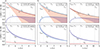 |
Fig. 1. Frequencies of orbital motion around rotating NSs. a) NS spacetime approximated using the LT metric. b) Spacetime of extremely compact NSs approximated using the Kerr limit of the HT metric. c) Spacetime of highly oblate NSs approximated by the HT metric. The upper panels show the Keplerian and (axisymmetric) epicyclic frequencies. The bottom panels show the precession frequencies. The solid lines correspond to the frequencies of a test particle motion and slender tori. The colour-shaded regions indicate frequencies relevant to the non-geodesic flows of non-slender tori. The dashed lines in panel b indicate the frequencies of a test particle motion in the Kerr spacetime calculated using the appropriate coordinate transformation. |
4.1. Fluid flows
To inspect the behaviour of the fluid flow oscillations, we follow Matuszková et al. (2024a,b) and consider an inner accretion torus orbiting an NS. The adopted torus model assumes a fluid with constant specific angular momentum throughout the flow, with Keplerian value at the torus centre. A polytropic equation of state further describes the fluid. In contrast to the oscillation frequencies of a free test particle, the oscillations of such a fluid torus involve additional corrections due to the internal pressure forces. The oscillation frequencies are given as
 (9)
(9)
where  represents the epicyclic frequencies of a free test particle, i = {r, θ}, m denotes the oscillation mode, parameter β defines the torus thickness, and
  represents the second-order pressure corrections. All the formulae that express these terms explicitly are provided within the associated Wolfram Mathematica notebook.
In the specific case of the lowest-order non-axisymmetric oscillations (m = −1), the oscillatory modes of the torus can be seen as torus precession in the corresponding radial or vertical direction, with frequencies4
 (10)
(10)
which, in the limit of a slender torus (β = 0), are equal to those corresponding to the test particle motion,
 (11)
(11)
The oscillation frequencies of fluid flows of the non-slender tori are shown in the upper panels of Figure 1. Similarly, the frequencies of the periastron and LT precessions of these flows are shown in the lower panels of Figure 1.
4.2. Inner parts of the flow
Within Figure 1, we mark four distinct radii. First, there is the position of the innermost stable circular orbit, rISCO, where the geodesic radial epicyclic frequency vanishes,
 (12)
(12)
Then, there is the radius close to ISCO, r3 : 1, where νθ = 3νr, and the radius r2 : 1, where νθ = 2νr and νr reaches a maximum. When the NS spacetime differ from the case of j = 0, for the maximum of νr there is still νθ ≈ 2νr (Török et al. 2008). Last, we mark the radius where 2νθ = 3νr. Next, we inspect how νLT changes with the NS spin along these four radii, which cover the innermost parts of an accretion flow.
5. Effects of spin
As elaborated in the works of Gondek-Rosińska et al. (2014), Tsang & Pappas (2016), and Urbancová et al. (2019), for rotating oblate stars, the geodesic vertical epicyclic frequency exceeds the Keplerian frequency for sufficiently high values of j and q. In this situation, as illustrated in Figs. 1c and 2, which are drawn for j = 0.35, the LT precession changes orientation at a radius close to the ISCO. Its frequency values are then negative below this radius and positive above it, while νLT again vanishes at infinity. Figure 2 further illustrates the presence of a local radial maximum of the precession frequency. This maximum may be present even when the LT precession frequency only vanishes at infinity and not at radii close to the ISCO.
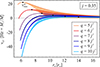 |
Fig. 2. Change in the orientation of the LT precession and behaviour of local frequency maxima shown for j = 0.35. As in Figure 1, the solid lines correspond to the frequencies of test particle motion and slender tori, while the shaded regions indicate the frequencies relevant to non-geodesic flows. The solid black circles indicate local maxima of the geodesic precession frequency, νmax0. |
Making use of equations (9), (10), (12), and the condition
 (13)
(13)
we find that, for any given  , the precession frequency at the ISCO exhibits a maximum in relation to spin, νISCOmax, which occurs at
 (14)
(14)
In Figure 3a, we show several examples of the behaviour of νLT(j, r = rISCO) for realistic values of  . The displayed frequencies are relevant for the inner edge of a thin accretion disc and for a slender torus, which also represents a torus of maximum thickness at this radius. The figure shows that the precession frequency clearly exhibits a distinct maximum according to relation (14).
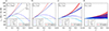 |
Fig. 3. LT precession frequency in LT and HT spacetimes. a) At the ISCO. b) Close to the ISCO. c) Close to the location of the maximum of the geodesic radial epicyclic frequency. d) At a larger radius, outside of the location of the maximum of the geodesic radial epicyclic frequency. The LT metric is shown in red. Lines in shades of blue correspond to the HT metric with varying q. The solid lines show the frequencies relevant to the test particle motion and slender tori. The colour-shaded regions indicate frequencies relevant to non-geodetic flows and cover all allowable torus thicknesses. The dotted line in panel a denotes the maximum frequency at the ISCO given by equation (14). |
5.1. Situation above ISCO
Situations at radii r3 : 1, r2 : 1, and r3 : 2, that are qualitatively similar to rISCO, are illustrated within panels b, c, and d of Figure 3. The test particle motion (and slender tori) frequencies are shown using solid lines, while the non-slender torus cases are indicated by shaded areas corresponding to tori of all thicknesses allowable according to the results of Matuszková et al. (2024b). While at r3 : 1 almost no quantitative difference exists between the test particle and fluid motion frequencies, at r2 : 1 the spread of frequencies given by the freedom in the torus thickness is clearly visible. Nevertheless, the behaviour of the fluid is qualitatively similar to the particle motion. At larger radii, represented by r3 : 2, the differences between the individual values of  are smaller but still apparent. In each panel of Figure 3, we also include the frequencies calculated in the LT spacetime. The frequency values predicted by monotonic functions associated with this spacetime are substantially higher than the maxima associated with the HT spacetime.
5.2. Maximum and averaged frequencies
Furthermore, we explore how the maximum possible observable precession frequency, νMAX, depends on the star’s angular momentum. For low values of j and  , it is simply the frequency at the ISCO, νMAX = νISCO. When there is a local radial maximum of the geodesic frequency, νmax0, which has a higher value than |νISCO|,
 (15)
(15)
otherwise
 (16)
(16)
which holds overall for any values of j and q. As can be seen in Figure 2, the pressure corrections to the geodesic frequency can be positive. In such situations, the maximum frequency associated with the fluid can exceed the value of the maximum geodesic frequency. In this case, however, the maximum absolute value at ISCO is always greater than that for non-geodesic motion. The overall dependence of νMAX on j is shown in the left panel of Figure 4.
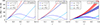 |
Fig. 4. Maximum and average value of the LT frequency. Left panel: Maximum of the frequency, νMAX, as a function of the angular momentum of the star. Middle panel: Frequency value averaged from rISCO to r2 : 1 as a function of the star’s angular momentum. Right panel: Frequency averaged from rISCO to r3 : 2 as a function of the star’s angular momentum. As in Figure 3, the red lines correspond to the LT metric, while the lines in shades of blue correspond to the HT metric and varying q. The shaded regions indicate the frequencies relevant to non-geodetic flows and cover the full range of allowable torus thicknesses. |
Finally, similar behaviour is also exhibited by the geodesic frequency averaged along the innermost parts of the disc, which is important when the observed LF QPOs are associated with fluid flows precessing as a rigid body (e.g. Ingram & Done 2011). Two examples of such frequencies are illustrated for the radii from ISCO to r2 : 1 (middle panel of Figure 4) and from ISCO to r3 : 2 (right panel of Figure 4). Within these panels, we also indicate the ranges relevant to the frequencies averaged in the same way but for the tori.
6. Surface
The investigation above does not take into account the restrictions imposed by the location of the compact object’s surface (e.g., Török et al. 2014; Pappas 2015; Urbancová et al. 2019). To illustrate these restrictions, we consider three different specific EoSs. The first two were chosen from the public CompOSE EoS library (CompOSE Core Team 2022) in such a way that they represent opposite margins of the overall region spanned by all COMPOSE EoSs in the mass-radius diagram. These are XMLSLZ (NL3; Xia et al. 2022) and VGBCMR (D1M; Viñas et al. 2021) EoSs. The third is the MIT bag EoS (Chodos et al. 1974), representing QSs, whereas we used the standard values B = 1014 g cm−3 for the bag constant and αc = 0.15 for strong interaction coupling constant.
In the top panels of Figure 5, we use the three EoS chosen above and plot the maximum LT precession frequency as a function of the NS angular momentum. The solid lines show the values when the star’s surface is below the ISCO, and the dashed lines show the values when it is above the ISCO. Furthermore, the plots allow us to determine whether the maximum frequency is reached at the edge of the relevant radial interval – the ISCO or NS surface – or above it. For practical purposes, it can also be useful to consider a sequence of stars with a constant non-rotating mass, M0, rather than a constant gravitational mass, M. This is illustrated in the bottom panels of Figure 5, which show a full analogy of the top panels, except that the fixed quantity is M0, while M increases from M = M0 towards higher values as j increases from j = 0. Figure 5 shows that, although stars with low masses extend above the ISCO, the effect of spin on the achieved value of the LT precession frequency is still similar for stars with high and low masses.
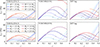 |
Fig. 5. Maximum LT precession frequency as a function of angular momentum of the star based on a specific EoS and a fixed gravitational mass, M (top panels), or a fixed non-rotating mass, M0 (bottom panels). Left panels: XMLSLZ(NL3) EoS. Middle panels: VGBCMR(D1M) EoS. Right panels: MIT bag EoS. The coloured solid lines show the values of νMAX when the star’s surface is below the ISCO, while the coloured dashed lines show the values of νMAX when the surface is above the ISCO. The circles on the individual lines enable us to determine the radius at which the maximum displayed frequency is reached. For values of j below that indicated by the black filled circle (or when there is no circle), the frequency corresponds to the edge of the relevant radial interval: the ISCO (solid lines) or the NS surface (dotted lines). For higher values of j, below the value indicated by the open circle, the frequency corresponds to the maximum above the edge. Above this value, it again corresponds to the ISCO for the solid lines and the NS surface for the dotted lines. The grey lines then indicate the value of the corresponding local geodesic maximum, νmax0. |
7. Discussion and conclusions
The works of Pappas (2012), Kluźniak & Rosińska (2013, 2014), Gondek-Rosińska et al. (2014), Pappas (2015), Tsang & Pappas (2016), and Matuszková et al. (2024a,b) have revealed the importance of the interplay between relativistic effects and effects already present in the Newtonian physics of oblate bodies. In the case of LT precession, this interplay takes place between the contributions of relativistic and classical precession, which have opposite directions, and this is crucial for our study utilising the HT spacetimes.
In contrast to the LT spacetime, which is linear in NS angular momentum, in the HT spacetime, the dependence of the frequency on j is not monotonic and exhibits maxima even for a moderately oblate NS. Figures 3–5, lead us to conclude that, within the innermost accretion region, the contribution of the relativistic precession to the overall precession ensures the growth of the total precession frequency only for a small interval of j. Afterwards, the frequency decreases due to the increasing contribution of the classical precession. Then, for higher j, the contribution of the classical precession drives the increase of the absolute frequency value, while the orientation of the resulting precession is reversed.
Consequently, within a sequence of NSs of equal mass and increasing rotational frequency, reaching moderate values of NS angular momentum, the precession frequencies can exhibit a sharp maximum at a particular value of the star’s rotational frequency. This conclusion, which holds for both geodesic and non-geodesic accretion flows, is relevant to the models of NS LF QPOs and implies that very different groups of accreting NSs, slow and fast rotators, can exhibit the same observable precession frequencies5. This may partially explain the previous observations, which revealed the lack of evidence for the expected correlation between the frequencies of QPOs and NS spin.
In the adopted framework, the units of measurement are chosen so that both the speed of light c and the gravitational constant G are equal to one (c = G = 1). Distances are measured in terms of the gravitational radius, rG = GM/c2, and the metric signature used is ( − , + , + , + ).
Although our initial focus in this section is on geodesic motion, the complete set of formulas presented in the associated Mathematica notebook is generally applicable to a non-geodesic fluid motion in thick accretion tori (Matuszková et al. 2024a). In the limit of zero torus thickness, this set reduces to formulae describing geodesic fluid motion or test particle motion. The geodesic case was considered in Urbancová et al. (2019). In their paper, which benefited from the introduction of  , the geodesic formulae originally derived by Abramowicz et al. (2003) were presented in a compact, physically self-consistent notation.
In the following, we adopt the convention that the negative sign of the frequency corresponds to the precession in the direction opposite to the direction of rotation.
Taking into account the thickness of the flow effectively implies a small quantitative correction to these frequencies when considering the innermost accretion region within a few gravitational radii.
Acknowledgments
We thank to the referee for valuable comments and suggestions. We acknowledge the Czech Science Foundation (GAČR) grants no. 21-06825X and 25-16928O, the MSK grant no. 04076/2024/RRC and the internal grant of the Silesian University in Opava no. SGS/25/2024.
References
- Abramowicz, M. A., & Kluźniak, W. 2001, A&A, 374, L19 [NASA ADS] [CrossRef] [EDP Sciences] [Google Scholar]
- Abramowicz, M. A., Almergren, G. J. E., Kluźniak, W., & Thampan, A. V. 2003, arXiv e-prints [arXiv:gr-qc/0312070] [Google Scholar]
- Altamirano, D., Ingram, A., van der Klis, M., et al. 2012, ApJ, 759, L20 [Google Scholar]
- Amsterdamski, P., Bulik, T., Gondek-Rosińska, D., & Kluźniak, W. 2002, A&A, 381, L21 [NASA ADS] [CrossRef] [EDP Sciences] [Google Scholar]
- Barret, D., & Vaughan, S. 2012, ApJ, 746, 131 [NASA ADS] [CrossRef] [Google Scholar]
- Barret, D., Kluźniak, W., Olive, J. F., Paltani, S., & Skinner, G. K. 2005a, MNRAS, 357, 1288 [Google Scholar]
- Barret, D., Olive, J.-F., & Miller, M. C. 2005b, MNRAS, 361, 855 [NASA ADS] [CrossRef] [Google Scholar]
- Barret, D., Olive, J.-F., & Miller, M. C. 2006, MNRAS, 370, 1140 [NASA ADS] [CrossRef] [Google Scholar]
- Belloni, T. M., & Motta, S. E. 2016, in Astrophysics of Black Holes: From Fundamental Aspects to Latest Developments, ed. C. Bambi, ASSL, 440, 61 [NASA ADS] [CrossRef] [Google Scholar]
- Belloni, T., Méndez, M., & Homan, J. 2007, MNRAS, 376, 1133 [Google Scholar]
- Blaes, O. M., Arras, P., & Fragile, P. C. 2006, MNRAS, 369, 1235 [NASA ADS] [CrossRef] [Google Scholar]
- Bollimpalli, D. A. 2022, MNRAS, 515, 6164 [Google Scholar]
- Bollimpalli, D. A., Fragile, P. C., Dewberry, J. W., & Kluźniak, W. 2024, MNRAS, 528, 1142 [Google Scholar]
- Čadež, A., Calvani, M., & Kostić, U. 2008, A&A, 487, 527 [NASA ADS] [CrossRef] [EDP Sciences] [Google Scholar]
- Chodos, A., Jaffe, R. L., Johnson, K., & Thorn, C. B. 1974, Phys. Rev. D, 10, 2599 [CrossRef] [Google Scholar]
- CompOSE Core Team (Typel, S., et al.) 2022, Eur. Phys. J. A, 58, 221 [NASA ADS] [CrossRef] [Google Scholar]
- de Avellar, M. G. B., Porth, O., Younsi, Z., & Rezzolla, L. 2018, MNRAS, 474, 3967 [NASA ADS] [CrossRef] [Google Scholar]
- du Buisson, L., Motta, S., & Fender, R. 2021, MNRAS, 502, 5472 [Google Scholar]
- Fragile, P. C. 2020, MNRAS, 491, 3245 [Google Scholar]
- Fragile, P. C., Straub, O., & Blaes, O. 2016, MNRAS, 461, 1356 [NASA ADS] [CrossRef] [Google Scholar]
- Gondek-Rosińska, D., Kluźniak, W., Stergioulas, N., & Wiśniewicz, M. 2014, Phys. Rev. D, 89, 104001 [CrossRef] [Google Scholar]
- Hartle, J. B. 1967, ApJ, 150, 1005 [NASA ADS] [CrossRef] [Google Scholar]
- Hartle, J. B., & Thorne, K. S. 1968, ApJ, 153, 807 [NASA ADS] [CrossRef] [Google Scholar]
- Ingram, A., & Done, C. 2010, MNRAS, 405, 2447 [NASA ADS] [Google Scholar]
- Ingram, A., & Done, C. 2011, MNRAS, 415, 2323 [NASA ADS] [CrossRef] [Google Scholar]
- Ingram, A., Done, C., & Fragile, P. C. 2009, MNRAS, 397, L101 [Google Scholar]
- Karas, V. 1999, ApJ, 526, 953 [Google Scholar]
- Kato, S. 2001, PASJ, 53, L37 [Google Scholar]
- Kluźniak, W., & Abramowicz, M. A. 2001, Acta Phys. Pol. B, 32, 3605 [Google Scholar]
- Kluźniak, W., & Rosińska, D. 2013, MNRAS, 434, 2825 [CrossRef] [Google Scholar]
- Kluźniak, W., & Rosińska, D. 2014, J. Phys. Conf. Ser., 496, 012016 [CrossRef] [Google Scholar]
- Kluźniak, W., Michelson, P., & Wagoner, R. V. 1990, ApJ, 358, 538 [Google Scholar]
- Kotrlová, A., Šrámková, E., Török, G., et al. 2020, A&A, 643, A31 [NASA ADS] [CrossRef] [EDP Sciences] [Google Scholar]
- Lattimer, J. M., & Prakash, M. 2001, ApJ, 550, 426 [NASA ADS] [CrossRef] [Google Scholar]
- Lense, J., & Thirring, H. 1918, Physikalische Zeitschrift, 19, 156 [NASA ADS] [Google Scholar]
- Lewin, W., & van der Klis, M. 2010, Compact Stellar X-ray Sources (Cambridge University Press) [Google Scholar]
- Lin, Y.-F., Boutelier, M., Barret, D., & Zhang, S.-N. 2011, ApJ, 726, 74 [Google Scholar]
- Lo, K.-W., & Lin, L.-M. 2011, ApJ, 728, 12 [NASA ADS] [CrossRef] [Google Scholar]
- Maselli, A., Pappas, G., Pani, P., et al. 2020, ApJ, 899, 139 [Google Scholar]
- Matuszková, M., Török, G., Klimovičová, K., et al. 2024a, A&A, 691, A168 [NASA ADS] [CrossRef] [EDP Sciences] [Google Scholar]
- Matuszková, M., Török, G., Lančová, D., et al. 2024b, A&A, 691, A167 [NASA ADS] [CrossRef] [EDP Sciences] [Google Scholar]
- Mauche, C. W. 2002, ApJ, 580, 423 [Google Scholar]
- Méndez, M. 2006, MNRAS, 371, 1925 [CrossRef] [Google Scholar]
- Middleton, M. J., Fragile, P. C., Ingram, A., & Roberts, T. P. 2019, MNRAS, 489, 282 [NASA ADS] [CrossRef] [Google Scholar]
- Mishra, B., Vincent, F. H., Manousakis, A., et al. 2017, MNRAS, 467, 4036 [CrossRef] [Google Scholar]
- Morsink, S. M., & Stella, L. 1999, ApJ, 513, 827 [NASA ADS] [CrossRef] [Google Scholar]
- Motta, S., Homan, J., Muñoz Darias, T., et al. 2012, MNRAS, 427, 595 [NASA ADS] [CrossRef] [Google Scholar]
- Motta, S. E., Belloni, T. M., Stella, L., Muñoz-Darias, T., & Fender, R. 2014, MNRAS, 437, 2554 [NASA ADS] [CrossRef] [Google Scholar]
- Motta, S. E., Belloni, T., Stella, L., et al. 2022, MNRAS, 517, 1469 [NASA ADS] [CrossRef] [Google Scholar]
- Pappas, G. 2012, MNRAS, 422, 2581 [Google Scholar]
- Pappas, G. 2015, MNRAS, 454, 4066 [NASA ADS] [CrossRef] [Google Scholar]
- Pappas, G., & Apostolatos, T. A. 2012, Phys. Rev. Lett., 108, 231104 [Google Scholar]
- Remillard, R. A., & McClintock, J. E. 2006, ARA&A, 44, 49 [Google Scholar]
- Rezzolla, L., Yoshida, S., Maccarone, T. J., & Zanotti, O. 2003a, MNRAS, 344, L37 [CrossRef] [Google Scholar]
- Rezzolla, L., Yoshida, S., & Zanotti, O. 2003b, MNRAS, 344, 978 [NASA ADS] [CrossRef] [Google Scholar]
- Stella, L., & Vietri, M. 1998, ApJ, 492, L59 [NASA ADS] [CrossRef] [Google Scholar]
- Stella, L., & Vietri, M. 1999, Phys. Rev. Lett., 82, 17 [NASA ADS] [CrossRef] [Google Scholar]
- Stella, L., Vietri, M., & Morsink, S. M. 1999, ApJ, 524, L63 [CrossRef] [Google Scholar]
- Strohmayer, T. E., Zhang, W., Swank, J. H., et al. 1996, ApJ, 469, L9 [Google Scholar]
- Stuchlík, Z., & Kološ, M. 2016a, ApJ, 825, 13 [CrossRef] [Google Scholar]
- Stuchlík, Z., & Kološ, M. 2016b, A&A, 586, A130 [NASA ADS] [CrossRef] [EDP Sciences] [Google Scholar]
- Török, G., Bakala, P., Stuchlík, Z., & Čech, P. 2008, Acta Astron., 58, 1 [Google Scholar]
- Török, G., Urbanec, M., Adámek, K., & Urbancová, G. 2014, A&A, 564, L5 [NASA ADS] [CrossRef] [EDP Sciences] [Google Scholar]
- Török, G., Goluchová, K., Horák, J., et al. 2016a, MNRAS, 457, L19 [CrossRef] [Google Scholar]
- Török, G., Goluchová, K., Urbanec, M., et al. 2016b, ApJ, 833, 273 [Google Scholar]
- Török, G., Goluchová, K., Šrámková, E., et al. 2018, MNRAS, 473, L136 [Google Scholar]
- Török, G., Kotrlová, A., Matuszková, M., et al. 2022, ApJ, 929, 28 [CrossRef] [Google Scholar]
- Tsang, D., & Pappas, G. 2016, ApJ, 818, L11 [NASA ADS] [CrossRef] [Google Scholar]
- Urbancová, G., Urbanec, M., Török, G., et al. 2019, ApJ, 877, 66 [CrossRef] [Google Scholar]
- van der Klis, M. 2006, in Compact Stellar X-ray Sources, eds. W. H. G. Lewin, & M. van der Klis (Cambridge University Press), 39, 39 [NASA ADS] [CrossRef] [Google Scholar]
- van Doesburgh, M., & van der Klis, M. 2017, MNRAS, 465, 3581 [Google Scholar]
- van Doesburgh, M., & van der Klis, M. 2019, MNRAS, 490, 5270 [Google Scholar]
- van Doesburgh, M., & van der Klis, M. 2020, MNRAS, 496, 5262 [Google Scholar]
- van Doesburgh, M., van der Klis, M., & Morsink, S. M. 2018, MNRAS, 479, 426 [Google Scholar]
- Viñas, X., Gonzalez-Boquera, C., Centelles, M., Mondal, C., & Robledo, L. M. 2021, Symmetry, 13, 1613 [Google Scholar]
- Wagoner, R. V., Silbergleit, A. S., & Ortega-Rodríguez, M. 2001, ApJ, 559, L25 [NASA ADS] [CrossRef] [Google Scholar]
- Xia, C.-J., Maruyama, T., Li, A., et al. 2022, Commun. Theor. Phys., 74, 095303 [Google Scholar]
- Zdunik, J. L., & Gourgoulhon, E. 2001, Phys. Rev. D, 63, 087501 [Google Scholar]
All Figures
|
Fig. 1. Frequencies of orbital motion around rotating NSs. a) NS spacetime approximated using the LT metric. b) Spacetime of extremely compact NSs approximated using the Kerr limit of the HT metric. c) Spacetime of highly oblate NSs approximated by the HT metric. The upper panels show the Keplerian and (axisymmetric) epicyclic frequencies. The bottom panels show the precession frequencies. The solid lines correspond to the frequencies of a test particle motion and slender tori. The colour-shaded regions indicate frequencies relevant to the non-geodesic flows of non-slender tori. The dashed lines in panel b indicate the frequencies of a test particle motion in the Kerr spacetime calculated using the appropriate coordinate transformation. |
| In the text | |
|
Fig. 2. Change in the orientation of the LT precession and behaviour of local frequency maxima shown for j = 0.35. As in Figure 1, the solid lines correspond to the frequencies of test particle motion and slender tori, while the shaded regions indicate the frequencies relevant to non-geodesic flows. The solid black circles indicate local maxima of the geodesic precession frequency, νmax0. |
| In the text | |
|
Fig. 3. LT precession frequency in LT and HT spacetimes. a) At the ISCO. b) Close to the ISCO. c) Close to the location of the maximum of the geodesic radial epicyclic frequency. d) At a larger radius, outside of the location of the maximum of the geodesic radial epicyclic frequency. The LT metric is shown in red. Lines in shades of blue correspond to the HT metric with varying q. The solid lines show the frequencies relevant to the test particle motion and slender tori. The colour-shaded regions indicate frequencies relevant to non-geodetic flows and cover all allowable torus thicknesses. The dotted line in panel a denotes the maximum frequency at the ISCO given by equation (14). |
| In the text | |
|
Fig. 4. Maximum and average value of the LT frequency. Left panel: Maximum of the frequency, νMAX, as a function of the angular momentum of the star. Middle panel: Frequency value averaged from rISCO to r2 : 1 as a function of the star’s angular momentum. Right panel: Frequency averaged from rISCO to r3 : 2 as a function of the star’s angular momentum. As in Figure 3, the red lines correspond to the LT metric, while the lines in shades of blue correspond to the HT metric and varying q. The shaded regions indicate the frequencies relevant to non-geodetic flows and cover the full range of allowable torus thicknesses. |
| In the text | |
|
Fig. 5. Maximum LT precession frequency as a function of angular momentum of the star based on a specific EoS and a fixed gravitational mass, M (top panels), or a fixed non-rotating mass, M0 (bottom panels). Left panels: XMLSLZ(NL3) EoS. Middle panels: VGBCMR(D1M) EoS. Right panels: MIT bag EoS. The coloured solid lines show the values of νMAX when the star’s surface is below the ISCO, while the coloured dashed lines show the values of νMAX when the surface is above the ISCO. The circles on the individual lines enable us to determine the radius at which the maximum displayed frequency is reached. For values of j below that indicated by the black filled circle (or when there is no circle), the frequency corresponds to the edge of the relevant radial interval: the ISCO (solid lines) or the NS surface (dotted lines). For higher values of j, below the value indicated by the open circle, the frequency corresponds to the maximum above the edge. Above this value, it again corresponds to the ISCO for the solid lines and the NS surface for the dotted lines. The grey lines then indicate the value of the corresponding local geodesic maximum, νmax0. |
| In the text | |
Current usage metrics show cumulative count of Article Views (full-text article views including HTML views, PDF and ePub downloads, according to the available data) and Abstracts Views on Vision4Press platform.
Data correspond to usage on the plateform after 2015. The current usage metrics is available 48-96 hours after online publication and is updated daily on week days.
Initial download of the metrics may take a while.