| Issue |
A&A
Volume 703, November 2025
|
|
|---|---|---|
| Article Number | L12 | |
| Number of page(s) | 9 | |
| Section | Letters to the Editor | |
| DOI | https://doi.org/10.1051/0004-6361/202554358 | |
| Published online | 13 November 2025 | |
Letter to the Editor
One-second variations in non-thermal X-ray source morphologies in an X-class solar flare
1
University College London, Mullard Space Science Labratory, Holmbury St Mary, Dorking, Surrey, RH5 6NT, UK
2
University of Applied Sciences and Arts Northwest Switzerland (FHNW), School of Computer Science, Bahnhofstrasse 6, Windisch, 5210, Switzerland
3
Istituto ricerche solari Aldo e Cele Daccò (IRSOL), Faculty of informatics, Università della Svizzera italiana, Locarno, Switzerland
4
Swiss Federal Institute of Technology in Zurich (ETHZ), Rämistrasse 1, 8001 Zürich, Switzerland
5
Astronomy & Astrophysics Section, School of Cosmic Physics, Dublin Institute for Advanced Studies, DIAS Dunsink Observatory, Dublin, D15 XR2R, Ireland
6
Space Sciences Laboratory, University of California, 7 Gauss Way, 94720 Berkeley, USA
⋆ Corresponding author: This email address is being protected from spambots. You need JavaScript enabled to view it.
Received:
3
March
2025
Accepted:
28
September
2025
Context. Modelling in recent decades suggests that electron acceleration in solar flares occurs on timescales of ≤1 s. Timeseries analyses of spatially integrated hard X-ray (HXR) emission from these electrons has shown similarly rapid variations. Further probing the acceleration process requires characterising the spatial and spectral evolution of the electrons with HXR imaging spectroscopy. However, this has not previously been available on such fast timescales.
Aims. We provide the first HXR spectroscopic imaging of accelerated electrons in a solar flare on timescales of 1 s.
Methods. We examined the evolution of non-thermal HXR source morphologies and their spatially averaged spectra in the solar flare SOL2024-05-20T05:14L171C109 (estimated-X16.5) with Solar Orbiter/STIX. The non-thermal component of this flare was one of the most intense ever observed, and STIX was the first solar HXR spectroscopic imager capable of 1 s (and sub-second) imaging. These observations are therefore the best so far for high-cadence non-thermal X-ray imaging spectroscopy.
Results. We observed physical changes in the non-thermal HXR source morphologies on timescales of 1 s, which is consistent with predictions for the acceleration process. The evolution of the spatially averaged electron spectral index was slower, however.
Conclusions. This may suggest a coherent driver between different acceleration events and/or pathways whose spectrum varies on timescales > 1 s. Alternatively, it may be an illusion of the spatial averaging in the spectral analysis. Either way, these results show that sub-second electron acceleration in solar flares can be associated with morphological dynamics on similar timescales. This highlights the importance of high spatial resolution sub-second HXR imaging spectroscopy for elucidating this process.
Key words: acceleration of particles / Sun: flares / Sun: particle emission / Sun: X-rays / gamma rays
© The Authors 2025
 Open Access article, published by EDP Sciences, under the terms of the Creative Commons Attribution License (https://creativecommons.org/licenses/by/4.0), which permits unrestricted use, distribution, and reproduction in any medium, provided the original work is properly cited.
This article is published in open access under the Subscribe to Open model. This email address is being protected from spambots. You need JavaScript enabled to view it. to support open access publication.
1. Introduction
The standard solar flare model (CSHKP; Carmichael 1964; Sturrock 1966; Hirayama 1974; Kopp & Pneuman 1976) posits that solar eruptive events are driven by energy that is released from highly stressed magnetic fields in the solar corona. One of the earliest observable consequences of this process is the non-thermal acceleration of electrons. These electrons emit hard X-ray (HXR) bremsstrahlung as they collide with ambient ions. Although these HXRs can be used to directly diagnose the accelerated electrons, because the bremsstrahlung spectrum directly reflects the velocity distribution of the emitting electrons, the mechanism(s) by which energy is transferred from the magnetic field to the electrons remains poorly understood. Recent models suggest that electrons can be accelerated on sub-second timescales (including, but not necessarily limited to, Fermi reflection in contracting magnetic islands; e.g. Drake et al. 2006, 2013; Arnold et al. 2021). This is consistent with time series analyses of spatially integrated HXR emission from flare-accelerated electrons, which have revealed spikes with durations from seconds to milliseconds (e.g. Kiplinger et al. 1983, 1984; Dennis 1985; Aschwanden et al. 1995; Knuth & Glesener 2020; Inglis & Hayes 2024). To fully constrain solar flare electron acceleration models, the spatial and spectral evolution of the electrons must be characterised via HXR imaging spectroscopy on timescales of ≤1 s. However, this has not previously been possible because of the limitations of past solar HXR spectroscopic imagers.
The first routine solar HXR imaging spectroscopy was provided by RHESSI (Reuven Ramaty High Energy Solar Spectroscopic Imager; Lin et al. 2002), which revolutionised our understanding of electron acceleration in solar flares. To bypass the challenges of directly focusing HXRs, RHESSI used an indirect imaging system. It decomposed spatial information into Fourier components, known as (complex) visibilities, from which images could be reconstructed via one of various algorithms (e.g. Piana et al. 2022). RHESSI measured its visibilities with rotation modulation collimators, which limited its fastest imaging cadence to half a spacecraft rotation (2 s; e.g. Qiu et al. 2012). Even this was rarely feasible, and RHESSI’s imaging cadence was typically limited to multiple rotational periods. This prevented RHESSI from imaging non-thermal sources on cadences relevant to the electron acceleration process.
A few studies have achieved cadences faster than 4 s when imaging non-thermal solar HXR sources. Sakao (1994) and Sakao et al. (1996) employed the Yohkoh Hard X-ray Telescope (HXT; Kosugi et al. 1991) to analyse the relative timing of sources in double HXR footpoint flares on a cadence of 0.5 s. They reported co-temporal HXR time evolution from the footpoints in six out of seven flares. Yohkoh/HXT did not provide true imaging spectroscopy, but was instead limited to four pre-defined broad energy bands between 20 and 100 keV. Thus, detailed spectra of the footpoints could not be determined. A similar study by Krucker & Lin (2002) used RHESSI to obtain spatially resolved spectra of individual HXR sources. In an attempt to overcome the limited imaging cadence of RHESSI, they produced images for overlapping 4 s intervals, offset by 1 s. Although changes from one image to the next were observed, fast, physically meaningful dynamics were likely masked by more dominant emission over each 4 s imaging intervals.
The Solar Orbiter Spectrometer/Telescope for Imaging X-rays (STIX; Krucker et al. 2020; Müller et al. 2013, 2020) is also an indirect Fourier imager, but does not employ rotation modulation collimators. Instead, its sub-collimators1 encode visibilities via moiré patterns that are produced by pairs of absorbing grids, each of which is sensitive to a different fixed orientation and angular scale (Massa et al. 2023). Its imaging cadence is therefore only limited by the time required to accumulate a statistically significant number of HXRs and the temporal cadence at which they are binned onboard. To date, this has been typically set to 0.5 s or 1 s depending on the telemetry budget of STIX, which varies with Solar Orbiter’s distance from Earth. STIX therefore has a greater ability to image the non-thermal electron distribution in sufficiently bright flares on timescales relevant to the acceleration process. In this Letter, we use STIX to provide the first HXR spectroscopic imaging of non-thermally accelerated electrons in a solar flare at a cadence of 1 s.
2. Observations and results
2.1. Observational configuration
We examined the SOL2024-05-20T05:14L171C109 solar flare (magenta dot and circle in Fig. 1). It had an estimated GOES-class of X16.5 (±1.8)2, which made it the largest flare of solar cycle 25 at the time of writing. It emanated from NOAA AR 13664 after it rotated onto the far side of the Sun relative to Earth (green dot Fig. 1). It was therefore visible to Solar Orbiter which was located at heliographic stonyhurst coordinates 170o longitude, 7o latitude, and 0.78 AU distance (blue dot, Fig. 1).
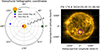 |
Fig. 1. Left: Approximate heliographic Stonyhurst coordinates of the Sun (yellow), Earth (green), Solar Orbiter (blue), and flare (magenta) at the time of the SOL2024-05-20T05:14L171C109 flare. (Not to scale.) Right: 174 Å image from the Extreme Ultraviolet Imager Full Sun Imager (EUI/FSI; Rochus et al. 2020) showing the perspective of Solar Orbiter and the approximate location of the flare (magneta circle). |
2.2. Spatially integrated spectral analysis
Figs. 2a and 2b show time series of raw STIX counts observed during the impulsive phase of the SOL2024-05-20T05:14L171C109 flare. The counts were summed over the 24 sub-collimators we used to image this flare (10a, 10b, 10c,…,3a, 3b and 3c). The 32–76 keV counts (blue solid) show two large non-thermal peaks, and the 15–18 keV counts (red dashed) show the more gradual evolution of the thermal plasma.
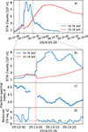 |
Fig. 2. Spectral evolution of the SOL2024-05-20T05:14L171C109 (estimated-X16.5) solar flare as a function of time (light arrival time at Solar Orbiter). All time bins are 1 s. a) and b) Thermal (red dashed; 15–18 keV) and non-thermal (blue solid; 32–76 keV) raw, uncorrected STIX counts summed over the 24 coarsest imaging sub-collimators (10a, 10b, 10c,…,3a, 3b and 3c). Two large non-thermal peaks are seen. The attenuator (inserted during the red time bin) absorbs few photons above 32 keV, but the increased detector live-time enabled by the reduction of lower energy counts caused those measured at 32–76 keV to increase. The grey vertical dashed lines in panel a) show the impulsive phase, which corresponds to the time axes of subsequent panels (and Fig. B.1). c) and d) Spatially averaged electron spectral index (panel c) and reduced χ2 statistics (panel d) obtained from fits to STIX spectra. The error bars represent the 1σ uncertainties. The response during the attenuator motion is uncertain, and the observations during the prior 3 seconds may have been compromised by increased pile-up. Consequently, we do not show fitting results for these times. |
Fits to the spatially integrated STIX spectra were performed with the OSPEX fitting software in the 32–70 keV spectral range. The fit model included a non-thermal thick-target distribution (f_thick2.pro) and an albedo component. The χ2 statistics (Fig. 2d) show that satisfactory fits were achieved. A thermal component was not required because its contribution was negligible in this spectral range during this time. (For justification, see Appendix A). The fits revealed that the non-thermal component of this flare was extremely bright. The predicted incident photon flux at 35 keV exceeded 600 photons s−1 keV−1 cm−2. By contrast, large flares typically have fluxes of < 10 photons s−1 keV−1 cm−2 (Battaglia et al. 2005), while the largest flares recorded by RHESSI had fluxes ∼200 photons s−1 keV−1 cm−2 (Xu et al. 2006; Krucker et al. 2011). This flare is therefore the best candidate to date for high-cadence non-thermal HXR imaging spectroscopy.
The same fits revealed that the electron spectral index (Fig. 2c) exhibited a smoothly varying soft-hard-soft behaviour on timescales of several seconds during both of the main non-thermal peaks. This seems to imply that the timescale of the electron acceleration process may in fact be > 1 s. We recall, however, that this represents the spatially averaged evolution.
2.3. Evidence of variations in non-thermal source morphologies on timescales of 1 s in STIX images
A different impression is revealed by the middle four columns of Fig. 3. They show MEM_GE image reconstructions (Massa et al. 2020) at a cadence of 1 s using the 24 coarsest sub-collimators of STIX (10a, 10b, 10c,…,3a, 3b and 3c) during the first large non-thermal peak (05:13:01–05:13:09). (For similar image reconstructions of the whole impulsive phase, see Fig. B.1.) To emphasise the evolution of the morphology between frames, we have normalised the colour maps so that they are consistent across all 1 s images, and have overlaid contours at 40% and 80% of the peak flux in each frame. The number of counts used in each image (top right corner of each frame) is greater than 10 000 (horizontal dashed line, left column)3. In contrast to the smoothly varying spatially integrated electron spectral index (Fig. 2c), the 1 s images show rapid morphological variations. The numbers and locations of sources change from one frame to the next, sometimes drastically. This suggests that substantial reconfiguration of the coronal magnetic field occurred on timescales ≤1 s. Sub-second variations may also be present, but not temporally resolved by these STIX observations.
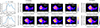 |
Fig. 3. STIX non-thermal images of the SOL2024-05-20T05:14L171C109 (estimated-X16.5) flare over the spectral range 32–76 keV and time interval 05:13:01–05:13:09 UT (light arrival time at Solar Orbiter). The images were constructed with the MEM_GE algorithm using the 24 coarsest imaging sub-collimators (10a, 10b, 10c,…,3a, 3b, 3c). Each row represents a sequential 4 s interval. Left column: Time series (blue) of the imaged counts, where each step represents 1 s. The grey region denotes the interval imaged in that row. The horizontal dashed line shows the 10 000 count level, and the red region denotes the time bin during which the attenuator was inserted. Middle 4 columns: Images with a 1 s integration time, progressing in time from left to right. The contours represent 40% and 80% of the peak flux in each image, and the colour table is scaled to be consistent across all 1 s images. The top right of each frame shows the number of counts used in each image. Right column: Images with a 4 s integration time corresponding to the same interval as the 1 s images in the same row. The contours and count labels are the same as in the middle rows, but the colour table is scaled across the 4 s images. It is not consistent with the 1 s images. |
The comparison of these images to those integrated over 4 s (right column) further emphasises the importance of high-cadence HXR imaging. (The colour map normalisation of these images is different to that of the 1 s images.) It shows that spatial dynamics can be hidden in HXR images that are integrated over the typical fastest RHESSI imaging cadence of 4 s. For example, the 1 s image at 05:13:01 is dominated by a northern source, followed a second later by a southern source. In the next second, the dominant source appears to have moved to the east, before growing more intense another second later. The corresponding 4 s image shows a circular source whose core is C-shaped and obscures the three distinct morphologies that dominated at different times. While sub-second variations in the spatially integrated HXR flare emission have long been established, this is the first time, to our knowledge, that morphological variations on similar timescales have been shown with HXR imaging spectroscopy.
2.4. Verifying the physical nature of the non-thermal source morphology dynamics via the STIX visibilities
Before drawing conclusions, however, we recall that interpreting the morphology of complex sources such as these can be ambiguous because the STIX sampling of the (u, v)-plane4 is limited. (Similar concerns apply to other indirect imagers.) In these scenarios, features caused by stochastic noise can be amplified by the image-reconstruction process and produce random variations between frames, especially when the morphologies are complex. To verify that the images in Fig. 3 contain physical evolution, we must therefore directly examine the visibilities that were used to produce them.
Complex visibilities have two key properties: amplitude and phase. They are measured by STIX as the amplitudes and peak locations of its moiré patterns (Massa et al. 2023). They mainly vary with two properties of the source(s): morphology, which can alter both amplitude and phase; and intensity, which alters all amplitudes by the same factor. To isolate variations associated with morphology, we normalised the amplitude of each visibility by the transmitted flux recorded by its detector. The resulting quantities, known as relative visibilities, are therefore independent of variations in the overall flux of the X-ray sources and only encode information on their morphology.
Fig. 4 shows the evolution of the relative visibilities over time (violet to red) for the same 1 s intervals shown in the middle four columns of Fig. 3. The relative visibilities are represented as single complex numbers (real components on the x-axes and imaginary components on the y-axes). Hence, the distance from the origin of each relative visibility represents its amplitude, and the angle it forms with the origin and the positive x-axis represents its phase. Each panel represents one of the six sub-collimators1 that varied most over this period (4c, 5b, 5c, 6b, 7b and 8b). (For the relative visibilities of all sub-collimators over this period, see Fig. C.1.) Second-to-second variations beyond 1 (error bars in Fig. 4) are evident at some time in all six sub-collimators. This is made clearer by the dotted grey circles centred on the origin, which provide a visual guide for changes in the amplitudes and phases of the relative visibilities. More compellingly, steady trends are seen, particularly in sub-collimators 8b, 7b, 6b and 4c. This strongly suggests that these variations are not random. This is further supported by the comparison in Appendix C (Fig. C.1) with thermal relative visibilities (15–18 keV) during the decay phase of the flare (05:14:42–05:14:50). At this time, the thermal source produced similarly good counting statistics and was expected to be much more morphologically stable. Consistent with this, the thermal relative visibilities are much more tightly clustered. This suggests that the variations in Fig. 4 are not caused by statistical fluctuations (see Appendix C for a further discussion.) Fig. 4 therefore demonstrates that these STIX observations capture physical evolution of the non-thermal source morphologies on timescales of 1 s.
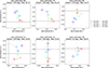 |
Fig. 4. The real (x axes) and imaginary parts (y axes) of STIX relative visibilities calculated over the period 2024-05-20 05:13:01–05:13:09 and spectral range 32–76 keV. Each panel corresponds to one of the six sub-collimators whose relative visibilities varied most over these ranges. The colours represent the evolution over time (violet to red) at a cadence of 1 s. The title of each panel gives the label, orientation, and angular resolution of the relevant sub-collimator. The error bars represent the 1σ uncertainties. The black dashed lines represent the x = 0 and y = 0 lines. The grey circles centred at the origin help to emphasise the variations in the amplitudes and phases of the relative visibilities. |
3. Discussion and conclusions
We have presented the first 1s-cadence HXR imaging spectroscopy of non-thermally accelerated electrons in a solar flare. Figs. 3 and 4 show strong evidence of physical morphological dynamics in the non-thermal HXR sources on timescales ≤1 s during the first large non-thermal peak. Similar rapid morphological dynamics may be present at earlier times (Appendix B and the first three rows of Fig. B.1), but the evidence is less conclusive because of the combination of the source complexity and the lower count rates. The morphology appears to change more slowly during the second large non-thermal peak, and the 4 s images seem sufficient to capture the evolution (lower rows, Fig. B.1). Although electrons continue to be accelerated, as evidenced by the non-thermal counts and electron spectral index (Figs. 2b and 2c), it appears that the magnetic pathways along which they propagate may be more restricted. This may be a result of reduced magnetic complexity in the reconnection region, or recently formed, more potential magnetic fields constraining the newly reconnected field lines. Alternatively, the spatial resolution and imaging dynamic range of STIX might be insufficient to identify emission from newly formed magnetic field lines amid the ongoing emission from those previously established. The slow evolution of the spatially averaged electron spectral index might suggest a common acceleration driver along different magnetic paths, whose spectrum varies on timescales > 1 s. This might also be an illusion of the spatial averaging in the spectral analysis, however. Either way, these results support models that predict solar electron acceleration on sub-second timescales, and show that this acceleration can be associated with spatial variations on similar timescales.
The minimum onboard binning employed by STIX during this flare (1 s) prevented us from identifying sub-second HXR fluctuations, and whether they correspond to similarly rapid spatial variations. To explore this, and to more rigorously test solar flare electron acceleration models, faster imaging spectroscopy with higher spatial resolution is needed. This is possible with STIX. During times of greater telemetry, the minimum onboard time binning is typically 0.5 s, and some campaigns have been run as fast as 0.3 s. During perihelia, Solar Orbiter reaches ∼0.3 AU from the Sun. This not only increases the HXR flux incident on STIX, but also facilitates 2.6 times greater spatial resolution than was possible for this flare. Furthermore, the STIX angular resolution would be increased by a factor of two if adequate calibration of its finest imaging grids could be provided in the future. This study therefore motivates dedicated fast-binning STIX campaigns when telemetry allows, especially when Solar Orbiter is closer to the Sun. Higher count rates and spatial resolution can then be achieved.
By emphasising the importance of sub-second imaging and spatially resolved spectroscopy, this study informs the design of future solar HXR spectroscopic imagers. Designs employing direct-focusing optics can achieve greater sensitivities than previous indirect imagers, enabling similar observations of dimmer, more frequent flares. They can also more easily separate spectra from different locations, which reduces the ambiguity in the spectral variability that is introduced by spatial averaging. The FOXSI-4 sounding rocket (Buitrago-Casas et al. 2021) has demonstrated the viability of this technology for solar flare observations, while FOXSI satellite concepts have previously been proposed (e.g. FOXSI-SMEX, Christe et al. 2023; FIERCE, Shih et al. 2020; SPARK, Reid et al. 2023). A mission concept like this remains a priority for making the next significant advances in understanding particle acceleration in solar flares.
Together, a pixellated spectroscopic detector and pair of absorbing grids that produce and measure a moiré pattern are known as a STIX (imaging) sub-collimator. As the pitch and orientation of the grids are fixed, each STIX imaging sub-collimator measures a single complex visibility with a fixed orientation on the plane of sky and angular scale.
Because this flare occurred on the backside of the Sun, and therefore was not visible to GOES, the GOES class was estimated from the counts in the STIX background detector (Stiefel et al. 2025).
10 000 counts is a “rule-of-thumb” minimum threshold for reducing imaging artefacts associated with low counting statistics when imaging multiple complex sources with STIX (Stiefel et al. 2023).
The (u, v)-plane is the 2D plane of angular frequencies that is sampled by indirect Fourier imagers. In the case of a STIX imaging sub-collimator, the pitch of its grids (as well as the separations between them and to the detector) makes it sensitive to a specific angular scale (Massa et al. 2023). This scale is inversely proportional to the distance of the sub-collimator’s (u, v)-coordinate from the origin. The u and v components of that coordinate depend on the orientation of the grids relative to the plane of sky. The greater the coverage of the (u, v)-plane (i.e. the more sub-collimators, for the STIX design), the more complex the sources that can be faithfully reconstructed from the observations.
Acknowledgments
Solar Orbiter is a space mission of international collaboration between ESA and NASA, operated by ESA. The STIX instrument is an international collaboration between Switzerland, Poland, France, Czech Republic, Germany, Austria, Ireland, and Italy. Preliminary analysis in this project was aided by tools provided by the STIX Data Center (Xiao et al. 2023), while more detailed analysis was supported in Python by the astropy (Astropy Collaboration 2013, 2018, 2022), sunpy (The SunPy Community 2020; Mumford et al. 2023), ndcube (Ryan et al. 2023a,b), xrayvision (pgabor et al. 2024), and stixpy (Maloney et al. 2024) packages, and their dependencies, and in IDL by the SolarSoftWare (SSW) distribution. Part of this work was supported by the German Deutsche Forschungsgemeinschaft, DFG project number Ts 17/2–1. PM is supported by the Swiss National Science Foundation in the framework of the project Robust Density Models for High Energy Physics and Solar Physics (rodem.ch), CRSII5_193716. L.A.H is supported through a Royal Society-Research Ireland University Research Fellowship.
References
- Arnold, H., Drake, J. F., Swisdak, M., et al. 2021, Phys. Rev. Lett., 126, 135101 [NASA ADS] [CrossRef] [Google Scholar]
- Aschwanden, M. J., Schwartz, R. A., & Alt, D. M. 1995, ApJ, 447, 923 [NASA ADS] [CrossRef] [Google Scholar]
- Astropy Collaboration (Robitaille, T. P., et al.) 2013, A&A, 558, A33 [NASA ADS] [CrossRef] [EDP Sciences] [Google Scholar]
- Astropy Collaboration (Price-Whelan, A. M., et al.) 2018, AJ, 156, 123 [Google Scholar]
- Astropy Collaboration (Price-Whelan, A. M., et al.) 2022, ApJ, 935, 167 [NASA ADS] [CrossRef] [Google Scholar]
- Battaglia, M., Grigis, P. C., & Benz, A. O. 2005, A&A, 439, 737 [NASA ADS] [CrossRef] [EDP Sciences] [Google Scholar]
- Buitrago-Casas, J. C., Vievering, J., Musset, S., et al. 2021, in UV, X-Ray, and Gamma-Ray Space Instrumentation for Astronomy XXII, ed. O. H. Siegmund, International Society for Optics and Photonics, SPIE, 11821, 118210L [Google Scholar]
- Carmichael, H. 1964, NASA SP, 50, 451 [Google Scholar]
- Christe, S., Alaoui, M., Allred, J., et al. 2023, BAAS, 55, 065 [NASA ADS] [Google Scholar]
- Dennis, B. R. 1985, Sol. Phys., 100, 465 [NASA ADS] [CrossRef] [Google Scholar]
- Drake, J. F., Swisdak, M., Che, H., & Shay, M. A. 2006, Nature, 443, 553 [Google Scholar]
- Drake, J. F., Swisdak, M., & Fermo, R. 2013, ApJ, 763, L5 [Google Scholar]
- Hirayama, T. 1974, Sol. Phys., 34, 323 [Google Scholar]
- Inglis, A. R., & Hayes, L. A. 2024, ApJ, 971, 29 [NASA ADS] [CrossRef] [Google Scholar]
- Kiplinger, A. L., Dennis, B. R., Frost, K. J., Orwig, L. E., & Emslie, A. G. 1983, ApJ, 265, L99 [Google Scholar]
- Kiplinger, A. L., Dennis, B. R., Frost, K. J., & Orwig, L. E. 1984, ApJ, 287, L105 [Google Scholar]
- Knuth, T., & Glesener, L. 2020, ApJ, 903, 63 [NASA ADS] [CrossRef] [Google Scholar]
- Kopp, R. A., & Pneuman, G. W. 1976, Sol. Phys., 50, 85 [Google Scholar]
- Kosugi, T., Makishima, K., Murakami, T., et al. 1991, Sol. Phys., 136, 17 [NASA ADS] [CrossRef] [Google Scholar]
- Krucker, S., & Lin, R. P. 2002, Sol. Phys., 210, 229 [Google Scholar]
- Krucker, S., Hudson, H. S., Jeffrey, N. L. S., et al. 2011, ApJ, 739, 96 [NASA ADS] [CrossRef] [Google Scholar]
- Krucker, S., Hurford, G. J., Grimm, O., et al. 2020, A&A, 642, A15 [NASA ADS] [CrossRef] [EDP Sciences] [Google Scholar]
- Lin, R. P., Dennis, B. R., Hurford, G. J., et al. 2002, Sol. Phys., 210, 3 [Google Scholar]
- Maloney, S., Clarke, B., Hayes, L., et al. 2024, https://doi.org/10.5281/zenodo.12752698 [Google Scholar]
- Massa, P., Schwartz, R., Tolbert, A. K., et al. 2020, ApJ, 894, 46 [NASA ADS] [CrossRef] [Google Scholar]
- Massa, P., Hurford, G. J., Volpara, A., et al. 2023, Sol. Phys., 298, 114 [NASA ADS] [CrossRef] [Google Scholar]
- Müller, D., Marsden, R. G., St. Cyr, O. C., Gilbert, H. R., & Solar Orbiter Team 2013, Sol. Phys., 285, 25 [CrossRef] [Google Scholar]
- Müller, D., St. Cyr, O. C., Zouganelis, I., et al. 2020, A&A, 642, A1 [Google Scholar]
- Mumford, S. J., Freij, N., Stansby, D., et al. 2023, https://doi.org/10.5281/zenodo.8384174 [Google Scholar]
- pgabor, Maloney, S., DanRyanIrish, et al. 2024, https://doi.org/10.5281/zenodo.14230355 [Google Scholar]
- Piana, M., Emslie, A., Massone, A. M., & Dennis, B. R. 2022, Hard X-ray Imaging of Solar Flares (Berlin: Springer) [Google Scholar]
- Qiu, J., Cheng, J. X., Hurford, G. J., Xu, Y., & Wang, H. 2012, A&A, 547, A72 [NASA ADS] [CrossRef] [EDP Sciences] [Google Scholar]
- Reid, H. A. S., Musset, S., Ryan, D. F., et al. 2023, Aerospace, 10, 1034 [NASA ADS] [CrossRef] [Google Scholar]
- Rochus, P., Auchère, F., Berghmans, D., et al. 2020, A&A, 642, A8 [NASA ADS] [CrossRef] [EDP Sciences] [Google Scholar]
- Ryan, D. F., Mumford, S., Barnes, W. T., et al. 2023a, ApJ, 956, 44 [Google Scholar]
- Ryan, D. F., Mumford, S., Sharma, Y., et al. 2023b, J. Open Source Softw., 8, 5296 [Google Scholar]
- Sakao, T. 1994, Ph.D. Thesis, University of Tokyo, Japan [Google Scholar]
- Sakao, T., Kosugi, T., Masuda, S., et al. 1996, Adv. Space Res., 17, 67 [NASA ADS] [CrossRef] [Google Scholar]
- Shih, A. Y., Glesener, L., Krucker, S., et al. 2020, https://doi.org/10.5281/zenodo.3674079 [Google Scholar]
- Stiefel, M. Z., Battaglia, A. F., Barczynski, K., et al. 2023, A&A, 670, A89 [NASA ADS] [CrossRef] [EDP Sciences] [Google Scholar]
- Stiefel, M. Z., Kuhar, M., Limousin, O., et al. 2025, A&A, 694, A138 [NASA ADS] [CrossRef] [EDP Sciences] [Google Scholar]
- Sturrock, P. A. 1966, Nature, 211, 695 [Google Scholar]
- The SunPy Community (Barnes, W. T., et al.) 2020, ApJ, 890, 68 [Google Scholar]
- Xiao, H., Maloney, S., Krucker, S., et al. 2023, A&A, 673, A142 [NASA ADS] [CrossRef] [EDP Sciences] [Google Scholar]
- Xu, Y., Cao, W., Liu, C., et al. 2006, ApJ, 641, 1210 [NASA ADS] [CrossRef] [Google Scholar]
Appendix A: Sample spectral fit
To help justify the fitting process outlined in Sect. 2, and our assertion that the images in Fig. 3 are predominantly non-thermal, we show an example STIX spectrum in Fig. A.1. It has been integrated over 2 s around the second major peak in the non-thermal emission (05:13:21 – 05:13:23; light arrival time at Solar Orbiter). The second peak was chosen as a worst case scenario as there has been more time since the start of the flare for the thermal plasma to evolve and dominate. The iterative fitting technique of Stiefel et al. (2025) was used to fit both the summed count spectrum from the imaging detectors (left panel, Fig. A.1) and the background (BKG) detector (right panel, Fig. A.1). Both spectra were fit with a model including two isothermal components combined with a thick-target non-thermal and an albedo component. Note that while the parameters of the spectral components are the same for both spectra, their shapes appear to differ. This is because the attenuator was inserted for the imaging detectors at this time, while an attenuator is never used for the BKG detector. (For the spectral response of the attenuator, see Fig. 3 of Krucker et al. 2020.) These different attenuation strategies enable the BKG spectrum to constrain the low-energy regime (6 – 28 keV), which is particularly beneficial for the thermal components. Meanwhile, the imaging detectors’ better count statistics at higher energies (> 12 keV), better constrain the non-thermal component. The residuals of the fits are generally satisfactory, with the largest deviation around the tungsten K-edge at 69.5 keV. We attribute this to inaccuracies in the current imaging grid calibration, which will be improved in the future.
The spectra show that at 32 keV, the non-thermal component, together with the albedo, make up 99% of the total counts. This percentage increases for higher energies. Examination of spectra at other times (not shown) suggests that the direct and albedo non-thermal contribution to the 32 – 76 keV spectral range remains stable within a couple percent during the entire period examined by in Figs. 3, 4 and B.1, and left three columns of Fig. C.1. This justifies the spectral fitting method used in Sect. 2 to derive the electron spectral index (Fig. 2c). It also supports our assertion that the changes seen in Figs. 3 and 4 are due to the spatial distribution of non-thermally accelerated electrons, and not an increasing presence of chromospherically evaporated thermal plasma.
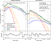 |
Fig. A.1. Observed STIX spectra (black) integrated over 2 s around the second large non-thermal peak of the SOL2024-05-20T05:14L171C109 (estimated-X16.5) flare (05:13:21 – 05:13:23). The summed spectra from the 24 coarsest angular resolution imaging sub-collimators (left) and pixels 2 and 5 of the background detector (BKG; right) are shown. The best fit (green) is derived by applying an iterative fitting method (Stiefel et al. 2025) to both spectra with a model including thermal (red), superhot thermal (yellow), non-thermal thick-target (blue), and albedo (grey) components. The fitted spectral ranges (12 – 100 keV for imaging detectors; 6 – 28 keV for the BKG detector) are denoted by the vertical dotted lines. The lower panels show the fit residuals, whose calculation included a 5% systematic error. The best-fit model parameters are given in the top right, along with their uncertainties. |
Appendix B: Imaging the impulsive phase
Fig. B.1 represents an extension of Fig. 3 to the whole impulsive phase of the SOL2024-05-20T05:14L171C109 (estimated-X16.5-class) flare (05:12:48 – 05:13:29 UT, light arrival time at Solar Orbiter). The structure, symbols, colour maps, contours, spectral range, imaging cadences and imaging sub-collimators used are the same as in Fig. 3. In fact, Fig. 3 itself can be seen as the 4th and 5th rows of Fig. B.1. Rapid morphological variations can be seen at the start of the impulsive phase (first three rows) in the 1 s images (middle four columns), which are not captured by the 4 s images (right column). However, the count rates of the 1 s images are a factor of 2 – 3 lower than those presented in Fig. 3. It is therefore less certain than at subsequent times whether these variations are physical. By contrast, the count rates during the second non-thermal peak (rows 6 – 9) are comparable to those in Fig. 3. However, the morphology appears to change much more slowly, and the 4 s images seem sufficient to capture many of the dynamics.
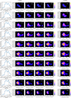 |
Fig. B.1. STIX MEM_GE non-thermal imaging results over the spectral range 32 – 76 keV during the rise phase of the SOL2024-05-20T05:14L171C109 (estimated-X16.5) flare. Left column: 32 – 76 keV integrated lightcurves. Grey regions show the 4 s interval imaged in each row. The red region shows the 1 s time bin encompassing the attenuator motion, during which images were not produced. Middle 4 columns: 1 s-integration images progressing in time from left to right, and then downward through each row. White/black lines show 40% and 80% contours relative to the peak intensity in each image. The colour table is scaled to be consistent across all 1 s images. The number of counts used for each image is given in the top right corner of each frame. Right column: 4 s-integration images corresponding to the same interval as the 1 s images in the same row. The contours and count labels are as in the middle rows, but the colour table is scaled across all 4 s images, and is not consistent with the 1 s images. Note that some rows show morphological changes on ≤1 s timescales that are not captured by the 4 s images. |
Appendix C: Verifying morphological changes via observed relative visibilities
The left three columns of Fig. C.1 show an extension of Fig. 4 to all the STIX imaging sub-collimators1 used in this study. It considers the same 8 consecutive 1 s integration times examined in Figs. 3 and 4. The colour coding, symbols, dashed lines and dotted circles all have the same meanings as Fig. 4, and each panel represents visibilities from a different sub-collimator. The examined time range presents large counting statistics (∼60K to ∼90K recorded counts), which helps to minimise variations in the visibilities due to statistical fluctuations.
As shown in Fig. 4, the non-thermal relative visibilities measured by sub-collimators 8b, 7b, 6b, and 4c show clear 1 s variations. Less statistically significant, but still suggestive, changes are seen in sub-collimators 10b, 5b, 5c. Although the changes from second to second are only on the order of 1 – 2σ, and therefore of limited statistical significance by themselves, their overall evolution is consistent and strongly suggests that morphological changes in the non-thermal X-ray emission do occur on at least 1 s timescales. The absence of statistically significant changes in other sub-collimators does not undermine this assertion, but simply implies that the morphological changes are asymmetric. The variations highlight the importance of the ≤1 s imaging cadences achievable with STIX compared to RHESSI’s typical best imaging cadence of 4 s. With only a 4 s cadence, we have only two data points per plot, and can not track the evolution of the source morphology. We are hence blind to potential relationships between morphological changes and the timescale of electron acceleration.
To further justify our assertion that the changes in the non-thermal relative visibilities are physical and not due to statistical fluctuations, we compare them with the right three columns of Fig. C.1. These show relative visibilities calculated in the thermal range (15 – 18 keV) for a different 8 s period during the flare’s decay phase (05:14:42 – 05:14:50). This time range was chosen because the thermal morphology was expected to be fairly stable and corresponds to similar counting statistics (∼70K counts per second) to the non-thermal case. Note that the relative visibilities form a more compact cluster for all sub-collimators, with the exceptions of sub-collimators 10c, 9c, and 8c. Although these sub-collimators present a larger scatter, they do not show a consistent trend over time. This demonstrates that a morphologically stable source would be expected to present much tighter spreads and less pronounced trends in relative visibilities than seen in the non-thermal columns. This further supports our conclusion that STIX is capturing real morphological changes in the non-thermal sources on a timescale on or approaching that of the electron acceleration process.
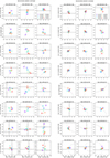 |
Fig. C.1. Scatter plots of the real and the imaginary parts of the relative visibilities for each sub-collimator for the non-thermal (left 3 columns; 32 – 76 keV; 05:13:01 – 05:13:09 UT) and thermal (right 3 columns; 15 – 18 keV; 05:14:42 – 05:14:50 UT) emission. (Times represent light arrival time at Solar Orbiter.) Each point corresponds to a 1s integration time and is colour-coded in time from violet to red. Error bars represent 1σ uncertainties. The black dashed lines represent the x = 0 and y = 0 lines, while the grey circles centred at the origin help highlight changes in the relative visibilities’ amplitudes and phases. |
All Figures
|
Fig. 1. Left: Approximate heliographic Stonyhurst coordinates of the Sun (yellow), Earth (green), Solar Orbiter (blue), and flare (magenta) at the time of the SOL2024-05-20T05:14L171C109 flare. (Not to scale.) Right: 174 Å image from the Extreme Ultraviolet Imager Full Sun Imager (EUI/FSI; Rochus et al. 2020) showing the perspective of Solar Orbiter and the approximate location of the flare (magneta circle). |
| In the text | |
|
Fig. 2. Spectral evolution of the SOL2024-05-20T05:14L171C109 (estimated-X16.5) solar flare as a function of time (light arrival time at Solar Orbiter). All time bins are 1 s. a) and b) Thermal (red dashed; 15–18 keV) and non-thermal (blue solid; 32–76 keV) raw, uncorrected STIX counts summed over the 24 coarsest imaging sub-collimators (10a, 10b, 10c,…,3a, 3b and 3c). Two large non-thermal peaks are seen. The attenuator (inserted during the red time bin) absorbs few photons above 32 keV, but the increased detector live-time enabled by the reduction of lower energy counts caused those measured at 32–76 keV to increase. The grey vertical dashed lines in panel a) show the impulsive phase, which corresponds to the time axes of subsequent panels (and Fig. B.1). c) and d) Spatially averaged electron spectral index (panel c) and reduced χ2 statistics (panel d) obtained from fits to STIX spectra. The error bars represent the 1σ uncertainties. The response during the attenuator motion is uncertain, and the observations during the prior 3 seconds may have been compromised by increased pile-up. Consequently, we do not show fitting results for these times. |
| In the text | |
|
Fig. 3. STIX non-thermal images of the SOL2024-05-20T05:14L171C109 (estimated-X16.5) flare over the spectral range 32–76 keV and time interval 05:13:01–05:13:09 UT (light arrival time at Solar Orbiter). The images were constructed with the MEM_GE algorithm using the 24 coarsest imaging sub-collimators (10a, 10b, 10c,…,3a, 3b, 3c). Each row represents a sequential 4 s interval. Left column: Time series (blue) of the imaged counts, where each step represents 1 s. The grey region denotes the interval imaged in that row. The horizontal dashed line shows the 10 000 count level, and the red region denotes the time bin during which the attenuator was inserted. Middle 4 columns: Images with a 1 s integration time, progressing in time from left to right. The contours represent 40% and 80% of the peak flux in each image, and the colour table is scaled to be consistent across all 1 s images. The top right of each frame shows the number of counts used in each image. Right column: Images with a 4 s integration time corresponding to the same interval as the 1 s images in the same row. The contours and count labels are the same as in the middle rows, but the colour table is scaled across the 4 s images. It is not consistent with the 1 s images. |
| In the text | |
|
Fig. 4. The real (x axes) and imaginary parts (y axes) of STIX relative visibilities calculated over the period 2024-05-20 05:13:01–05:13:09 and spectral range 32–76 keV. Each panel corresponds to one of the six sub-collimators whose relative visibilities varied most over these ranges. The colours represent the evolution over time (violet to red) at a cadence of 1 s. The title of each panel gives the label, orientation, and angular resolution of the relevant sub-collimator. The error bars represent the 1σ uncertainties. The black dashed lines represent the x = 0 and y = 0 lines. The grey circles centred at the origin help to emphasise the variations in the amplitudes and phases of the relative visibilities. |
| In the text | |
|
Fig. A.1. Observed STIX spectra (black) integrated over 2 s around the second large non-thermal peak of the SOL2024-05-20T05:14L171C109 (estimated-X16.5) flare (05:13:21 – 05:13:23). The summed spectra from the 24 coarsest angular resolution imaging sub-collimators (left) and pixels 2 and 5 of the background detector (BKG; right) are shown. The best fit (green) is derived by applying an iterative fitting method (Stiefel et al. 2025) to both spectra with a model including thermal (red), superhot thermal (yellow), non-thermal thick-target (blue), and albedo (grey) components. The fitted spectral ranges (12 – 100 keV for imaging detectors; 6 – 28 keV for the BKG detector) are denoted by the vertical dotted lines. The lower panels show the fit residuals, whose calculation included a 5% systematic error. The best-fit model parameters are given in the top right, along with their uncertainties. |
| In the text | |
|
Fig. B.1. STIX MEM_GE non-thermal imaging results over the spectral range 32 – 76 keV during the rise phase of the SOL2024-05-20T05:14L171C109 (estimated-X16.5) flare. Left column: 32 – 76 keV integrated lightcurves. Grey regions show the 4 s interval imaged in each row. The red region shows the 1 s time bin encompassing the attenuator motion, during which images were not produced. Middle 4 columns: 1 s-integration images progressing in time from left to right, and then downward through each row. White/black lines show 40% and 80% contours relative to the peak intensity in each image. The colour table is scaled to be consistent across all 1 s images. The number of counts used for each image is given in the top right corner of each frame. Right column: 4 s-integration images corresponding to the same interval as the 1 s images in the same row. The contours and count labels are as in the middle rows, but the colour table is scaled across all 4 s images, and is not consistent with the 1 s images. Note that some rows show morphological changes on ≤1 s timescales that are not captured by the 4 s images. |
| In the text | |
|
Fig. C.1. Scatter plots of the real and the imaginary parts of the relative visibilities for each sub-collimator for the non-thermal (left 3 columns; 32 – 76 keV; 05:13:01 – 05:13:09 UT) and thermal (right 3 columns; 15 – 18 keV; 05:14:42 – 05:14:50 UT) emission. (Times represent light arrival time at Solar Orbiter.) Each point corresponds to a 1s integration time and is colour-coded in time from violet to red. Error bars represent 1σ uncertainties. The black dashed lines represent the x = 0 and y = 0 lines, while the grey circles centred at the origin help highlight changes in the relative visibilities’ amplitudes and phases. |
| In the text | |
Current usage metrics show cumulative count of Article Views (full-text article views including HTML views, PDF and ePub downloads, according to the available data) and Abstracts Views on Vision4Press platform.
Data correspond to usage on the plateform after 2015. The current usage metrics is available 48-96 hours after online publication and is updated daily on week days.
Initial download of the metrics may take a while.