| Issue |
A&A
Volume 703, November 2025
|
|
|---|---|---|
| Article Number | A54 | |
| Number of page(s) | 16 | |
| Section | Numerical methods and codes | |
| DOI | https://doi.org/10.1051/0004-6361/202554494 | |
| Published online | 04 November 2025 | |
WIggle Corrector Kit for NIRSpEc Data: WICKED
1
Max Planck Institute for Astronomy,
Königstuhl 17,
69117
Heidelberg,
Germany
2
Department of Physics and Astronomy, University of Utah
115 South 1400 East,
Salt Lake City,
UT
84112,
USA
3
European Space Agency, Space Telescope Science Institute,
Baltimore,
MD,
USA
4
Department of Astronomy & Astrophysics and Institute for Gravitation and the Cosmos, The Pennsylvania State University,
525 Davey Lab,
University Park,
PA
16802,
USA
5
Department of Astrophysical Sciences, Princeton University,
4 Ivy Lane,
Princeton,
NJ
08544,
USA
6
Department of Astronomy, University of Michigan,
1085 S. University Avenue,
Ann Arbor,
MI
48109,
USA
7
Kavli Institute for Astronomy and Astrophysics, Peking University,
Beijing
100871,
China
8
Department of Astronomy, School of Physics, Peking University,
Beijing
100871,
China
9
George P. and Cynthia Woods Mitchell Institute for Fundamental Physics and Astronomy and Department of Physics and Astronomy, Texas A&M University,
College Station,
TX
77843,
USA
10
European Space Research and Technology Centre,
Keplerlaan 1,
2200 AG
Noordwijk,
The Netherlands
★ Corresponding author: This email address is being protected from spambots. You need JavaScript enabled to view it.
Received:
12
March
2025
Accepted:
1
September
2025
Abstract
Context. The point spread function of the integral field unit (IFU) mode of the Near-Infrared Spectrograph (NIRSpec) detector of JWST is undersampled. The resampling of the spectra into a 3D data cube creates resampling noise seen as low-frequency sinusoidal-like artifacts, or “wiggles.” These artifacts in the data are not corrected in the JWST data pipeline and significantly impact the science that can be achieved at a single-pixel level.
Aims. Here we present the tool “WIggle Corrector Kit for NIRSpEc Data” (WICKED) designed to remove these artifacts. While fully characterizing wiggles requires forward modeling of the instrument response, WICKED offers a faster and computationally efficient alternative using an empirical correction.
Methods. WICKED uses the fast Fourier transform algorithm to identify wiggle-affected spaxels across the (IFU) data cube. Spectra are modeled with a mix of integrated aperture and annular templates, a power law, and a second-degree polynomial, thus avoiding the high-degree polynomials that distort spectral features. Our correction works across all medium- and high-resolution NIRSpec gratings: F070LP, F100LP, F170LP, and F290LP.
Results. The overall spectral shape recovered by WICKED is up to 3.5 times better compared to uncorrected spectra. It recovers the equivalent width of absorption lines within 5% of the true value, which is also roughly three times better than the uncorrected spectra. WICKED7 significantly improves kinematic measurements, recovering the line-of-sight velocity (LOSV) within 1% of the true value – more than 100 times better than uncorrected spectra at S/N ~ 40. As a case study, we applied WICKED to G235H/F170LP IFU data of the elliptical galaxy NGC 5128, finding good agreement with previous studies. In wiggle-affected regions, the uncorrected spectrum showed a stellar LOSV and velocity dispersion differences ~17 times and ~36 times larger than the estimated uncertainties, respectively, compared to the WICKED-cleaned spectrum.
Conclusions. Wiggles in NIRSpec IFU data can significantly distort the overall spectral shape and bias line measurements and kinematics to values larger than the expected uncertainties for uncorrected spectra. WICKED is a robust, user-friendly solution for mitigating wiggles in NIRSpec data that enables precise single-spaxel studies and enhances JWST’s potential for groundbreaking discoveries in galaxy kinematics and early Universe studies.
Key words: methods: data analysis / galaxies: general / galaxies: kinematics and dynamics / galaxies: nuclei
© The Authors 2025
 Open Access article, published by EDP Sciences, under the terms of the Creative Commons Attribution License (https://creativecommons.org/licenses/by/4.0), which permits unrestricted use, distribution, and reproduction in any medium, provided the original work is properly cited.
This article is published in open access under the Subscribe to Open model.
Open Access funding provided by Max Planck Society.
1 Introduction
In only three years since the launch of the James Webb Space Telescope (JWST) (Gardner et al. 2023), its unprecedented gain in sensitivity in the near- and mid-infrared has already revolutionized the study of the early Universe. JWST is equipped with two integral field unit (IFU) spectrographs, NIRSpec (Jakobsen et al. 2022) and MIRI (Wright et al. 2023), that provide spectral information across the field of view and enable spatially resolved studies and chemical abundances. However, both IFU units of JWST are spatially undersampled, staying below the desired Nyquist sampling at any wavelength, which creates significant resampling noise modulations (Smith et al. 2007; Law et al. 2023). NIRSpec, in particular, is the IFU mode most affected by undersampling of the point spread function (PSF), with a full width half maximum (FWHM) at 3 microns equal to its pixel size of 0.1″ (Ruffio et al. 2024). As a result, prominent low-frequency (5–60 [1/µm]) PSF artifacts commonly referred to as “wiggles” are present in many NIRSpec IFU observations, and currently there is no correction for them in the JWST pipeline. With JWST breaking records for proposal submissions and NIRSpec being the most requested instrument1, addressing these artifacts has become a priority. The ideal approach for correcting these artifacts would involve forward modeling of mock data to accurately simulate the NIRSpec instrument. These simulations could then be compared to observations to identify and subtract the wiggles. Forward modeling has been done for the NIRSpec multi-object spectroscopic (MOS) mode for a sample of high-redshift galaxies in the JWST Advanced Deep Extragalactic Survey (JADES) (de Graaff et al. 2024), but it is currently unavailable for the IFU mode. Forward modeling is computationally expensive and challenging to implement due to the complexity of the JWST NIRSpec PSF, with de Graaff et al. (2024) and Ruffio et al. (2024) being the only examples available so far. Additionally, generating accurate simulations to account for the unique characteristic of every dataset is also a challenge. Consequently, empirical, post-facto correction methods offer a more practical and efficient alternative. Previous studies using NIRSpec IFU data have often relied on spatially binning the data to apertures equal to or larger than the PSF (e.g., Bianchin et al. 2024), particularly for studies of point sources where these artifacts are more pronounced. Others have addressed the issue by simply ignoring and masking out the affected spaxels (e.g., Donnan et al. 2024). Two groups have attempted to develop fitting routines to remove these wiggles. One routine uses an integrated spectrum template (Perna et al. 2023), and the other uses a single power law (Doan et al. 2025) to model the spectrum across the IFU’s field of view. The wiggles are then identified as the difference between the data and the model. The wiggles in the spectrum display a sinusoidal pattern with varying amplitude and frequency across the wavelength range. While the amplitude and phase of the wiggles for each spaxel in the IFU are different, Perna et al. (2023) found that the wiggle frequencies are not random but correlate with wavelength. This correlation appears consistent across all spaxels in the field of view and can be used to model the wiggles as a series of sine functions with a frequency determined by the wavelength. The method by Perna et al. (2023) has demonstrated the feasibility of removing wiggles using an empirical post-facto approach, and it is currently the best available tool to remove these artifacts from NIRSpec IFU data. However, it has two main limitations. (1) In certain cases it can significantly alter the spectral shape of the continuum, and (2) it offers a more limited method for flagging affected spaxels across the field of view based only on a signal-to-noise threshold of the central compact source.
To address these challenges, we have developed WICKED (Wiggle Corrector Kit for NIRSpec Data), a user-friendly PYTHON class designed to remove resampling noise artifacts, or wiggles, from NIRSpec IFU data for all medium- and high-resolution gratings: F070LP, F100LP, F170LP, and F290LP. WICKED applies the fast Fourier transform algorithm to identify and flag affected spaxels while avoiding the high-degree polynomials used by Perna et al. (2023) to model the continuum of the spectrum, which affects the integrity of the data.
This paper is organized as follows: In Section 2.1 we describe the data reduction for the NIRSpec IFU data of four stars as well as for the elliptical galaxy NGC 5128 (also known as Centaurus A) used as test cases. In Section 3 we give a detailed description of the WICKED algorithm. Section 4 shows the results of several tests developed to quantify WICKED’s performance. Section 5 shows the results of the stellar and gas kinematics for the NIRSpec F170LP IFU data of NGC 5128, corrected for wiggles using WICKED. Finally, in Section 6 we present a summary of the methodology and the results for WICKED before discussing the findings for the kinematics of NGC 5128.
2 Data
In this work, we used JWST NIRSpec IFU archival observations of the four stars 2MASS J17571324+6703409, 2MASS-J153950773404566, BD+04-3653, GSPC P330-E and the nucleus of NGC 5128. The high resolution IFU mode of NIR-Spec can obtain spectra in the wavelength range of 0.6–5.3 µm for a 3.1″ × 3.2″ field of view and a spectral resolution of R ≈ 2700 (Böker et al. 2022). We used the stellar spectra of stars for testing the performance of WICKED, and the nucleus of NGC 5128 as a practical example of the science that can be achieved after correcting for wiggles in the NIR-Spec IFU spectra. The observations for the A-type star 2MASS J17571324+6703409 (hereafter “J17571324”) are part of the Cycle 2 program PID3399 (PI: Marshall Perrin) taken with a 16-dither pattern in the high-resolution mode G235H/F170LP with a total integration time of 3968 s. observations for the M-type star 2MASS-J15395077-3404566 (hereafter: “J15395077”) and BD+04-3653 were taken for Cycle 1 program PID1364 (PI: Misty C. Bentz) using of four-dither pattern with a total integration time of ~171 s in the high resolution G235H/F170LP configuration. The observations of GSPC P330-E (hereafter: P330-E) are part of the Cycle 1 program PID1538 (PI: Karl D. Gordon) also taken with a four-dither pattern and a total integration time of 175 s in the medium resolution G235M/F170LP configuration. Finally, observations of the nucleus of NGC 5128 were obtained for a GTO program PID1269 (PI: Nora Luetzgendorf) using a four-point dither pattern with a total integration time of 933.7 s per configuration in the high-resolution modes G235H/F170LP and G395H/F290LP, with one leakcal image taken per configuration with a total integration time of 233.5 s.
2.1 NIRSpec IFU data reduction
The NIRSpec IFU data were reduced using the JWST data pipeline2 version 1.12.5 and context file “jwst_1256.pmap” (Bushouse et al. 2024). The data reduction was identical for J17571324, J15395077, BD+04-3653, P330-E, and NGC 5128 except that for NGC 5128, a leakcal image was used. We started the reduction by running the Detector1Pipeline module of the JWST pipeline on all raw uncal.fits files. We used the patch SNOWBLIND (Davies 2024) during Detector1Pipeline to correct for large cosmic ray hits. For this, we saved the “jump.fits” files during the DETECTOR1PIPELINE and passed them to SNOWBLIND which detected and masked pixels affected by cosmic-ray hits. The clean “jump.fits” are passed again to Detector1Pipeline to run the remaining steps until obtaining a “rate.fits” file. The count-rate files were then processed using the Calwebb_spec2 module with default parameters, but using the NSClean (Rauscher 2024) step (now incorporated into the JWST pipeline) to correct for correlated noise. Finally, the resulting “cal.fits” files were resampled and co-added using the “drizzle” weighting into a cube using the Calwebb_spec3 with a spaxel size of 0.″ 1 and the instrument alignment.
All the resulting cubes present substantial sinusoidal patterns in their spectra at the single spaxel level (see left panel in Figure A.1), due to resampling noise caused by the under-sampling of the PSF (Law et al. 2023). The frequency of the wiggles is related to the change in tilt between the trace of the spectral dispersion and the detector grid (Law et al. 2023). This creates a characteristic frequency for the wiggles in the medium and high resolution configurations independently of the source, as shown in the right panel of Figure A.1. Wiggles are particularly noticeable near the cores of compact sources such as stars, active galactic nuclei (AGN), and quasars. The effect is further amplified in data cubes with better spatial sampling (i.e., smaller spaxel sizes such as 0.05″) and those constructed using the “drizzle” weighting instead of “emsm” (Perna et al. 2023). To correct these artifacts we developed the PYTHON routine WICKED which we describe in more detail below.
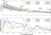 |
Fig. 1 Top: brightest spaxel spectrum for the A-star J17571324 at different dither configurations. The horizontal bars show the wavelength for two wiggles in each NRS detector. Bottom: wiggle amplitude for the brightest spaxel of the same A-star J17571324 at different dither configurations. Having more dithers reduces the wiggle amplitude, but beyond eight dithers, the amplitude of the wiggles does not decrease significantly. |
2.2 Wiggle dependence on dithering strategy
To evaluate how dithering affects the amplitude of wiggles, we processed the same A-type star observation using different subsets of dithered exposures. While the full dataset includes 16 dithers, we created reconstructed cubes using only the exposures corresponding to 1, 3, 5, 8, 12, and 16 dithers. Each subset was reduced independently using the same data reduction pipeline applied to the rest of our IFU cubes, ensuring consistent background subtraction, flat-field correction, wavelength calibration, and cube reconstruction.
For each dither configuration, we extracted the spectrum from the brightest spaxel. To isolate the wiggle spectrum, we performed an aperture extraction using a 3-pixel radius centered on the same location and subtracted this from the brightest spaxel spectrum. Since the aperture extraction effectively removes the wiggles, the residual spectrum provides a direct measurement of the wiggle in the spectrum. To quantify the amplitude of the wiggles, we divided the wiggle spectrum into wavelength slices and determined the maximum value within each slice. This allowed us to track the variation in wiggle strength in different dither configurations. As expected, increasing the number of dithers reduces the wiggle amplitude due to improved spatial sampling. However, beyond 8 dithers, the reduction in wiggle amplitude becomes less pronounced, indicating diminishing returns with additional dithers. This trend is shown in Figure 1 for the A-star J17571324 with 0.1″ spaxels and is also observed in the cubes with 0.05″ spaxels. Figure 1 also shows that the wavelength (or frequency) of wiggles remains unchanged across dither configurations. Finally, the wiggle frequencies are consistent across all NRS detectors, as expected given their instrumental origin (see Section 2.1).
3 The WICKED code
In this section, we give a detailed description of the “Wiggle Corrector Kit for NIRSpec Data” (WICKED). The workflow has three main steps that run one after the other. First, CLEAN_CENTRAL_SPAXEL fits the spectrum of the brightest spaxel to constrain the frequency correlation of the wiggles. Second, FOURIER_WIGGLE_MAP flags spaxels across the (IFU) data cube significantly affected by wiggles using the fast Fourier transform based on the frequency range of the wiggles found in the first step. Third, CLEAN_SPAXELS fits the wiggles in the flagged spaxels, removes them, and saves the cleaned spectra as a new data cube. Steps 2 and 3 in WICKED are set to run in parallel on multiple CPUs, allowing each spaxel to be handled separately and making the process faster. WICKED is available to the public and can be downloaded for free. We have made a well-documented JUPYTER NOTEBOOK example in the GITHUB repository to help users get started3.
Section 3.1 gives an in-depth description of how WICKED fits the spectra to create a model of the wiggles. Similarly, Section 3.2 describes how the wiggles are identified across the different spaxels in the (IFU) data cube using the fast Fourier transform.
3.1 Modeling the wiggles
The first step in WICKED is to create a wiggle-free model of the spectrum. This model is then subtracted from the observed spectrum to identify the wiggles. Wiggles are PSF artifacts that depend on the shape of the source; the more point-like the source, the more pronounced the wiggles in the spectrum. Therefore, in WICKED we first characterize the wiggles in the brightest spaxel of the data cube. This pixel should have the strongest wiggles, and at the same time, it has the highest signal-to-noise ratio (S/N). This spaxel serves as the reference for constraining the frequency of the wiggles in the spectrum. WICKED has a built-in method GET_CENTER to identify the brightest spaxel. In case that the wiggles are more prominent in a different spaxel, a manual entry of the spaxel location in the data cube is also possible.
WICKED fits the spectrum using two spectral templates obtained from an aperture (T1) and an annular extraction (T2), plus a power-law continuum and a second-degree polynomial. The final model is
 (1)
(1)
Here, w1,2,3 are the weights of the aperture and annular templates (T1 and T2, respectively); the power law, a1,2,3 are the power-law parameters; and b1,2,3 define the polynomial. The two integrated spectral templates (with user-defined radii) help preserve spectral features and model the line strength and spectral shape variations across the (IFU) data cube. Since wiggles are spatially correlated, integrating over multiple spaxels effectively removes them from the integrated spectral templates. The additional power-law continuum and second-degree polynomial help model any difference between the spectral templates and the observed spectrum. This is effective because many physical processes (e.g., black hole accretion, dust extinction, background) can be approximated by a power law, especially over as short wavelength range as that of a NIRSpec passband. We find that adding an additional second-degree polynomial to our models improves the quality of the fits by alleviating template mismatch at the edges of the detectors. This polynomial is also useful for fitting “bumps” in the spectra that may be caused by larger PSF artifacts, or “speckles,” which can appear around diffraction spikes for bright sources. The location of these speckles in PSF images shifts outward with increasing wavelength, i.e., they appear only at certain wavelengths for a specific spaxel, which could plausibly explain the aforementioned bumps in some spectra. The approach described here avoids using a high-degree polynomial as in Perna et al. (2023). In our tests, high-degree polynomials yielded unpredictable fits, significantly affecting the continuum shape in some parts of the spectrum. The high-degree polynomial would also “partially” fit the wiggles, jeopardizing the performance of the code in some cases.
Once WICKED obtains a good fit of the spectrum, it is subtracted from the data to obtain a wiggle spectrum. The wiggles show a sinusoidal shape with varying amplitudes and frequencies across the wavelength range. Hence, the wiggles cannot be modeled as a single sine function but as a series of different sines of the form  . We subdivide the wiggle spectrum on the basis of its peaks and valleys helping to constrain their frequencies. We found that dividing the wiggle spectrum based on a window of a random width as in Perna et al. (2023) resulted in sub-optimal wiggle removal; a window of a single width cannot properly account for the diversity of wiggles. For example, if the random width is shorter than the wavelength of the modulation, the code would model a series of smaller sinu-soidals of high frequency. In contrast, if the width was larger than the wavelength of the modulation, it would enclose wiggles of different frequencies at the same time, resulting in a worse fit.
After, the wiggle spectrum is split into different slices based on its peaks and valleys. Each slice is fitted with a sinusoidal model  . This process is repeated N times (user-defined, with a default of 15). We expect a relation between the wavelength and frequency of the wiggle from the way the diagonal spectral trace crosses the detector grid (Law et al. 2023). This relation was used in Perna et al. (2023) to improve the fitting of the sinusoidal model, using it as the prior to the frequency in each slice. We found the same trend, and have adopted their method in the WICKED code. For each slice, we save the best-fit frequency ƒλ and the central wavelength. A five-degree polynomial is then fit to the ƒλ and central wavelength in each iteration to constrain the wiggle frequency ƒλ − λ relation. This is then used as a prior for finding the best ƒλ in the subsequent iterations. The polynomial fit is updated with the new frequencies in each iteration if the new frequencies pass a chi-square threshold set by the first iteration. This ensures that only good fits are saved, preventing poor fits from negatively impacting the polynomial fit of the ƒλ − λ relation. Finally, in the last iteration, the best-fit wiggle model is subtracted from the brightest spaxel, correcting for the undesired wiggles.
Figure 2 shows the output of the CLEAN_CENTRAL_SPAXEL step in WICKED that fits the data and constrains the ƒλ − λ relation of the wiggles for the brightest spaxel of the data, in this case of the A-star J1757132. The top panel of Figure 2 shows in red the spectrum of the brightest spaxel for J1757132, with the two integrated spectrum templates in gray and yellow. The best-fit model built from the spectral templates, the power law and the polynomial is shown in blue. The middle panel of Figure 2 shows the wiggle spectrum (gray) and the best wiggle model (red) obtained by WICKED. Highlighted as green crosses are the identified peaks and valleys used to split the wiggle spectrum. The bottom panel shows the corrected spectrum (red) and the residuals (gray) between the best-fit model and the corrected spectrum. WICKED automatically finds the most prominent emission/absorption lines (based on their signal-to-noise ratio) in the spectrum which are excluded during wiggle fitting. These are shown as red vertical lines, and the yellow region is the excluded gap between the two NIRSpec detectors.
The process described here is repeated for each spaxel of the data cube (inside a search radius, see more details in Section 3.2), with an adjusted second-degree polynomial and power-law coefficient for each. The ƒλ − λ relation found for the brightest spaxel is used as a prior to fit for ƒλ in each spaxel.
3.2 Flagging spaxels with wiggles
The identification of spaxels in the data cube affected by wiggles is performed in the FINDWIGGLES.FOURIER_WIGGLE_MAP step in WICKED. In this step WICKED calculates the fast Fourier transform of the wiggle spectrum using the SCIPY package SCIPY.FFT. The resulting Fourier spectrum (ℱS pec) is divided into two sections; one part dominated by wiggles and the rest of the spectrum. The part of the Fourier spectrum dominated by wiggles is defined based on the frequencies found during the CLEAN_CENTRAL_SPAXEL step for the brightest spaxel. The frequencies of the wiggles depend on the compactness of the source, typically ranging between 5–60 [µm−1]. The mean amplitude and standard deviation for these two parts of the Fourier spectrum are then compared to identify spaxels with wiggles. The mean amplitude plus the standard deviation (a 1-σ value) for the part of the spectrum not dominated by wiggles give us information about the amplitude of the stellar features and the noise in the spectrum. We use this as a benchmark and compare it to the mean amplitude of the Fourier spectrum at frequencies dominated by wiggles. For spaxels affected by wiggles, the ratio of these two Fourier amplitude values (hereafter “Fourier ratio”) is larger than one. The Fourier ratios are
 (2)
(2)
Here, Fratio is the Fourier ratio, and ƒwiɡɡle represent the maximum frequency of the wiggles. The default Fourier ratio in WICKED is Fratio = 3, and we recommend always using a value of Fratio ≥ 1.5 (see Section 4.1). Figure 3 shows an example of how the wiggle detection is performed in WICKED for the brightest spaxel of the F170LP cube of the A-star J1757132. Figure 3 shows the output of FINDWIGGLES.PLOT_WIGGLE_FFT built-in method in WICKED developed to examine the Fourier spectrum and the Fourier ratio of a particular spaxel. The output of PLOT_WIGGLE_FFT consists of 3 panels, showing the spectrum of the spaxel, the wiggle spectrum and its Fourier spectrum. We show two of the three panels in Figure 3. Figure 3 left, shows the resulting wiggle spectrum (red, described in Section 3.1) and the masked regions (pink). The right panel shows the Fourier spectrum for the NRS1 (red) and NRS2 (dark red) part of the spectrum. The red shaded region shows the range of frequencies dominated by wiggles (identified during Step 1, see Section 3.1). The Fourier ratio for the brightest spaxel of the A-star J1757132, is ~5.5. This ratio is calculated as the mean amplitude of the NRS Fourier spectrum affected by wiggles (horizontal fuchsia line) divided by the 1-sigma value (mean amplitude + standard deviation) of the rest of the Fourier spectrum (blue horizontal dashed line).
WICKED calculates the Fourier spectrum separately for both NRS detectors and uses the part of the spectrum where the Fourier ratio is largest to flag the spaxel. We adopted this approach because the amplitude of the wiggles depends on the signal-to-noise of the source in the NRS detector. Using the spectrum from the NRS detector less affected by wiggles would lower the overall mean amplitude at wiggle-dominated frequencies, thus reducing the ability of WICKED to accurately flag the spaxel.
During the FINDWIGGLES.FOURIER_WIGGLE_MAP Step, each Fourier spectrum is calculated in parallel inside a search radius (default 10 pixels) which speeds up the process. Since the Fourier ratio for a given spaxel is only known after this step is complete, we developed a method called FINDWIGGLES.DEFINE_AFFECTED_PIXELS to set the Fourier ratio threshold. This function allows users to define a Fourier ratio threshold and view a map of flagged spaxels across the data cube, without the need to re-run FINDWIGGLES.FOURIER_WIGGLE_MAP each time the threshold is adjusted. Once an optimal threshold is defined using FINDWIGGLES.DEFINE_AFFECTED_PIXELS, the FITWIGGLES.CLEAN_SPAXELS step is used to fit and remove the wiggles from each spaxel. The corrected spectra are then saved in a new data cube.
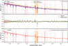 |
Fig. 2 Correction of the brightest spaxel in the F170LP cube of the A-star J1757132 using the CLEAN_CENTRAL_SPAXEL step in WICKED. The top panel shows the original spectrum (red) with prominent wiggles. The aperture (3-pixel radius) and annular integrated (3- to 5-pixel annular radius) spectra are displayed in gray and yellow, respectively, with the best-fit model shown in blue. Subtracting this smooth model from the single spaxel data produces the wiggle spectrum (middle panel, gray). WICKED identifies peaks and valleys in the wiggle spectrum (green crosses) and fits a wiggle model (red), which is subtracted to produce the final wiggle-free spectrum (bottom panel, red), pink vertical lines mark masked regions, while the yellow area highlights the gap between the NRS1 and NRS2 detectors. |
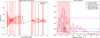 |
Fig. 3 Example of a wiggle spectrum and its fast Fourier transform for the spectrum of J1757132. The fast Fourier transform is used in WICKED to flag spaxels in the data cube affected by wiggles. The built-in method PLOT_WIGGLE_FFT in WICKED allows for manual examination of the spectrum and its Fourier transform for a specific spaxel in the data cube. The left panel shows the wiggle spectrum created by subtracting the spectrum from the best-fit model. The right panel shows the Fourier transform of the wiggle spectrum. The solid fuchsia line represents the mean amplitude in the wiggle-dominated part of the spectrum (shaded red region). WICKED flags the spaxels by comparing the mean amplitude to the standard deviation (blue dashed line). If the data from the two NRS detectors are available, as in this case, WICKED determines which part of the spectrum shows the most prominent wiggles and bases the flagging on that part of the spectrum. |
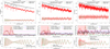 |
Fig. 4 Comparison of the spectrum of the A-star J1757132 (top, black) and the degraded spectrum (top, red) with the added wiggle model (green) at S/N ratios of 50, 15, and 8. Middle: Fourier spectra of (i) the degraded spectrum (solid, red), (ii) the wiggle model (green), (iii) the degraded spectrum without wiggles (black), and iv) the data corrected with WICKED (dashed, red). The horizontal lines mark the mean amplitude of the Fourier spectrum at frequencies dominated by wiggles and at larger frequencies. The Fourier ratio can effectively distinguish wiggles from noise down to a S/N ratio of ~8. Bottom: comparison of the input wiggle model (green) versus the recovered wiggle spectrum for the data cleaned with WICKED. |
4 Quantifying WICKED’s performance
In this section we show the results of different tests designed to evaluate WICKED’S ability to identify wiggles and recover the spectrum at different S/N ratios. We also compare WICKED’S performance to the method by Perna et al. (2023). The method by Perna et al. (2023) requires fine tuning of parameters, which depend on the source and needs to be explored by the user. In this work, we use the default parameters as presented in the available GitHub repository. This may underestimate the performance of the method by Perna et al. (2023) but first, it helps with the reproducibility of our tests and second, we are interested in the performance of WICKED and we only use the method by Perna et al. (2023) as a base of comparison. The tests were performed using the spectrum of the A-star J1757132 and the M-star J15395077. The PSF aperture-extracted (3 pixel radius) spectra of these stars serve as known, wiggle-free references for our test. The A-star J1757132 was chosen for its high S/N (~500) and prominent hydrogen lines, which we use to test the impact of the code on the line strength measurements. We created a wiggle model from the difference of the integrated spectrum of J1757132 and its brightest spaxel. In the upper left panel of Figure 4 the integrated spectrum of the A-star J1757132 is shown in black, and the wiggle model in green.
To simulate various scenarios, the wiggle model was manually added to the integrated spectrum of J1757132 along with Gaussian random noise to achieve different target S/N ratios. Using this method, we created data cubes for the integrated spectrum of J1757132 at S/N ratios of ~500, 400, 300, 200, 150, 100, 50, 15, 10, and 8. For each data cube, we saved the noisy spectrum with wiggles, and the noisy spectrum without wiggles at different spaxel in the outer parts of the data cube. This allowed us to process the data cube using WICKED and the code by Perna et al. (2023) without modifying the codes. To account for Gaussian random noise variability, we created ten individual data cubes for each S/N ratio by adding different noise realizations, resulting in a total of 100 data cubes. Generating multiple cubes for each S/N ratio also allowed us to quantify systematic uncertainties during the wiggle removal by both WICKED and the method by Perna et al. (2023).
In Section 4.1, we present the ability of our Fourier-ratio-based method to identify wiggles at different S/N ratios. In Section 4.2 we further test the stability of the shape of absorption lines and the continuum in the spectrum (S 4.2). For simplicity, in the test we used only the spectra in the NRS1 detector, which exhibits the largest wiggle amplitudes for J1757132. The results of our test should not be affected by this choice, as the wiggle frequencies are nearly identical across both NRS detectors, differing only in amplitude. Finally, in Section 4.3 we evaluate how well WICKED preserves the overall kinematics by looking at the integrated spectrum of the M-star J15395077.
4.1 Fourier ratio sensitivity to detect wiggles
To get a sense of up to which S/N the Fourier ratio method used in WICKED can reliably detect wiggles in a spectrum, we examined the Fourier spectrum of J1757132 at different S/N values and compared the Fourier ratio for spectra with and without the wiggle model. In Figure 4, we present the Fourier spectra for our three lowest S/N cubes (50, 15, and 8) to illustrate how this method separates wiggles from noise. The original aperture spectrum of J1757132 (S/N ~500) is shown in the top panel in black, and the degraded spectra in red. In the top panel of Figure 4 we also show the original wiggle model (green) added to the data, and the version with added noise (red). The wiggle spectrum (top, red) is obtained by subtracting the best-fit model from the degraded spectrum (with added noise) and represents what WICKED will try to fit, as described in Section 3.1. However, as the S/N decreases, the wiggles begin to blend with the noise, making them harder to detect by visual inspection alone. For spectra with S/N ≤ 15, distinguishing wiggles from noise becomes unreliable without a mathematical approach similar to the Fourier ratio.
The middle panel of Figure 4 shows the Fourier spectrum for each spectrum at a given S/N (solid, red), for the degraded spectrum without adding the wiggle model (black), and for the spectrum corrected with WICKED (dashed, red). The Fourier spectrum of the wiggle model (green) is also shown in the middle panel of Figure 4. The Fourier spectrum of the wiggle model has two large peaks at frequencies ƒλ ≈ 20, 40 [µm−1], but it has hardly any feature at frequencies ƒλ > 60 [µm−1]. In contrast, the Fourier spectrum for the degraded spectrum without the added wiggles (black) regardless of the S/N, shows similar levels of features at all frequencies and lacks the two peaks at ƒλ ≈ 20, 40 [µm−1] seen in the wiggle model Fourier spectrum. The Fourier spectrum for the degraded spectrum with added wiggles (red) shows the spectral features at ƒλ > 60 [µm−1] almost identical to the spectrum without the added wiggles, and the two prominent peaks from the wiggle model at ƒλ ≈ 20, 40 [µm−1]. Finally, the Fourier spectrum of the data cleaned with WICKED closely matches the reference Fourier spectrum of the data without wiggles, showing that the two prominent peaks have been largely removed, and at a S/N of 8 we still remove ~50% of the wiggle signal.
The horizontal lines in Figure 4 are similar to the ones in Figure 3, but since here we compare three Fourier spectra at once we have changed the colors. The fuchsia line in Figure 4 marks the mean amplitude for the degraded spectrum with added wiggles, and the black line for the degraded spectrum without wiggles (in the wiggle regime). These two values are never the same at any S/N, while the blue line is almost identical to the mean amplitude (solid blue line) at frequencies outside the wiggle regime of the spectrum with the added wiggles. This shows that the wiggles and the spectral features are in completely separate parts of the Fourier spectrum. When we look at the Fourier ratio, used to flag spaxels in WICKED, we see a clear tendency; at higher S/N the Fourier ratios are higher (~14 at S/N of 50) and ~1.5 at S/N 8. The Fourier ratio changes because the 1-σ benchmark (blue dashed line) for the part of spectrum outside frequencies dominated by wiggles increases at lower S/N, while the mean amplitude for the wiggle regime (fuchsia line) remains almost the same.
The bottom panel of Figure 4 shows the recovered wiggle spectrum with WICKED and compares it to the true wiggle model. At a S/N of 50 both are mostly identical, having a mean difference of only 1.7 ± 1.9% and a maximum difference of ~7% for the wiggles at ~1.9 µm. At a S/N of 15 we can see larger difference not only in the lower amplitude wiggles around ~1.9 µm but also in the more prominent wiggles around 2.3 µm. However, the differences are still 3.4 ± 2.8% on average with a maximum value of ~12% around ~2.15 µm. Interestingly, this is close to an absorption line (LINE 3 in Figure 5) that is masked during the cleaning with WICKED, which could explain the larger difference. Finally, at a S/N of 8 we observe the largest difference in the recovered wiggle spectrum, with an average difference between the WICKED-clean and degraded aperture spectrum of 5.5 ± 4.5%, only ~500 [MJy/sr], which is about 5× smaller than the average noise (~2700 [MJy/sr]).
In summary, the Fourier transform is quite reliable at distinguishing wiggles in the spectrum versus Gaussian random noise. The Fourier ratios are more than ≥3 σ larger than the amplitude of the spectral features for spectra with a S/N ≥15 in the presence of large wiggles as simulated by our wiggle model. The Fourier ratio decreases quickly, becoming only ~1.5 σ at a S/N of 8. The recovered wiggle spectrum after cleaning the spectrum with added noise in WICKED, shows insignificant differences at high S/N, with more than 80% of the wiggles signal removed at S/N of 50. At lower S/N, the mean differences increase, and there are also more often larger differences between the recovered and the original wiggle model. However, as mentioned above this difference are still in average smaller than the noise and with most of the wiggles signal removed from the data (~50%). Based on this, we recommend using WICKED with a Fourier ratio Fration ≥ 1.5. We cannot directly compare WICKED’s ability to flag spaxels with wiggles to the code developed by Perna et al. (2023), as their method uses a different technique based on a S/N threshold (defined by the user) with respect to the brightest spaxel, which is not comparable to the method presented here.
4.2 Preservation of continuum and lines shape
To evaluate how well WICKED preserves the shape of the absorption lines in the spectrum, we study the equivalent width (EW) of three absorption lines in the spectrum of J1757132 at various S/N ratios. There are no gas emission lines in the spectrum of J1757132, but there should be no practical difference on how WICKED deals with emission or absorption lines. We also evaluate how WICKED preserves the overall spectral shape by comparing the mean difference of the spectrum at different S/N ratios with respect to the aperture spectrum of J1757132. We also do this for the spectra without the added wiggles, to simulate the impact of wrongly flagged spaxels cleaned in WICKED, and its impact in its spectral shape. We compare all our results with the cubes cleaned using the method by Perna et al. (2023).
The EW for each line was determined by multiplying the FWHM by the flux at the minimum of the absorption line. The errors in the EW were calculated using the 50 Monte Carlo simulations based on the error array. The results of the test for the EW are shown in Figure 5. The top panel of Figure 5 shows the aperture spectrum of J1757132 and the three absorption lines used for the EW comparison marked in blue. We compare the EW for three different lines since they are affected differently by wiggles because the amplitude and frequency of the wiggles change with wavelength. The bottom left panel shows the profile for one of these lines, “LINE 1”. The solid black line is the line profile for the aperture spectrum (S/N of 500), the dashed gray line for the uncorrected spectrum (the output of the JWST pipeline), the red line for the spectrum cleaned with WICKED, and finally in yellow for the spectrum cleaned with the method by Perna et al. (2023). The right panel shows the percentile difference for each line for the different data cubes at different S/N compared to the “true” EW. The true EW is defined as the value obtained from the degraded spectrum at that S/N without added wiggles.
The differences in EW are quite similar across all the different S/N ratios, and they are mostly dominated by the amplitude of the wiggle model. For the uncorrected spectrum (gray symbols), LINE 1 that is in the region of the spectrum with large amplitude wiggles, has a difference of ~20%, while the rest of the lines show a difference of ~10%. Based on this test we expect EW biasses larger than typical error (~4%) down to spectra with a S/N of 50. For the spectra cleaned using WICKED (red symbols), we see similar differences in EW regardless of the S/N and the absorption line with a mean difference of only 3.5%. This difference is ~4× smaller than the average difference for the uncorrected spectra (14%), and more than 2× smaller than the average difference for the spectra cleaned with the method of Perna et al. (2023) (7.2%). This shows the ability of WICKED to remove wiggles of different amplitudes and frequencies across the whole wavelength range with the same quality. This is not the case for the spectra cleaned with the method by Perna et al. (2023), where LINE 1 has almost 2× larger difference in EW as the other two lines. LINE 1 is located near the low-wavelength edge of the spectrum, while the other two lines are in the middle.
We observe this discrepancy in the ability to remove wiggles at the edges of the spectrum in the method of Perna et al. (2023) across all our tests in this work (see, for example, Figure 7).
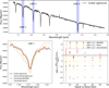 |
Fig. 5 Comparison of recovered EWs for two absorption lines present in the spectrum of the A-star (solid black line) J1757132. The bottom-left panel shows the profile of the LINE 1 for the original spectrum (solid black), the spectrum with wiggles (dashed), and the spectra corrected using WICKED (red) and with the code by Perna et al. (2023) (yellow). The line profile and EW are better recovered with WICKED than with the code by Perna et al. (2023), with the corrected spectrum having a less than 5% difference with the “true” value derived from the spectrum with no wiggles. For the uncorrected spectrum (gray), we observed EW differences exceeding the typical error (4%) in spectra with S/N as low as 50. |
4.2.1 Mean flux difference
To quantify how the overall shape of the continuum is preserved during the cleaning with WICKED, we calculate the mean flux difference of the spectrum with added wiggles at various S/N versus the aperture spectrum. This helps quantify the overall disagreement between the “true” (the aperture spectrum of J1757132) spectrum and a corrected spectrum processed with either WICKED or the method by Perna et al. (2023). The uncertainties are calculated from the standard deviation of the mean flux difference for the 10 corrected cubes at this particular S/N. As mentioned above we created 10 cubes at each S/N to help constrain the systematic errors introduced by cleaning the spectrum. Additionally, misclassifìcation of spaxels across the data cube is a possibility, and thus we also tested the impact in the spectrum in the case a spaxel with a “clean” spectrum (i.e without wiggles) was wrongly flagged and cleaned with WICKED and the code by Perna et al. (2023).
The results are shown in Figure 6. The mean flux difference between the spectrum without added wiggles at that particular S/N and the aperture spectrum are shown as black rectangles in Figure 6, with the height representing the 1 σ uncertainty. These black rectangles serve as a benchmark for comparing how well the overall shape of the spectrum is preserved. In Figure 6 we can see that the mean flux difference for the uncorrected spectrum (shown in gray stars) is dominated by the amplitude of the wiggles at high S/N, while at S/N ≤ 50 by the Gaussian random noise of the spectrum. At low S/N ratios some of the differences introduced in the spectrum by the wiggles get lost in the noise of the spectrum.
For the spectrum with wiggles (solid symbols) in Figure 6, the spectra cleaned with WICKED (red squares) show the smallest mean flux difference across all S/N when compared to the uncorrected spectra and the ones cleaned using the method from Perna et al. (2023) (yellow squares). On average the spectrum cleaned with WICKED has a ~4× smaller mean flux difference compared to the uncorrected spectrum, and ~1.4× than the one cleaned using the method by Perna et al. (2023) down to a S/N ratio of 50. This means that if a spaxel in the data cube is correctly flagged (to have wiggles) the resulting spectrum will always be better than the output from the JWST pipeline, or by cleaning it with the method by Perna et al. (2023).
The spectra without wiggles that were still cleaned using WICKED and the method by Perna et al. (2023) are shown in open squares in Figure 6. At high S/N both codes “impair” the spectrum by trying to correct for wiggles when they are not present, although the differences are very small. At S/N of 500 and 400 the spectrum cleaned using WICKED the differenc is only ≤50 [MJy/str], which is of the same order as the average error of the spectrum (~54 [MJy/sr]). This difference becomes ~25 [MJy/str] at a S/N of 200, which is 4× smaller than the average error. At smaller S/N the difference continues to decrease until it becomes comparable to the uncertainties of the benchmark rectangles. The mean flux differences are close to half smaller for the spectrum cleaned using the method by Perna et al. (2023) compared to WICKED at S/N ⪆ 200. However, the difference between the two methods becomes comparable at about S/N of 150. This difference between WICKED and the method by Perna et al. (2023), and the fact that the mean flux difference for WICKED seems to be slightly lower than the benchmark rectangles at very low S/N, could indicate that WICKED is more prone to over-fitting. However, as mentioned above, we emphasize that the differences are very small. Finally, as shown in Section 4 WICKED is quite reliable at flagging spaxels affected by wiggles down to a S/N ~ 8. Thus, it is unprovable for WICKED to incorrectly flag a spaxel at high S/N ratios, and consequently affecting the quality of the spectrum.
In our test we have observe that a high S/N spectrum can be misclassified and significantly affected if there is a large mismatch between the best fit-model and the data. We recommend the users to never run WICKED blindly, and always inspect for spaxels that could be incorrectly flagged. These spaxels can be excluded from the fitting using the keyword DEFINE_AFFECTED_PIXELS.EXCLUDE_PIXELS (Please see the example JUPYTER NOOTEBOOK in the GITHUB repository for details).
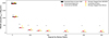 |
Fig. 6 Comparison of the mean difference flux with respect to the aperture spectrum of the A-star J175713. The black rectangles represent the minimum expected the flux difference at a given S/N ratio. The spectra corrected using WICKED (solid red) shows the smallest mean flux difference compared to the uncorrected spectrum (gray) and the spectrum clean using the method by Perna et al. (2023) (solid yellow) at all S/N. |
4.2.2 Changes in the spectra across the field of view
Spatial variations in the spectra across the data cube, such as those caused by differential dust obscuration or contributions from different sources, can lead to mismatches between the two stellar templates and the spectrum at a given spaxel. Such is the case, for example, in NGC 5128, where the bright central AGN dominates the spectra in the inner regions, while at larger radii the stellar component becomes more prominent. This transition leads to a significant change in the continuum slope across the field of view. In such cases, the best-fit model may rely more heavily on the power law and second-degree polynomial to account for these differences.
We simulated this scenario by creating a “dust-obscured” spectrum of the aperture spectrum of J1757132. We used the infrared-optical extinction law from Cardelli et al. (1989) to add dust component with a value of AV = 20. The obscured spectrum was saved in the spaxel Xspaxel = 16, Yspaxel = 16 and then cleaned using WICKED and the method by Perna et al. (2023), similarly as done for the previous cubes (S 4).
The resulting obscured spectrum is shown in black in the left panel of Figure 7. Figure 7 also shows the clean spectrum using WICKED (red) and the code by Perna et al. (2023) (yellow). We also show the clean spectrum without the added dust obscuration to have a side-by-side comparison of their differences. The middle panel shows the relative flux difference between the clean and the integrated spectrum. Colors are the same for all the panels. The bottom shows the recovered wiggle spectrum by WICKED and the code by Perna et al. (2023) and the original wiggle model (green).
As expected from the results of Section 4.2.1, the spectrum cleaned with WICKED has lower relative differences with respect to the one done with the method by Perna et al. (2023) for the spectrum without dust obscuration. The spectrum cleaned with WICKED shows relative flux differences around 0 with some small section in the spectrum with differences of ~4%. However, the spectrum cleaned with the method by Perna et al. (2023) have a large portion in the spectrum between 1.7–1.8 µm with differences of ~8%. The situation is worsened for the obscured spectrum, where the data cleaned with the method by Perna et al. (2023) shows about 3× larger differences in that section, with relative differences of ~25%. For the spectrum clean with WICKED, however, the differences are relatively the same as for the un-obscured data with no large portion of the spectrum with large differences, only having a maximum difference of ~6% around an absorption line in ~1.8 µm. The spectrum corrected with the code by Perna et al. (2023) also shows a small “dip” in the continuum for the un-obscured spectrum in the 2.7–2.9 µm region. These results support the use of a power law plus a simple polynomial (second-degree) to model mismatches between the spectrum and the integrated templates, over the high degree polynomial used in Perna et al. (2023).
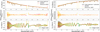 |
Fig. 7 Comparison of WICKED and the code by Perna et al. (2023) at correcting for wiggles. The left panel shows the performance of both codes at recovering the wiggles model (shown in black in the bottom panel) added to the spectrum of the A-star J1757132 (solid black line). In the right panel we compare the performance of both codes at recovering the wiggles when the shape of the continuum is different from the integrated spectrum. We modified the spectrum by adding dust extinction with a value of AV = 20, using the Infrared-Optical relation by Cardelli et al. (1989). As shown WICKED is better at recovering the wiggle then the code by Perna et al. (2023), specially when the integrated spectrum is not a perfect model for the spectrum. |
4.3 Enabling line-of-sight velocity measurements with WICKED
The presence of wiggles can significantly distort line shapes (see bottom-left panel of Fig. 5), impacting the ability to obtain reliable kinematic fits for NIRSpec at a single-spaxel level. In this section we show how WICKED can effectively subtract these artifacts to obtain reliable kinematics that otherwise could not be possible. For this we used the F170LP NIRSpec data cube of the M-star J15395077 rather than the previously used A-star J1757132. A-stars lack the Carbon Monoxide (CO) bandhead at 2.30 µm series commonly used for stellar kinematics, while they are the dominant stellar feature in M-stars. The spectrum of 2MASS J15395077 was reduced in the same way as the data of J1757132 and corrected for wiggles using both WICKED and the code by Perna et al. (2023). We obtained the line-of-sight velocities (LOSVs) and velocity dispersion (σ) for the brightest spaxel of the F170LP cube J15395077, for three different cubes; first an uncorrected cube, second for the cleaned cube using WICKED, and the last cube cleaned using the method by Perna et al. (2023). The LOSV and σ were extracted using the PYTHON implementation of the penalized spaxel fitting routine, PPXF (Cappellari 2017) with a set of synthetic high-resolution stellar templates from the Phoenix library (Husser et al. 2013). A fifth-degree additive polynomial was used to model the continuum differences between the spectrum and the templates. Uncertainties for the LOSV and σ were estimated using a boot-strap method. We compare the resulting LOSV and σ against an aperture-extracted spectrum with a 0.15″ (3-pixel radius), close to the PSF value. This effectively reduces the sinusoidal modulations since they are spatially correlated and thus tend to cancel out. Since the quality of the PPXF fit is a function of the S/N of the data, we degraded the aperture spectrum of J15395077 from its native S/N ≈ 150 to a S/N of 41 to match the S/N of the brightest spaxel of J15395077.
The left panels in Figure 8 show the best-fit model with PPXF (blue) for the four different spectra, and the right the residuals. The degraded aperture spectrum (black) has a best-fit line-of-sight velocity of VLOS V = −119.4 ± 2.9 km s−1. The un-degraded aperture spectrum (with a S/N of 150) has an LOSV of VLOS V = −114.9 ± 2.7 km s−1, perfectly matching the Gaia DR3 catalog value for this object (Riello et al. 2021). It is clear in Figure 8 that for the uncorrected data cube (gray), PPXF cannot find a good fit due to the pronounced wiggles in the continuum, resulting in a poorly fit LOSV of VLOS V = 25.2 ± 53.6 km s−1, clearly inconsistent with the star’s LOSV. For data cubes corrected for wiggles, both WICKED (red) and the code by Perna et al. (2023) (yellow) yield reliable PPXF fits, with LOSV values of VLOS V = −121.0 ± 4.4 km s−1 for WICKED and VLOS V = −122.5 ± 6.4 km s−1 for the code by Perna et al. (2023), both consistent with the aperture-extracted spectrum’s LOSV within error. We note that the LOSV uncertainty for the WICKED-corrected spectrum is about 50% smaller than that obtained with the Perna et al. (2023) method, likely due to WICKED’S superior wiggle removal. The velocity dispersion for this star is below NIRSpec’s instrumental resolution, so it cannot be properly estimated and we expect PPXF to give a velocity dispersion ~0 km/s. However, the degraded aperture-spectrum and the data cubes corrected with WICKED and the Perna et al. (2023) method all agree on a velocity dispersion of 0.6 ± 0.0 km s−1. In contrast, the uncorrected data cube shows an unrealistic value of 449.4 ± 101.2 km s−1, underscoring the impact of wiggles on determining reliable velocity dispersions. Without correction, PPXF misinterprets broad wiggle features as actual spectral features, leading to inaccurate fits.
The right panels of Figure 8 show the residual between the data and their best PPXF fit. The method of Perna et al. (2023) is less effective. The residuals for the spectrum corrected using WICKED are mostly flat and dominated by remaining outliers from the JWST pipeline, while for the spectrum corrected using Perna et al. (2023) there are plenty of residual wiggles in the spectrum. We also note that the spectrum corrected using the method by Perna et al. (2023) leaves a slightly “concave” residual shape when compared to the aperture-extraction spectrum. The “concave” residual in the continuum might be improved by manually changing the polynomial degree used to fit the continuum in Perna et al. (2023). However, this “concave” effect is not visible in the bottom panel of Fig. 8 because the added polynomial using during the PPXF fit. This change in the continuum was not visible for the spectrum corrected using WICKED.
Finally, without wiggle correction, single-pixel kinematics measurements for the spectrum similarly affected by wiggles to this M-star would be impossible, and in other cases would make it significantly challenging and bias the results. However, WICKED can effectively remove wiggles, allowing kinematic analysis at the single-pixel level, with WICKED providing better results than the method used by Perna et al. (2023).
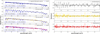 |
Fig. 8 Left: PPXF fits (blue) for the integrated spectrum (black) of the M-giant star J15395077, uncorrected brightest spaxel spectrum (gray), spectrum corrected with the code by Perna et al. (2023) (yellow), and spectrum corrected using WICKED (red). The FWHM aperture spectrum was degraded to match the S/N of the brightest spaxel of the cube. The best-fit LOSV and velocity dispersion for each spectrum are shown in the blue text boxes. We see that for an uncorrected spectrum it is not possible to obtain a reliable fit due to the wiggles, having a difference ~145 km s−1 with the LOSV of the integrated spectrum, three times larger than the estimated uncertainty. While, for both the spectrum corrected using WICKED and the code by Perna et al. (2023) a good fit can be achieved, with both being consistent within uncertainties with the LOSV of the integrated spectrum (wiggles-free). We note that using WICKED we obtain a best-fit value closer to the “true” value of 119.9 ± 2.7 for the integrated spectrum, and an uncertainty ~45% smaller than for the spectrum corrected with the code by Perna et al. (2023), which is probably due to the superior performance of WICKED at removing the wiggles. Right: residuals between each spectrum and the best fit. One can see that the residuals for the spectrum corrected using WICKED (red) are flat and mostly dominated by outliers left during the data reduction with the JWST pipeline, while for the spectrum corrected using the code by Perna et al. (2023) there are plenty of residual wiggles. |
5 Stellar and gas kinematics: Case study of NGC 5128
In the following section, we present the stellar and gas kinematics for the NIRSpec observations of NGC 5128, hereafter Centaurus A. We showcase the kinematics of Centaurus A as a practical example of the science that can be achieved after correcting for “wiggles” with WICKED. Centaurus A serves as a perfect example for this, since its nuclear kinematics has been well studied previously (e.g., Silge et al. 2005; Marconi et al. 2006; Neumayer et al. 2007; Cappellari et al. 2009), making it a perfect benchmark for comparing our results.
We focus our kinematic analysis only in the F170LP observations, since it contains the 2.30 µm (2−0) 12CO bandhead and two of the other prominent 12CO series, commonly used for the dynamical modeling of black hole masses, as well as hydrogen molecular and hydrogen recombination lines Paα, Brγ and Pfδ. We removed wiggles from the F170LP observation using WICKED, with a Fourier ratio of 3.5σ leading to 120 spaxels flagged.
The spectrum of Centaurus A shows prominent hydrogen recombination lines in the wavelength range of the F170LP, such as Paα, Brγ and Brβ. Hydrogen recombination lines can be excited by the radiation field of the central AGN in the narrow-line region, but they can also come from radiation from ongoing star formation. In this wavelength range there are also a few important molecular hydrogen lines at 1.95 µm 1−0 S(3), 2.03 µm 1−0 S(2), 2.12 µm 1−0 S(1). There are also several different ion lines such as [Si Vi], [OIII], [MgII], etc. In this work we do not intend to make an exhaustive study of the kinematics of the different emission lines, but extract the overall kinematic properties of the gas and stars in Centaurus A and compared them with previous results of Neumayer et al. (2007) for the gas kinematics and Cappellari et al. (2009) for the stellar kinematics. Please refer to those works for a more in-depth review of the kinematics of Centaurus A, as well as Neumayer (2010).
In order to increase the S/N, we spatially bin the WICKED-cleaned data cube using the Voronoi PYTHON package VORBIN (Cappellari & Copin 2003) to achieve a S/N of 100, resulting in 515 bins, with most of the bins inside the 0.5″ consisting of a single spaxel. We fitted the spectrum of the individual bins using (PPXF) (Cappellari 2017) in the spectra range of 1.7–3.16 µm, with the synthetic high-resolution stellar templates from the Phoenix library (Husser et al. 2013), in the same manner as described in Section 4.3. We simultaneously fit the hydrogen recombination lines, molecular lines, and stellar absorption in PPXF, assigning separate kinematic components to each. For the gas, we fit the first two velocity moments, while for the stars, we also include the third and fourth Gauss-Hermite moments (h3 and h4). The typical uncertainties in LOSV and velocity dispersion for individual bins are 6 km s−1 and 5 km s−1, respectively. As mentioned in Cappellari et al. (2009), the nuclear non-thermal component in Centaurus A dominates the total flux at radii ≲0.2″ and dilutes the stellar features in the spectrum. Therefore, it is advisable to use a fixed set of stellar templates to correctly model the spectrum and obtain reliable kinematics in the nuclear region (Cappellari et al. 2009). We define a set of stellar templates selected from the fit of an annular spectrum of Centaurus A, to exclude the nuclear non-thermal continuum. Based on the surface brightness profile for Centaurus A of Cappellari et al. (2009, Fig. 6), the non-thermal and stellar continuum are equal at a radius of ~1.0″, so our annular spectrum is extracted between a radii of 1.0–1.3″. The pPXF fit for the annular spectrum resulted in 9 Phoenix templates with temperature ranging from 2800–4600 K and metallicity −4.0 to −0.5 [M/H].
An example spectrum for an off-center spaxel at a radius of 0.15″ from the center for the uncorrected cube (top, black) and the cube corrected with WICKED (bottom, red) are shown in Figure 9. Their best PPXF fit is shown in blue for both spectra and their best-fit LOSV and σ in the blue box. In this example, we can see the effect that the wiggles have in determining the LOSV and σ and also in determining emission lines with PPXF. The wiggles in the uncorrected spectrum bias the best-fit LOSV to a value much larger than the 531 ± ΔV = 20 km s−1 reported in Cappellari et al. (2009) inside the 1.5″. The LOSV value for the spectrum corrected with WICKED is in great agreement with this value. Similarly for the velocity dispersion σ, since the model tries to fit the wide features of the wiggles as if they were stellar features, the fitted σ is biased high for the uncorrected cube, to values unrealistically higher than the maximum value of ~165 km s−1 from Cappellari et al. (2009). The wiggles also affect the ability to detect emission lines in the spectrum. For the uncorrected spectrum PPXF confuses a wiggle at 3.13 µm as the [OIII] line, while in the corrected spectrum with WICKED it is not present. In general, for spaxels affected by wiggles (radii ≤0.4″), we observe an average difference of ~ 181 km s−1 and ~ 104 km s−1 for the LOSV and velocity dispersion between the uncorrected cube and the WICKED-cleaned cube, respectively (right-panel in Figure 9). This difference is about 36× and 17× the average uncertainty for the LOSV and velocity dispersion, respectively.
The extracted gas kinematics for the F170LP cube corrected with WICKED for the hydrogen recombination lines and hydrogen molecular lines and the difference between the two are shown in Figure 10. The velocity map for the molecular hydrogen (middle panel in Fig. 10) is smooth and symmetric with a clear regular rotational pattern and a maximum rotation velocity of ΔV ≈ 123 km s−1. The velocity map also shows the same twist in the major axis of rotation reported in Neumayer et al. (2007). Overall the kinematics of the molecular hydrogen is in good agreement with the results from Neumayer et al. (2007). The kinematics for the hydrogen recombination lines on the other hand also shows a clear rotation, but it seems to be somehow influenced by the Centaurus A’s radio-jet. The difference in the velocity pattern between the two is clear when we plot their difference (right panel, Fig. 10. Their difference shows a dip in velocity in the region (0.5″, −0.5″) which is close to the knot in the radio jet shown in Neumayer et al. (2007). The velocity map for Brγ from Neumayer et al. (2007) aligns well with our hydrogen recombination line results, which include Brγ.
Figure 11 shows the stellar LOSV, velocity dispersion and the first two Gaussian–Hermite moments. The strong non-thermal continuum in the nuclear region of Centaurs A almost completely dilutes every stellar feature in the spectrum inside a radius of ~0.1″, and therefore we excluded those bins (five bins) and are shown as black diamonds in Figure 11. The nuclear stellar rotation exhibits a counter-rotation of approximately 180° relative to the molecular hydrogen, and with a much slower rotation. This stellar counter-rotation has already been shown in Cappellari et al. (2009) and suggests that the in-falling gas has not been able to produce a large fraction of stars yet. While the stellar rotation and the profile of the velocity dispersion matches the pattern found in Cappellari et al. (2009), our velocity dispersion is in average ~10% and 5% higher at a radius of 0.2″ and 0.4″ respectively. This could be due to the superior sensitivity of NIRSpec compared to the SINFONI data used Cappellari et al. (2009) and the higher S/N, with a minimum S/N of 100 and a S/N of ≥400 for the bins inside the 0.25″.
The h3 field shows an anticorrelation with respect to the LOSV as observed in other early-type galaxies, and it is associated with a disc structure (e.g. Krajnović et al. 2008). The expected anticorrelation between the LOSV and the h3 is clearer in the F170LP than in the SINFONI 100 mas data from Cappellari et al. (2009), and it is in the expected range of values for the h3 − V/σ relation for slow-rotator galaxies such as Centaurus A in the SAURON sample from Krajnović et al. (2008). Cappellari et al. (2009) also reports a central symmetric structure in the inner ~0.5″ which suggests a possible template mismatch. The template mismatch would also affect the value of h4 of Cappellari et al. (2009), which are more susceptible to template mismatch (Krajnovic et al. 2008). Our h4 fields show a flat structure, with a small radial symmetry and a mean value of < h4 >≈ 0.04. The higher overall h4 may also be linked to the increased velocity dispersion we find compared to Cappellari et al. (2009).
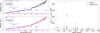 |
Fig. 9 Left: comparison between the best PPXF fit (blue) for an off-center spaxel of the F170LP data of Centaurus A (at a radius of 0.15″) of an uncorrected cube (top,gray) and one corrected using WICKED (bottom, red). The wiggles in the uncorrected cube bias the ability of PPXF to obtain a good velocity dispersion and cause the code to incorrectly identify emission lines (e.g., the [OIII] line ). The wiggles also impacts the LOSV, having a value in disagreement with the stellar rotation of V = 531 ± ΔV ≈ 25 km s−1 found in Cappellari et al. (2009). Right: absolute difference between the LOSV (black squares) and velocity dispersion (red triangles) for the binned spectra within 0.5″, comparing uncorrected and WICKED-cleaned spectra. The mean absolute difference for the LOSV (black dashed line) is ~181 km s−1, while for the velocity dispersion, it is ~104 km s−1. These values are ~17× and ~30× larger, respectively, than the propagated uncertainties of ~8 km s−1. |
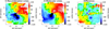 |
Fig. 10 Voronoi binned LOSV velocity maps for the Hydrogen recombination (left) and molecular lines (middle) for the F170LP NIRSpec observations of Centaurus A. The difference velocity map between the Hydrogen recombination and molecular lines (right panel) shows a velocity gradient along the radio-jet consistent with the finding of Neumayer et al. (2007). The maps are oriented such that North is up and east is to the left. |
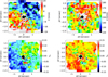 |
Fig. 11 Voronoi binned stellar velocity maps for the F170LP NIRSpec observations. The four panels show the line-of-sight velocity (V), the velocity dispersion (σ), and the first two Gaussian-Hermite moments (h3 and h4). The black diamonds show the five masked spaxels where a stellar fit is not possible due to the strong non-thermal AGN continuum. The orientation is the same as that in Figure 10. |
6 Conclusion
In this work we have presented a PYTHON tool called WICKED that can remove the PSF artifacts know as “wiggles” from the different NIRSpec gratings in the IFU mode. We have shown that spaxels in the data cube affected by these artifacts can be distinguished from the rest by analyzing their fast Fourier transform Section 3.2. WICKED removes the wiggles in the spectrum by taking advantage of the correlation between their frequency fλ and wavelength, as presented in Perna et al. (2023), but includes an important modification that leads to better removal of wiggles and preservation of the continuum shape and the emission or absorption lines in the spectrum. We performed different tests to the wiggle-free stellar spectrum of an A-star and an M-star to quantify the effectiveness of WICKED at identifying spaxels with wiggles versus Gaussian random noise and how well it preserves the EW of absorption lines, the shape of the spectrum, the line-of-sight velocity, and the velocity dispersion. The results of these tests are outlined in the following list:
The frequency of the wiggles in the spectrum depends on the brightness of the source and the dither pattern used during the observations. However, for a specific object, they have a defined range of frequencies that can be used to identify wiggles from the rest of the features in the spectrum using the fast Fourier transform. For the spectrum of the A-star used in our test, the mean amplitude of the Fourier spectrum at these frequencies is greater than the mean amplitude for the rest of the Fourier spectrum by a factor of ≥3σ up to a S/N of ~ 15, and ≥ 1σ at S/N of ~8;
We modeled the spectrum of flagged spaxels using a combination of an aperture spectrum, an annular spectrum, a power law, and a second-degree polynomial. These components were optimized by minimizing the chi-square of the fit at each spaxel. The two spectral templates help account for spatial variations in the cube and model different spectral features. Since many physical processes, especially at shorter wavelengths, can be represented by a power law, we included it to capture changes in the spectral shape that cannot be modeled using just the templates. The second-degree polynomial helps handle any remaining mismatches, such as common rises or drops at the spectrum edges or large bumps that sometimes show up (probably also PSF artifacts). We chose this approach instead of using a high-degree polynomial, as done in Perna et al. (2023), because high-degree polynomials can behave unpredictably and may mimic sinusoidal patterns, partially fit the wiggle amplitudes, and impact the ability to remove wiggles;
The EW of the spectrum corrected with WICKED for multiple lines shows a maximum relative difference of 5% from the true value across different S/N levels. On average, this is less than half the difference seen with the method by Perna et al. (2023) and four times smaller than the differences in the uncorrected spectrum. Differences in the overall spectral shape are up to 3.5 times smaller compared to the uncor-rected spectrum at S/N ≥ 200 and about 2.5 times smaller at S/N ≤ 100. Compared to the spectrum corrected with Perna et al. (2023), the difference is about 1.5 times smaller across all S/N levels. While the correction from Perna et al. (2023) leaves large regions of residual wiggles, especially at the spectrum edges, the spectrum corrected with WICKED only shows narrow “spiked” residuals around some absorption lines, which is consistent with the 5% difference mentioned earlier;
Wiggles significantly impact the ability to perform single-pixel level kinematics since they are mistaken as spectral features and thus produce artificially large velocity dispersions, and they can also be mistaken for broad emission lines. WICKED showed a better performance at recovering the true LOSV of the M-star used in our test as well as at reducing its uncertainty by a factor of about 50% compared to the method by Perna et al. (2023).
We also applied WICKED to correct for wiggles and analyze the nuclear gas and stellar kinematics of NGC 5128, or Centaurus A. This serves as a real example of the type of science that can be unlocked when removing these artifacts. We showed how the broad wiggles in the uncorrected F170LP cube of Centaurus A lead PPXF to wrongly identify emission lines in the spectrum and impacted the kinematics since PPXF would fit the wiggles as broad spectral features. The resulting gas and stellar kinematics of Centaurus A are in good agreement with previous works (Neumayer et al. 2007; Cappellari et al. 2009), showing a regular rotation for the molecular hydrogen and for the hydrogen recombination lines but with some distortion southwest of the center close to a knot in the radio jet (Neumayer et al. 2007). The stellar component shows a slow disk type of rotation that is counter-rotating by ~180º with respect to the molecular hydrogen. The stars also show an increase in velocity dispersion close to the center up to a radius of ~0.1″, where the strong non-thermal component in the spectrum completely vanishes the CO bandhead at 2.3 µm and impacts our ability to obtain a reliable fit. The first Gaussian-Hermite moment, h3, shows a clear anticorrelation with respect to the stellar LOSV, as expected for early-type galaxies (Krajnovic et al. 2008), with values similar to the SINFONI 100mas data in Cappellari et al. (2009) but with a clearer anticorrelation. The second Gaussian-Hermite moment, h4, shows a mean value of h4 = 0.04 and is quite symmetrical with respect to the center. The value of h4 is higher than reported in Cappellari et al. (2009) but within expectations for slow-rotator galaxies (Krajnovic et al. 2008). The higher h4 could also explain why we get on average a ≤10% higher velocity dispersion inside the 0.2″ than Cappellari et al. (2009). We believe that the disagreement is due to the template mismatch mentioned in Cappellari et al. (2009), which can impact the determination of h4 (Krajnović et al. 2008), and the superior sensitivity of JWST NIRSpec compared to their SINFONI data, which is why we also observe a clearer anticorrelation between the stellar LOSV and the h3 in our data.
The good agreement between the LOSV from the WICKED-cleaned spectrum and the aperture spectrum of the M-giant star J15395077 (Section 4.3), along with the overall consistency of NGC 5128’s gas and stellar kinematics with previous studies, suggests that the kinematics recovered from the WICKED-cleaned data cube closely represent the true values. Based on this, we find that the uncorrected spectra show significant differences in both LOSV and velocity dispersion compared to the WICKED-cleaned spectra, with discrepancies being on average ~30 times and ~12 times the typical propagated uncertainties, with the largest outlier reaching ~138 times and ~93 times, respectively (see Figure 9). These discrepancies highlight the importance of correcting for wiggles and that failing to do so can introduce substantial biases in kinematic measurements that far exceed expected uncertainties.
Wiggles significantly impact the possibility of doing single-pixel science across the different gratings of JWST NIRSpec in the IFU mode. The user-friendly aspects of WICKED combined with its capability to correct these artifacts across different signal-to-noise ratios presents a practical solution for the community to exploit the NIRSpec data and avoid spatial binning to remove wiggles. WICKED has already been applied to some datasets that will be presented in future works. We applied WICKED to clean the data for the “Revealing Low-Luminosity Active Galactic Nuclei” (ReveaLLAGN) sample, where we will present the stellar and gas kinematics in a future paper (Dumont et al. (in prep.)). It has also been used for cleaning the data for constructing the PSF model in Ohlson et al. (in prep.) and for cleaning the spectra of a couple of high-redshift Quasars in Wolf et al. (in prep.).
Data availability
The PYTHON package for WICKED is freely available and can be downloaded and PIP installed from the GITHUB repository https://github.com/antoinedumontneira/WiCKED.
Acknowledgements
LCH was supported by the National Science Foundation of China (11991052, 12233001), the National Key R&D Program of China (2022YFF0503401), and the China Manned Space Project (CMS-CSST-2021-A04, CMS-CSST-2021-A06.
Appendix A Characteristic frequencies of wiggles in Fourier space
In the Fourier transform of the wiggle spectrum for NIRSpec IFU data in high-resolution mode, we identified two distinct ranges of characteristic frequencies associated with the wiggles: a peak around 20 µm−1 and another around 40 µm−1. Interestingly, data from medium-resolution NIRSpec IFU observations show only the 20 µm−1 peak. This is illustrated in the right panel of Figure A.1, where we show the Fourier power spectra of the wiggle spectra from the brightest spaxel for all the data used in this work. The wiggle spectrum for each object was obtained by subtracting the brightest spectrum with a 3-spaxel radius aperture spectrum, as described in Section 4.
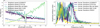 |
Fig. A.1 Brightest spaxels spectrum (left) and Fourier power spectra of the wiggle spectrum (right) for all the NIRSpec IFU data used in this work. The high-resolution datasets show two distinct peaks associated with wiggles at characteristic frequencies of ~20 µm−1 and ~40 µm−1. In contrast, medium-resolution data (e.g., P330-E, used in Law et al. (2023)) only show the lower-frequency component, indicating that the 40 µm−1 peak is unique to high-resolution modes. |
References
- Bianchin, M. U. V., Song, Y., et al. 2024, ApJ, 965, 103 [NASA ADS] [CrossRef] [Google Scholar]
- Böker, T., Arribas, S., Lützgendorf, N., et al. 2022, A&A, 661, A82 [NASA ADS] [CrossRef] [EDP Sciences] [Google Scholar]
- Bushouse, H., Eisenhamer, J., Dencheva, N., et al. 2024, https://doi.org/18.5281/zenodo.6984365 [Google Scholar]
- Cappellari, M. 2017, MNRAS, 466, 798 [Google Scholar]
- Cappellari, M., & Copin, Y. 2003, MNRAS, 342, 345 [Google Scholar]
- Cappellari, M., Neumayer, N., Reunanen, J., et al. 2009, MNRAS, 394, 660 [NASA ADS] [CrossRef] [Google Scholar]
- Cardelli, J. A., Clayton, G. C., & Mathis, J. S. 1989, ApJ, 345, 245 [Google Scholar]
- Davies, J. 2024, snowblind, 0.2.1. https://github.com/mpi-astronomy/snowblind [Google Scholar]
- de Graaff, A., Rix, H.-W., Carniani, S., et al. 2024, A&A, 684, A87 [NASA ADS] [CrossRef] [EDP Sciences] [Google Scholar]
- Doan, S., Satyapal, S., Matzko, W., et al. 2025, ApJ, 987, 99 [Google Scholar]
- Donnan, F. R., Rigopoulou, D., & García-Bernete, I. 2024, MNRAS, 532, L75 [NASA ADS] [CrossRef] [Google Scholar]
- Gardner, J. P., Mather, J. C., Abbott, R., et al. 2023, PASP, 135, 068001 [NASA ADS] [CrossRef] [Google Scholar]
- Husser, T. O., Wende-von Berg, S., Dreizler, S., et al. 2013, A&A, 553, A6 [NASA ADS] [CrossRef] [EDP Sciences] [Google Scholar]
- Jakobsen, P., Ferruit, P., Alves de Oliveira, C., et al. 2022, A&A, 661, A80 [NASA ADS] [CrossRef] [EDP Sciences] [Google Scholar]
- Krajnovic, D., Bacon, R., Cappellari, M., et al. 2008, MNRAS, 390, 93 [Google Scholar]
- Law, D. R. E., Morrison, J., Argyriou, I., et al. 2023, AJ, 166, 45 [NASA ADS] [CrossRef] [Google Scholar]
- Marconi, A., Pastorini, G., Pacini, F., et al. 2006, A&A, 448, 921 [NASA ADS] [CrossRef] [EDP Sciences] [Google Scholar]
- Neumayer, N. 2010, PASA, 27, 449 [NASA ADS] [CrossRef] [Google Scholar]
- Neumayer, N., Cappellari, M., Reunanen, J., et al. 2007, ApJ, 671, 1329 [NASA ADS] [CrossRef] [Google Scholar]
- Perna, M., Arribas, S., Marshall, M., et al. 2023, A&A, 679, A89 [NASA ADS] [CrossRef] [EDP Sciences] [Google Scholar]
- Rauscher, B. J. 2024, PASP, 136, 015001 [CrossRef] [Google Scholar]
- Riello, M., De Angeli, F., Evans, D. W., et al. 2021, A&A, 649, A3 [NASA ADS] [CrossRef] [EDP Sciences] [Google Scholar]
- Ruffio, J.-B., Perrin, M. D., Hoch, K. K. W., et al. 2024, AJ, 168, 73 [NASA ADS] [CrossRef] [Google Scholar]
- Silge, J. D., Gebhardt, K., Bergmann, M., & Richstone, D. 2005, AJ, 130, 406 [NASA ADS] [CrossRef] [Google Scholar]
- Smith, J. D. T., Armus, L., Dale, D. A., et al. 2007, PASP, 119, 1133 [NASA ADS] [CrossRef] [Google Scholar]
- Wright, G. S., Rieke, G. H., Glasse, A., et al. 2023, PASP, 135, 048003 [NASA ADS] [CrossRef] [Google Scholar]
Source: STScI JWST website
A JUPYTER NOTEBOOK template of our JWST pipeline sequence can be found at https://github.com/antoinedumontneira/NIRSpec-Ppipeline-Template
WICKED GitHub: https://github.com/antoinedumontneira/WiCKED
All Figures
|
Fig. 1 Top: brightest spaxel spectrum for the A-star J17571324 at different dither configurations. The horizontal bars show the wavelength for two wiggles in each NRS detector. Bottom: wiggle amplitude for the brightest spaxel of the same A-star J17571324 at different dither configurations. Having more dithers reduces the wiggle amplitude, but beyond eight dithers, the amplitude of the wiggles does not decrease significantly. |
| In the text | |
|
Fig. 2 Correction of the brightest spaxel in the F170LP cube of the A-star J1757132 using the CLEAN_CENTRAL_SPAXEL step in WICKED. The top panel shows the original spectrum (red) with prominent wiggles. The aperture (3-pixel radius) and annular integrated (3- to 5-pixel annular radius) spectra are displayed in gray and yellow, respectively, with the best-fit model shown in blue. Subtracting this smooth model from the single spaxel data produces the wiggle spectrum (middle panel, gray). WICKED identifies peaks and valleys in the wiggle spectrum (green crosses) and fits a wiggle model (red), which is subtracted to produce the final wiggle-free spectrum (bottom panel, red), pink vertical lines mark masked regions, while the yellow area highlights the gap between the NRS1 and NRS2 detectors. |
| In the text | |
|
Fig. 3 Example of a wiggle spectrum and its fast Fourier transform for the spectrum of J1757132. The fast Fourier transform is used in WICKED to flag spaxels in the data cube affected by wiggles. The built-in method PLOT_WIGGLE_FFT in WICKED allows for manual examination of the spectrum and its Fourier transform for a specific spaxel in the data cube. The left panel shows the wiggle spectrum created by subtracting the spectrum from the best-fit model. The right panel shows the Fourier transform of the wiggle spectrum. The solid fuchsia line represents the mean amplitude in the wiggle-dominated part of the spectrum (shaded red region). WICKED flags the spaxels by comparing the mean amplitude to the standard deviation (blue dashed line). If the data from the two NRS detectors are available, as in this case, WICKED determines which part of the spectrum shows the most prominent wiggles and bases the flagging on that part of the spectrum. |
| In the text | |
|
Fig. 4 Comparison of the spectrum of the A-star J1757132 (top, black) and the degraded spectrum (top, red) with the added wiggle model (green) at S/N ratios of 50, 15, and 8. Middle: Fourier spectra of (i) the degraded spectrum (solid, red), (ii) the wiggle model (green), (iii) the degraded spectrum without wiggles (black), and iv) the data corrected with WICKED (dashed, red). The horizontal lines mark the mean amplitude of the Fourier spectrum at frequencies dominated by wiggles and at larger frequencies. The Fourier ratio can effectively distinguish wiggles from noise down to a S/N ratio of ~8. Bottom: comparison of the input wiggle model (green) versus the recovered wiggle spectrum for the data cleaned with WICKED. |
| In the text | |
|
Fig. 5 Comparison of recovered EWs for two absorption lines present in the spectrum of the A-star (solid black line) J1757132. The bottom-left panel shows the profile of the LINE 1 for the original spectrum (solid black), the spectrum with wiggles (dashed), and the spectra corrected using WICKED (red) and with the code by Perna et al. (2023) (yellow). The line profile and EW are better recovered with WICKED than with the code by Perna et al. (2023), with the corrected spectrum having a less than 5% difference with the “true” value derived from the spectrum with no wiggles. For the uncorrected spectrum (gray), we observed EW differences exceeding the typical error (4%) in spectra with S/N as low as 50. |
| In the text | |
|
Fig. 6 Comparison of the mean difference flux with respect to the aperture spectrum of the A-star J175713. The black rectangles represent the minimum expected the flux difference at a given S/N ratio. The spectra corrected using WICKED (solid red) shows the smallest mean flux difference compared to the uncorrected spectrum (gray) and the spectrum clean using the method by Perna et al. (2023) (solid yellow) at all S/N. |
| In the text | |
|
Fig. 7 Comparison of WICKED and the code by Perna et al. (2023) at correcting for wiggles. The left panel shows the performance of both codes at recovering the wiggles model (shown in black in the bottom panel) added to the spectrum of the A-star J1757132 (solid black line). In the right panel we compare the performance of both codes at recovering the wiggles when the shape of the continuum is different from the integrated spectrum. We modified the spectrum by adding dust extinction with a value of AV = 20, using the Infrared-Optical relation by Cardelli et al. (1989). As shown WICKED is better at recovering the wiggle then the code by Perna et al. (2023), specially when the integrated spectrum is not a perfect model for the spectrum. |
| In the text | |
|
Fig. 8 Left: PPXF fits (blue) for the integrated spectrum (black) of the M-giant star J15395077, uncorrected brightest spaxel spectrum (gray), spectrum corrected with the code by Perna et al. (2023) (yellow), and spectrum corrected using WICKED (red). The FWHM aperture spectrum was degraded to match the S/N of the brightest spaxel of the cube. The best-fit LOSV and velocity dispersion for each spectrum are shown in the blue text boxes. We see that for an uncorrected spectrum it is not possible to obtain a reliable fit due to the wiggles, having a difference ~145 km s−1 with the LOSV of the integrated spectrum, three times larger than the estimated uncertainty. While, for both the spectrum corrected using WICKED and the code by Perna et al. (2023) a good fit can be achieved, with both being consistent within uncertainties with the LOSV of the integrated spectrum (wiggles-free). We note that using WICKED we obtain a best-fit value closer to the “true” value of 119.9 ± 2.7 for the integrated spectrum, and an uncertainty ~45% smaller than for the spectrum corrected with the code by Perna et al. (2023), which is probably due to the superior performance of WICKED at removing the wiggles. Right: residuals between each spectrum and the best fit. One can see that the residuals for the spectrum corrected using WICKED (red) are flat and mostly dominated by outliers left during the data reduction with the JWST pipeline, while for the spectrum corrected using the code by Perna et al. (2023) there are plenty of residual wiggles. |
| In the text | |
|
Fig. 9 Left: comparison between the best PPXF fit (blue) for an off-center spaxel of the F170LP data of Centaurus A (at a radius of 0.15″) of an uncorrected cube (top,gray) and one corrected using WICKED (bottom, red). The wiggles in the uncorrected cube bias the ability of PPXF to obtain a good velocity dispersion and cause the code to incorrectly identify emission lines (e.g., the [OIII] line ). The wiggles also impacts the LOSV, having a value in disagreement with the stellar rotation of V = 531 ± ΔV ≈ 25 km s−1 found in Cappellari et al. (2009). Right: absolute difference between the LOSV (black squares) and velocity dispersion (red triangles) for the binned spectra within 0.5″, comparing uncorrected and WICKED-cleaned spectra. The mean absolute difference for the LOSV (black dashed line) is ~181 km s−1, while for the velocity dispersion, it is ~104 km s−1. These values are ~17× and ~30× larger, respectively, than the propagated uncertainties of ~8 km s−1. |
| In the text | |
|
Fig. 10 Voronoi binned LOSV velocity maps for the Hydrogen recombination (left) and molecular lines (middle) for the F170LP NIRSpec observations of Centaurus A. The difference velocity map between the Hydrogen recombination and molecular lines (right panel) shows a velocity gradient along the radio-jet consistent with the finding of Neumayer et al. (2007). The maps are oriented such that North is up and east is to the left. |
| In the text | |
|
Fig. 11 Voronoi binned stellar velocity maps for the F170LP NIRSpec observations. The four panels show the line-of-sight velocity (V), the velocity dispersion (σ), and the first two Gaussian-Hermite moments (h3 and h4). The black diamonds show the five masked spaxels where a stellar fit is not possible due to the strong non-thermal AGN continuum. The orientation is the same as that in Figure 10. |
| In the text | |
|
Fig. A.1 Brightest spaxels spectrum (left) and Fourier power spectra of the wiggle spectrum (right) for all the NIRSpec IFU data used in this work. The high-resolution datasets show two distinct peaks associated with wiggles at characteristic frequencies of ~20 µm−1 and ~40 µm−1. In contrast, medium-resolution data (e.g., P330-E, used in Law et al. (2023)) only show the lower-frequency component, indicating that the 40 µm−1 peak is unique to high-resolution modes. |
| In the text | |
Current usage metrics show cumulative count of Article Views (full-text article views including HTML views, PDF and ePub downloads, according to the available data) and Abstracts Views on Vision4Press platform.
Data correspond to usage on the plateform after 2015. The current usage metrics is available 48-96 hours after online publication and is updated daily on week days.
Initial download of the metrics may take a while.