| Issue |
A&A
Volume 703, November 2025
|
|
|---|---|---|
| Article Number | A144 | |
| Number of page(s) | 25 | |
| Section | Cosmology (including clusters of galaxies) | |
| DOI | https://doi.org/10.1051/0004-6361/202554909 | |
| Published online | 14 November 2025 | |
KiDS-Legacy: Redshift distributions and their calibration
1
Ruhr University Bochum, Faculty of Physics and Astronomy, Astronomical Institute (AIRUB), German Centre for Cosmological Lensing, 44780 Bochum, Germany
2
Center for Theoretical Physics, Polish Academy of Sciences, al. Lotników 32/46, 02-668 Warsaw, Poland
3
Institute for Astronomy, University of Edinburgh, Royal Observatory, Blackford Hill, Edinburgh EH9 3HJ, UK
4
Department of Physics and Astronomy, University College London, Gower Street, London WC1E 6BT, UK
5
Department of Physics, University of Oxford, Denys Wilkinson Building, Keble Road, Oxford OX1 3RH, United Kingdom
6
Donostia International Physics Center, Manuel Lardizabal Ibilbidea, 4, 20018 Donostia, Gipuzkoa, Spain
7
Argelander-Institut für Astronomie, Universität Bonn, Auf dem Hügel 71, D-53121 Bonn, Germany
8
School of Mathematics, Statistics and Physics, Newcastle University, Herschel Building, NE1 7RU Newcastle-upon-Tyne, UK
9
Institute for Theoretical Physics, Utrecht University, Princetonplein 5, 3584CC Utrecht, The Netherlands
10
Leiden Observatory, Leiden University, P.O. Box 9513 2300RA Leiden, The Netherlands
11
Institut de Física d’Altes Energies (IFAE), The Barcelona Institute of Science and Technology, Campus UAB, 08193 Bellaterra (Barcelona), Spain
12
Centro de Investigaciones Energéticas, Medioambientales y Tecnológicas (CIEMAT), Av. Complutense 40, E-28040 Madrid, Spain
13
Institute of Cosmology & Gravitation, Dennis Sciama Building, University of Portsmouth, Portsmouth PO1 3FX, United Kingdom
14
Dipartimento di Fisica e Astronomia “Augusto Righi” – Alma Mater Studiorum Universitá di Bologna, via Piero Gobetti 93/2, 40129 Bologna, Italy
15
INAF-Osservatorio di Astrofisica e Scienza dello Spazio di Bologna, Via Piero Gobetti 93/3, 40129 Bologna, Italy
16
Universität Innsbruck, Institut für Astro- und Teilchenphysik, Technikerstr. 25/8, 6020 Innsbruck, Austria
17
The Oskar Klein Centre, Department of Physics, Stockholm University, AlbaNova University Centre, SE-106 91 Stockholm, Sweden
18
Imperial Centre for Inference and Cosmology (ICIC), Blackett Laboratory, Imperial College London, Prince Consort Road, London SW7 2AZ, UK
19
Zentrum für Astronomie, Universitatät Heidelberg, Philosophenweg 12, D-69120 Heidelberg, Germany; Institute for Theoretical Physics, Philosophenweg 16, D-69120 Heidelberg, Germany
20
Istituto Nazionale di Fisica Nucleare (INFN) - Sezione di Bologna, viale Berti Pichat 6/2, I-40127 Bologna, Italy
21
INAF – Osservatorio Astronomico di Padova, via dell’Osservatorio 5, 35122 Padova, Italy
22
Institute for Particle Physics and Astrophysics, ETH Zürich, Wolfgang-Pauli-Strasse 27, 8093 Zürich, Switzerland
23
Institute for Computational Cosmology, Ogden Centre for Fundament Physics – West, Department of Physics, Durham University, South Road, Durham DH1 3LE, UK
24
Centre for Extragalactic Astronomy, Ogden Centre for Fundament Physics – West, Department of Physics, Durham University, South Road, Durham DH1 3LE, UK
⋆ Corresponding author: This email address is being protected from spambots. You need JavaScript enabled to view it.
Received:
31
March
2025
Accepted:
26
August
2025
Abstract
We present the redshift calibration methodology and bias estimates for the cosmic shear analysis of the fifth and final data release (DR5) of the Kilo-Degree Survey (KiDS). KiDS-DR5 includes a greatly expanded compilation of calibrating spectra, drawn from 27 square degrees of dedicated optical and near-IR imaging taken over deep spectroscopic fields. The redshift distribution calibration leverages a range of new methods and updated simulations to produce the most precise N(z) bias estimates used by KiDS to date. Improvements to our colour-based redshift distribution measurement method using self-organising maps (SOMs) mean that we are able to use many more sources per tomographic bin for our cosmological analyses and better estimate the representation of our source sample given the available spec-z. We validated our colour-based redshift distribution estimates with spectroscopic cross-correlations (CCs). We find that improvements to our CC redshift distribution measurement methods mean that redshift distribution biases estimated between the SOM and CC methods are fully consistent on simulations, and the data calibration is consistent to better than 2σ in all tomographic bins.
Key words: galaxies: distances and redshifts / galaxies: photometry / cosmology: observations / gravitational lensing: weak / surveys
© The Authors 2025
 Open Access article, published by EDP Sciences, under the terms of the Creative Commons Attribution License (https://creativecommons.org/licenses/by/4.0), which permits unrestricted use, distribution, and reproduction in any medium, provided the original work is properly cited.
This article is published in open access under the Subscribe to Open model. This email address is being protected from spambots. You need JavaScript enabled to view it. to support open access publication.
1. Introduction
Wide-field imaging surveys with large mosaic CCD cameras and broadband optical and near-infrared (NIR) filters have entered a crucial era where significant fractions of the sky are currently being surveyed. The current generation called stage-III (Sevilla-Noarbe et al. 2021; Aihara et al. 2022; Wright et al. 2024) covers areas of more than a thousand square degrees and will soon be superseded by stage-IV surveys (Euclid Collaboration: Mellier et al. 2025; Ivezić et al. 2019) covering an order of magnitude larger areas at similar or greater depths. Perhaps the most crucial analysis step for virtually any application of these surveys is to add information about the radial distance of the very large number of objects (typically of the order of 107–109) reliably detected in such surveys. In the absence of spectroscopic redshifts for these huge samples of (mostly) galaxies, photometric redshifts (photo-z; for a recent review see Newman & Gruen 2022) based on broadband multi-colour photometry are used to solve this problem.
The estimation of these broadband photo-z for faint targets has been surprisingly stable over the past two decades (Hildebrandt et al. 2010). All stage-III surveys base their main scientific analyses still on template-fitting techniques developed more than 20 years ago (e.g. Benítez 2000). This reflects the maturity of these techniques and their close-to optimal use of information. Until the arrival of large, complete spectroscopic training sets down to the magnitude limits of these wide-field imaging surveys, which would enable highly precise and accurate photometric redshifts estimated via machine-learning techniques, this situation is unlikely to change (Newman et al. 2015).
These photo-z estimates of individual galaxies have well characterised error distributions with typical scatter of a few per cent around the true redshifts and equally a fraction of a few per cent of catastrophic outliers. These numbers have essentially remained unchanged for a long time. The main reason for this perceived stagnation in individual photo-z quality is the fact that this performance is not the limiting factor for the main science driver of such imaging surveys: weak gravitational lensing (WL).
The gravitational lensing effect is integrated along the line of sight and – in the case of WL – measured statistically by averaging over shear estimates of very large ensembles of galaxies. As such, a significant improvement in individual galaxy photo-z is not required. Instead, individual galaxy photo-z values are used only to divide the galaxy distribution into relatively broad, so-called tomographic bins (hundreds of Mpc comoving) along the line of sight.
It is the ensemble redshift distribution, N(z), that has rightly received most attention in WL measurements taken in the recent past as its accuracy is directly related to that of the cosmological parameters estimated from WL surveys. The increasing statistical power, hence, comes with a paralleled increase in the required accuracy of these N(z), most importantly expressed by their mean redshifts (Huterer et al. 2006). Higher-order moments of the N(z) are less important for cosmic shear but very relevant for other probes like galaxy clustering McLeod et al. (2017), Reischke (2024). Here, we concentrate on the former and leave the quantification of calibration uncertainties on higher-order moments of the N(z), such as width and skewness, to future work. For the current-generation stage-III surveys, the mean redshifts must be controlled at the percent level (Myles et al. 2021; Rau et al. 2023; Hildebrandt et al. 2021). Any larger bias in the redshifts would lead to a bias in the cosmological conclusions that would rival the statistical uncertainty. Calibration techniques are used to estimate the N(z), and simulations are employed to estimate residual biases, which can be used to re-calibrate the data. The uncertainty in this re-calibration is typically marginalised over in the cosmological inference.
The Kilo-Degree Survey (KiDS; Wright et al. 2024) is conducted with OmegaCam mounted at the Cassegrain focus of the European Southern Observatory VLT Survey Telescope (VST) on Paranal, Chile and complemented by the VISTA1 Kilo Degree Infrared Galaxy Survey (VIKING; Edge et al. 2013) observed from a neighbouring mountaintop. Together, these two surveys form a unique nine-band dataset covering the near-UV to NIR with (in terms of depth) well-matched high-resolution images over an area of ∼1350 deg2. With this extensive filter coverage, KiDS has the potential of estimating well-controlled photo-z down to its magnitude limit (r ∼ 24 for a typical WL source at a S/N of ∼10) and estimating accurate N(z) all the way to z ≲ 2, paving the way for similar multi-camera, optical+NIR efforts with, for example, Euclid.
While individual galaxy photo-z and their quality for the complete KiDS dataset are covered in the Data Release 5 (DR5) paper (Wright et al. 2024), here we describe the redshift calibration approach; that is, the estimation of the N(z), and their characterisation with simulations. This is the final paper in a list of publications that have developed the KiDS redshift calibration strategy (Hildebrandt et al. 2017, 2020, 2021; Wright et al. 2020a; van den Busch et al. 2020, 2022). Similar to previous efforts, we used two complementary techniques to estimate the N(z): one that is colour-based and another that is position-based. Both of these techniques leverage the power of spectroscopic surveys that overlap with KiDS or the newly compiled KiDZ dataset (i.e. the KiDS redshift calibration fields). The kinds of spectroscopic surveys used for the two techniques are quite different, though, which is highly beneficial for systematic robustness and independence of these methods.
The KiDS data, the KiDZ calibration fields, the calibrating spectroscopic surveys, and the tomographic binning approach are described in Sect. 2. The mock catalogues that mimic these different datasets are introduced in Sect. 3. In Sect. 4, the colour-based calibration technique via a self-organising map (SOM) projection of the 9D colour space is introduced. This is complemented by a description of the position-based calibration technique, also known as clustering redshifts (or dubbed CC for cross-correlation), in Sect. 5. The performance of these two approaches was evaluated on the simulated mock catalogues and is presented in Sect. 6. Results on the KiDS and KiDZ data are shown in Sect. 7, which are further discussed in Sect. 8 before we summarise in Sect. 9.
2. Data
This manuscript presents estimates of redshift distributions for the wide-field galaxy samples used in KiDS-Legacy. The KiDS-Legacy dataset is described at length in the KiDS DR5 data release document (Wright et al. 2024, hereafter W24). Here we summarise the pertinent information from the release including references to precise sections therein. We direct the interested reader to the data release document for detailed information regarding the data.
The fifth data release of KiDS consists of 1347 deg2 of weak lensing imaging data, and 27 deg2 of imaging covering deep spectroscopic calibration fields (with 4 deg2 of overlap). All data were observed with both VST and VISTA, yielding photometry in nine distinct photometric bandpasses (four optical and five NIR). Additionally, the entire wide and calibration footprint was observed twice in the i band, yielding two realisations and epochs of the photometry in this band. These realisations are kept separate in our analysis and are labelled i1 and i2 for distinction (the impact of the additional i-band measurements on our photo-z is shown in W24). This leads to a final dataset containing ten photometric bands, which are summarised in Table 1. Sources in these fields were extracted from the VST r-band imaging using SOURCE EXTRACTOR (Bertin & Arnouts 1996), within the Astro-WISE analysis environment (Valentijn et al. 2007; Begeman et al. 2013; McFarland et al. 2013), yeilding approximately 139 million unique sources.
Summary of relevant imaging data released in KiDS-DR5 (including KiDZ data).
All sources in KiDS-DR5 have photometric information measured in all available photometric bands. This photometric information was estimated through a form of matched aperture photometry that ensures consistent flux information is extracted from each source across the ten photometric bands, based on the optical r-band, and accounting for variations in the point spread function (PSF) per band. This forced photometry was performed with the Gaussian aperture and PSF code (GAaP; Kuijken 2008), and details of the implementation of GAaP in the context of KiDS-DR5 can be found in Sections 3.6 and 6 of W24.
After measurement of photometric information in all bands, the KiDS-DR5 sample was masked to include only unique sources that reside in areas of high-quality data in all bands. This masking process is described at length in Section 6.4 of W24 and results in 100 744 685 sources drawn from an effective area of 1014.013 deg2 (corresponding to an effective number density of 10.94 arcmin−2).
The lensing portion of the KiDS-DR5 sample was given the name KiDS-Legacy. As in previous KiDS analyses, the lensing sample contains per-source shape measurements and corresponding shape-measurement confidence weights estimated using the lensfit algorithm (Miller et al. 2007, 2013). These shapes were then calibrated with complex image simulations designed to emulate the properties of the KiDS-Legacy sample as closely as possible. A detailed description of these simulations is given in Li et al. (2023), and they are also summarised here in Sect. 3. The definition of the sample is provided in detail in Section 7.2 of W24, and involves a series of cuts in magnitude, colour, neighbour distance on-sky, and shape-measurement quality metrics. Additionally, Wright et al. (2025) found that masking of areas with higher astrometric noise was required to satisfy their cosmic shear B-mode null tests, leading to an additional masking of the survey footprint. The final KiDS-Legacy lensing sample is defined as the remaining 40 950 607 sources after these selections, drawn from 967.4 deg2 (corresponding to an effective number density of 8.81 arcmin−2).
2.1. Calibration datasets
The calibration sample used to estimate redshift distributions in KiDS-Legacy with the colour-based SOM method is drawn principally from the KiDZ sample described in Section 5 of W24. The KiDZ imaging were taken under the same observational conditions as the main KiDS and VIKING surveys and thus share the photometric properties of the wide-field dataset. The sample consists of 126 085 sources drawn from 22 spectroscopic samples and/or surveys, which have been compiled following a hierarchy that resolves internal and external duplicates in the datasets. The hierarchy ranks the constituents such that we kept spectra preferentially from the sample that is most likely to provide a reliable redshift. The details of this hierarchy and the homogenisation of the various redshift quality metrics are detailed in W24, and the resulting redshift distribution is shown in the top panel of Fig. 1.
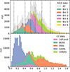 |
Fig. 1. Redshift distribution of the calibration data used for KiDS-Legacy. The top panel displays the full KiDZ data in grey and the proportion of it that enters each tomographic bin after calibrating the fiducial SOM, shown as a stacked histogram. The bin edges are indicated by the vertical dashed lines. The bottom panel shows the spectroscopic surveys used as calibration samples for the clustering redshift measurements (also stacked). |
The calibration sample for clustering redshifts used in KiDS-Legacy differs from the one described in W24. As opposed to previous work (van den Busch et al. 2020; Hildebrandt et al. 2021), we only included samples that cover multiple KiDS tiles and provide sufficient contiguous overlap with KiDS or KiDZ observations, namely: the 2-degree Field Lensing Survey (2dFLenS, Blake et al. 2016), Sloan Digital Sky Survey (SDSS, DR12) Baryon Osscilation Spectroscopic Survey (BOSS) low redshift (LOWZ) and constant mass (CMASS) samples (Alam et al. 2015), Galaxy and Mass Assembly (GAMA) DR4 (Driver et al. 2022), and the VIMOS Public Extragalactic Redshift Survey (VIPERS) PDR-2 (Scodeggio et al. 2018). We applied additional masking to ensure a consistent footprint between the KiDS-Legacy data, the spectroscopic data, and their provided spectroscopic random catalogues. We removed the relatively small overlap of 2dFLenS with the northern KiDS patch and limited the VIPERS dataset to a redshift range of 0.6 ≤ z < 1.18 to be consistent with the random catalogues and to mitigate the incompleteness from the colour sampling at z < 0.6 (Garilli et al. 2014). Finally, we added 109 381 recently released spectra from the Dark Energy Spectroscopic Instrument (DESI, DESI Collaboration 2016a,b) Early Data Release. Specifically, we used the designated clustering catalogues containing a subset of the luminous red galaxy (LRG) and emission line galaxy (ELG) samples (see Section 4.2 of DESI Collaboration 2024). This new set of calibration samples for the cross-correlation (CC) method (bottom panel of Fig. 1) covers a combined total of more than 80% of the KiDS-Legacy footprint (Fig. 2).
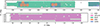 |
Fig. 2. Footprint of the spectroscopic surveys overlapping KiDS used for the clustering redshift measurements. VIPERS is exclusive to the KiDZ fields, which are not shown here. |
Table 2 details all datasets utilised for calibration in KiDS-Legacy. The table indicates samples that are used for our colour-based SOM redshift calibration (Sect. 4) and for our position-based clustering redshift calibration (Sect. 5). Their respective redshift distributions are shown in Fig. 1.
Spectroscopic redshift samples used for the KiDS-Legacy redshift calibration.
2.2. Weight assignment
One important distinction between the calibration fields and the wide-fields used for lensing is that the calibration fields lack the data-products required for lensfit shape estimation (specifically individual calibrated exposures; see W24). As such, sources in calibration fields that do not overlap with the wide-field data do not contain shape-measurement information, in particular the shape-measurement weights (see W24 for details about the imaging differences within the KiDZ fields). Since the shape weights correlate with the photometric observables, they present an additional selection that has to be taken into account in the SOM and the CC calibration.
Therefore, we replicated the lensfit weights in KiDZ using k-nearest neighbour matching. To each KiDZ galaxy we assigned the lensfit weight of a galaxy from KiDS-DR5 that is closest in r-band magnitude (MAG_AUTO), half-light radius (FLUX_RADIUS), GAAP major-to-minor axis ratio (Bgaper/Agaper), photometric redshift (Z_B), and average PSF size per tile (PSF_RAD). This matching process is therefore conditional on the KiDS and KiDZ data having consistent photometric properties, in particular in the r band (from which all but the photometric redshift metric are defined). Fortunately, the observation of the KiDZ data was taken with the same observational requirements as the main survey data, and as such the imaging are very well matched: for example, the distribution of KiDZ r-band seeing and magnitude limits (which drive the statistical properties of measured sizes and fluxes) are consistent with having been drawn randomly from the parent population of KiDS r-band seeing and magnitude limits, as computed using the two-sample Anderson & Darling (1954) test (p-values of 0.66 and 0.23, respectively).
To validate the accuracy of the matching process itself, we split the KiDS-Legacy wide-field sample into two halves (by splitting the survey at RA = 180 degrees) and inherited fake lensfit weights from one half onto the other. We then compared the inherited weights to those that were originally measured. For ease of interpretation, we rescaled the lensfit weights in this test to the range w ∈ [0, 1]. We found that the weight inheritance is robust, having a median residual between the real and synthetic weights of precisely zero, being driven by the vast majority of sources residing at a true weight of either zero or one, and being correctly assigned this limiting weight (thereby having precisely zero residual). The scatter in the weight residuals is similarly benign, at σ[wtrue − wfake] = 0.09 (a perfectly random assignment of fake weights produces a scatter of approximately 0.6). Hence, we conclude that the weight inheritance functions appropriately.
2.3. Tomographic binning
A central aspect of weak lensing tomography is the choice of tomographic binning. In all KiDS analyses to date, tomographic bins were defined using a set of cuts in photometric redshift (zB). For the initial KiDS cosmic shear analyses, based on optical data only, these cuts were constructed to have four bins of fixed width ΔzB = 0.2 between 0.1 < zB ≤ 0.9 (Hildebrandt et al. 2017)2. With the introduction of the VIKING NIR data and better high-z performance of the photometric redshifts, a fifth (higher redshift) tomographic bin was introduced, which used a width of ΔzB = 0.3 (0.9 < zB ≤ 1.2) (Hildebrandt et al. 2020). These selections resulted in tomographic bins that (for the last KiDS analysis, see Hildebrandt et al. 2021) contained between 2.8 million (bin one) and 8.1 million (bin three) sources.
This choice of tomography can, however, be shown to be sub-optimal for cosmic shear tomography signal-to-noise and figure-of-merit in typical applications. Sipp et al. (2021) advocate equipopulated bins as a better choice (over equidistant bins), and we opted to implement this form of tomography for KiDS-Legacy. Details of our chosen (six) tomographic bins, such as number densities and ellipticity dispersions, are provided in Table 3. It should be noted that the zB binning was chosen a priori based on the SKiLLS simulations (see Sect. 3 and Li et al. 2023). In combination with the discreteness of zB, this led to bins that are only approximately equipopulated in the KiDS-Legacy data.
Properties of the six KiDS-Legacy tomographic bins and the full source sample, using our fiducial redshift calibration procedure.
3. Simulations
Since the first cosmic shear analysis of KiDS (Hildebrandt et al. 2017), complex image simulations have been leveraged to calibrate shape-measurement biases (Fenech Conti et al. 2017). Subsequent analyses from Wright et al. (2020b) also utilised complex simulations to estimate informative priors on redshift distribution biases; however, these simulations were performed without an image layer. In KiDS-Legacy, we utilised the ‘SKiLLS’ suite of image simulations (Li et al. 2023) to, for the first time in KiDS, perform joint calibration of redshift distribution and shape-measurement bias parameters. Additionally, KiDS-Legacy also utilises an updated version of the MICE2 simulation (Fosalba et al. 2015a,b; Crocce et al. 2015; Carretero et al. 2015) presented in van den Busch et al. (2020) and utilised in Wright et al. (2020a). SKiLLS is a multiband image simulation based on the SURFS dark-matter simulation (Elahi et al. 2018) and Shark semi-analytic model (Lagos et al. 2018), and is constructed to match the observed multiband properties of KiDS-Legacy. SKiLLS is specifically designed to incorporate multi-wavelength imaging, realistic clustering, correlations between galaxies properties and environment, and redshift-dependent shear, thereby enabling the analysis and correction of higher-order effects in shape and redshift calibration. Conversely MICE2 is a simulated galaxy catalogue (i.e. without an image layer) derived from the MICE-Grand Challenge simulation, which we post-processed with an analytic photometry model. The two simulations were constructed to replicate the photometric properties of KiDS and VIKING data in each of the ugri1i2ZYJHKs bands as well as lensfit shape weights (beside other aspects such as shear, clustering, etc.).
There are two additional differences between SKiLLS and MICE2 that are worthy of comment. First, MICE2 covers an on-sky area of about 5000 deg2, whereas SKiLLS is limited to 108 deg2. Secondly, SKiLLS has a much larger redshift baseline (0.001 < z < 2.5) than MICE2, which is limited to 0.07 ≲ z ≲ 1.4 and therefore did not allow us to simulate the KiDS data in the sixth tomographic bin (or possible high-z tails of the other bins) with high fidelity. Additionally, as mentioned above, SKiLLS is used for joint shape-measurement calibration and redshift distribution bias estimation, which enables the correction of subtle unrecognised biases that correlate errors in shape-measurement and redshift distribution estimation (such as shear-based detection biases). Due to these differences, we relied on MICE2 to simulate our clustering redshift analysis (requiring the additional area), whereas SKiLLS was our primary simulation for the SOM calibration (covering the sixth bin). Nevertheless, the two simulations are useful where they overlap, since they give us additional redundancy and allowed us to test how our redshift estimates depend on the assumptions underlying both simulations.
3.1. SKiLLS
The multiband image-simulation based SKiLLS utilises imaging properties (limiting magnitudes, PSFs, etc.) sampled directly from the KiDS-1000 dataset (Kuijken et al. 2019), such that the observational parameters are representative of the parameter distributions therein. However, the base simulations tend to overproduce sources (relative to the data) at low-resolution and high signal-to-noise, leading to possible systematic biases in the recovery of shape calibration values, and which could also cause bias in redshift distribution estimates (as resolution and S/N are correlated with colour and redshift). Therefore, in order to optimise the similarity between simulations and data, Li et al. (2023) performed an a posteriori re-weighting of the simulated wide-field sources by comparing their abundance in a 2D space of shape-measurement S/N and source-resolution space to the KiDS wide-field data. In KiDS-Legacy we followed the methods of Li et al. (2023), and implemented a similar re-weighting scheme to construct our simulated calibration samples (see Sect. 3.3) and corresponding wide-field samples (see Sect. 3.3.2).
3.2. MICE2
For KiDS-Legacy we used an updated version of the KiDS-like MICE2 mocks that resembles DR5 and implements an improved analytic photometry model (Linke et al. 2025). We derived all the necessary calibration datasets from the underlying base simulation. Previous KiDS analyses have put considerable effort into analytically mimicking their observed properties as closely as possible (van den Busch et al. 2020), by reconstructing the samples’ selection functions (typically in colour, redshift, and/or derived properties such as stellar mass) in the simulation space. The documented spectroscopic success rate (as a function of redshift and magnitude) was similarly included where available. van den Busch et al. (2020) provide extensive demonstrations of the performance of this sample construction using the MICE2 simulation, which were used for the calibration of KiDS-1000. Generally speaking, it was difficult to faithfully reproduce the spec-z samples in the simulation space without ad hoc modifications to the original selection window, and as such they were defined with a modified selection window that reproduced the expected colour, redshift, and number density distributions seen in the data.
Similar to van den Busch et al. (2020), we constructed the wide-field calibration datasets such that they match observed spectroscopic data in sky coverage and relative overlap (e.g. between BOSS and GAMA), but additionally we decided to apply a stellar mask, which we constructed from the real KiDS-Legacy masks by tiling the MICE2 footprint. Since we used DESI and VIPERS data for the first time in a KiDS clustering redshift analysis, we implemented their respective selection functions for MICE2 similar to the existing ones for the GAMA, BOSS, and 2dFLenS samples of van den Busch et al. (2020). For details refer to Appendix A.
3.3. Simulating the KiDZ compilation
The KiDZ spectroscopic compilation is quite different from the wide area samples described above, since it covers only ∼20 deg2 on sky and extends to both significantly higher redshifts and fainter magnitudes. In previous work (Wright et al. 2020a; Hildebrandt et al. 2021) we elected to apply the existing deep field selection functions in MICE2 to many distinct lines of sight (appropriately sized for the spatial extent of the data calibration samples), to generate many realisations of the spec-z calibration samples in the simulation volume. This process produced N realisations of the spectroscopic compilation, each of which contained different realisations of underlying sample variance and photometric noise. Provided enough spatial realisations, the simulations were then assumed to span the range of possible calibration samples that could have been observed in the real Universe. Therefore, by calibrating our simulated wide-field sample with these realisations of the full calibration sample, we were able to estimate an average bias (and uncertainty) that captured the range of biases that would be seen under repeated observations of our calibration sample in different parts of the sky.
However, this is not directly the question of relevance for our cosmic shear analysis. Rather, the calibrating sample exhibits some particular joint distribution in redshift and colour, and we wish to identify the bias that is introduced to our analysis due to that specific joint distribution. In previous KiDS work using MICE2 (whose light cone covers a full octant of simulated sky), Wright et al. (2020a), Hildebrandt et al. (2021) used N = 100 lines of sight to estimate the uncertainty on the redshift calibration procedure. Should our observed calibration sample be an outlier in the distribution of all possible sample variance and photometric noise realisations, then there is only a small chance that such a realisation exists in a sample of 100 lines of sight. This is not formally a problem, but does decrease the interpretability of our cosmological posteriors somewhat.
Hence, in KiDS-Legacy we shifted the philosophy of our simulated analyses to focus on the issue of discerning the bias from the calibration sample that we actually have, rather than marginalising over the uncertainty from all possible calibration samples. This required a change in implementation of the construction of the calibration samples in the simulations. The new method of constructing realistic mock calibration samples (see Sect. 3.3.1) was applied to both SKiLLS and MICE.
3.3.1. Sample matching
As described in Sect. 3.3, the procedure for generating redshift calibration samples in simulations for KiDS-Legacy was updated to produce more accurate estimates of the redshift calibration bias present in the actual distributions of calibrating spectra available to us. This involved directly replicating the distribution of available calibrating spectra in multi-dimensional colour, magnitude, redshift, and photo-z space.
We performed the multi-dimensional matching using the galselect3 python module. The module takes two catalogues: a ‘candidate’ catalogue of potential sources, and a ‘target’ catalogue, which we wanted to reproduce. The module also takes a list of input features (such as colours and/or magnitudes), and a true-redshift designation for the two catalogues. In practice, we performed the matching in KiDS-Legacy using our ten-band magnitudes as the input features. With this information, the algorithm performs a brute-force search around each entry of the target catalogue to choose the best-matching candidate catalogue object. This brute-force search first involves truncating the candidate catalogue in a thin slice of true redshift around the target source redshift. This in effect forces the resulting matched catalogue to have the exact N(z) of the target catalogue, agnostic to the quality of the matched features. The feature match is then performed by computing the Euclidean distance (in the N-dimensional feature space) between all candidate objects and the target source. The best matching object is then chosen to be the candidate with the lowest Euclidean distance or (optionally) the candidate with the lowest Euclidean distance that has not previously been matched to a target source (i.e. allowing or not allowing candidate objects to be duplicated, respectively).
The algorithm therefore contains two primary options that are arbitrarily chosen by the user. Firstly the size of the window in true-redshift surrounding each target source that is used to define the possible candidate objects; and secondly features that are used to define the matching. In Sect. 6.1.3 we outline the influence of these options on the constructed calibration samples.
It should be noted that this algorithm, while yielding close-to perfectly matched redshift, colour, and magnitude distributions, does not necessarily also yield a sample with realistic clustering properties. Indeed, we believe that some of the samples constructed this way might have pathological clustering properties. Therefore, we decided to not use the matching algorithm for creating the wide-field samples used in the clustering redshift analysis on MICE2 and revert to the more traditional method of directly replicating the spectroscopic target selections there (see Sect. 3.2).
3.3.2. Matching to wide-field sources
One problem with the implementation of our matching approach for construction of the calibration samples in our simulations is that, if there are any systematic differences in the colour-redshift space between the simulations and the data, the matching algorithm will introduce a systematic discrepancy between the colour-redshift relation in the calibration- and wide-fields. To mitigate this possible effect, we implemented a similar matching algorithm between the data and simulation wide-field samples. However, this implementation cannot, of course, use true redshift as a basis (as in Sect. 3.3.1). Instead, we aimed to reproduce the wide-field sample in the simulations by matching sources, again by colour and magnitude, in discrete bins of photo-z, ensuring a perfect match of the photo-z distributions.
The algorithm proceeds simply by selecting all sources from both the wide-field samples on the data and simulations that reside at a particular (discrete) value of photo-z. These samples are then matched to one another using a k-nearest-neighbour method, and all simulation sources are tagged with the number of data-side sources that were most closely matched to them. This allowed us to construct frequency weights for all sources in the simulated wide-field sample, to more accurately reflect the observed distribution of sources in colour and photo-z. The resulting frequency-weighted wide-field sample is then used for calculation of redshift distributions and bias parameters.
4. Direct calibration with SOMs
For all cosmological analyses with KiDS since Hildebrandt et al. (2017), the fiducial estimation of redshift distributions and their calibration has been performed via some implementation of direct calibration (Lima et al. 2008). Wright et al. (2020a) presented an implementation of direct calibration using SOMs that has been utilised in all cosmological analyses with KiDS since 2020. In KiDS-Legacy, we also implemented a version of direct calibration with SOMs as our fiducial redshift estimation method, however, with a number of modifications not present in previous studies.
The calculation of redshift distributions for KiDS-Legacy was performed within the COSMOPIPE4 pipeline, described primarily in Wright et al. (2025) and used in an earlier form by Wright et al. (2020b) and van den Busch et al. (2022). Within COSMOPIPE, redshift distribution estimation was achieved using a sequence of processing functions. Crucial differences in the redshift distribution estimation procedure, compared to that implemented in previous analyses of KiDS, are: the use of one SOM per tomographic bin (Sect. 4.1), the use of gold weight rather than gold class (Sect. 4.2), and additional weighting on the calibration sample to account for prior-volume effects (Sect. 4.3).
4.1. Tomographic SOM construction
In their SOM implementation of direct calibration for KiDS, Wright et al. (2020a) trained a 101 × 101 cell SOM on the full KiDS+VIKING-450 (Wright et al. 2019) calibration sample of 25 373 sources, corresponding to roughly two calibrating sources per-cell on average. This SOM was then utilised to compute individual tomographic bin redshift distributions by subsetting the calibration sample (using the photometric redshift limits that define the tomographic bins) prior to the computation of direct calibration weights (DIR; see the beginning of their Section 4). Motivations for this choice are documented in Wright et al. (2020a), and focus (in particular) on systematic biases that occur when constructing N(z) using the full calibration sample rather than tomographically binned calibration samples. This process, however, resulted in a significant decrease in the number of sources that were calibrated by spectra in the wide-field sample (as much as a 30% reduction in the available number of sources in some tomographic bins). To circumvent this issue, the SOM cells were then merged using full-linkage hierarchical clustering to maximise coverage of the wide-field sample while maintaining a robust estimate of the redshift distribution. These merged groups of cells were then used in the computation of the DIR weights.
One caveat of the above procedure is that the number of cells assigned to regions of the colour-magnitude space dominated by the individual tomographic bins is non-uniform: tomographic bins with relatively fewer calibrating spectra receive fewer cells and less coverage in the combined SOM. This was not a problem for previous studies that used KiDS; however, in this study we introduced a new, higher redshift tomographic bin. This tomographic bin is both noisier (in terms of photometric properties) and has relatively fewer calibrating spectra than its lower redshift counterparts despite the increased number of spectroscopic calibration sources: 126 085, more than the previous KiDS calibration sample by a factor of roughly 5.
Therefore, in order to make optimal use of this larger calibration sample and accurately calibrate the higher-redshift tomographic bin, we opted for training one SOM per tomographic bin. This ensures that each tomographic bin contains the same number of cells in the training, and avoids the limitations that can be imposed by utilising a single SOM for calibration of the entire shear sample. The settings for the SOM training are summarised in Table 4. In particular, we note that the change to tomographic SOMs is accompanied by a reduction in the SOM size, from 101 × 101 to 51 × 51, to ensure similar cell population statistics when between tomographic and non-tomographic SOMs.
Fiducial parameters for SOM construction in KiDS-Legacy.
As a quantitative demonstration, we computed the tomographic-bin coverage statistics for a single 101 × 101 SOM trained in the same manner as for previous KiDS analyses. In such a SOM, the partitioning between individual tomographic bins is relatively good, with all tomographic bins covering 11 − 21% of cells (a perfect equipartition would correspond to approximately 15% after accounting for sources beyond the tomographic limits included in the training). Nonetheless, there is a factor of ∼2 difference in coverage between some bins, with bins four and five dominating (19.5% and 21.2% of cells, respectively). This is expected, as the unweighted N(z) of the calibration sample peaks in the region 0.6 < z < 1.1, where the bulk of bins four and five reside. In order to avoid this over-representation of the SOM manifold by bins four and five and give equal weight to all bins, we moved to individual SOMs for each bin.
4.2. Gold class versus gold weight
In the SOM redshift calibration implemented by Wright et al. (2020b), the authors introduced the ‘gold’ selection to the cosmic shear analyses. This selection flagged and removed sources that resided in parts of the colour-magnitude space that did not contain calibrating spectra. This gold-class selection improved the robustness of recovered cosmological constraints, by removing sensitivity of the recovered cosmology to systematic misrepresentation of calibrating spectra, which resulted in potential redshift biases, and which are a natural outcome of the wildly different selection functions between samples of galaxies from spectroscopic and wide-field imaging surveys.
In the establishment of the gold class, Wright et al. (2019) demonstrated that repeated construction of the gold class led to changes in the effective number density of sources (per tomographic bin) at the level of ≤3%, indicating that the gold selection was robust under repeated analysis. However, repeated end-to-end analyses of KiDS-1000 (within the new COSMOPIPE pipeline) showed more random noise in the recovered cosmological constraints than would naively be expected from a 3% change in the sample (with all other analysis aspects being equivalent to their KiDS-1000 counterparts). Investigation of this effect demonstrated an unrecognised feature of the gold selection. While the effective number density of sources per bin is stable under repeat analysis, the assignment of a gold flag to the sources themselves varies to a much higher degree. For example, repeated computation of the gold class will consistently classify 15% of sources as non-gold in a given tomographic bin, but precisely which 15% of sources are removed may vary from realisation to realisation. This has the effect of increasing the independence of the samples that are used in the end-to-end reruns of the cosmic shear data vector, and therefore increases the noise in estimated cosmological parameters between reruns. Testing on KiDS-1000, for example, demonstrated that the variation between shape-noise realisations implicit to the changing gold class could lead to variations in marginal constraints of S8 at the level of ≲0.5σ; much larger than one would expect from an apparent ∼3% change in the sample.
The cause of this effect is primarily photometric noise and the random nature of the SOM training, which combine to produce highly stochastic assignment of spectra to cells under any one training. While such run-to-run variation is not necessarily a problem a priori (the issue described above is rather with our assumption that the samples are consistent between trainings), we nonetheless sought an analysis alternative that reduced the sensitivity of our cosmic shear measurements to the training of an individual SOM. The simplest alternative is to perform the SOM training many times, and utilise the distribution of gold-class assignments as a weight in the final cosmological analysis: the ‘gold weight’.
We computed the gold weight by training Nrepl SOMs (either using the full sample or individual tomographic bin samples; see Sect. 4.1) and calculated the gold class of all sources per bin for each of these SOMs. The gold weight was then defined as
 (1)
(1)
where the gi, j are the 0/1 gold classifications assigned to each source i under realisation j of the SOM training. Using this gold weight, we were able to construct N(z) that are less sensitive to the randomness of any single gold-class assignment, and to construct data-vectors that are more consistent under end-to-end reruns of the analysis pipeline. This has the primary benefit of creating less statistical noise in repeated analyses of KiDS, leading to a more robust legacy data product. An additional benefit of gold-weighting is that it eliminates the requirement for the hierarchical clustering of SOM cells, which was performed by Wright et al. (2019) to increase the fraction of positive gold-class assignments for wide-field sources. Figure 3 demonstrates the benefit of gold weight over gold class visually. The gold-class definition is highly stochastic, as cells that are classed as gold in a single realisation are assigned a wide range of gold weights after many realisations.
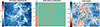 |
Fig. 3. Comparison between gold-class and gold-weight definitions. Here, a SOM trained on tomographic bin one in our SKiLLS simulation is coloured by the true mean redshift of each cell (left), the gold-class definition of each cell under a single realisation (centre), and the gold weight of each cell after ten realisations. In the gold-weight panel, the cells, which are assigned a (highly stochastic) zero gold class in our single realisation, are highlighted with an orange border. These cells are assigned a wide range of final gold-weights, highlighting the stochasticity of the gold-class definition and the superiority of the gold-weights. In each colour bar, the PDF of cell values is shown. |
The distribution of gold weights computed for our fiducial simulations in KiDS-Legacy are shown in Figure 4. It is apparent from the figure that the gold weight per source varies strongly per tomographic bin; however, the behaviour is qualitatively similar in the most relevant aspects: all bins have a peak in their gold-weight probability distribution function (PDF) at unity (implying that sources are typically consistently classed as gold under realisations of the SOM), and very few sources have a gold weight of zero (suggesting that it is rare for sources to be consistently unrepresented in the calibration compilation under realisations of the SOM). This result is consistent with the conclusion that the variability in gold assignment is driven by photometric noise.
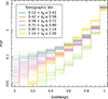 |
Fig. 4. Distributions of gold weight per tomographic bin for our fiducial SKiLLS simulations. Individual lines show the scatter in the gold-weight PDFs under different realisations of our spectroscopic calibration samples. The tomographic bins show qualitatively similar behaviour: many sources are consistently classed as gold under all realisations of the SOM (wgold = 1), and very few sources are consistently classed as not-gold under all realisations (wgold = 0). |
4.3. Prior redshift weight
The SOM implementation of the direct calibration method is designed to perform two primary tasks: re-weight the colour space of the calibration sample to better represent the wide-field sample, and flag wide-field sources for removal where this correction is not possible (i.e. the gold-weighting). These corrections assume, however, that the probability distribution of redshift at a given colour in the calibration and wide-field samples are identical. Such an assumption is easily violated in the process of spectroscopic redshift acquisition, where two galaxies with different redshift but the same broadband colours (i.e. those with colour-redshift degeneracy) have different spectroscopic redshift success rates (e.g. one galaxy shows the [OII] doublet in the optical and the other does not). Such a selection in the successful acquisition of spectroscopic redshifts has been shown to lead to pathological biases in vanilla direct calibration implementations (Hartley et al. 2020).
Even more simply, however, this assumption is also easily violated when the samples are constructed from vastly different selection functions (e.g. Gruen & Brimioulle 2017). For example, two simple magnitude-limited samples constructed from different magnitude limits will probe different redshift baselines. If the deeper sample has access to galaxies that are colour-degenerate with galaxies in the shallower window, then the redshift distribution at fixed colour will be unimodal for the shallow sample and multi-modal for the deeper sample.
Correcting for this effect is complicated, as it requires one to know the distribution of redshift for the target sample of galaxies (which is our desired end-product of the SOM calibration process). In KiDS-Legacy, we performed a first order correction using an a priori estimate of the wide-field sample redshift distributions (see below) and removed significant differences between this wide-field estimate and the (known) redshift distribution of the calibration sample.
To perform this correction, we required an estimate of the true redshift distribution of the cosmic shear wide-field galaxy sample. To this end we began by constructing an analytic expression for the redshift distribution of an arbitrary magnitude-limited sample. Using the raw 108 deg2 SURFS-Shark light cone (see Sect. 3), which contains noiseless SDSS and VIKING fluxes, we constructed samples of galaxies cut to various magnitude limits in a range of photometric bands. We then fitted each of the resulting galaxy samples with the function:
 (2)
(2)
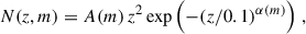
where A and α are free parameters. We then modelled A(m) and α(m) with a fourth-order polynomial. This allowed us to construct an analytic redshift distribution for a sample of galaxies that is magnitude-limited (in true flux) between the 18th and 27th magnitude in any band from u to Z. An example showing the estimated model parameters, the polynomial fits, and the resulting analytic N(z) is given in Fig. 5.
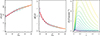 |
Fig. 5. Model parameters and the resulting analytic N(z) for samples defined as magnitude-limited (in the r band) from our noiseless SURFS+Shark light cone. The left and centre panels show the free parameters from Eq. (2), as a function of the r-band magnitude limit, including polynomial fits. The right panel shows the analytically estimated N(z) for each of the models parameters in the other two panels. |
We subsequently constructed prior volume corrective weights for the KiDS-Legacy calibration sample using this analytic prescription. To do this we first selected a magnitude-limited sample that we found closely mimics (in terms of the redshift distribution) the expected true selection function of our wide-field shear dataset; a process that is complicated by the various complex lensing selections (and shape weights) that are applied to the wide field lensing sample of galaxies.
We chose to use a sample that is magnitude-limited in the r band, at 20 ≤ r ≤ 23.5. The bright-end magnitude limit was chosen because of the selection performed by lensfit that rejects galaxies at r < 20. The faint-end limit was chosen due to the lensing weights returned by lensfit, which are strongly magnitude-dependent: at r ≈ 23.5 the lensing weight is roughly half its maximum. With our analytic estimate of the wide-field sample redshift distribution, we then defined the corrective prior volume weights as the ratio of the redshift distribution PDFs Pw(z)/Pc(z), where w and c refer to the analytic wide-field sample and the data calibration sample, respectively. The impact of the prior volume weights on the total N(z) of the spectroscopic compilation, and also for an example tomographic bin, are shown in Fig. 6. The figures show the distributions both before and after SOM weighting, and when including our simulation-informed estimates of N(z) bias (see Sect. 6). It is clear from the figure that the prior volume weights have a systematic effect on the relative weight of individual calibrating sources as a function of redshift and, perhaps more importantly, that this manifests as a shift in the entire pre-weighting N(z) for some tomographic bins. After weighting by the SOM, however, the differences are less pronounced, indicating that some of the difference between the redshift distributions is absorbed by the colour-cell DIR weights (thanks to the colour-redshift relation). Finally, after incorporation of our simulation N(z) bias estimates the differences are reduced even further (see Sects. 4.4 and 6), demonstrating the importance of having realistic simulations to correct for methodological bias in N(z) estimation and calibration.
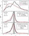 |
Fig. 6. Impact of prior-volume weights on the (pre-SOM) N(z) of the full spectroscopic compilation (upper panel), and on those galaxies in the compilation that end up in tomographic bin three both prior to the SOM re-weighting (middle panel) and after the SOM re-weighting (bottom panel). The systematic effect that the prior weight imparts on the tomographic bin is particularly clear prior to re-weighting by the SOM to match the wide-field sample but is somewhat diluted by the SOM re-weighting process. Nonetheless, there is a residual difference after the SOM re-weighting in the bottom panel. This difference is exacerbated if one does not have high quality image simulations to calibrate the underlying N(z) bias (dashed lines in the bottom figure; discussed further in Sect. 6), as the non-prior weighted N(z) estimate contains a significant systematic bias (⟨δz⟩≈0.03), whereas the prior weighted N(z) estimate has no bias (⟨δz⟩≈0.004). |
4.4. Redshift distribution bias estimation
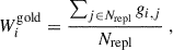
Calibration of the redshift estimation process (specifically the derivation of tomographic bin redshift bias parameters) in KiDS-Legacy was performed by implementing the redshift distribution estimation pipeline on our various simulated datasets, which are designed to mimic the observed data as accurately as possible. With the estimated redshift distributions and the known true (weighted) redshift distribution of the source samples, we then computed the bias of each estimated redshift distribution as
 (3)
(3)
where μz is the (shape- and gold-) weighted mean true redshift of the wide-field sample, and  is the estimated mean redshift of the wide-field sample, computed directly from our weighted calibration sample5. We typically perform this measurement using many realisations of the calibration samples, which produces many estimates of
  (and, because of the gold selection or weighting, possibly many different μz). Our final quoted biases are the arithmetic means of the biases estimated per tomographic bin and pipeline setup (⟨δz⟩). The population scatter of the biases in these realisations is also a relevant consideration, and is quoted as σδz. We note in particular that these uncertainties are smaller than those in previous KiDS analyses, due to the change in simulation philosophy described in Sect. 3.3.
5. Clustering redshift methodology
As a complementary approach to test and validate the SOM N(z) we used clustering redshifts (e.g. Newman 2008) following previous KiDS work (Hildebrandt et al. 2017, 2020, 2021; Morrison et al. 2017; van den Busch et al. 2020). The DR5 analysis presented here is an evolution of these previous studies, adding more area for the measurements of the CCs and, more importantly, expanding the suite of external spectroscopic surveys used for the calibration. The dedicated KiDZ data allowed us to measure CCs with VIPERS, providing additional constraints in the range 0.6 < z ≲ 1.2. Recently, the DESI Early Data Release provided a number of additional galaxies with spectroscopic redshift estimates extending to even higher redshifts and overlapping with the KiDS main survey area in six rosette-shaped DESI pointings. Together these advances allowed us to validate the SOM N(z) for the first five tomographic bins (bin six is only partly covered) without referring to deep, pencil-beam surveys (as we still had to do in Hildebrandt et al. 2021), significantly decoupling the clustering redshift from the SOM approach in terms of calibration data. One caveat, though, is VIPERS, which is used for both CCs and SOM N(z) calibration. However we found that the overall contribution of VIPERS both SOM and CC N(z) calibrations is subdominant (see Sect. 5.2) and so the independence of the methods is maintained.
5.1. Correlation measurements
KiDS clustering redshifts are estimated with the versatile, public code yet_another_wizz6 (YAW, van den Busch et al. 2020), which is based on concepts already introduced by Schmidt et al. (2013) and Morrison et al. (2017). In particular we used the publicly available version 2.6.0, which differs from the versions used in previous publications (e.g. Hildebrandt et al. 2021; Naidoo et al. 2023) in a few ways.
The code now generates N spatial regions per calibration sample based on k-means clustering of sky coordinates (e.g. using random catalogues) instead of splitting the data into the N individual square-degree pointings spanned by each dataset. These regions are used to estimate the data covariance via a spatial jackknife (previously using bootstrap). This empirical data covariance was tested against analytical models for the covariance matrix based on halo occupation distributions and a halo model approach for a different calibration dataset derived from MICE2. While there is good general agreement between the features of the empirical and the analytical covariance, we opt to rely on the jackknife method due to the highly non-linear regime of the clustering measurements, possible uncertainties in the halo occupation distribution, and non-Limber effects in the connected non-Gaussian terms (for details we refer to Section 9.2 of Reischke et al. 2025). Regardless, the agreement with the analytic covariance serves as a good cross-check for the empirical jackknife covariance that we use throughout the clustering redshift analysis.
In addition to the above, the code now measures pair counts across the boundaries of these spatial regions7 and the Landy-Szalay estimator (Landy & Szalay 1993) is used for all auto-correlation measurements. Finally, in the case of the CCs, which use the Davis & Peebles (1983) estimator, only one random catalogue is needed. Hence, one can decide whether to use a random catalogue for the spectroscopic or KiDS data. We decided to use random catalogues for the spectroscopic data instead of the KiDS data in those cases, since most of the spectroscopic surveys provide well-established random catalogues that take into account and correct for a lot of systematic effects.
5.2. Fiducial analysis setup
We measured angular correlations in a single bin of fixed transverse physical separation between 0.5 < r ≤ 1.5 Mpc in 32 linearly spaced redshift bins in the range 0.05 ≤ z < 1.68. For MICE2, the upper redshift limit is reduced to zmax = 1.4.
One of the main goals of any clustering-redshifts setup is to suppress and mitigate the redshift evolution of the galaxy bias of the calibration data and the target wide-field dataset. Following the notation of van den Busch et al. (2020), these biases can, under certain assumptions, be expressed in terms of the amplitudes of the angular autocorrelation functions of our spectroscopic reference sample, wss(z), and the wide-field photometric sample, wpp(z). Then, the true (unknown) redshift distribution can be written as
 (4)
(4)
where wsp(z) is the CC amplitude between the spectroscopic and photometric samples, Δz is the bin width of the CC measurements, and NCC(z) denotes our estimated N(z) from the CC method.
In our fiducial analysis we chose to only correct for the calibration data bias; that is, we effectively measure the numerator of the right-hand side of Eq. (4). This is achieved by measuring the angular auto-correlation function of the calibration sample in the same redshift and distance bins as the CC function. This approach has been shown to successfully remove the redshift evolution of the galaxy bias of that sample. However, a similar treatment is not possible for the KiDS-Legacy source samples. The impact of the unknown galaxy bias of that sample data is partly mitigated by the fact that we bin the data tomographically (Schmidt et al. 2013), and it has been shown previously to be sufficiently small that we can neglect it in our following analysis (see e.g. Hildebrandt et al. 2021; van den Busch et al. 2020).
Finally, we produced a joint redshift estimate from all five calibration samples for which we measured the correlation functions independently. We obtained this final estimate by computing the inverse-variance weighted average of the bias-corrected correlation measurements of all reference samples. This produces an optimal redshift estimate that reflects the redshift-dependent relative contribution of each correlation measurement to the overall redshift estimate and accounts for the different statistical power each calibration sample has at any given redshift (Fig. 7). In general, the joint CCs were found to be dominated by BOSS, GAMA, and 2dFLenS at z ≲ 0.7 and by DESI at high redshifts, whereas VIPERS had an overall small contribution due to its limited area and number density.
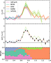 |
Fig. 7. Example of the inverse-variance weighted combination of CCs computed from the fourth tomographic bin of MICE2. The top panel shows the individual measurements from each calibration sample, the middle panel the weighted average, and the bottom panel the relative weight of each sample as a function of redshift. |
5.3. Adaptation of signal-to-noise in MICE2
When comparing the S/N in the measured CCs on the between the data (from KiDS and KiDZ) and MICE2, we find that the noise level in the simulation is typically much smaller in most redshift bins, especially in the sixth tomographic bin (see top panel of Fig. 8). The reason for this difference is not entirely clear. Possible reasons could be differences in the selection functions applied to MICE2 for both the calibration and KiDS-Legacy data, as compared to the real data. There may also be a difference in the overall clustering amplitude found in the data and the simulations, especially on small scales. Additionally, the key difference between the data and MICE2 is that the mock photometry is perfectly uniform such that the effects of variable depth (Heydenreich et al. 2020) are not present in the simulation. Finally, there may be other systematic effects in the data for which our MICE2 data does not account, for example, related to fibre-collisions in the spectroscopic reference sample, for which DESI (for example) require special pair-weights (Bianchi et al. 2018) that we currently cannot integrate into our correlation estimator.
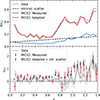 |
Fig. 8. One realisation of the CC measurements from MICE2 in the sixth tomographic bin after noise adaptation (Sect. 5.3) and the addition of intrinsic scatter (Sect 5.4). The top panel compares only the uncertainties of NCC(z) from the data (grey) and MICE2 before (blue) and after adaptation (red). The dashed black line indicates the fitted intrinsic scatter from the measurements on the data (f = 0.14 ± 0.04; see Eq. 6). The bottom panel shows the measured NCC(z) from MICE2 (blue points) compared to the data (grey line). The red data points represent the MICE2 measurements after adapting the noise (up-scaling errors and perturbing values) and adding the intrinsic scatter (only perturbing valu-es) obtained from the data. |
Since there was no clear explanation for this difference between data and simulation, we opted to adapt the measurements on the mocks by adding additional Gaussian noise to the values and inflating the error bars such that they match the data. We computed the right amount of noise required from the difference between the covariances of the inverse-variance-combined measurements of data and mock. Figure 8 shows a comparison of the original measurements in MICE2 and how the adapted version compares to the data measurements in the sixth tomographic bin.
5.4. Modelling of the measurements
A long-standing issue within clustering redshift measurements is that the measured correlation functions are, by definition, not probability densities and must therefore be modelled in some way. A number of different approaches (e.g. Johnson et al. 2017; Stölzner et al. 2021; Gatti et al. 2022; Naidoo et al. 2023) have been implemented to mitigate the frequently arising negative correlation amplitudes, as they represent only a noisy realisation of the underlying redshift distribution. Given the dominant sensitivity of cosmic shear to the mean redshifts of the tomographic bins, we opted for simplicity here and use the SOM N(z) as a model that we fit to the CC data via a simple shift in redshift, Dz, and a free normalisation9, A, such that
 (5)
(5)
This approach, however, can be quite sensitive to single data points with small variance, which can be aggravated in case of mismatches between the shape of the CCs and the model N(z). This is of particular importance since there seems to be some additional intrinsic scatter in the data CCs that exceeds the variance that one expects given the uncertainties of the measurements. This intrinsic scatter is most obvious in bins five and six and, in particular, at high redshifts.
Observational systematics might introduce such erroneous additional correlations and could be reduced in future work by using organised random catalogues (Yan et al. 2025). Here, we opted for a simpler empirical correction and extended our fit model with an additive error term f (1 + z) with free amplitude, f, such that the combined uncertainty s for each measurement was
 (6)
(6)
We integrated this error term into our likelihood and marginalised over f when determining the shift parameters Dz and the amplitudes A.
This process of measuring and modelling clustering redshifts with a reference N(z) was tested on the MICE2 mocks, where we could additionally use the true redshift distribution as a fit model in Eq. (5). This allowed us to verify the robustness of, and determine any biases inherent to, our methodology. A key difference with respect to the data, however, is that the additional intrinsic scatter, parameterised by the f-term, is not present in MICE2. We therefore determined f on the data by fitting each tomographic bin and added the expected intrinsic scatter to the mock measurements. We perturbed the data points (but not their uncertainties, which were already adapted via the method described in Sect. 5.3) with Gaussian noise with a variance of f2 (1 + z)2, which is also included in the example shown in Fig. 8. Since we must avoid biases that may arise from a certain random realisation of the added scatter, we always created 100 realisations, fit each of them independently, and computed the mean and variance of Dz from all realisations.
6. Simulation results
In this section, we present the results of the redshift distribution estimation from our simulated galaxy samples. In Sect. 6.1 we detail the redshift distributions and bias parameters estimated using our SOM algorithm. In Sect. 6.2 the redshift distributions and bias parameters estimated using the CC method are shown. Within these sections, we cover the sensitivity tests that were performed to determine the robustness of the methods.
6.1. SOM redshift distributions
Table 5 summarises the results of our SOM redshift distribution calibration using our various simulations. The table presents multiple statistics, which we outline here.  is the average of the estimated redshift distribution first moments (i.e. means) under realisations of the calibration sample (see Sect. 3). ⟨δz, 0⟩ is the average bias in the first moments prior to any re-weighting by the SOM, under realisations of the calibration sample, relative to the true weighted redshift distribution of the lensing sample (which is naturally unknowable for real data). ⟨δz⟩ is the average bias in the first moments after re-weighting by the SOM. σδz is the standard deviation of the distribution of biases after re-weighting by the SOM. Finally, Δ⟨δz⟩=⟨δz⟩−⟨δz⟩ref is the difference of the average biases, after re-weighting by the SOM, between a given scenario and a reference/fiducial scenario.
Redshift distribution estimates from simulations.
6.1.1. [A]: Fiducial calibration
We computed the N(z) and bias parameters for our fiducial SOM redshift calibration methodology and parameter set (Table 4), and subsequently compared alternative analyses (such as sensitivity tests) to these fiducial results. The results of these sensitivity tests were then folded into our analysis in one of two ways. For tests that are expected to have no impact on the redshift distributions (such as perturbations to ad hoc parameters of the simulation construction), we folded differences in recovered N(z) into our systematic error budget. For tests that are expected to have some systematic (possibly non-negligible) impact on the redshift distributions (such as alternate sample weighting), we utilised the resulting N(z) and bias parameters for use in full end-to-end reruns of the KiDS-Legacy cosmology, and presented these results as alternative cosmological constraints in Wright et al. (2025). This is because the differences in biases that arise from the latter type of analyses are not indicative of systematic effects in the methodology: rather the samples underlying the analyses have become systematicallydifferent.
Resulting N(z) for our fiducial SOM redshift calibration methodology are provided in Fig. 9. The redshift distributions are well constrained to the tomographic bin limits for all six tomographic bins used in KiDS-Legacy, with the third tomographic bin showing the largest outlier population (an extended tail to low redshifts) and the sixth tomographic bin showing a bias to somewhat lower redshifts than targeted by the photo-z cuts. The figure shows the full range of redshift distributions estimated with realisations of the calibration sample as a filled polygon. Overlaid is the true target N(z), which is also shown as a polygon but which has, in effect, vanishingly small area. The figure demonstrates the consistency of the estimated and true redshift distributions: in every bin, our estimated N(z) are able to successfully capture the full complexity of the source redshift distributions with accuracy and precision.
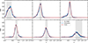 |
Fig. 9. Redshift distributions for the fiducial SOM calibration methodology, computed using the SKiLLS simulations. The ensemble of blue polygons show the N(z) constructed with different realisations of the calibration sample. Redshift distributions include the new gold-weighting for the wide-field sample, and prior volume weighting and shape-measurement weights for the calibration samples. |
Our fiducial redshift distributions and biases are somewhat different to those presented in previous KiDS analyses, such as Wright et al. (2020a). In particular, the uncertainties on the bias parameters are an order of magnitude smaller than in previous work, down from σΔz ≈ 0.01 to σΔz ≈ 0.001. This reduction is attributable primarily to the use of our matching algorithm, which forces the calibration sample redshift distribution to be identical under all realisations (that is, equal to the observed redshift distribution), regardless of the underlying large-scale structure. These fiducial uncertainties form our base uncertainty for the SOM calibration method, which are then increased as needed to encompass the systematic uncertainties determined for the method in the sections below.
Finally, we note again that, compared to previous SOM redshift calibration work within KiDS (see e.g. Wright et al. 2020a; Hildebrandt et al. 2021; van den Busch et al. 2022), the redshift calibration process here utilises different tomographic binning and a much larger spectroscopic calibration sample. Furthermore, we implement various weights and selections on the calibration side not previously implemented in KiDS. This makes direct comparison between our fiducial results and results presented in previous KiDS work difficult; it would be inappropriate, for example, to apply calibrations presented here to previous work with KiDS (without redoing the redshift calibration entirely).
6.1.2. [B]: Single shear realisation
Our fiducial analysis used the full SKiLLS simulation set, including eight realisations of the simulated photometry catalogues that were generated by applying four uniform shears and two position angle rotations to all sources in the 108 deg2 of simulated sky. These realisations are useful as each has an independent realisation of photometric noise, allowing us to increase the effective size of our simulated catalogue by a factor of 8. This does not, however, reduce the sample variance contribution to the analysis, as all photometric realisations are drawn from the same underlying large-scale structures.
The motivation for the use of all shear realisations in the fiducial pipeline is a practical one: we require the shear realisations for shape calibration, and all sources must be appropriately gold-weighted. However, using the multiple photometric realisations considerably increases the runtime of our calibration. Therefore, in the interest of speed and reducing unnecessary power consumption, we only utilised a single shear realisation for much of the redshift calibration testing presented here.
In that respect, we first verified that the results that we find for our fiducial redshift calibration process are unchanged under reduction of the number of sources available for calibration testing. These results are presented in Table 5: we found that the use of a single shear realisation produces bias estimates that are consistent with the fiducial case to better than |Δ⟨δz⟩| = 0.0012 in all bins. Furthermore, the scatter of the calibrated biases is always consistent between the single and fiducial shear runs, with the exceptions that the scatter is increased in bin one and decreased in bin six. However, as the absolute size of the scatter is still relatively small, we conclude that there is unlikely to be a systematic bias introduced in our testing process by using a single shear realisation in redshift calibration testing.
6.1.3. [C]: Matching algorithm validation
We validated the robustness of our calibration to the ad hoc matching algorithm parameters (described in Sect. 3.3.1) byconstructing multiple realisations of the calibration sample using perturbations on the fiducial choices. We then propagated these modified calibration samples through the redshift calibration pipeline and compared the biases that we estimated to those from the fiducial setup. For perturbations in the matching parameters, we tested three choices of redshift window size (1000, 2000, and 10 000 sources, respectively), 10 perturbations to the matching algorithm feature space (dropping one band at a time), matching on colours and a reference magnitude, and matching without photo-z information. We found that the matching algorithm is extremely robust to each of these perturbations, with typical changes in the bias (from that measured in the fiducial case) of order Δ⟨δz⟩ = 10−4. For use in our uncertainty budget, we computed the standard deviation of the recovered bias parameters under the different realisations of the matching algorithm; these are reported in Table 5. In all bins the scatter introduced in the bias from the matching algorithm perturbations is less than half the scatter in the spatial/photometric realisations of the calibrations samples in the fiducial case (i.e. σΔ⟨δz⟩ < 0.5σ⟨δz⟩,fid). The maximal uncertainty in the bias introduced by our matching algorithm perturbations is σΔ⟨δz⟩ = 0.0029, in the sixth tomographic bin.
6.1.4. [D]: Impact of redshift-dependent shear
Recent analyses by MacCrann et al. (2022) highlighted the interplay between redshift distribution estimation and shape-measurement calibration for ongoing stage-III cosmic shear surveys. This was a primary motivating factor for the construction of the SKiLLS simulations by Li et al. (2023), who used the redshift-dependent shear realisations of SKiLLS to estimate the impact of higher-order blending effects on an analysis such as KiDS-Legacy. The found a measurable, but otherwise minor, impact of redshift-dependent shear and blending on the computation of shape-measurement bias in KiDS-Legacy. We repeated this analysis in the context of redshift distribution biasestimation.
In the context of redshift distribution estimation, redshift-dependent shear primarily manifests as a modification to the weights of sources, which are blended across significant redshift baselines. This is therefore a fairly minor perturbation to the properties used to estimate our redshift distributions and, as a result, the impact that this effect has on our recovered N(z) is similarly minor. In all bins, the measured change in bias, which we find from analysing SKiLLS simulations with redshift-dependent shear, is Δ⟨δz⟩< 0.003. Therefore, we conclude that redshift-dependent shear in blends is a subdominant source of bias, for both shape-calibration and redshift-distribution calibration, at the sensitivity of KiDS-Legacy.
6.1.5. [E]: Impact of stellar contamination
A primary development of the SKiLLS simulation over those previously used in KiDS redshift calibration is the full-complexity inclusion of image-based source extraction and modelling. An outcome of this process is that the simulation no longer includes an artificially perfect stellar rejection. Li et al. (2023) demonstrate using their KiDS-1000 simulation that the KiDS lensing sample is contaminated by a residual population of stars, after all selections/cleaning, at the level of ∼0.56%. These sources contaminate the shear measurements of the survey, and are required to be calibrated-out using these simulations (through correction of additive and multiplicative shear measurement biases).
An additional effect not yet analysed in KiDS, however, is the effect that these sources have on the redshift distribution bias estimates. Stellar contamination influences the redshift distribution as a population of sources at z = 0, which (depending on the amount of contamination) can possibly contribute non-negligibly to the location of the distribution mean. Additionally, stellar sources are not represented in the spectroscopic calibration sample, as spectroscopic surveys are generally able to reliably flag and remove stars. This means that stars will act to erroneously boost the significance of redshifts in the reconstructed N(z), where they coincide with galaxy colours.
We investigated the significance of the contribution of stars to the redshift distributions from SKiLLS by running our calibration pipeline assuming perfect stellar rejection, and comparing the resulting N(z) distributions and biases to those from our fiducial run. These results are presented in Table 5. We find that the difference in bias with and without the stellar contamination is of similar order as the uncertainty in the bias estimates between realisations: the maximal difference in the recovered bias is |Δ⟨δz⟩| = 0.0078 in the sixth tomographic bin, which is a roughly 2σ deviation from the fiducial bias uncertainty (which itself is a lot smaller than the conservative final uncertainty; see Sect. 6.1.9).
6.1.6. [F]: Calibration-side weighting
In previous KiDS analyses, redshift calibration has always been performed without weights utilised on the calibration side of the SOM/direct calibration process. This is primarily because the spectroscopic calibration fields were (and largely remain to be) not wide-field shear fields. However, as discussed in Sect. 4, in KiDS-Legacy we implement additional weighting on the calibration side in an effort to mitigate systematic biases: shape-measurement weights, and prior-volume weights. We tested the impact of removing these weights one at a time in Sects. 6.1.7 and 6.1.8. For closer compatibility with previous work, however, we also tested the redshift calibration process when not including either of these weights. The results are presented in Table 5.
In terms of bias, we found that the inclusion of the weighting (i.e. Run ID [A]) produces smaller biases in some bins than the unweighted scenario (i.e. Run ID [E]). These shifts are partly larger than the uncertainty estimates. Bins two, four, and five see reductions in the absolute value of the bias (going from [E] to [A]) at the 2 − 3σ level. However, the opposite effect is true in some other bins: bins one and three see a 2σ increase in absolute value of the bias when including the calibration side weights. Of note is the mechanism for bias to change on the redshift distributions without corresponding change in the estimated redshift distribution means. The weighting on the calibration side influences the effective redshift distribution of the wide-field sample (i.e. the truth) through the gold-weight, which itself is modified by the relative up- and down-weighting of calibration sources by the shape and prior volume weights.
Furthermore, the bias in the redshift distribution means prior to SOM weighting is considerably larger in bins two to four without the calibration-side weighting. This indicates that the weighting applied in the fiducial case brings the calibration and wide-field samples closer together prior to the re-balancing of the colour space via the SOM weights.
Overall, the weights on the calibration side were found to have a non-negligible impact on the redshift distribution biases. The individual impact of the shape-measurement weights and prior-volume weights are discussed in the following sections. Given the changing nature of the wide-field sample N(z) under the calibration-side weighting, we opted not to include these changes in bias as a systematic component in our cosmological analysis. Rather we instead reserved the two sets of redshift distributions and weighted source samples for separate cosmological analyses. While the redshift distributions are not directly comparable and the analysis presented here does not strongly favour one approach, the cosmological parameters should still be highly consistent for both scenarios. In practice, we use the maximally realistic setup for our fiducial case: including both prior volume weights and shape weights on thecalibration side.
6.1.7. [G]: Impact of shape measurements
We next tested the influence on the redshift distributions biases when implementing weighting on the calibration side using only shape-measurement weights. We compared these shape-weight-only biases to those from both the fiducial and no-calibration-weighting results presented in Table 5.
We first note that the application of the shape-measurement weights to the calibration sample initially has the counter-intuitive effect of dramatically increasing the bias in the redshift distributions before SOM weighting. This is particularly clear in the fifth and sixth tomographic bins; in bin six, the bias exceeds δz = 0.1 prior to SOM weighting. This suggests that the application of the shape-measurement weights alone acts to increase the disparity between the calibration and wide-field datasets at high redshift. We see the inverse effect, however, in bins two-four, suggesting that there the inclusion of shape weights makes the calibration sample more representative of thewide-field data.
After SOM weighting, however, the situation is clearer: the redshift distribution biases are significantly improved in all bins except for the first, where the calibration side shape-measurement weights are not able to correct the over-correction of the SOM weighting (discussed in Sect. 6.1.6). Overall, the addition of calibration side shape weights produces a reduction in bias compared to the unweighted result, particularly in the bins most sensitive to cosmic shear.
6.1.8. [H]: Impact of prior weights
The inclusion of prior volume weights on the calibration side acts to change the relative importance of calibration sources that reside in cells containing colour-redshift degeneracies. The results when computing redshift distributions using only calibration-side prior volume weights are shown in Table 5. Firstly, it is clear that the inclusion of the prior volume weights brings the redshift distributions before SOM weighting much closer to those of the wide-field calibration sample: biases in bins two to six all reduce by |Δ⟨δz, 0⟩| ∈ [0.01, 0.03]. This indicates that the prior volume weights are having a positive effect in removing the systematic differences between the calibration and wide-field data along the redshift-axis.
After SOM weighting, we again found biases that were improved in some bins and degraded in others: in the higher redshift tomographic bins we see consistent further reduction in biases after the SOM weighting; however, we again see over-correction in the lower redshift bins. Relative to the results when using shape-only weighting we see that the prior-volume-only weighting produces slightly poorer bias recovery, but that the bias is reduced relative to the implementation without any calibration-side weighting in the majority of bins.
6.1.9. [I − J]: SKiLLS versus MICE2
We verified the computation of biases using two different simulated datasets, as a means of estimating the robustness of our calibration procedure to the assumptions inherent to a single simulation. To do this, we applied our N(z) estimation algorithm to samples constructed in the SKiLLS (Sect. 3.1) and MICE2 (Sect. 3.2) datasets, where the only a priori modification to the simulations is to ensure that both cover the same underlying redshift baseline: 0.07 < ztrue < 1.42. This ensures that this test probes the difference that is attributable to the construction of the simulation for a consistent population of source galaxies, rather than probing differences in bias generated by different samples with different redshift extent. Additionally, we opted to compute the difference between the recovered biases in the regime where we do not include shape measurements on the calibration side of the computation, as the shape-measurement weights are systematically different between the simulations: MICE2 shape measurement weights are synthetic and determined by matching colours to the observed data, rather than being measured from images as in SKiLLS.
Resulting redshift distribution biases for our SKiLLS and MICE2 datasets are presented in Table 5. For our analysis without calibration side weights and only including the prior volume weights we found consistent redshift distribution bias parameters for the two simulations at the level of |Δδz|≲0.01. This indicates that there is an inherent uncertainty floor in the accuracy to which we can estimate the redshift distribution bias parameters from our simulations, driven by the realism of the simulations themselves. Such an error floor is in reality somewhat conservative, as the MICE2 simulations here are known to lack realism in many regards (not the least of which is the lack of imaging and the use of purely analytic photometric noise realisations). Thus, it is expected that these simulations ought to diverge in their realism, with SKiLLS being the more trustworthy reference. Nonetheless, we opted to utilise this |Δδz|≲0.01 systematic difference in our computation of the redshift distribution bias priors, by implementing this as an uncertainty floor in the prior specification.
6.2. CC redshift distributions
Similar to the SOM analysis, we first tested our calibration methodology on MICE2. Since we needed to measure two-point statistics on the simulation, we required a slightly different version from those reported in the section above; the version used here applies the matching algorithm neither on the calibration sample, nor the photometric data to ensure that the clustering properties of the resulting gold sample are preserved. In addition, we found that, when comparing the shift-fit values Dz (Eq. 5) to the SOM bias (Eq. 3), it was preferential to compute the SOM bias as the difference in the median of the redshift distribution instead of the mean, by defining
![Mathematical equation: $$ \begin{aligned} \delta z_{\rm med} = \text{ med}[{N_{\rm SOM}(z)}] - \text{ med}[{N_{\rm true}(z)}] . \end{aligned} $$](/articles/aa/full_html/2025/11/aa54909-25/aa54909-25-eq20.gif) (7)
(7)
The reason is that the shift-fitting is not sensitive to any outlier populations at the tails of the redshift distribution, which are reflected in the mean, but not the median of the distribution. These values are listed in column 2 of Table 6 and are computed from a single shear realisation.
Different redshift bias estimates per tomographic bin obtained from the ensemble of MICE2 CC realisations.
6.2.1. CC measurements
As described in Sect. 5.4, we did not use the clustering redshift distributions that we measured directly from MICE2. Instead, we first applied the noise adaptation scheme and added the level of intrinsic scatter that we found in the data by fitting the f-term (Eq. 6) on the data and created 100 realisations of the intrinsic scatter. The mean and scatter of these realisations are shown in Fig. 10. They closely trace the underlying true redshift distribution of the simulated KiDS-Legacy data(green line).
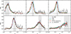 |
Fig. 10. Comparison of the ensemble of MICE2 realisations and their best-fit solutions when using the SOM redshift distributions as model for the shift-fit. The black data points indicate the mean and standard deviation (encapsulating the added intrinsic scatter) of the CC measurement realisations, the green and blue lines represent the true and SOM redshift distributions, respectively. The red line and shaded area (median and 68% confidence interval) is the NSOM(z) after applying the shift-fit parameter value in each realisation. |
6.2.2. CCs fitted with true redshift distributions
First, we needed to verify that our updated measurement process and fitting procedure were able to accurately reproduce the true redshifts of the MICE2 galaxies. Therefore, we fit the CC measurements with the true redshift distribution to check whether the resulting shift parameter  was consistent with zero in all bins. We compared a number of different correlation measurement scales and found that excluding the smallest scales (r < 0.5 Mpc) resulted in the least biased shift parameters, whereas setting the upper limit to 1.5 Mpc still maintained a good S/N in the correlation amplitude. Therefore, we chose 0.5 < r ≤ 1.5 Mpc as fiducial measurement scale for KiDS-Legacy.
The ensemble of parameter values from all realisations of this setup, fitted with the true redshift distribution, are listed in Table 7 and shown by the green data points in Fig. 11. Most importantly, all shift-fit values are consistent with zero and  (except for bin six), demonstrating that our new methodology is able to produce unbiased estimates of the underlying true redshift distribution. In the first four tomographic bins, where most of the redshift distributions are covered by the wide area spectroscopic samples of 2dFLenS, BOSS, and GAMA, the scatter in
  is 0.005. In bins five and six, which are dominated by the CCs from DESI, the scatter is significantly larger (0.017 and 0.044) with the largest shift of
 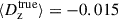 inbin six.
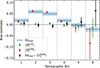 |
Fig. 11. Mean and scatter of the shift parameters obtained from the 100 MICE2 realisations with noise adaptation. The blue line and shaded area indicate the bias in the median SOM redshift, the green and red data points indicate the mean and scatter of the shift-fit parameters Dz when fitting the realisations with either the true or SOM redshift distribution. The black data points represent the difference between the empirical SOM bias estimate and the shift-fit parameter. |
Parameters and goodness of fit obtained from CC analyses.
We found that our fitting approach, with the additional error term that accounted for intrinsic scatter, was able (on average) to reproduce the input value from the measurements of the data. The scatter of the f-values between realisations was similar to the uncertainty of the input value. The distribution of goodness-of-fit values was consistent with χ2/dof = 1 in all bins, as was expected given the model’s ability to increase the magnitude of the uncertainty.
6.2.3. CCs fitted with SOM redshift distributions
The second step of verifying our pipeline was fitting the mock CCs with the SOM redshift distributions and comparing the shift parameters to the bias in the median SOM redshift (δzmed). Ideally, both values should be in agreement if the difference between the CCs and NSOM(z) can, to first order, be rectified by a simple shift in redshift.
The goodness of fit for these fits is, similar to the case of fitting with the true redshift distributions above, consistent with χdof2 = 1. The fitted f-values are up to 50 % larger compared to the previous case but are otherwise, with the exception of bin one, fully consistent with the input values from the data when considering the uncertainty and the scatter between the realisations (see Table 7). The shift-parameter values are much larger when using the NSOM(z) as fit model and only consistent with zero in bin five; see the red data points in Fig. 11. In bins one to four,  is largely positive, indicating that the SOM overestimates the median redshift by about 0.015 in bins one and four and up to 0.060 in bin two. In general, the scatter in
  is similar to the ones obtained from the fits with the true redshift distribution.
While these values indicated a large bias in the SOM redshifts, they are perfectly consistent with the SOM bias reported for this specific version of MICE2 (compare Table 6 and the blue confidence regions in Fig. 11). When we take the difference  of the two bias estimates, the value is consistent with zero considering the scatter of
  between the noise realisations, as indicated by the black data points in Fig. 11. The scatter is about 0.012 in the first four bins and 0.022 and 0.072 in bins five and six, respectively. The amplitude of the difference is less than 0.01 in all but the last two tomographic bins, of which bin six is particularly poorly constrained.
Finally, we confirmed visually in Fig. 10 that applying the shift to the NSOM(z) on MICE2 results in a much better match with the CCs than the unshifted redshifts. Especially in bins two and three, where  is large, the peak of the distribution closely matches the realisations of the CCs after shifting. There are some remaining residual differences near the tails of the distributions, which probably explain the increase in the best-fit f-values.
7. Data results
7.1. SOM redshift distributions
Figure 12 presents the redshift distributions estimated for the six tomographic bins using the SOM algorithm, for a range of different analysis choices. The results are largely indistinguishable from one-another, except that there are two sets of lines; those using the prior volume weighting and those without. As shown in Sect. 4.3, this is for two reasons. Firstly the prior volume weight acts to smooth the large-scale structure that is imprinted on the redshift distribution of the calibration sample, leading to smoother estimates of the wide-field N(z). Secondly, as shown in Fig. 6, the prior volume weights are able to introduce systematic shifts in the tomographic redshift distributions of the calibration sample before SOM re-weighting. The shifts in Fig. 12 are less significant than the example shown in Fig. 6, however, demonstrating that the SOM re-weighting has acted to undo some of the prior weight shift.
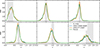 |
Fig. 12. Estimated redshift distributions from the SOM method, for different analysis choices. Results are highly consistent, except when switching between use or non-use of the prior volume weighting. However, as described in Sect. 4.3, this difference is shown to be reflected in an increased bias for the non-prior-weighted distributions. |
The resulting N(z) in Fig. 12 are each associated with an estimated bias, and it is worth noting that the difference in the redshift distributions is almost perfectly compensated by the change in bias predicted by SKiLLS. Said differently, the response of the data N(z) to the prior weight is exactly the same as the response of the simulated N(z) to the prior weight. This is a further indication that the simulated analysis used to estimate the bias parameters faithfully reproduces the complexity of thereal data.
Finally, we note the similarity between the redshift distributions estimated on the data and on the simulations. In particular bins two to five are essentially identical as estimated on SKiLLS and on the data. Bin six shows the most significant differences: the simulated redshift distribution has a considerable smoothly decreasing tail extending to redshift two, whereas the data N(z) all truncate fairly abruptly at z ≈ 1.6. We have not explored the origin of this difference here, but note that such a difference will be enhanced by slight differences in the signal-to-noise and size properties of the most distant sources. We attempted to remove such differences using our matching process; however, this difference may indicate that there is still some residual difference between the data and mock galaxies at high redshift.
7.2. CC redshift distributions
Similar to the mock analysis in Sect. 6.2.3, we measured the clustering redshifts of the KiDS-Legacy lensing sample, computed the joint, inverse-variance weighted CC estimate, and performed the shift-fitting with the fiducial SOM redshift distributions (see above). The final CC measurements are presented in Fig. 13. In general, these are (in part due to the noise adaptation) very similar to the ensemble average of the MICE2 realisations (Fig. 10).
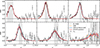 |
Fig. 13. Comparison of the fiducial data CCs, SOM redshift distributions (used as fit model, re-normalised to the fitted amplitude of the CCs, and additionally with the estimated SOM bias corrected), and shift-fit posterior median and 68% confidence interval. The additional grey error bar whiskers indicate the total confidence interval that includes the fitted intrinsic scatter. |
7.2.1. CCs fitted with SOM redshifts
As a result, the shift-fit parameters  follow as similar trend as those of MICE2 (Table 7). One major difference is that we observed some additional intrinsic scatter, especially at z > 1.0, where DESI dominates the joint CC measurements, which our simple f-term model was unable to fully capture. The best-fit f-term is a small fraction of the total uncertainty of the CC measurements10 (Fig. 13).
This difference was also reflected in the increased uncertainty of  in the last three tomographic bins, where it reached
  in bin six. Since we are limited to the maximum redshift of our DESI sample at z ≈ 1.6, the consequence is that the mean redshift of bin six was not very well constrained by the clustering redshifts. In the five other bins, the uncertainty was found to be at a similar level as MICE2. The magnitude of the shifts is in general smaller for the first three tomographic bins, reaching a maximum of 0.028 in bin two, which is clearly in agreement with visible offset between the SOM and the CCs in Fig. 13. In bins four and five, the magnitude of the shift is similar to bins two and three, but in bin six it reaches
  , preferring a shift of the NSOM(z) at low significance to higher redshifts. Overall, only bins one and five are unbiased according to the shift-fit after taking the uncertainties into account.
7.2.2. Comparison to SOM bias from SKiLLS
As a final test, we used the fitted shift-parameters  to test how well the SOM calibration of the SKiLLS simulation represented the SOM calibration of the KiDS-Legacy data. Similar to our analysis of the MICE2 data (Sect. 6.2.3) we compared
  to the bias of the median SOM redshifts obtained from SKiLLS (see Table 8 and Fig. 14) and found that they are not identical, but closely follow the same trends. The bias is consistent with zero in bin one, positive for bins two to four, and smoothly transitions to negative values in bins five and six. In general, the biases indicated by the
  are somewhat larger than the SOM biases in SKiLLS. However, when factoring in the uncertainties, the difference
  is consistent with zero in all bins, except for bin four, which exhibits an approximately 2σ difference, again driven by the CCs preferring larger measured biases.
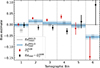 |
Fig. 14. Comparison of the shift parameters obtained from the KiDS-Legacy data and the SOM bias obtained from SKiLLS. The short grey and blue lines indicate the bias in the mean and median SOM redshift, the red data points the shift-fit parameters Dz when fitting CC measurements with the NSOM(z). The black data points represent the difference between the empirical median SOM bias estimate and the shift-fit parameter. |
Different redshift bias estimates per tomographic bin obtained from the KiDS-Legacy data.
This comparison also highlights that  is most closely comparable to the median SOM bias instead of the mean. In particular, the mean redshift of bin one is very sensitive to small fractions of high-redshift, catastrophic outlier populations, to which the measured CCs and the core of the NSOM(z), and in turn
  , are insensitive.
8. Discussion
The results presented in the previous sections form the basis for measurements of WL with the KiDS-Legacy dataset. Using extensive mock catalogues, we quantified the precision and accuracy of the redshift calibration of the six tomographic bins used in those measurements. In the following, we highlight the most important aspects and lessons learned from this calibration effort.
We relied heavily on mock catalogues that resemble the KiDS and KiDZ data in many important aspects (colour-redshift relation, photometric noise level, photo-z quality, clustering properties, etc.). This reliance makes it necessary to introduce redundancy in the underlying simulations to test the robustness of the results to the assumptions in the creation of the simulations. The two simulations used in this work are quite different. SKiLLS is based on a semi-analytic galaxy model, a full simulation of KiDS/VIKING images, and a replication of the KiDS photometry and shape-measurement pipelines on these synthetic images. It also extends to high redshifts (z < 2.3) covering the whole redshift range of interest for KiDS. Our MICE2 mocks are more simplistic as we do not implement a full image simulation here, employ a parametric model for photometric noise, and add shape-measurement weights in a rather ad hoc way. Also, MICE2 is limited to z < 1.4, which compromises its ability to calibrate the highest redshifts probed by KiDS. However, it covers a much larger area than SKiLLS, which makes it useful for clustering redshift analyses.
Most importantly, the two simulations are inherently so different that any agreement of the calibration results between SKiLLS (truncated at z < 1.4 for comparison) and MICE2 can be regarded as a strong sign of systematic robustness. This is exactly what we observe with the SOM calibration for the calibration samples that are most comparable between the two simulations, meaning the samples without lensfit weights (as those weights are not entirely realistic in MICE2); see the Δ⟨δz⟩ rows of scenarios [J] (vs [H]) and [K] (vs [I]) in Table 5. While the actual calibration sample used in the cosmological analysis looks slightly different (i.e. using shape weights) and the redshift bias values themselves will be different (e.g. compare ⟨δz⟩ of scenarios [A] and [E]), there is no reason to assume that the robustness is affected by these differences. Hence, we use the reported Δ⟨δz⟩ to motivate a conservative systematic error floor of δz = 0.01 for our SOM results. Hence, the SKiLLS SOM results, verified with the MICE2 SOM runs, yield a primary, simulation-based validation of the SOM N(z) on the KiDS data at the per cent level in terms of the mean redshift, which is exactly what is required for the full, uncompromised cosmological exploitation of cosmic shear with KiDS-Legacy.
The CC methodology with the KiDS-Legacy calibration samples is tested extensively on MICE2 and shown to be unbiased within errors if the true N(z) are used as a model in the shift fit. The goodness of fit is satisfactory when we inflate the errors of the CC measurements and the noise according to what we observe on the data. The necessity for this adaptation highlights a possible shortcoming of the MICE2 simulations that do not seem to replicate the full complexity of systematic effects in the data. Still, with this adaptation, the similarity between the CC measurements on the data and simulations gives us confidence in the applicability of the MICE2 results.
Most importantly for our efforts, the CC method is able to correct the bias inherent to the SOM N(z) on MICE2 when those are used as a model in the shift fit. This non-trivial result reported in Fig. 11 and Table 6 establishes the CC as a secondary, data-based method for N(z) validation.
The crucial question is then whether the highly complementary primary and secondary validation methods agree on the data. This is answered positively by Fig. 14. The residual bias of the KiDS SOM N(z) suggested by SKiLLS agrees with the bias suggested by shift-fitting the KiDS SOM N(z) to the KiDS CC measurements. The only exception is bin four, which exhibits a 2σ shift towards negative values; however, such a single shift will not have a significant impact on the cosmological results. The two methods of validation mentioned are similarly precise in the first three tomographic bins. In bins five and six, the clustering redshifts still suffer from limited calibration samples and possibly further systematics that affect the increasingly faint target samples, for example, spurious density variations due to variable depth and seeing.
The residual biases and their uncertainties can be directly translated into priors on the mean redshifts used in the cosmological inference of KiDS cosmic shear measurements. The discussion above motivates at least two main scenarios, one that relies fully on the SOM N(z) and their calibration with SKiLLS and a second one using the SOM N(z) but calibrated with the CC measurements instead. It is clear that in the latter case the very loose priors on the mean redshifts of bins five and six would severely compromise the constraining power of these bins. So this CC-calibrated setup would constitute a very conservative approach. Even the tighter, SKiLLS-calibrated priors should still be regarded as conservative because the error floor introduced due to residual differences between the SOM runs on SKiLLS (truncated) and MICE2 is erring on the side of caution. There are very good reasons to believe in the superiority of the SKiLLS results. If we took those at face value, we would end up with priors on the mean redshifts that approach the level of completed stage-IV cosmic shear surveys (see row σδz of scenario [A] of Table 5).
9. Summary
In this paper we have presented the redshift calibration of the final KiDS WL dataset, dubbed KiDS-Legacy and based on KiDS-DR5. We developed a calibration strategy that involves multiple levels of redundancy to ensure that we met the requirement of an accuracy of the mean redshifts of the tomographic bins used for cosmic shear at the percent level.
The first level of redundancy is represented by the use of two complementary sets of mock catalogues extracted from two quite different types of simulations, SKiLLS and MICE2. Using a newly developed matching algorithm, we arrive at mock catalogues that are highly realistic and emulate the data (i.e. the KiDS WL sources as well as spectroscopic calibration samples) with high fidelity.
The second level of redundancy is represented by two different calibration techniques, a colour-based SOM calibration and a position based clustering redshift technique. This combination has become the standard in contemporary WL analyses and is further strengthened here by an extensive overlap of KiDS-DR5 with different spectroscopic surveys and an almost complete disconnect of the spectroscopic calibration samples used for either technique.
We show, in essence, that running the SOM on one simulation can be used to calibrate the WL sources in the other simulation with residual bias ⟨δz⟩≲0.01. Given that we estimate the match between the more sophisticated simulation, SKiLLS, and the KiDS data to be at least as good as the match between SKiLLS and MICE2, we are confident that SKiLLS can calibrate the SOM N(z) of KiDS at the same level of accuracy or better. The great similarity between the N(z) of the simulated SKiLLS sources and the N(z) estimated with the SOM on the data further justifies the applicability of this conclusion to the KiDS dataset.
Additionally, we show that the clustering redshifts are able to correct for any residual bias in the SOM N(z) on the MICE2 simulation. With this result in mind, we ran the clustering redshift technique on the data, shift-fitting the SOM N(z) to the clustering measurements and found biases that agree with the purely simulated bias estimates from SKiLLS. This again mirrors the results of MICE2 clustering-z vs SKiLLS SOM N(z), which further validates the realism of the simulations. Passing this strong consistency test suggests a robust calibration and a successful understanding and correction of systematic errors at the percent level in terms of the mean redshifts of the tomographic bins.
These results have been used to define the priors on the mean redshifts of the tomographic bins in the cosmic shear analyses of KiDS-Legacy (Wright et al. 2025; Stölzner et al. 2025). A SKiLLS-based SOM N(z) calibration with a conservative error floor constitutes the fiducial setup, taking the form of informative correlated Gaussian priors with means δz = { − 2.6, 1.4, −0.2, 0.8, −1.1, −5.4}×10−2 and standard deviation σδz ≈ 0.01. As an alternative, we also present a purely empirical, somewhat less constraining setup that takes the clustering redshift results as (differently correlated) priors that make the cosmological conclusions independent of simulations of the redshift calibration.
With the type of data used here, we reach statistical uncertainties on the mean redshifts with our SOM implementation of σ(⟨δz⟩) ≈ 0.002, which falls within the range of the requirement for Euclid. This suggests that, in terms of methodology and calibration data, we are almost ready to calibrate a stage-IV cosmic shear survey. Certainly, the redshift range has to be extended to z ∼ 2, but this is well within reach. The real challenge will be to reduce the systematic error floor, conservatively estimated here, by about a factor of 5. This will require a set of a few highly realistic, complementary simulations that capture the whole complexity of a future cosmic shear experiment.
The statistical uncertainties on the clustering redshifts shown here are still at least a factor of 3 greater than those required by Euclid. With an order of magnitude more area in the WL samples and the full power of upcoming wide-field spectroscopic calibration samples (a glimpse is given here with just ∼105 DESI EDR galaxies), this factor of 3 is within reach. Systematic error control will be paramount here as well, and will be similarly achieved through redundancy in the simulations that validate the calibration.
Visible and Infrared Survey Telescope for Astronomy.
We emphasise here the importance of the inequalities used in these definitions: as the photo-z estimates are discrete with finite steps of 0.01, whether one uses zB ≤ 0.9 or zB < 0.9 has a non-negligible impact on the sample definition.
For our fiducial N(z) binning, Δz = 0.05, the primary probability mass of each N(z) is sampled by ten or more bins. This means that the difference introduced when computing the sample mean redshift vs N(z) expectation is negligible.
While counting pairs only within the same region can have an effect on the overall correlation amplitude, it has no effect on any of our previously published results because this overall amplitude is later normalised.
These scales are larger than what was used in previous KiDS clustering redshift analyses. See Sect. 6.2.2 for a justification.
The normalisation is necessary because we cannot expect the data points to be properly normalised a priori due to galaxy bias or other systematic effects.
When including smaller measurement scales, the f-term contribution becomes significant.
Acknowledgments
AHW and HHi are supported by the Deutsches Zentrum für Luft- und Raumfahrt (DLR), made possible by the Bundesministerium für Wirtschaft und Klimaschutz, under project 50QE2305, and acknowledge funding from the German Science Foundation DFG, via the Collaborative Research Center SFB1491 “Cosmic Interacting Matters - From Source to Signal”. HHi is also supported by a DFG Heisenberg grant (Hi 1495/5-1). HHi, JLvdB, CM, RR, & AD are supported by an ERC Consolidator Grant (No. 770935). MB & PJ are supported by the Polish National Science Center through grant no. 2020/38/E/ST9/00395. MB is also supported by grant no. 2020/39/B/ST9/03494. CH, BS, & ZY acknowledge support from the Max Planck Society and the Alexander von Humboldt Foundation in the framework of the Max Planck-Humboldt Research Award endowed by the Federal Ministry of Education and Research. CH also acknowledges support from the UK Science and Technology Facilities Council (STFC) under grant ST/V000594/1. BJ acknowledges support by the ERC-selected UKRI Frontier Research Grant EP/Y03015X/1 and by STFC Consolidated Grant ST/V000780/1. CM acknowledges support from the Beecroft Trust, and the Spanish Ministry of Science under the grant number PID2021-128338NB-I00. MA is supported by the UK Science and Technology Facilities Council (STFC) under grant number ST/Y002652/1 and the Royal Society under grant numbers RGSR2222268 and ICAR1231094. CG is funded by the MICINN project PID2022-141079NB-C32. BG acknowledges support from the UKRI Stephen Hawking Fellowship (grant reference EP/Y017137/1). HHo & MY acknowledge support from the European Research Council (ERC) under the European Union’s Horizon 2020 research and innovation program with Grant agreement No. 101053992. SJ acknowledges the Ramón y Cajal Fellowship (RYC2022-036431-I) from the Spanish Ministry of Science and the Dennis Sciama Fellowship at the University of Portsmouth. KK acknowledges support from the Royal Society and Imperial College. SSL is receiving funding from the programme “Netzwerke 2021”, an initiative of the Ministry of Culture and Science of the State of North-Rhine Westphalia. LL is supported by the Austrian Science Fund (FWF) [ESP 357-N]. AL acknowledges support from the research project grant ‘Understanding the Dynamic Universe’ funded by the Knut and Alice Wallenberg Foundation under Dnr KAW 2018.0067. LM acknowledges the financial contribution from the grant PRIN-MUR 2022 20227RNLY3 “The concordance cosmological model: stress-tests with galaxy clusters" supported by Next Generation EU and from the grant ASI n. 2024-10-HH.0 ‘Attivitá scientifiche per la missione Euclid – fase E’. LP acknowledges support from the DLR grant 50QE2002. MR acknowledges financial support from the INAF grant 2022. TT acknowledges funding from the Swiss National Science Foundation under the Ambizione project PZ00P2_193352. MvWK acknowledges the support by the UKSA and STFC (grant no. ST/X001075/1). YZ acknowledges the studentship from the UK Science and Technology Facilities Council (STFC). Based on observations made with ESO Telescopes at the La Silla Paranal Observatory under programme IDs 179.A-2004, 177.A-3016, 177.A-3017, 177.A-3018, 298.A-5015. Author Contributions: All authors contributed to the development and writing of this paper. The authorship list is given in three groups: the lead authors (AHW, HHi, JLvdB), followed by two alphabetical groups. The first alphabetical group includes those who are key contributors to both the scientific analysis and the data products of this manuscript and release. The second group covers those who have made a significant contribution either to the preparation of data products or to the scientific analyses of KiDS-Legacy.
References
- Aihara, H., AlSayyad, Y., Ando, M., et al. 2022, PASJ, 74, 247 [NASA ADS] [CrossRef] [Google Scholar]
- Alam, S., Albareti, F. D., Allende Prieto, C., et al. 2015, ApJS, 219, 12 [Google Scholar]
- Anderson, T. W., & Darling, D. A. 1954, J. Am. Stat. Assoc., 49, 765 [Google Scholar]
- Begeman, K., Belikov, A. N., Boxhoorn, D. R., & Valentijn, E. A. 2013, Exp. Astron., 35, 1 [NASA ADS] [Google Scholar]
- Benítez, N. 2000, ApJ, 536, 571 [Google Scholar]
- Bertin, E., & Arnouts, S. 1996, A&AS, 117, 393 [NASA ADS] [CrossRef] [EDP Sciences] [Google Scholar]
- Bianchi, D., Burden, A., Percival, W. J., et al. 2018, MNRAS, 481, 2338 [Google Scholar]
- Blake, C., Amon, A., Childress, M., et al. 2016, MNRAS, 462, 4240 [NASA ADS] [CrossRef] [Google Scholar]
- Carretero, J., Castander, F. J., Gaztañaga, E., Crocce, M., & Fosalba, P. 2015, MNRAS, 447, 646 [NASA ADS] [CrossRef] [Google Scholar]
- Coil, A. L., Mendez, A. J., Eisenstein, D. J., & Moustakas, J. 2017, ApJ, 838, 87 [Google Scholar]
- Crocce, M., Castander, F. J., Gaztañaga, E., Fosalba, P., & Carretero, J. 2015, MNRAS, 453, 1513 [NASA ADS] [CrossRef] [Google Scholar]
- Davis, M., & Peebles, P. J. E. 1983, ApJ, 267, 465 [Google Scholar]
- DESI Collaboration (Aghamousa, A., et al.) 2016a, arXiv e-prints [arXiv:1611.00036] [Google Scholar]
- DESI Collaboration (Aghamousa, A., et al.) 2016b, arXiv e-prints [arXiv:1611.00037] [Google Scholar]
- DESI Collaboration (Adame, A. G., et al.) 2024, AJ, 168, 58 [NASA ADS] [CrossRef] [Google Scholar]
- Driver, S. P., Bellstedt, S., Robotham, A. S. G., et al. 2022, MNRAS, 513, 439 [NASA ADS] [CrossRef] [Google Scholar]
- Edge, A., Sutherland, W., Kuijken, K., et al. 2013, The Messenger, 154, 32 [NASA ADS] [Google Scholar]
- Elahi, P. J., Welker, C., Power, C., et al. 2018, MNRAS, 475, 5338 [NASA ADS] [CrossRef] [Google Scholar]
- Euclid Collaboration (Mellier, Y., et al.) 2025, A&A, 697, A1 [Google Scholar]
- Fenech Conti, I., Herbonnet, R., Hoekstra, H., et al. 2017, MNRAS, 467, 1627 [NASA ADS] [Google Scholar]
- Fosalba, P., Crocce, M., Gaztañaga, E., & Castander, F. J. 2015a, MNRAS, 448, 2987 [NASA ADS] [CrossRef] [Google Scholar]
- Fosalba, P., Gaztañaga, E., Castander, F. J., & Crocce, M. 2015b, MNRAS, 447, 1319 [NASA ADS] [CrossRef] [Google Scholar]
- Garilli, B., Guzzo, L., Scodeggio, M., et al. 2014, A&A, 562, A23 [NASA ADS] [CrossRef] [EDP Sciences] [Google Scholar]
- Gatti, M., Giannini, G., Bernstein, G. M., et al. 2022, MNRAS, 510, 1223 [Google Scholar]
- Gruen, D., & Brimioulle, F. 2017, MNRAS, 468, 769 [Google Scholar]
- Hartley, W. G., Chang, C., Samani, S., et al. 2020, MNRAS, 496, 4769 [Google Scholar]
- Heydenreich, S., Schneider, P., Hildebrandt, H., et al. 2020, A&A, 634, A104 [NASA ADS] [CrossRef] [EDP Sciences] [Google Scholar]
- Hildebrandt, H., Arnouts, S., Capak, P., et al. 2010, A&A, 523, A31 [NASA ADS] [CrossRef] [EDP Sciences] [Google Scholar]
- Hildebrandt, H., Viola, M., Heymans, C., et al. 2017, MNRAS, 465, 1454 [Google Scholar]
- Hildebrandt, H., Köhlinger, F., van den Busch, J. L., et al. 2020, A&A, 633, A69 [NASA ADS] [CrossRef] [EDP Sciences] [Google Scholar]
- Hildebrandt, H., van den Busch, J. L., Wright, A. H., et al. 2021, A&A, 647, A124 [EDP Sciences] [Google Scholar]
- Huterer, D., Takada, M., Bernstein, G., & Jain, B. 2006, MNRAS, 366, 101 [Google Scholar]
- Ivezić, Ž., Kahn, S. M., Tyson, J. A., et al. 2019, ApJ, 873, 111 [Google Scholar]
- Joachimi, B., Lin, C. A., Asgari, M., et al. 2021, A&A, 646, A129 [NASA ADS] [CrossRef] [EDP Sciences] [Google Scholar]
- Johnson, A., Blake, C., Amon, A., et al. 2017, MNRAS, 465, 4118 [Google Scholar]
- Kuijken, K. 2008, A&A, 482, 1053 [NASA ADS] [CrossRef] [EDP Sciences] [Google Scholar]
- Kuijken, K., Heymans, C., Dvornik, A., et al. 2019, A&A, 625, A2 [NASA ADS] [CrossRef] [EDP Sciences] [Google Scholar]
- Lagos, C. d. P., Tobar, R. J., Robotham, A. S. G., et al. 2018, MNRAS, 481, 3573 [CrossRef] [Google Scholar]
- Landy, S. D., & Szalay, A. S. 1993, ApJ, 412, 64 [Google Scholar]
- Li, S.-S., Kuijken, K., Hoekstra, H., et al. 2023, A&A, 670, A100 [NASA ADS] [CrossRef] [EDP Sciences] [Google Scholar]
- Lima, M., Cunha, C. E., Oyaizu, H., et al. 2008, MNRAS, 390, 118 [Google Scholar]
- Linke, L., Unruh, S., Wittje, A., et al. 2025, A&A, 693, A210 [NASA ADS] [CrossRef] [EDP Sciences] [Google Scholar]
- MacCrann, N., Becker, M. R., McCullough, J., et al. 2022, MNRAS, 509, 3371 [Google Scholar]
- McFarland, J. P., Verdoes-Kleijn, G., Sikkema, G., et al. 2013, Exp. Astron., 35, 45 [Google Scholar]
- McLeod, M., Balan, S. T., & Abdalla, F. B. 2017, MNRAS, 466, 3558 [NASA ADS] [CrossRef] [Google Scholar]
- Miller, L., Kitching, T. D., Heymans, C., Heavens, A. F., & van Waerbeke, L. 2007, MNRAS, 382, 315 [Google Scholar]
- Miller, L., Heymans, C., Kitching, T. D., et al. 2013, MNRAS, 429, 2858 [Google Scholar]
- Morrison, C. B., Hildebrandt, H., Schmidt, S. J., et al. 2017, MNRAS, 467, 3576 [Google Scholar]
- Myles, J., Alarcon, A., Amon, A., et al. 2021, MNRAS, 505, 4249 [NASA ADS] [CrossRef] [Google Scholar]
- Naidoo, K., Johnston, H., Joachimi, B., et al. 2023, A&A, 670, A149 [NASA ADS] [CrossRef] [EDP Sciences] [Google Scholar]
- Newman, J. A. 2008, ApJ, 684, 88 [Google Scholar]
- Newman, J. A., & Gruen, D. 2022, ARA&A, 60, 363 [NASA ADS] [CrossRef] [Google Scholar]
- Newman, J. A., Abate, A., Abdalla, F. B., et al. 2015, Astropart. Phys., 63, 81 [Google Scholar]
- Rau, M. M., Dalal, R., Zhang, T., et al. 2023, MNRAS, 524, 5109 [NASA ADS] [CrossRef] [Google Scholar]
- Reischke, R. 2024, MNRAS, 530, 4412 [NASA ADS] [CrossRef] [Google Scholar]
- Reischke, R., Unruh, S., Asgari, M., et al. 2025, A&A, 699, A124 [NASA ADS] [CrossRef] [EDP Sciences] [Google Scholar]
- Schmidt, S. J., Ménard, B., Scranton, R., Morrison, C., & McBride, C. K. 2013, MNRAS, 431, 3307 [Google Scholar]
- Scodeggio, M., Guzzo, L., Garilli, B., et al. 2018, A&A, 609, A84 [NASA ADS] [CrossRef] [EDP Sciences] [Google Scholar]
- Sevilla-Noarbe, I., Bechtol, K., Carrasco Kind, M., et al. 2021, ApJS, 254, 24 [NASA ADS] [CrossRef] [Google Scholar]
- Sipp, M., Schäfer, B. M., & Reischke, R. 2021, MNRAS, 501, 683 [Google Scholar]
- Stölzner, B., Joachimi, B., Korn, A., Hildebrandt, H., & Wright, A. H. 2021, A&A, 650, A148 [NASA ADS] [CrossRef] [EDP Sciences] [Google Scholar]
- Stölzner, B., Wright, A. H., Asgari, M., et al. 2025, A&A, 702, A169 [NASA ADS] [CrossRef] [EDP Sciences] [Google Scholar]
- Valentijn, E. A., McFarland, J. P., Snigula, J., et al. 2007, in Astronomical Data Analysis Software and Systems XVI, eds. R. A. Shaw, F. Hill, & D. J. Bell, ASP Conf. Ser., 376, 491 [Google Scholar]
- van den Busch, J. L., Hildebrandt, H., Wright, A. H., et al. 2020, A&A, 642, A200 [NASA ADS] [CrossRef] [EDP Sciences] [Google Scholar]
- van den Busch, J. L., Wright, A. H., Hildebrandt, H., et al. 2022, A&A, 664, A170 [NASA ADS] [CrossRef] [EDP Sciences] [Google Scholar]
- Wright, A. H., Hildebrandt, H., Kuijken, K., et al. 2019, A&A, 632, A34 [NASA ADS] [CrossRef] [EDP Sciences] [Google Scholar]
- Wright, A. H., Hildebrandt, H., van den Busch, J. L., & Heymans, C. 2020a, A&A, 637, A100 [NASA ADS] [CrossRef] [EDP Sciences] [Google Scholar]
- Wright, A. H., Hildebrandt, H., van den Busch, J. L., et al. 2020b, A&A, 640, L14 [NASA ADS] [CrossRef] [EDP Sciences] [Google Scholar]
- Wright, A. H., Kuijken, K., Hildebrandt, H., et al. 2024, A&A, 686, A170 [NASA ADS] [CrossRef] [EDP Sciences] [Google Scholar]
- Wright, A. H., Stölzner, B., Asgari, M., et al. 2025, A&A, in press https://doi.org/10.1051/0004-6361/202554908 [Google Scholar]
- Yan, Z., Wright, A. H., Elisa Chisari, N., et al. 2025, A&A, 694, A259 [NASA ADS] [CrossRef] [EDP Sciences] [Google Scholar]
Appendix A: Sample selection function for MICE2
In our clustering redshift analysis with simulated data based on MICE2 we aimed to replicate the observational datasets as closely as possible. Since we added spectroscopic data from the DESI EDR and VIPERS PDR-2, we also needed to implement their selection functions for MICE2, similar to the procedure already adopted in van den Busch et al. (2020). Where possible, we applied the same selection criteria used for the spectroscopic target selection and used sampling strategies to implement additional selection effects, such as spectroscopic success rates, and to mitigate systematic differences between MICE2 and the observed datasets.
A.1. DESI EDR data
We used a subset (called the LSS catalogues) of the DESI LRG and ELG samples for the KiDS-Legacy clustering redshifts. The target selection for the ELG sample is a simple colour-magnitude cut, which can, in principle, be applied directly to MICE2. The LRG sample, however, and some of the additional selections applied for the construction of the LSS catalogues, depend on observed quantities to which we do not have access to in MICE2. Therefore, we decided to implement the DESI selection function for MICE2 by mostly relying on sampling techniques.
We selected the LRG and ELG sample jointly by performing a number of selection steps. First, we split the DESI data and MICE2 into bins of redshift (Δz = 0.05). In each of these bins we computed the expected number of ELGs, LRGs, and (although not utilised) quasars (QSOs). Then we randomly draw the appropriate number QSOs from MICE2 by requiring 19.5 < r < 23.4 without any further selections (MICE2 does not contain any QSOs specifically) and discarded them. From the remaining MICE2 galaxies we then selected the expected number of ELGs by picking the objects with the highest specific star formation rate that fell in the magnitude window 20.0 < g < 24.1. Finally, we drew the expected number of LRGs from those MICE2 galaxies that were not already assigned to either the QSO or ELG sample. We selected objects with the highest stellar mass, and at magnitude z < 21.61. This procedure ensures that the MICE2 DESI sample has the correct redshift distribution by design. Figure A.1 shows the distribution of stellar mass and star-formation rate of galaxies in all of MICE2 and those in our simulated DESI subset. The LRG and ELG subsets are clearly separated in stellar mass, the ELG sample contains mostly objects with low stellar mass but high star-formation rate.
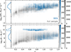 |
Fig. A.1. Comparison of the star-formation rate (top) and the stellar mass (bottom) for the full MICE simulation (grey) and our simulated DESI LRG and ELG samples (blue) as a function of redshift. The data is selected from a 44 deg2 patch of MICE2. The lower panel clearly shows the separation of the ELG from the LRG sample, which is selected based on stellar mass. |
To verify our new selection function we compared its clustering amplitude wss with the one we obtain from DESI. We measured the angular correlation between 100 and 1000 kpc and found good agreement between simulation and data for most redshifts, except around the redshifts 0.85 and 1 (see Fig. A.2). Since we were already selecting objects with low stellar mass in our ELG selection (for which we already expect a lower galaxy bias and therefore a lower clustering amplitude; see e.g. Coil et al. 2017), we speculate that this may be an inherent property of MICE2.
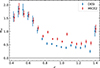 |
Fig. A.2. Auto-correlation amplitude measured between 100 and 1000 kpc for DESI (in blue) and MICE2 (in red). |
A.2. VIPERS data
VIPERS targets galaxies with magnitude iAB ≤ 22.5 and an additional colour selection that aims to isolate galaxies at z > 0.5 (Scodeggio et al. 2018):
 (A.1)
(A.1)
We applied the same selection criteria to MICE2.
This colour selection (colour sampling rate) leads to a completeness that transitions from almost zero to one in the range of 0.4 < z < 0.6. There are two additional effects that need to be factored in to obtain the total completeness of the sample; the target sampling rate (TSR), which is about 50 % on average but has a strong positional dependence due to observational and instrumental limitations, and the spectroscopic success rate (SSR). The total completeness is a product of these three terms and VIPERS defines a weight to account for this incompleteness as
 (A.2)
(A.2)
For our purposes, we chose to not model the positional dependence of the TSR and simply estimate the mean incompleteness weight empirically in the redshift range 0.6 ≤ z < 1.18 (see Sect. 2.1), as shown in Fig. A.3. When applied to MICE2 together with the VIPERS colour selection, we found that this approach reproduced the redshift distribution p(z) of the VIPERS dataset very well. However, we needed to apply an additional sparse sampling by 30 % to match the absolute number density found in the data. Similar discrepancies have been reported by van den Busch et al. (2020) when trying to reproduce the selection functions of other high redshift datasets and are most likely explained by systematic differences between MICE2 and the observational data.
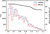 |
Fig. A.3. Comparison of the VIPERS redshifts distribution (in blue) in the range 0.6 ≤ z < 1.18 and MICE2 (in red) after applying the colour and magnitude cuts, and the empirical incompleteness sampling, indicated by the total success rate (black line). |
Similar to DESI, we verified our new selection function by comparing its clustering amplitude wss with the one we obtained from VIPERS. We measured on the same scales from 100 and 1000 kpc and found a good agreement between simulation and data, both in the amplitude as well as its uncertainty over the full redshift baseline (Fig. A.4).
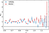 |
Fig. A.4. Auto-correlation amplitude measured between 100 and 1000 kpc for VIPERS (in blue) and MICE2 (in red). |
All Tables
Properties of the six KiDS-Legacy tomographic bins and the full source sample, using our fiducial redshift calibration procedure.
Different redshift bias estimates per tomographic bin obtained from the ensemble of MICE2 CC realisations.
Different redshift bias estimates per tomographic bin obtained from the KiDS-Legacy data.
All Figures
|
Fig. 1. Redshift distribution of the calibration data used for KiDS-Legacy. The top panel displays the full KiDZ data in grey and the proportion of it that enters each tomographic bin after calibrating the fiducial SOM, shown as a stacked histogram. The bin edges are indicated by the vertical dashed lines. The bottom panel shows the spectroscopic surveys used as calibration samples for the clustering redshift measurements (also stacked). |
| In the text | |
|
Fig. 2. Footprint of the spectroscopic surveys overlapping KiDS used for the clustering redshift measurements. VIPERS is exclusive to the KiDZ fields, which are not shown here. |
| In the text | |
|
Fig. 3. Comparison between gold-class and gold-weight definitions. Here, a SOM trained on tomographic bin one in our SKiLLS simulation is coloured by the true mean redshift of each cell (left), the gold-class definition of each cell under a single realisation (centre), and the gold weight of each cell after ten realisations. In the gold-weight panel, the cells, which are assigned a (highly stochastic) zero gold class in our single realisation, are highlighted with an orange border. These cells are assigned a wide range of final gold-weights, highlighting the stochasticity of the gold-class definition and the superiority of the gold-weights. In each colour bar, the PDF of cell values is shown. |
| In the text | |
|
Fig. 4. Distributions of gold weight per tomographic bin for our fiducial SKiLLS simulations. Individual lines show the scatter in the gold-weight PDFs under different realisations of our spectroscopic calibration samples. The tomographic bins show qualitatively similar behaviour: many sources are consistently classed as gold under all realisations of the SOM (wgold = 1), and very few sources are consistently classed as not-gold under all realisations (wgold = 0). |
| In the text | |
|
Fig. 5. Model parameters and the resulting analytic N(z) for samples defined as magnitude-limited (in the r band) from our noiseless SURFS+Shark light cone. The left and centre panels show the free parameters from Eq. (2), as a function of the r-band magnitude limit, including polynomial fits. The right panel shows the analytically estimated N(z) for each of the models parameters in the other two panels. |
| In the text | |
|
Fig. 6. Impact of prior-volume weights on the (pre-SOM) N(z) of the full spectroscopic compilation (upper panel), and on those galaxies in the compilation that end up in tomographic bin three both prior to the SOM re-weighting (middle panel) and after the SOM re-weighting (bottom panel). The systematic effect that the prior weight imparts on the tomographic bin is particularly clear prior to re-weighting by the SOM to match the wide-field sample but is somewhat diluted by the SOM re-weighting process. Nonetheless, there is a residual difference after the SOM re-weighting in the bottom panel. This difference is exacerbated if one does not have high quality image simulations to calibrate the underlying N(z) bias (dashed lines in the bottom figure; discussed further in Sect. 6), as the non-prior weighted N(z) estimate contains a significant systematic bias (⟨δz⟩≈0.03), whereas the prior weighted N(z) estimate has no bias (⟨δz⟩≈0.004). |
| In the text | |
|
Fig. 7. Example of the inverse-variance weighted combination of CCs computed from the fourth tomographic bin of MICE2. The top panel shows the individual measurements from each calibration sample, the middle panel the weighted average, and the bottom panel the relative weight of each sample as a function of redshift. |
| In the text | |
|
Fig. 8. One realisation of the CC measurements from MICE2 in the sixth tomographic bin after noise adaptation (Sect. 5.3) and the addition of intrinsic scatter (Sect 5.4). The top panel compares only the uncertainties of NCC(z) from the data (grey) and MICE2 before (blue) and after adaptation (red). The dashed black line indicates the fitted intrinsic scatter from the measurements on the data (f = 0.14 ± 0.04; see Eq. 6). The bottom panel shows the measured NCC(z) from MICE2 (blue points) compared to the data (grey line). The red data points represent the MICE2 measurements after adapting the noise (up-scaling errors and perturbing values) and adding the intrinsic scatter (only perturbing valu-es) obtained from the data. |
| In the text | |
|
Fig. 9. Redshift distributions for the fiducial SOM calibration methodology, computed using the SKiLLS simulations. The ensemble of blue polygons show the N(z) constructed with different realisations of the calibration sample. Redshift distributions include the new gold-weighting for the wide-field sample, and prior volume weighting and shape-measurement weights for the calibration samples. |
| In the text | |
|
Fig. 10. Comparison of the ensemble of MICE2 realisations and their best-fit solutions when using the SOM redshift distributions as model for the shift-fit. The black data points indicate the mean and standard deviation (encapsulating the added intrinsic scatter) of the CC measurement realisations, the green and blue lines represent the true and SOM redshift distributions, respectively. The red line and shaded area (median and 68% confidence interval) is the NSOM(z) after applying the shift-fit parameter value in each realisation. |
| In the text | |
|
Fig. 11. Mean and scatter of the shift parameters obtained from the 100 MICE2 realisations with noise adaptation. The blue line and shaded area indicate the bias in the median SOM redshift, the green and red data points indicate the mean and scatter of the shift-fit parameters Dz when fitting the realisations with either the true or SOM redshift distribution. The black data points represent the difference between the empirical SOM bias estimate and the shift-fit parameter. |
| In the text | |
|
Fig. 12. Estimated redshift distributions from the SOM method, for different analysis choices. Results are highly consistent, except when switching between use or non-use of the prior volume weighting. However, as described in Sect. 4.3, this difference is shown to be reflected in an increased bias for the non-prior-weighted distributions. |
| In the text | |
|
Fig. 13. Comparison of the fiducial data CCs, SOM redshift distributions (used as fit model, re-normalised to the fitted amplitude of the CCs, and additionally with the estimated SOM bias corrected), and shift-fit posterior median and 68% confidence interval. The additional grey error bar whiskers indicate the total confidence interval that includes the fitted intrinsic scatter. |
| In the text | |
|
Fig. 14. Comparison of the shift parameters obtained from the KiDS-Legacy data and the SOM bias obtained from SKiLLS. The short grey and blue lines indicate the bias in the mean and median SOM redshift, the red data points the shift-fit parameters Dz when fitting CC measurements with the NSOM(z). The black data points represent the difference between the empirical median SOM bias estimate and the shift-fit parameter. |
| In the text | |
|
Fig. A.1. Comparison of the star-formation rate (top) and the stellar mass (bottom) for the full MICE simulation (grey) and our simulated DESI LRG and ELG samples (blue) as a function of redshift. The data is selected from a 44 deg2 patch of MICE2. The lower panel clearly shows the separation of the ELG from the LRG sample, which is selected based on stellar mass. |
| In the text | |
|
Fig. A.2. Auto-correlation amplitude measured between 100 and 1000 kpc for DESI (in blue) and MICE2 (in red). |
| In the text | |
|
Fig. A.3. Comparison of the VIPERS redshifts distribution (in blue) in the range 0.6 ≤ z < 1.18 and MICE2 (in red) after applying the colour and magnitude cuts, and the empirical incompleteness sampling, indicated by the total success rate (black line). |
| In the text | |
|
Fig. A.4. Auto-correlation amplitude measured between 100 and 1000 kpc for VIPERS (in blue) and MICE2 (in red). |
| In the text | |
Current usage metrics show cumulative count of Article Views (full-text article views including HTML views, PDF and ePub downloads, according to the available data) and Abstracts Views on Vision4Press platform.
Data correspond to usage on the plateform after 2015. The current usage metrics is available 48-96 hours after online publication and is updated daily on week days.
Initial download of the metrics may take a while.