| Issue |
A&A
Volume 703, November 2025
|
|
|---|---|---|
| Article Number | A168 | |
| Number of page(s) | 20 | |
| Section | Stellar structure and evolution | |
| DOI | https://doi.org/10.1051/0004-6361/202555030 | |
| Published online | 20 November 2025 | |
Optical and near-infrared observations of SN 2023ixf for over 600 days after the explosion
1
Department of Physics, Tsinghua University, Beijing 100084, China
2
Department of Astronomy, University of California, Berkeley, CA 94720-3411, USA
3
INAF – Osservatorio Astronomico di Padova, Vicolo dell’Osservatorio 5, 35122 Padova, Italy
4
INAF – Osservatorio Astronomico di Brera, Via E. Bianchi 46, 23807 Merate, (LC), Italy
5
Dipartimento di Fisica e Astronomia, Università Degli Studi di Padova, 35121 Padova, PD, Italy
6
Yunnan Observatories, Chinese Academy of Sciences, Kunming 650216, China
7
International Centre of Supernovae, Yunnan Key Laboratory, Kunming 650216, China
8
Key Laboratory for the Structure and Evolution of Celestial Objects, Chinese Academy of Sciences, Kunming 650216, China
9
INAF-Osservatorio Astronomico di Capodimonte, Salita Moiariello 16, 80131 Napoli, Italy
10
CISAS G. Colombo, University of Padova, Via Venezia 15, 35131 Padova, Italy
11
UNESCO Chair “Environment, Resources and Sustainable Development”, Department of Science and Technology, Parthenope University of Naples, Naples, Italy
12
INAF, Osservatorio Astronomico di Capodimonte, Salita Moiariello, 16, Naples I-80131, Italy
13
Max-Planck-Institut fur Astrophysik, Karl-Schwarzschild Straße 1, 85748 Garching, Germany
14
Beijing Planetarium, Beijing Academy of Sciences and Technology, Beijing 100044, China
15
University of Chinese Academy of Sciences, Beijing 100049, China
16
Ulugh Beg Astronomical Institute, Astronomy Street 33, Tashkent 100052, Uzbekistan
17
National University of Uzbekistan, Tashkent 100174, Uzbekistan
18
School of Space Science and Technology, Shandong University, Weihai, Shandong 264209, China
19
Xingming Observatory, Urumqi 830000, China
20
National Astronomical Observatories, Chinese Academy of Sciences, Beijing 100101, PR China
⋆ Corresponding author: This email address is being protected from spambots. You need JavaScript enabled to view it.
Received:
4
April
2025
Accepted:
8
August
2025
Abstract
Context. We present a comprehensive photometric and spectroscopic study of the nearby Type II supernova (SN) 2023ixf; our extensive observations span the phases from ∼3 to over 600 days after the first light.
Aims. The aim of this study is to obtain key information on the explosion properties of SN 2023ixf and the nature of its progenitor.
Methods. The observational properties of SN 2023ixf were compared with those of a representative sample of Type IIP and IIL SNe to investigate commonalities and diversities. We conducted a detailed analysis of the temporal evolution of major spectral features observed throughout different phases of the SN 2023ixf explosion. Several key interpretations are addressed through a comparison between the data and the model spectra predicted by nonlocal thermodynamic equilibrium (non-LTE) radiative-transfer calculations for progenitor stars within a range of zero-age main sequence (ZAMS) masses.
Results. Our observations indicate that SN 2023ixf is a transitional SN that bridges the gap between the Type IIP and IIL subclasses of H-rich SNe; it is characterized by a relatively short plateau (≲70 d) in the light curve. It shows a rather prompt spectroscopic evolution toward the nebular phase; emission lines of Na, O, H, and Ca in nebular spectra all exhibit multi-peak profiles, which might be due to a bipolar distribution of the ejecta. In particular, the Hα profile can be separated into two central peaked components (with velocities of about 1500 km s−1) that are likely due to nickel-powered ejecta and two outer box components (with velocities of up to ∼8000 km s−1) that can arise from interactions of the outermost ejecta with a circumstellar shell at a distance of ∼6.2 × 1015 cm. The nebular-phase spectra of SN 2023ixf show good agreement with those predicted by a non-LTE radiative-transfer code for progenitor stars with ZAMS masses ranging from 15 to 19 M⊙. A distance of 6.35+0.31−0.39 Mpc is estimated for M101 based on the expanding photosphere method.
Key words: stars: massive / stars: mass-loss / supernovae: individual: SN 2023ixf
© The Authors 2025
 Open Access article, published by EDP Sciences, under the terms of the Creative Commons Attribution License (https://creativecommons.org/licenses/by/4.0), which permits unrestricted use, distribution, and reproduction in any medium, provided the original work is properly cited.
This article is published in open access under the Subscribe to Open model. This email address is being protected from spambots. You need JavaScript enabled to view it. to support open access publication.
1. Introduction
Core-collapse supernovae (CCSNe) are terminal explosions of massive stars with zero-age main sequence (ZAMS) masses higher than ∼8 M⊙. The observational properties of H-rich (or Type II) CCSNe span a broad parameter space, suggesting intrinsic diversity in progenitor properties and explosion mechanisms (Hamuy 2003; Smartt et al. 2009; Smartt 2009; Li et al. 2011; Anderson et al. 2014; Gutiérrez et al. 2014; Valenti et al. 2016; Pumo et al. 2017; Davis et al. 2019; Martinez et al. 2022a). Two subclasses have been established based solely on light-curve morphology, namely Type II-linear (SN IIL) and Type II-plateau (SN IIP; Barbon et al. 1979). The former’s post-peak linear magnitude declines at a pace of ∼0.5 mag 100 d−1 and the decline lasts ≲80−100 days (e.g., Li et al. 2011; Anderson et al. 2014), while the latter maintains a rather constant brightness for ∼100−140 days after the light-curve peak (Anderson et al. 2014). Such a light-curve plateau can be understood as a consequence of the emission released by the recombination of hydrogen in the outermost envelope of the SN ejecta (Litvinova & Nadezhin 1983, 1985; Popov 1993; Zampieri et al. 2003; Kasen & Woosley 2009; Dessart & Hillier 2011; Bersten et al. 2011). Modeling suggests that the difference in the light-curve morphology of the SN IIP and SN IIL subclasses can be attributed to the remaining mass and radial density profile of the H-rich envelope of their massive progenitors (Hiramatsu et al. 2021), the interaction between the ejecta and dense circumstellar matter (CSM; Morozova et al. 2017, 2018), and the extent of 56Ni mixing (Bersten et al. 2011).
Whether the light-curve decline rates of SNe IIP and IIL follow a distinct (Arcavi et al. 2012; Faran et al. 2014) or continuous (Anderson et al. 2014; Sanders et al. 2015) distribution is also a matter of debate. In some cases, spectra of SNe II show a series of strong hydrogen Balmer lines with low velocities (∼20−800 km s−1; see Smith 2017; Yang et al. 2023, and references therein), which can remain visible years after the explosion. These objects have been classified as Type II-narrow (IIn) SNe (Schlegel 1990), for which the narrow Balmer lines arise from the ionized CSM previously expelled from the progenitor star. The enrichment of the CSM may be a continuous wind-like process or involve multiple episodes of mass ejections prior to the terminal explosion.
Recent observations indicate that narrow flash spectroscopic features due to shock-breakout emission may be common in early spectra of SNe II (Bruch et al. 2021, 2023); in particular, a few showing prominent “flash” features were detected ≲1 day after the explosion (Quimby et al. 2007; Gal-Yam et al. 2014; Yaron et al. 2017; Zhang et al. 2023, 2024; Zimmerman et al. 2024). These flash features suggest the presence of nearby CSM around the progenitors, and the fast rise of the light curves seen in some SNe IIP/L has also been proposed as a result of interaction between SN ejecta and the surrounding CSM (González-Gaitán et al. 2015; Förster et al. 2018). Moreover, radiation-hydrodynamic modeling shows that the light curves of SNe IIL can be well fitted by progenitors surrounded by dense CSM (Morozova et al. 2017). All this evidence suggests the presence of dense CSM around the progenitors and increased mass loss in the few years leading up to the star’s explosive death. Despite its ubiquity, the mechanism driving such high mass losses within years of the terminal explosion remains unclear.
While spectrophotometric monitoring starting from the earliest phases provides critical characteristics of the energy, chemical content, and kinematics of an SN explosion, observations at later phases yield highly complementary information that is essential to probing the explosion physics. After most of the H envelope has recombined, the late-time emission is powered by the radioactive decay of iron-group elements such as Ni and Co. These heavy nuclei were synthesized by the shock near the explosion center. As the nucleosynthesis depends strongly on the ZAMS mass of the star (e.g., Woosley et al. 1995), the spectral features of the newly synthesized elements (e.g., C, O, Si, Ca, Fe, Co, and Ni) provide unique fingerprints of the explosion physics at work. Therefore, the line species, the ionization states, and the line profiles can provide critical clues about (respectively) the explosion core’s chemical composition, physical conditions, and dynamics, thereby linking the progenitor properties and the explosion mechanism (e.g., Jerkstrand 2017). The deep interior is revealed only as the optical depth of the ejecta progressively decreases with time.
SN 2023ixf was discovered as a young SN candidate in the nearby spiral galaxy Messier 101 (M101, also known as NGC 5457) on May 19, 2023 at 17:27:15 (i.e., MJD 60083.72726; UTC dates are used throughout this paper) by Koichi Itagaki (Itagaki 2023). In this study, we adopted a distance to M101 of 6.85 ± 0.15 Mpc (Riess et al. 2022). The first classification spectrum obtained on May 19, 2023, at 22:23 (MJD 60083.93) shows a set of narrow emission lines of H, He, C, and N superimposed on a blue continuum (Perley & Gal-Yam 2023). The profiles of these emission lines have full-widths at half-maximum of ≲1000 − 2000 km s−1 and are centered at zero velocity relative to the redshift of its host, z = 0.000804 (Riess et al. 2022). The observational signatures suggested a young, Type II nature for SN 2023ixf (Perley & Gal-Yam 2023). The narrow features persisted for the first few days, with the most prominent Hα line still visible ∼10 days after the explosion. Such signatures in the early spectroscopic time sequence of SN 2023ixf suggest that the progenitor experienced accelerated mass loss prior to the explosion, building up dense CSM that extended up to ∼1014 cm (Bostroem et al. 2023; Hiramatsu et al. 2023; Smith et al. 2023; Teja et al. 2023; Zhang et al. 2023; Zheng et al. 2025). Modeling of the early-phase light curves also suggests a similar CSM distribution around SN 2023ixf (Jacobson-Galán et al. 2023; Teja et al. 2023; Li et al. 2024; Hu et al. 2025).
The progenitor of SN 2023ixf has been identified in archival images obtained by the Hubble Space Telescope (HST) and the Spitzer Space Telescope. Comparisons between the fitting to the spectral energy distribution (SED) of the pre-explosion source and stellar evolutionary tracks indicate a red supergiant progenitor enshrouded by a dusty shell. However, mass estimates for the progenitor range significantly, from ∼8 to 20 M⊙ (Pledger & Shara 2023; Soraisam et al. 2023; Kilpatrick et al. 2023; Jencson et al. 2023; Niu et al. 2023; Xiang et al. 2024; Van Dyk et al. 2024a; Qin et al. 2024). Hydrodynamic light-curve modeling also yields a broad range of possible progenitor masses for SN 2023ixf, 10−17 M⊙ (Singh et al. 2024; Bersten et al. 2024; Hsu et al. 2024).
Several unprecedented datasets also provide key diagnostics of the explosion geometry. For example, a series of high-resolution spectra within the first week of the explosion revealed discrepancies between the evolution of the spectral profiles measured from different ionization states; this can be attributed to asymmetry in the dense CSM (Smith et al. 2023). The dramatically changing spectropolarimetric properties of SN 2023ixf measured between ∼1.4 and 14.5 days after the explosion depict aspherical, optically thick CSM swept away by the aspherical SN ejecta within the first ∼5 days (Vasylyev et al. 2023). The initial reddish color that evolved blueward measured from as early as ∼1.4 h after the explosion is indicative of the gradual sublimation of pre-SN dust grains as the shock-breakout front propagates through an aspherical shell of CSM (Li et al. 2024).
Comparisons of the nebular spectra of SN 2023ixf with model spectra suggest that its progenitor mass ranges from 10 to 16 M⊙ (Ferrari et al. 2024; Fang et al. 2025; Folatelli et al. 2025; Zheng et al. 2025; Kumar et al. 2025; Michel et al. 2025). A box-shaped emission of Hα is observed during the nebular phase, which hints at interaction between the ejecta and a CSM shell (Ferrari et al. 2024; Michel et al. 2025; Kumar et al. 2025; Folatelli et al. 2025; Zheng et al. 2025).
This paper presents extensive optical photometry and optical/near-infrared (NIR) spectroscopy of SN 2023ixf spanning from the first day to over 600 days after the explosion. Our observations and data reduction are outlined in Sect. 2. In Sect. 3 we discuss the photometric evolution. Section 4 details the spectral evolution. Implications of the observational properties are discussed in Sect. 5, and our concluding remarks are provided in Sect. 6.
2. Observations
2.1. Photometry
Optical photometry of SN 2023ixf was obtained with the 0.8 m Tsinghua University-NAOC Telescope (TNT; Huang et al. 2012) at Xinglong Observatory in China, the 1.5 m AZT-22 telescope (hereafter AZT; Ehgamberdiev 2018) at the Maidanak Astronomical Observatory (MAO) in Uzbekistan, the Lijiang 2.4 m telescope (hereafter LJT; Fan et al. 2015) of Yunnan Astronomical Observatories in China, and the Schmidt 67/91 cm Telescope (hereafter 67/91-ST) and 1.82 m Copernico Telescope (hereafter Copernico) at the Asiago Astrophysical Observatory in Italy. NIR photometry in the JHK bandpasses was obtained with the Near Infrared Camera Spectrometer (NICS; Baffa et al. 2001) mounted on the 3.58 m Telescopio Nazionale Galileo (TNG; Barbieri et al. 1994) on the island of La Palma. The photometry is provided in Table 1. All phases are given relative to the time of the first light estimated by Li et al. (2024, MJD 60082.788) throughout the paper.
Observed photometry of SN 2023ixf (extract).
Optical images obtained by all facilities were reduced following standard procedures, including bias subtraction and flat-field correction. Images obtained by the TNT were processed using a custom “ZURTYPHOT” pipeline (Mo et al., in prep.). Reduction of the AZT, LJT, Copernico, and 67/91-ST images was carried out using the AUTOPHOT pipeline (Brennan & Fraser 2022). The World Coordinate System (WCS) was solved using ASTROMETRY.NET (Lang et al. 2010). We performed point-spread-function photometry on the images; however, for accurate results, template subtraction might be required for photometry obtained at day 625 after the explosion.
For all BVgri-band images, photometry is also performed to extract the instrumental magnitudes of any bright field stars that have photometric data available from the AAVSO Photometric All Sky Survey (APASS) DR9 catalog (Henden et al. 2016). By employing magnitudes of these local bright and isolated comparison stars, instrumental BV- and gri-band magnitudes of SN 2023ixf were calibrated to the standard Johnson BV system (Johnson et al. 1966) in Vega magnitudes and the Sloan Digital Sky Survey (SDSS) photometric system (Fukugita et al. 1996) in AB magnitudes, respectively. The instrumental uz-band magnitudes were calibrated using SDSS Release 16 (Ahumada et al. 2020) to the standard SDSS photometric system. Instrumental U-band magnitudes of SN 2023ixf were converted to Johnson U using the standard stars of Zhang et al. (2016a). After the calibration of the instrumental magnitudes, we found that the V-band magnitudes from AZT show a systematic difference from those of other facilities by ∼0.15 mag, likely caused by the deviation of the throughout from the standard system. Therefore, color-corrections have been applied to the V, B, and U photometry (Landolt 1992) from the AZT images.
The NIR images were processed including flat-field and bias correction. Standard IRAF1 (Tody 1986, 1993) tasks were used to reduce the TNG/NICS images. Instrumental magnitudes were measured using SNOoPY2, and calibrated using the Two Micron All Sky Survey (2MASS3; Skrutskie et al. 2006) catalog.
2.2. Spectroscopy
The spectroscopic campaign for SN 2023ixf spans days +3 to +324. Optical observations were carried out using the following facilities.
-
(i)
The Asiago Faint Object Spectrograph and Camera (AFOSC) on the 1.82 m Copernico telescope operated by INAF Astronomical Observatory of Padova, atop Mount Ekar (Asiago, Italy).
-
(ii)
The 1.22 m Galileo Telescope (GT) equipped with the B&C spectrograph at Osservatorio Astronomico di Asiago, Asiago, Italy.
-
(iii)
The Beijing Faint Object Spectrograph and Camera (BFOSC) mounted on the Xinglong 2.16 m telescope (hereafter XLT; Zhang et al. 2016b), China.
-
(iv)
The 2.4 m LJT equipped with the Yunnan Faint Object Spectrograph and Camera (YFOSC; Wang et al. 2019).
Seven NIR spectra were taken by the NICS instrument on the TNG, spanning the phase interval from days 4 to 93. Logs of the optical and NIR spectroscopy are presented in Tables A.1 and A.2, respectively.
All spectra except for those from XLT were obtained with the long slit aligned at the parallactic angle (Filippenko 1982). Spectra obtained with Copernico/AFOSC were reduced using the dedicated pipeline FOSCGUI4 Spectroscopic data obtained by other facilities were reduced utilizing standard IRAF routines including bias subtraction, flat-field correction, and removal of cosmic rays. Wavelength calibration was carried out using comparison-lamp exposures. Flux calibration was performed using the sensitivity functions derived from the spectra of photometric standard stars observed during the same night, at airmasses similar to that of SN 2023ixf. Atmospheric extinction was corrected using the extinction curves of the observatories, and telluric lines were removed using the standard-star spectra.
3. Photometric evolution
We estimated the Galactic reddening component along the SN 2023ixf line of sight to be 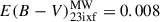 mag by querying the NASA/IPAC NED5 Galactic Extinction Calculator, based on the extinction map derived from Schlafly & Finkbeiner (2011). Reddening due to the host galaxy was estimated as
 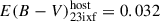 mag according to the equivalent width of the Na I D absorption lines measured from the high-resolution spectra of SN 2023ixf (Smith et al. 2023; Teja et al. 2023; Zhang et al. 2023) and the empirical relation derived between the line width and the dust reddening (Poznanski et al. 2012). Thus, the total reddening is estimated as
 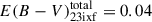 mag.
mag.
3.1. Light curves
After correcting for the Galactic and host-galaxy extinction, the UuBgVrizJHK-band light curves of SN 2023ixf are presented in Fig. 1, covering phases from 3 to 625 days after the explosion. A more thorough investigation of the photometric properties within the first hours to a few days is presented by Li et al. (2024). The V light curve of SN 2023ixf indicates a rise of ∼6 days before a peak magnitude of MVpeak = −18.0 ± 0.1 is reached. This rise time is at the short end of the distribution derived for the SN II population (González-Gaitán et al. 2015; Valenti et al. 2016). The high peak luminosity places SN 2023ixf near the bright end of SNe II as illustrated by detailed sample analyses (e.g., Anderson et al. 2014; Valenti et al. 2016; de Jaeger et al. 2019).
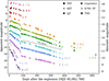 |
Fig. 1. Optical and NIR light curves of SN 2023ixf. Open circles mark the early g-, V-, and r-band light curves from Li et al. (2024). The dashed black line represents the decline expected for 56Co decay. |
Following Anderson et al. (2014) and using the V light curve of SN 2023ixf, we derived the s1 and s2 parameters: 3.35 ± 0.13 and 1.93 ± 0.10 mag per 100 days, respectively. They describe the magnitude decline rate measured from the time between the peak luminosity and the start of the linearly declining plateau (s1) and the magnitude decline rate when the SN has settled on its plateau phase (s2). These derived results are consistent with those measured by Zheng et al. (2025). Bersten et al. (2024) measured the s1 and s2 parameters of SN 2023ixf using the bolometric light curve. While our estimate of s2 is consistent with that reported by Bersten et al. (2024), our value of s1 is smaller. These results indicate an overall steeper decline compared to the corresponding mean values measured from the sample of Anderson et al. (2014), which are 2.65 mag and 1.47 mag per 100 days, respectively.
After ∼70 days, the V light curve of SN 2023ixf shows a transition from the plateau phase to the radioactive tail. During the phase between 100 and 300 days after the explosion, the V-band decline rate is measured to be 1.23 ± 0.01 mag (100 d)−1. Such a rate appears to be faster than that expected for the 56Co→56Fe decay, ∼0.98 mag (100 d)−1, as shown in Fig. 1. This indicates that γ-ray photons are not fully trapped inside the ejecta at this late phase.
3.2. Comparison of light curves
In Fig. 2 we compare the absolute V light curve of SN 2023ixf with those of a selected sample of well-studied Type II SNe, including Type IIP SNe 1999em (Leonard et al. 2002) and 2017gmr (Andrews et al. 2019), Type IIP/L SN 2013ej (Huang et al. 2015), Type II short-plateau SN 2006ai (Hiramatsu et al. 2021), and Type IIL SNe 1980K (Buta 1982) and 1990K (Cappellaro & Danziger 1995). All light curves have been corrected for extinction in both the host galaxy and the Milky Way.
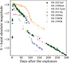 |
Fig. 2. Absolute V-band light curve of SN 2023ixf compared to those of the Type IIP/IIL SNe 1999em (Leonard et al. 2002), 2017gmr (Andrews et al. 2019), 2013ej (Huang et al. 2015), 2006ai (Anderson et al. 2014), 1980K (Buta 1982), and 1990K (Cappellaro & Danziger 1995). All magnitudes have been corrected for the host and the Galactic extinction components. |
The V light curve of SN 2023ixf shows a brighter absolute peak magnitude and shorter plateau compared to that of the prototypical SN IIP SN 1999em. A shorter and less prominent plateau can also be identified in the light curves of SN 2006ai and Type IIP/IIL SN 2013ej (Bose et al. 2015). The short-plateau Type II SN 2006ai, as discussed by Hiramatsu et al. (2021), is indicative of having a less massive H-rich envelope in its progenitor compared to that of normal SNe IIP (Hillier & Dessart 2019). The V light curves of Type IIL SNe 1980K and 1990K exhibit a much faster and more linear post-peak decline than that of SN 2023ixf during the plateau phase. Based on the comparison results discussed above, we suggest that SN 2023ixf is best described as a transitional object between Type IIP and IIL in terms of post-peak photometric evolution.
3.3. Pseudo-bolometric light curves
We calculated pseudo-bolometric light curves based on the multiband photometry. Since the light curves in different bands have different temporal coverage, we constructed pseudo-bolometric light curves using three different band coverages: UuBgVrizJHK, UuBgVriz, and BgVriz. To obtain the photometric data of different filters at comparable phases, the light curves were fitted using Gaussian process regression. We first estimated the SEDs from the photometric data, and then the SEDs were integrated to derive the pseudo-bolometric luminosity. Uncertainties were estimated through a Monte Carlo resampling of the light curves based on the photometric errors. The pseudo-bolometric light curves of SN 2023ixf are presented in Fig. 3.
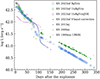 |
Fig. 3. Pseudo-bolometric light curves of SN 2023ixf established with photometry in different wavebands and only the V band. Comparisons with SN 2013ej (Yuan et al. 2016), SN 2006ai (Hiramatsu et al. 2021), and SN 1999em (Valenti et al. 2016) are also included. |
During the plateau and post-plateau phases, the V-band light curve of Type II/IIP SNe provides a good proxy for the bolometric evolution. This was characterized in detail by Bersten & Hamuy (2009), who found a root-mean-square scatter of ∼0.11 mag between the V-band and bolometric light curves. When settling to the radioactive-decay tail, the SN luminosity (in units of erg s−1) can be expressed as
![Mathematical equation: $$ \begin{aligned} {\log }\,L_{\rm t} = -0.4 [BC + V_{\rm t} - A(V) - 11.64] + {\log }_{10}(4\,\pi \,D^2), \end{aligned} $$](/articles/aa/full_html/2025/11/aa55030-25/aa55030-25-eq5.gif) (1)
(1)
where Vt is the V-band magnitude measured at t ≈ 90 days after the explosion, AV represents the V-band extinction along the line of sight (0.12 mag), D is the distance in cm, and BC denotes the bolometric correction, which has been estimated as −0.70 ± 0.02 mag (Bersten & Hamuy 2009) for the tail luminosity. We therefore adopted Eq. (1) to convert the V-band photometry of SN 2023ixf after day 90 to the bolometric light curve and plot it in Fig. 3.
As shown in Fig. 3, comparison between the pseudo-bolometric light curves constructed from the UuBgVriz and BgVriz bands reveals that the U/u band makes a significant contribution to the pseudo-bolometric luminosity in the first month, but the contribution becomes negligible during the plateau phase. In contrast, the comparison between the UuBgVrizJHK and UuBgVriz pseudo-bolometric light curves indicates that the NIR contribution is negligible during the first ten days but gradually increases thereafter. We also compared the bolometric light curve of SN 2023ixf with that of SNe 2013ej (Yuan et al. 2016) and 2006ai (Hiramatsu et al. 2021). Adopting a distance of 11.7 Mpc (Leonard et al. 2003), we calculated the UBVRI pseudo-bolometric light curve of SN 1999em (Leonard et al. 2002; Elmhamdi et al. 2003) using the method described above. The pseudo-bolometric light curve of SN 2023ixf shows a steeper plateau compared to SN 1999em, consistent with the V-band light-curve comparison presented in Sect. 3.2.
4. Spectroscopic evolution
4.1. Optical spectroscopy
In Fig. A.1 we present the spectral time series of SN 2023ixf observed by XLT, Copernico, GT, NOT, and LJT from days 3 to 324. All spectra are corrected for the redshift z = 0.000804 of its host galaxy (Riess et al. 2022) and de-reddened adopting a total line-of-sight extinction  mag.
mag.
Narrow emission lines including H, He II, and C IV remain prominent within the first three days after the explosion. The “flash features” at high excitation states arise from the shock-ionized species in the CSM shell in close vicinity of the exploding progenitor. This material was most likely expelled by pre-explosion instabilities in the years leading up to the terminal SN explosion, and the spectral signatures reflect the surface composition of the dying progenitor and trace the explosion and shock physics of the SN. Comprehensive analyses of the intra-night spectroscopic evolution of SN 2023ixf starting from day 1 has been carried out by Bostroem et al. (2023), Zheng et al. (2025), Hiramatsu et al. (2023), Smith et al. (2023), Teja et al. (2023), and Zhang et al. (2023). As illustrated in Fig. A.1, the flash features superimposed on the blue continuum persist for the first eight days.
Broad P Cygni profiles emerged for spectral lines of Ba II, Fe II, Sc II and Na I after the flash features were gone. A prominent Hα P Cygni line is seen after approximately day 20, indicating that the emission is dominated by the expanding H-rich envelope of the ejecta. Absorption on the blue side of Hα at ∼13 000 km s−1 appears at ∼20 d and disappears at ∼90 d. This notch was previously attributed to the high-velocity component of Hα (Leonard et al. 2002; Baron et al. 2000) or Si IIλ6355 (Pastorello et al. 2006; Valenti et al. 2014). The blue continuum diminishes as the SN enters the nebular phase.
At about 90 days after explosion, the photosphere recedes through the H envelope. The absorption component of the P Cygni profile of Hα disappears and forbidden metal emission lines of [O I] λ5577, [O I] λλ6300, 6364, [Ca II] λλ7291, 7323, and the Ca II NIR triplet emerge and start to dominate the spectra. Na Iλλ5890, 5896, [O I] λλ6300, 6364, Hα, and [Ca II] λλ7291, 7323 all show multi-peak profiles after about day 100, as discussed in detail in Sect. 4.7.
4.2. Comparison with other SNe II
Figure 4 compares the spectra of SN 2023ixf with those of other well-studied SNe IIP/L at similar epochs, namely SNe 2013ej6 (Valenti et al. 2014; Yuan et al. 2016; Huang et al. 2015), the typical Type IIP SN 1999em (Leonard et al. 2002), SN 2017gmr (Andrews et al. 2019), and SN 2006ai (Hiramatsu et al. 2021). All spectra were corrected for the redshift, as well as for host-galaxy and Galactic extinctions.
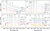 |
Fig. 4. Spectra of SN 2023ixf at days ∼5 (a), 40 (b), 150 (c), and 330 (d) compared to that of the Type IIP/L SNe 2013ej (Valenti et al. 2014; Yuan et al. 2016; Huang et al. 2015), 1999em (Leonard et al. 2002), 2017gmr (the spectrum at day 312 is binned; Andrews et al. 2019), and 2006ai (Hiramatsu et al. 2021) at similar phases. In each panel, major spectral features are marked by vertical dashed lines. For a better display, all spectra were shifted arbitrarily and presented in a logarithmic scale. |
As presented in Fig. 4a, while other comparison SNe have already developed broad P Cygni profiles of the Balmer lines, the spectrum of SN 2023ixf is still characterized by weak flash lines atop a blue continuum. The long-lived narrow flash features indicate that the process of the ejecta engulfing the CSM persists for the first eight days. Such an extended flash-ionization phase is significantly longer compared to the ∼5 day maximum duration observed in most CCSNe (Bruch et al. 2023), indicating more extreme CSM conditions.
Figure 4b shows a comparison of the spectrum of SN 2023ixf at day 42 with the other SNe at similar phases. SN 2023ixf presents a shallower Hα P Cygni absorption than others. Gutiérrez et al. (2014, 2017) found that the smaller ratio of absorption to emission of Hα is correlated with brighter and faster declining light curves. The shallower absorption component may imply a deficit in absorbing material at high velocities, which may naturally be reproduced by a rather steep density gradient in the H envelope. A lower envelope mass retained before the explosion can also contribute to the smaller ratio of the absorption to emission of Hα (Gutiérrez et al. 2014, 2017; Faran et al. 2014; Hiramatsu et al. 2021). Hillier & Dessart (2019) proposed that the interaction between the ejecta and CSM could also produce a weak or no Hα absorption. In addition, SN 2023ixf has fewer and shallower metal lines than SN 1999em.
Comparison of the day 150 spectrum of SN 2023ixf with those of other SNe is presented in Fig. 4c. While others still exhibit a P Cygni profile of Hα, the Hα absorption has already disappeared in SN 2023ixf. SN 2023ixf has more prominent [O I] λ5577, [O I] λλ6300, 6364, and [Ca II] λλ7291, 7323 lines compared to other SNe. The early appearance and strong emission of [O I] may hint that its progenitor was partially stripped before the explosion (Elmhamdi 2011). The Ca II NIR triplet of SN 2023ixf is comparable to that of SN 2017gmr but stronger than that of SN 1999em.
The comparison of the day 328 spectrum is shown in Fig. 4d. SN 2023ixf, SN 1999em, and SN 2017gmr all exhibit a double-peaked [O I] λλ6300, 6364 profile, but SN 2013ej has single-peaked [O I]. While the line profiles of SN 2023ixf, SN 2013ej, and SN 2017gmr are overall similar, their light curves show significant differences from each other (Fig. 2).
4.3. Metallicity
The line strengths of some metals measured during the photospheric phase were found to be correlated with the metallicity of their progenitors for SNe IIP/IIL (Dessart et al. 2014). For instance, the pseudo-equivalent width (pEW) of Fe IIλ5018 can be regarded as a metallicity indicator. The measured pEWs of Fe IIλ5018 of SN 2023ixf from the spectra between approximately days 50 and 70 and those of the models are presented in Fig. 5. The time interval was chosen to represent the mid-to-late plateau phase, during which the photosphere still probes the H envelope of the progenitor (Dessart et al. 2014). Without contamination through the outward chemical mixing from the inner core, the strengths of metal lines measured at the outer part of the SN ejecta can reflect the chemical content of the progenitor. As the photosphere of SN 2023ixf recedes into its inner He-rich core after t ≈ 70 days as indicated by the termination of the plateau phase (Fig. 1), comparison of the observations with the model can be made up to about day 70.
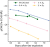 |
Fig. 5. pEW of Fe IIλ5018 in SN 2023ixf compared with the models presented by Dessart et al. (2014). The 0.4, 1, and 2 × Z⊙ models are shown by the color-coded lines (see the legend). |
From Fig. 5, one can see that the metallicity of SN 2023ixf falls into the range (0.4−1) Z⊙. We remark that one should remain cautious about the inferred range of the metallicity, as the reference models were constructed for SNe IIP with a prominent light-curve plateau, while both the photometric and spectroscopic properties of SN 2023ixf show close resemblances with Type IIL SNe.
4.4. Expansion velocity
Simulations of SN atmospheres based on the nonlocal thermodynamic equilibrium (non-LTE) CMFGEN model (Hillier & Miller 1998) suggest that the photospheric velocity of SNe II can be well traced by the absorption minimum of the Fe IIλ5169 feature (vFe; Dessart & Hillier 2005). We measured the absorption minima of Fe IIλ5169 in SN 2023ixf. At t ≈ 100 d, the profile of Fe IIλ5169 no longer follows a Gaussian profile, perhaps owing to line blending, so the velocity is not measured thereafter. The velocity evolution of SN 2023ixf is shown in Fig. 6, together with those measured for the Type IIP SNe 1999em (Takáts & Vinkó 2012) and 2005cs (Takáts & Vinkó 2012), the Type IIP/IIL SN 2013ej (Huang et al. 2015), and the Type II short-plateau SN 2006ai (Hiramatsu et al. 2021).
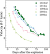 |
Fig. 6. Comparison of the evolution of the Fe IIλ5169 velocity of SN 2023ixf with those of SNe 2013ej, 1999em, 2005cs, and 2006ai. |
A comparison of the Fe IIλ5169 velocity evolution of SN 2023ixf and other Type IIP/L SNe suggests that the former also follows an exponential-like decline as observed in the other presented cases. SN 2023ixf displays an ejecta velocity evolution similar to that measured for SNe 2013ej and 2006ai, significantly higher than that of the normal SN IIP 1999em (Elmhamdi et al. 2003; Utrobin et al. 2017) and the sub-luminous SN IIP 2005cs (Pastorello et al. 2006, 2009). The velocities of sub-luminous and normal SNe II being different may be indicative of the associated total energy and the debris of the SN explosion. For example, the former and the latter are thought to be linked to the O-Ne-Mg core and Fe core from progenitors with lower (∼8−10 M⊙) and higher masses (≳10 M⊙), respectively (Fraser et al. 2011; Janka 2012). Faster expansion velocities of SNe IIP are considered to be linked with higher explosion energies (Dessart et al. 2010; Gutiérrez et al. 2017; Martinez et al. 2022b).
4.5. Distance
The expanding photosphere method (EPM) provides an independent estimate of the distance to a SN based on a comparison between the physical and angular radii of its photosphere, denoted by r and θ, respectively (Kirshner & Kwan 1974). The former can be calculated by multiplying the expansion velocity of the photosphere (vphot) by the time elapsed since the SN explosion (t − t0), and the latter can be used to estimate the distance to the SN (D) through direct geometric calculation,
 (2)
(2)
We adopted the velocities measured from the absorption minimum of Fe IIλ5169 to represent vphot, as discussed in Sect. 4.4. Following the prescriptions described by Leonard et al. (2002) and Dessart & Hillier (2005), the comparison between the synthetic magnitude calculated from a blackbody spectrum and the photometry of the SN in a given bandpass can be facilitated by minimizing the quantity ϵ, and θ can be derived via
![Mathematical equation: $$ \begin{aligned} \epsilon = \sum \limits _{\rm BVI} {\left\{ m_{\rm BVI} - A_{\rm BVI} + 5\,{\log }\,\theta + 5\,{\log }\,[\zeta (T_{\rm c})] - b_{\rm BVI}(T_{\rm c})\right\} }^2, \end{aligned} $$](/articles/aa/full_html/2025/11/aa55030-25/aa55030-25-eq8.gif) (3)
(3)
where bBVI is the synthetic broadband magnitude of the Planck function with temperature Tc. The dilution factor, ζ, corrects the difference between the thermalization and photospheric radii, the former of which is determined by the blackbody temperature (Eastman et al. 1996; Hamuy et al. 2001). We converted the i-band magnitude to Johnson I using the Lupton (2005) color transformations7.
Minimization of the quantity ϵ was achieved through a Markov chain Monte Carlo approach. Upon the determination of θ and vphot, the distance to the SN was then carried out based on Eq. (2). The priors of parameters are assumed to be uniform. Jones et al. (2009) show a clear departure from linearity between θ/v versus t after t ≈ 45 − 50 days, likely caused by the progressively emerging spectral lines that deviate the continuum emission of a blackbody (Dessart & Hillier 2005). Therefore, we restricted the EPM analysis to before this phase.
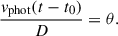
Based on the EPM approach, we estimated the distance to M 101 to be  Mpc (
Mpc ( mag). The distance derived using the standard candle method (Zheng et al. 2025) is 28.67 ± 0.14 mag. Distances measured with Cepheids range from 6.19 to 8.99 Mpc (Mager et al. 2013; Macri et al. 2001), while those measured with SNe Ia range from 5.92 to 7.52 Mpc (Matheson et al. 2012; Munari et al. 2013). Therefore, our result is consistent with distances measured from other methods.
4.6. Hα profile during the nebular phase
During the photospheric phase, the Hα line of SN 2023ixf is characterized by a P Cygni profile, as shown in Fig. A.1. After t ≈ 90 days, the absorption component of Hα is diminished and the emission component of Hα starts to develop into a double-peaked profile. The evolution of the nebular-phase Hα profile, normalized by the pseudo-continuum, is shown in Fig. 7 (note that the 407 day spectrum has been published by Zheng et al. 2025). It is evident that the Hα line of SN 2023ixf developed a complex profile when entering the nebular phase. For instance, at t ≈ 189 days, the profile exhibits a multi-peak structure with emission peaks ranging from ∼ − 1500 km s−1 (blueshifted) to ∼ + 1500 km s−1 (redshifted). The blueshifted component appears stronger than the redshifted counterpart. Such an asymmetric Hα profile was also observed in other SNe II, such as SN 1999em (Leonard et al. 2002), SN 2013ej (Huang et al. 2015), and SN 2017gmr (Andrews et al. 2019), and has been attributed to bipolar distribution of Ni. The suppressed redshifted component could instead be attributed to dust formation, as first proposed for the late-time spectral evolution of SN 1987A (Lucy et al. 1989). On-site dust formation has also been reported in some CCSNe, such as SN 2006jc (Smith et al. 2008), SN 1999em (Elmhamdi et al. 2003), SN 2010jl (Zhang et al. 2012), and SN 2018hfm (Zhang et al. 2022), most likely taking place in a cold dense shell between the forward-shock and reverse-shock fronts (Chugai 2001; Chugai et al. 2004; Dessart et al. 2009). In SN 2023ixf, further evidence of dust formation can be inferred from the flux excesses in the NIR and mid-infrared (MIR) light curves taken beyond ∼120 days (Singh et al. 2024; Van Dyk et al. 2024b). In particular, the MIR light curve displays a prominent brightening at day ∼210 at ∼4.6 μm, which can be explained by the emergence of line emission from the 1−0 vibrational band of carbon monoxide (CO) at 4.65 μm.
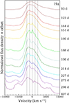 |
Fig. 7. Temporal evolution of the Hα profile from days 93 to 298. The vertical dashed black lines mark the rest-frame velocities of −2000, −1000, 0, +1000, and +2000 km s−1. |
We also note that starting from t ≈ 90 days, a notch on the red shoulder of the Hα line started to develop, indicating the contribution from a flat-topped component underlying the emission feature (Fig. A.1). As shown by the t ≈ 93 day spectrum in Fig. 7, the box-shaped continuum extends to a velocity range of ∼5000 − 8000 km s−1 with respect to the rest-frame zero velocity of Hα. Such a boxy-shaped emission feature provides signatures of strong interaction between the expanding ejecta and shell-like CSM. The edges of the emission indicate the expanding velocity of the ejecta (see, e.g., Dessart & Hillier 2022), which is 8000 km s−1. Taking into account that this signature of interaction emerges at ∼90 days after the explosion, the boxy-shaped emission suggests a CSM shell at a distance of ∼6.2 × 1015 cm. Assuming the CSM shell was produced by a typical red supergiant wind at a velocity of ∼10 km s−1, this material was expelled ∼200 yr before the explosion. A blueshifted peak at ∼ − 8000 km s−1 started to emerge at day 190, which shifted gradually to ∼ − 5000 km s−1 by t ≈ 400 days. The different profiles on the right and left sides of Hα above 5000 km s−1 may naturally be due to the presence of a spherically asymmetric dense shell. Furthermore, we note that the shoulder on the right side of the Hα profile persisted until day ∼150, and emerged again from roughly day 275. This may indicate a persisting interaction with multiple CSM shells. These shells may result from multiple episodes of mass loss that lead to SN 2023ixf at ≳200 yr before the explosion. These bumps might also be attributed to bipolar ejecta at the largest velocity interacting with the CSM (Smith et al. 2012). The narrow component at 0 km s−1 appearing at days 160−189 might be from the host galaxy, as weak [S II] λλ6716, 6731 lines are observed at the same epoch.
4.7. Temporal evolution of the spectral line profiles in the nebular phase
For the purpose of investigating the temporal evolution of the morphology of several prominent spectral features in the nebular phase of SN 2023ixf, we normalized the spectra by the pseudo-continuum. Spectral lines of Na Iλλ5890, 5896, [O I] λλ6300, 6364, Hα, and [Ca II] λλ7291, 7323, spanning days 132 to 407, are shown in Fig. 8. We inspected the line velocities of [O I] λλ6300, 6364 and [Ca II] λλ7291, 7323 with respect to their rest-frame wavelengths.
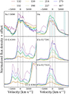 |
Fig. 8. Temporal evolution of the spectral line profiles centered at the rest-frame wavelengths of Na Iλ5890, 5896, [O I] λ6300, [O I] λ6364, Hα, [Ca II] λ7291, and [Ca II] λ7323, as labeled in each subpanel. All spectra are presented in velocity space. Three vertical dashed black lines mark the rest-frame velocities of −1500, 0, and +1500 km s−1. The dotted blue lines mark the [N II] λλ6548, 6583 and [S II] λλ6716, 6731 emission lines from an H II region in the host galaxy. |
First, as the photosphere progressively recedes, the emission component of the Na I D λλ5890, 5896 doublet emerges in the spectra. A double-peaked emission profile centered at zero velocity can be identified, with a nearly constant pEW over time. The blueshifted and redshifted components peak at ∼−1500 and +1500 km s−1, respectively. As lines from [O I] and [Ca II] strengthen with time with respect to the pseudo-continuum, Hα diminishes gradually. Second, the Hα line also exhibits a dual-peaked morphology as seen from the Na Iλλ5890, 5896 doublet, which also peaked at ∼−1500 and +1500 km s−1, respectively. Third, the velocity profiles centered at 6300 and 6364 Å suggest that both doublets display a blueshifted component at −1500 km s−1. A similar characterization can also be inferred for the [Ca II] λλ7291, 7323 profile. Finally, a redshifted component can be identified from the shoulders in the red-side profiles of the [Ca II] doublet at a velocity of ∼+1500 km s−1. We tentatively identify a redshifted component in the [O I] lines as they are likely blended with the blue wing of Hα.
In summary, the zoom-in of the pseudo-continuum-normalized profiles of the presented lines of interest exhibits a more prominent component shifted by ∼1500 km s−1 to the blue, and another, weaker component shifted by ∼1500 km s−1 to the red. The dual-peaked spectral line profiles of SN 2023ixf might hint at an aspherical distribution of the ejecta (Utrobin et al. 2021; Chugai et al. 2005).
4.8. Near-infrared spectroscopy
In Fig. 9 we present a total of seven NIR spectra of SN 2023ixf obtained with TNG+NICS. At ∼4 days past explosion, the spectrum exhibits a weak narrow emission line of Pβ 1.282 μm superimposed on the continuum. Seven days later, Pβ disappears and no prominent line can be identified. At ∼30 days after explosion, Pβ and Bγ 2.165 μm appear and strengthen over time. Pβ develops a P Cygni profile at 49 d. Mg I 1.503 μm and Si I 1.203 μm appear at about 70 d. Pα 1.875 μm is seriously compromised by the telluric absorption. No CO overtone at 2.3 μm is discernible.
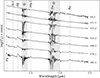 |
Fig. 9. NIR spectra of SN 2023ixf observed by TNG from t ≈ 4 to 80 days after the explosion. Phases are indicated to the right of each spectrum. Several prominent spectral lines are marked with vertical dashed lines. Telluric lines are shown with crossed circles and gray shading. |
We compared the NIR spectra of SN 2023ixf with those of SN 2013ej (Davis et al. 2019) at similar phases (Fig. 10). The narrow Pβ observed in SN 2023ixf at t ≈ 4 days cannot be discerned in SN 2013ej at t ≈ 5 days. The spectra of SN 2023ixf show much stronger and broader Mg I 1.503 μm and Si I 1.203 μm than SN 2013ej.
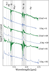 |
Fig. 10. Comparison of the NIR spectra of SN 2023ixf with those of SN 2013ej at similar phases. Several prominent spectral features are marked by dashed lines, and telluric absorption is shown with crossed circles and gray shading. |
5. Discussion
5.1. 56Ni mass
56Ni is synthesized during the SN explosion. The trapping of the γ-rays produced in the decay chain 56Ni→56Co→56Fe is the main power source of the radioactive-tail luminosity of SNe. Therefore, the bolometric flux of the tail can be utilized to estimate the amount of radioactive 56Ni synthesized in the SN explosion.
As shown in Fig. 1 and discussed in Sect. 3.1, the radioactive tail of SN 2023ixf declines faster than the decay of 56Co assuming full trapping of gamma-ray photons. Therefore, we infer an incomplete trapping of γ-ray photons, which could be attributed to the decreasing photon diffusion time as the SN ejecta expand and become more transparent. Accounting for the γ-ray leakage, the luminosity from solely the 56Ni→56Co→56Fe decay chain can be fitted following the prescription of Yuan et al. (2016):
 (4)
(4)
where L is the bolometric luminosity, mNi gives the mass of 56Ni synthesized in the SN explosion, t represents the time since explosion, and tCo and tNi are the e-folding times of 56Co and 56Ni (111.4 and 8.8 days, respectively). The term t1 represents the characteristic time when the γ-ray optical depth of the ejecta drops to unity. This characteristic timescale is determined by the average γ-ray opacity, the total mass of the ejecta, and the kinetic energy of the SN. The t−2 dependence of the optical depth is due to the decreasing column density as the SN ejecta undergo homologous expansion (Clocchiatti & Wheeler 1997).
As described in Sect. 3.3, the pseudo-bolometric light curve is converted from the V-band magnitudes obtained during days 90 to 350, and the mass of 56Ni synthesized in the ejecta is estimated by fitting Eq. (4) assuming incomplete trapping of X-rays and electrons/positrons. The best fit to the single radioactive decay chain model suggests mNi = 0.059 ± 0.001 M⊙ and t1 = 312.9 ± 4.6 days. The derived nickel mass is consistent with that calculated by Singh et al. (2024) and Bersten et al. (2024). Adopting a distance of 11.7 Mpc (Leonard et al. 2003) and using the V-band photometry from Leonard et al. (2002), we also estimated the 56Ni mass of SN 1999em following the method described above. The derived 56Ni mass of SN 1999em is 0.064 M⊙, comparable to that of SN 2023ixf.
5.2. Comparison of nebular spectra with theoretical models
While the SN expands, its deep interior becomes visible as a result of decreased column densities and removal of free elections owing to recombination. Spectra at the nebular phase are hence free from photospheric absorption lines and are typically dominated by emission features. Nebular-phase spectra of CCSNe thus reveal the physical conditions of a variety of nuclear burning zones, enabling unambiguous model diagnostics.
In Fig. 11 we compare the t ≈ 275 day spectrum of SN 2023ixf with a set of theoretical models with ZAMS masses of 12, 15, and 19 M⊙ at similar phases (at t ≈ 250 day; Jerkstrand et al. 2014). The spectrum of SN 2023ixf is flux calibrated using interpolated photometry. For comparison purposes, all spectra have been scaled with respect to the total flux integrated over the observed wavelength range. We note that the profile of the [O I] λλ6300, 6364 doublet of SN 2023ixf is in good agreement with that calculated for the 19 M⊙ model. However, the [Ca II] λλ7291, 7323 doublet of SN 2023ixf is significantly stronger than that of the models, and Hα of SN 2023ixf is much weaker than the modeled profiles. Note that the Hα, [Ca II] λλ7291, 7323, and Ca II NIR triplet are mainly formed in the outer layers of the H-rich ejecta. Consequently, their line strengths are dependent on both the pre-explosion mass loss and the distribution of the associated elements themselves. The latter may indicate the degree of outward mixing of Ni-rich ejecta.
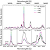 |
Fig. 11. Comparison of the nebular-phase spectrum of SN 2023ixf obtained at day 275 and the non-LTE model spectra at day 250 for CCSNe with ZAMS masses of 12, 15, and 19 M⊙. The subpanels in the lower row zoom in on the [O I] + Hα, [Ca II], and Ca II NIR triplet regions. |
5.3. Progenitor mass estimation
Since oxygen is one of the products of a series of hydrostatic burning phases, the amount of oxygen in the ejecta increases with ZAMS mass. Since oxygen also acts as the fuel for calcium production during the explosive burning phase, the strength of [O I] λλ6300, 6364 s and the [Ca II]/[O I] flux ratio provide sensitive indicators of the ZAMS mass of the progenitor of CCSNe (Fransson & Chevalier 1989; Jerkstrand et al. 2012, 2014, 2015). Our spectra of SN 2023ixf have been scaled to match the photometry at different bandpasses. The photometry is interpolated or extrapolated to get the corresponding values at the phases the spectra were taken. The spectrum at day 298 is constructed from the spectra taken on days 297.2 and 298.1.
To derive the progenitor mass of SN 2023ixf, we first estimated the continuum underlying the [O I] line by connecting the visually inspected blue end of the [O I] and the red end of Hα. This “pseudo-continuum” represented by such a line segment is then subtracted from the spectral region of interest, as shown in Fig. B.1. Second, a multicomponent Gaussian function is used to fit the features of the [O I] + Hα emission complex between days 275 and 407. For the measurement of each phase, we calculated the area below the Gaussian functions that fit the λλ6300, 6364 feature to obtain the [O I] luminosity. Finally, we divided the time series of [O I] luminosity by the intensity integrated in the range 4800−8900 Å of the same spectrum. The aim of the last step of normalization is to remove the dependence of [O I] luminosity on the γ-ray trapping. The selected wavelength range is similar to that adopted by Anderson et al. (2018) and Fang et al. (2025).
In Fig. 12 we present the fraction of the [O I] flux of SN 2023ixf at days 275, 298, and 407. The same calculation was also carried out for a series of model spectra with different progenitor ZAMS masses as computed by Jerkstrand et al. (2014). The [O I] percentages of SN 2023ixf estimated in the nebular phase fall in the progenitor mass range of 15−19 M⊙, consistent with the results of Fang et al. (2025), Jencson et al. (2023), Niu et al. (2023), Qin et al. (2024), and Zheng et al. (2025). Ferrari et al. (2024) compared the [O I]/[Ca II] flux ratio of SN 2023ixf with that measured from the models in Jerkstrand et al. (2014), and a ZAMS progenitor mass between 12 and 15 M⊙ is derived.
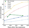 |
Fig. 12. Temporal evolution of the measured [O I] λλ6300, 6364 flux for SN 2023ixf as a percentage of the total optical flux, along with that of the modeled spectra presented by Jerkstrand et al. (2014). |
We remark that the [O I] flux estimated based on multicomponent Gaussian fitting may introduce additional systematic uncertainties that are difficult to characterize. For example, any departure from spherical symmetry would alter the shape of the line profile. Additionally, dust formation may alter the line asymmetry by suppressing the flux in the blue wing and creating an extended profile in the red wing. A box-shaped underlying continuum of Hα blended with [O I] may affect the estimation of the flux of [O I]. However, as the measurements of the data and the models were carried out following an identical procedure, and the intensity-normalized [O I] flux measured for various progenitor models confirms the trend of increasing mass of the progenitor, we suggest that the ZAMS mass estimated for SN 2023ixf based on the [O I] flux remains robust.
6. Conclusion
We have presented extensive optical and NIR photometric and spectroscopic observations of SN 2023ixf spanning 3−625 days after the explosion. The narrow flash lines of SN 2023ixf persist for a few days after the explosion. These features favor the presence of a radially confined CSM shell around the progenitor (Bostroem et al. 2023; Hiramatsu et al. 2023; Smith et al. 2023; Teja et al. 2023; Zhang et al. 2023; Zheng et al. 2025). SN 2023ixf reached a V-band absolute peak magnitude of MV = −18.1 ± 0.1 mag at about 6 days after the explosion, which is at the bright end of what is typical for SNe II (Anderson et al. 2014; Valenti et al. 2016; de Jaeger et al. 2019). The rise time is on the short end of what is typical (González-Gaitán et al. 2015; Valenti et al. 2016). SN 2023ixf exhibits a slanted plateau feature (∼1.47 mag per 100 d in V), placing it within the transitional regime between SNe IIP and SNe IIL. A comparison with well-modeled SNe II suggests that SN 2023ixf might have a low H envelope mass (Hiramatsu et al. 2021). However, the slope of the plateau can also be affected by nickel mixing (Bersten et al. 2011) and/or the interaction of SN ejecta with an extended CSM (Morozova et al. 2017, 2018).
The photospheric velocities of SN 2023ixf are higher than those of typical SNe IIP, suggesting a higher ejecta kinetic energy (Dessart et al. 2010; Gutiérrez et al. 2017; Martinez et al. 2022b). The metallicity of SN 2023ixf derived from the pEW of Fe II during the photospheric phase falls between 0.4 Z⊙ and 1 Z⊙. Using EPM, we estimate the distance to the SN to be  Mpc.
Mpc.
Taking the incomplete trapping of the γ-rays into account, we used the radioactive-tail luminosity of SN 2023ixf to calculate the mass of 56Ni synthesized during the SN explosion, 0.059 ± 0.001 M⊙. This result is consistent with the values derived from hydrodynamic light-curve modeling, namely 0.05 M⊙ (Bersten et al. 2024) and 0.06 M⊙ (Singh et al. 2024). We compared the percentage of [O I] flux of SN 2023ixf with that of the synthetic spectra in Jerkstrand et al. (2014), and from this estimated the mass of the progenitor to be 15−19 M⊙, which is consistent with the results suggested from HST and Spitzer archival images (Jencson et al. 2023; Soraisam et al. 2023; Qin et al. 2024; Niu et al. 2023). While the progenitor mass of SN 2023ixf is on the higher end of what is typical for SNe II (Morozova et al. 2018; Martinez et al. 2022a), its light-curve evolution suggests a relatively low hydrogen-rich envelope mass. This contrast may be due to the significant mass loss prior to its explosion. Ferrari et al. (2024) compared the [O I]/[Ca II] flux ratio of SN 2023ixf to that of the same nebular models and inferred a progenitor mass between 12 and 15 M⊙. This is lower than our result. However, the [Ca II] λλ7291, 7324 may be blended with [Fe II] λλ7155, 7453 and [Ni II] λλ7377, 7412, potentially affecting the flux-ratio measurement. The progenitor mass of SN 2023ixf has also been estimated through hydrodynamic modeling of its light curves, with estimated values ranging from 10 M⊙ (Singh et al. 2024) and 12 M⊙ (Bersten et al. 2024) to ≳17 M⊙ (Hsu et al. 2024). Moreover, Fang et al. (2025) recently found that the light curves of SN 2023ixf can be reproduced with a progenitor mass in the range 12−17.5 M⊙.
The emission lines of hydrogen, sodium, oxygen, and calcium exhibit double-peaked profiles during the nebular phase, hinting at an aspherical distribution of the ejecta. The box-shaped Hα profile extending up to 8000 km s−1 indicates interaction between the ejecta and CSM (Dessart & Hillier 2022). The different profiles on the blue and red sides of the Hα profile may be due to a spherically asymmetric CSM shell. The disappearance of the red shoulder of Hα at day ∼150 and its reappearance at day ∼275 might result from multiple episodes of mass loss ≳200 yr before the explosion.
Data availability
The full version of Table 1 is available at the CDS via https://cdsarc.cds.unistra.fr/viz-bin/cat/J/A+A/703/A168. The spectra presented in this paper are available on the Weizmann Interactive Supernova Data Repository (WISeREP; Yaron & Gal-Yam 2012).
IRAF is distributed by the National Optical Astronomy Observatories, which are operated by the Association of Universities for Research in Astronomy, Inc., under cooperative agreement with the U.S. National Science Foundation.
SNOoPY is a package for SN photometry using point-spread-function fitting and/or template subtraction developed by E. Cappellaro. A package description can be found at https://sngroup.oapd.inaf.it/snoopy.html
FOSCGUI is a graphical user interface (GUI) dedicated to extract the photometry and spectroscopy obtained with FOSC-like instruments. It was developed by E. Cappellaro. A package description can be found at https://sngroup.oapd.inaf.it/foscgui.html
This previously unpublished spectrum at 337 d is from A. V. Filippenko’s group at UC Berkeley. It was obtained on 26 June 2014 with the DEep Imaging Multi-Object Spectrograph (DEIMOS; Faber et al. 2003) on the 10 m Keck II telescope on Maunakea, with the long slit aligned at the parallactic angle (Filippenko 1982). The spectrum was reduced with standard IRAF routines (Silverman et al. 2012) and was flux calibrated using spectrophotometric standard stars.
Acknowledgments
The work of X.W. is supported by the National Natural Science Foundation of China (NSFC grants 12288102 and 12033003), and the Newcorner Stone Foundation, and the Mahuateng Foundation. A.R. acknowledges financial support from the GRAWITA Large Program Grant (PI P. D’Avanzo) and from PRIN-INAF 2022 “Shedding light on the nature of gap transients: from the observations to the models”. Y.-Z. Cai is supported by NSFC grant 12303054, the National Key Research and Development Program of China (grants 2024YFA1611603, 202501AS070078), the Yunnan Fundamental Research Projects (grant 202401AU070063), and the International Centre of Supernovae, Yunnan Key Laboratory (grant 202302AN360001). A.P., A.R., G.V., and I.S. are supported by PRIN-INAF 2022 project “Shedding light on the nature of gap transients: from the observations to the models”. J.Z. is supported by the National Key R&D Program of China with grant 2021YFA1600404, NSFC grants 12173082 and 12333008, the Yunnan Fundamental Research Projects (grants 202501AV070012, 202401BC070007 and 202201AT070069), the Top-notch Young Talents Program of Yunnan Province, the Light of West China Program provided by the Chinese Academy of Sciences, and the International Centre of Supernovae, Yunnan Key Laboratory (grant 202302AN360001). M.H. acknowledges the support from the Postdoctoral Fellowship Program of CPSF under Grant Number GZB20240376, and the Shuimu Tsinghua Scholar Program 2024SM118. A.V.F.’s group at U.C. Berkeley is grateful for financial support from the Christopher R. Redlich Fund, Gary and Cynthia Bengier, Clark and Sharon Winslow, Sanford Robertson (Y.Y. was a Bengier-Winslow-Robertson Postdoctoral Fellow when this work was started), and many other donors. We acknowledge the support of the staff of the Xinglong 80 cm telescope and the Xinglong 2.16 m telescope. This work was partially supported by the Open Project Program of the Key Laboratory of Optical Astronomy, National Astronomical Observatories, Chinese Academy of Sciences. This article is also based in part on observations made at the Observatorios de Canarias del IAC with the Telescopio Nazionale Galileo, operated on the island of La Palma by INAF at the Observatorio del Roque de los Muchachos, under program A47DDT3 (PI G. Valerin). Some of the data presented herein were obtained at the W. M. Keck Observatory, which is operated as a scientific partnership among the California Institute of Technology, the University of California, and NASA; the observatory was made possible by the generous financial support of the W. M. Keck Foundation. We thank Melissa Graham, Patrick Kelly, WeiKang Zheng, and Jon Mauerhan for assistance obtaining the Keck SN 2013ej spectrum.
References
- Ahumada, R., Allende Prieto, C., Almeida, A., et al. 2020, ApJS, 249, 3 [NASA ADS] [CrossRef] [Google Scholar]
- Anderson, J. P., González-Gaitán, S., Hamuy, M., et al. 2014, ApJ, 786, 67 [Google Scholar]
- Anderson, J. P., Dessart, L., Gutiérrez, C. P., et al. 2018, Nat. Astron., 2, 574 [NASA ADS] [CrossRef] [Google Scholar]
- Andrews, J. E., Sand, D. J., Valenti, S., et al. 2019, ApJ, 885, 43 [Google Scholar]
- Arcavi, I., Gal-Yam, A., Cenko, S. B., et al. 2012, ApJ, 756, L30 [NASA ADS] [CrossRef] [Google Scholar]
- Baffa, C., Comoretto, G., Gennari, S., et al. 2001, A&A, 378, 722 [NASA ADS] [CrossRef] [EDP Sciences] [Google Scholar]
- Barbieri, C., Bhatia, R. K., Bonoli, C., et al. 1994, SPIE Conf. Ser., 2199, 10 [Google Scholar]
- Barbon, R., Ciatti, F., & Rosino, L. 1979, A&A, 72, 287 [Google Scholar]
- Baron, E., Branch, D., Hauschildt, P. H., et al. 2000, ApJ, 545, 444 [Google Scholar]
- Bersten, M. C., & Hamuy, M. 2009, ApJ, 701, 200 [NASA ADS] [CrossRef] [Google Scholar]
- Bersten, M. C., Benvenuto, O., & Hamuy, M. 2011, ApJ, 729, 61 [NASA ADS] [CrossRef] [Google Scholar]
- Bersten, M. C., Orellana, M., Folatelli, G., et al. 2024, A&A, 681, L18 [NASA ADS] [CrossRef] [EDP Sciences] [Google Scholar]
- Bose, S., Sutaria, F., Kumar, B., et al. 2015, ApJ, 806, 160 [Google Scholar]
- Bostroem, K. A., Pearson, J., Shrestha, M., et al. 2023, ApJ, 956, L5 [NASA ADS] [CrossRef] [Google Scholar]
- Brennan, S. J., & Fraser, M. 2022, A&A, 667, A62 [NASA ADS] [CrossRef] [EDP Sciences] [Google Scholar]
- Bruch, R. J., Gal-Yam, A., Schulze, S., et al. 2021, ApJ, 912, 46 [NASA ADS] [CrossRef] [Google Scholar]
- Bruch, R. J., Gal-Yam, A., Yaron, O., et al. 2023, ApJ, 952, 119 [NASA ADS] [CrossRef] [Google Scholar]
- Buta, R. J. 1982, PASP, 94, 578 [CrossRef] [Google Scholar]
- Cappellaro, E., Danziger, I. J., della Valle, M., Gouiffes, C., & Turatto, M., 1995, A&A, 293, 723 [Google Scholar]
- Chugai, N. N. 2001, MNRAS, 326, 1448 [NASA ADS] [CrossRef] [Google Scholar]
- Chugai, N. N., Blinnikov, S. I., Cumming, R. J., et al. 2004, MNRAS, 352, 1213 [NASA ADS] [CrossRef] [Google Scholar]
- Chugai, N. N., Fabrika, S. N., Sholukhova, O. N., et al. 2005, Astron. Lett., 31, 792 [NASA ADS] [CrossRef] [Google Scholar]
- Clocchiatti, A., & Wheeler, J. C. 1997, ApJ, 491, 375 [Google Scholar]
- Davis, S., Hsiao, E. Y., Ashall, C., et al. 2019, ApJ, 887, 4 [NASA ADS] [CrossRef] [Google Scholar]
- de Jaeger, T., Zheng, W., Stahl, B. E., et al. 2019, MNRAS, 490, 2799 [NASA ADS] [CrossRef] [Google Scholar]
- Dessart, L., & Hillier, D. J. 2005, A&A, 439, 671 [NASA ADS] [CrossRef] [EDP Sciences] [Google Scholar]
- Dessart, L., & Hillier, D. J. 2011, MNRAS, 410, 1739 [NASA ADS] [Google Scholar]
- Dessart, L., & Hillier, D. J. 2022, A&A, 660, L9 [NASA ADS] [CrossRef] [EDP Sciences] [Google Scholar]
- Dessart, L., Hillier, D. J., Gezari, S., Basa, S., & Matheson, T. 2009, MNRAS, 394, 21 [NASA ADS] [CrossRef] [Google Scholar]
- Dessart, L., Livne, E., & Waldman, R. 2010, MNRAS, 408, 827 [NASA ADS] [CrossRef] [Google Scholar]
- Dessart, L., Gutierrez, C. P., Hamuy, M., et al. 2014, MNRAS, 440, 1856 [NASA ADS] [CrossRef] [Google Scholar]
- Eastman, R. G., Schmidt, B. P., & Kirshner, R. 1996, ApJ, 466, 911 [NASA ADS] [CrossRef] [Google Scholar]
- Ehgamberdiev, S. 2018, Nat. Astron., 2, 349 [NASA ADS] [CrossRef] [Google Scholar]
- Elmhamdi, A. 2011, Acta Astron., 61, 179 [NASA ADS] [Google Scholar]
- Elmhamdi, A., Danziger, I. J., Chugai, N., et al. 2003, MNRAS, 338, 939 [CrossRef] [Google Scholar]
- Faber, S. M., Phillips, A. C., Kibrick, R. I., et al. 2003, SPIE Conf. Ser., 4841, 1657 [Google Scholar]
- Fan, Y.-F., Bai, J.-M., Zhang, J.-J., et al. 2015, RAA, 15, 918 [Google Scholar]
- Fang, Q., Moriya, T. J., Ferrari, L., et al. 2025, ApJ, 978, 36 [NASA ADS] [CrossRef] [Google Scholar]
- Faran, T., Poznanski, D., Filippenko, A. V., et al. 2014, MNRAS, 445, 554 [NASA ADS] [CrossRef] [Google Scholar]
- Ferrari, L., Folatelli, G., Ertini, K., Kuncarayakti, H., & Andrews, J. E. 2024, A&A, 687, L20 [NASA ADS] [CrossRef] [EDP Sciences] [Google Scholar]
- Filippenko, A. V. 1982, PASP, 94, 715 [Google Scholar]
- Folatelli, G., Ferrari, L., Ertini, K., Kuncarayakti, H., & Maeda, K. 2025, A&A, 698, A213 [NASA ADS] [CrossRef] [EDP Sciences] [Google Scholar]
- Förster, F., Moriya, T. J., Maureira, J. C., et al. 2018, Nat. Astron., 2, 808 [CrossRef] [Google Scholar]
- Fransson, C., & Chevalier, R. A. 1989, ApJ, 343, 323 [NASA ADS] [CrossRef] [Google Scholar]
- Fraser, M., Ergon, M., Eldridge, J. J., et al. 2011, MNRAS, 417, 1417 [NASA ADS] [CrossRef] [Google Scholar]
- Fukugita, M., Ichikawa, T., Gunn, J. E., et al. 1996, AJ, 111, 1748 [Google Scholar]
- Gal-Yam, A., Arcavi, I., Ofek, E. O., et al. 2014, Nature, 509, 471 [CrossRef] [Google Scholar]
- González-Gaitán, S., Tominaga, N., Molina, J., et al. 2015, MNRAS, 451, 2212 [CrossRef] [Google Scholar]
- Gutiérrez, C. P., Anderson, J. P., Hamuy, M., et al. 2014, ApJ, 786, L15 [CrossRef] [Google Scholar]
- Gutiérrez, C. P., Anderson, J. P., Hamuy, M., et al. 2017, ApJ, 850, 90 [CrossRef] [Google Scholar]
- Hamuy, M. 2003, ApJ, 582, 905 [NASA ADS] [CrossRef] [Google Scholar]
- Hamuy, M., Pinto, P. A., Maza, J., et al. 2001, ApJ, 558, 615 [NASA ADS] [CrossRef] [Google Scholar]
- Henden, A. A., Templeton, M., Terrell, D., et al. 2016, VizieR Online Data Catalog: II/336 [Google Scholar]
- Hillier, D. J., & Dessart, L. 2019, A&A, 631, A8 [NASA ADS] [CrossRef] [EDP Sciences] [Google Scholar]
- Hillier, D. J., & Miller, D. L. 1998, ApJ, 496, 407 [NASA ADS] [CrossRef] [Google Scholar]
- Hiramatsu, D., Howell, D. A., Moriya, T. J., et al. 2021, ApJ, 913, 55 [CrossRef] [Google Scholar]
- Hiramatsu, D., Tsuna, D., Berger, E., et al. 2023, ApJ, 955, L8 [NASA ADS] [CrossRef] [Google Scholar]
- Hsu, B., Smith, N., Goldberg, J. A., et al. 2024, ApJ, submitted [arXiv:2408.07874] [Google Scholar]
- Hu, M., Wang, L., & Wang, X. 2025, ApJ, 984, 44 [Google Scholar]
- Huang, F., Li, J.-Z., Wang, X.-F., et al. 2012, RAA, 12, 1585 [Google Scholar]
- Huang, F., Wang, X., Zhang, J., et al. 2015, ApJ, 807, 59 [Google Scholar]
- Itagaki, K. 2023, Transient Name Server Discovery Report, 2023-1158, 1 [Google Scholar]
- Jacobson-Galán, W. V., Dessart, L., Margutti, R., et al. 2023, ApJ, 954, L42 [CrossRef] [Google Scholar]
- Janka, H.-T. 2012, Annu. Rev. Nucl. Part. Sci., 62, 407 [NASA ADS] [CrossRef] [Google Scholar]
- Jencson, J. E., Pearson, J., Beasor, E. R., et al. 2023, ApJ, 952, L30 [NASA ADS] [CrossRef] [Google Scholar]
- Jerkstrand, A. 2017, in Handbook of Supernovae, eds. A. W. Alsabti, & P. Murdin, 795 [Google Scholar]
- Jerkstrand, A., Fransson, C., Maguire, K., et al. 2012, A&A, 546, A28 [NASA ADS] [CrossRef] [EDP Sciences] [Google Scholar]
- Jerkstrand, A., Smartt, S. J., Fraser, M., et al. 2014, MNRAS, 439, 3694 [Google Scholar]
- Jerkstrand, A., Ergon, M., Smartt, S. J., et al. 2015, A&A, 573, A12 [NASA ADS] [CrossRef] [EDP Sciences] [Google Scholar]
- Johnson, H. L., Mitchell, R. I., Iriarte, B., & Wisniewski, W. Z. 1966, Commun. Lunar Planet. Lab., 4, 99 [NASA ADS] [Google Scholar]
- Jones, M. I., Hamuy, M., Lira, P., et al. 2009, ApJ, 696, 1176 [NASA ADS] [CrossRef] [Google Scholar]
- Kasen, D., & Woosley, S. E. 2009, ApJ, 703, 2205 [NASA ADS] [CrossRef] [Google Scholar]
- Kilpatrick, C. D., Foley, R. J., Jacobson-Galán, W. V., et al. 2023, ApJ, 952, L23 [NASA ADS] [CrossRef] [Google Scholar]
- Kirshner, R. P., & Kwan, J. 1974, ApJ, 193, 27 [NASA ADS] [CrossRef] [Google Scholar]
- Kumar, A., Dastidar, R., Maund, J. R., Singleton, A. J., & Sun, N.-C. 2025, MNRAS, 538, 659 [Google Scholar]
- Landolt, A. U. 1992, AJ, 104, 340 [Google Scholar]
- Lang, D., Hogg, D. W., Mierle, K., Blanton, M., & Roweis, S. 2010, AJ, 139, 1782 [Google Scholar]
- Leonard, D. C., Filippenko, A. V., Gates, E. L., et al. 2002, PASP, 114, 35 [Google Scholar]
- Leonard, D. C., Kanbur, S. M., Ngeow, C. C., & Tanvir, N. R. 2003, ApJ, 594, 247 [NASA ADS] [CrossRef] [Google Scholar]
- Li, W., Leaman, J., Chornock, R., et al. 2011, MNRAS, 412, 1441 [NASA ADS] [CrossRef] [Google Scholar]
- Li, G., Hu, M., Li, W., et al. 2024, Nature, 627, 754 [NASA ADS] [CrossRef] [Google Scholar]
- Litvinova, I. I., & Nadezhin, D. K. 1983, Ap&SS, 89, 89 [NASA ADS] [CrossRef] [Google Scholar]
- Litvinova, I. Y., & Nadezhin, D. K. 1985, Sov. Astron. Lett., 11, 145 [NASA ADS] [Google Scholar]
- Lucy, L. B., Danziger, I. J., Gouiffes, C., & Bouchet, P. 1989, in IAU Colloq. 120: Structure and Dynamics of the Interstellar Medium, eds. G. Tenorio-Tagle, M. Moles, & J. Melnick, 350, 164 [NASA ADS] [CrossRef] [Google Scholar]
- Macri, L. M., Calzetti, D., Freedman, W. L., et al. 2001, ApJ, 549, 721 [Google Scholar]
- Mager, V. A., Madore, B. F., & Freedman, W. L. 2013, ApJ, 777, 79 [Google Scholar]
- Martinez, L., Bersten, M. C., Anderson, J. P., et al. 2022a, A&A, 660, A41 [NASA ADS] [CrossRef] [EDP Sciences] [Google Scholar]
- Martinez, L., Anderson, J. P., Bersten, M. C., et al. 2022b, A&A, 660, A42 [NASA ADS] [CrossRef] [EDP Sciences] [Google Scholar]
- Matheson, T., Joyce, R. R., Allen, L. E., et al. 2012, ApJ, 754, 19 [NASA ADS] [CrossRef] [Google Scholar]
- Michel, P. D., Mazzali, P. A., Perley, D. A., Hinds, K. R., & Wise, J. L. 2025, MNRAS, 539, 633 [Google Scholar]
- Morozova, V., Piro, A. L., & Valenti, S. 2017, ApJ, 838, 28 [NASA ADS] [CrossRef] [Google Scholar]
- Morozova, V., Piro, A. L., & Valenti, S. 2018, ApJ, 858, 15 [Google Scholar]
- Munari, U., Henden, A., Belligoli, R., et al. 2013, New Astron., 20, 30 [Google Scholar]
- Niu, Z., Sun, N.-C., Maund, J. R., et al. 2023, ApJ, 955, L15 [NASA ADS] [CrossRef] [Google Scholar]
- Pastorello, A., Sauer, D., Taubenberger, S., et al. 2006, MNRAS, 370, 1752 [NASA ADS] [CrossRef] [Google Scholar]
- Pastorello, A., Valenti, S., Zampieri, L., et al. 2009, MNRAS, 394, 2266 [Google Scholar]
- Perley, D., & Gal-Yam, A. 2023, Transient Name Server Classification Report, 2023-1164, 1 [Google Scholar]
- Pledger, J. L., & Shara, M. M. 2023, ApJ, 953, L14 [NASA ADS] [CrossRef] [Google Scholar]
- Popov, D. V. 1993, ApJ, 414, 712 [NASA ADS] [CrossRef] [Google Scholar]
- Poznanski, D., Prochaska, J. X., & Bloom, J. S. 2012, MNRAS, 426, 1465 [Google Scholar]
- Pumo, M. L., Zampieri, L., Spiro, S., et al. 2017, MNRAS, 464, 3013 [NASA ADS] [CrossRef] [Google Scholar]
- Qin, Y.-J., Zhang, K., Bloom, J., et al. 2024, MNRAS, 534, 271 [NASA ADS] [CrossRef] [Google Scholar]
- Quimby, R. M., Wheeler, J. C., Höflich, P., et al. 2007, ApJ, 666, 1093 [NASA ADS] [CrossRef] [Google Scholar]
- Riess, A. G., Yuan, W., Macri, L. M., et al. 2022, ApJ, 934, L7 [NASA ADS] [CrossRef] [Google Scholar]
- Sanders, N. E., Soderberg, A. M., Gezari, S., et al. 2015, ApJ, 799, 208 [NASA ADS] [CrossRef] [Google Scholar]
- Schlafly, E. F., & Finkbeiner, D. P. 2011, ApJ, 737, 103 [Google Scholar]
- Schlegel, E. M. 1990, MNRAS, 244, 269 [NASA ADS] [Google Scholar]
- Silverman, J. M., Foley, R. J., Filippenko, A. V., et al. 2012, MNRAS, 425, 1789 [Google Scholar]
- Singh, A., Teja, R. S., Moriya, T. J., et al. 2024, ApJ, 975, 132 [CrossRef] [Google Scholar]
- Skrutskie, M. F., Cutri, R. M., Stiening, R., et al. 2006, AJ, 131, 1163 [NASA ADS] [CrossRef] [Google Scholar]
- Smartt, S. J. 2009, ARA&A, 47, 63 [NASA ADS] [CrossRef] [Google Scholar]
- Smartt, S. J., Eldridge, J. J., Crockett, R. M., & Maund, J. R. 2009, MNRAS, 395, 1409 [CrossRef] [Google Scholar]
- Smith, N. 2017, in Handbook of Supernovae, eds. A. W. Alsabti, & P. Murdin, 403 [Google Scholar]
- Smith, N., Foley, R. J., & Filippenko, A. V. 2008, ApJ, 680, 568 [Google Scholar]
- Smith, N., Cenko, S. B., Butler, N., et al. 2012, MNRAS, 420, 1135 [NASA ADS] [CrossRef] [Google Scholar]
- Smith, N., Pearson, J., Sand, D. J., et al. 2023, ApJ, 956, 46 [NASA ADS] [CrossRef] [Google Scholar]
- Soraisam, M. D., Szalai, T., Van Dyk, S. D., et al. 2023, ApJ, 957, 64 [NASA ADS] [CrossRef] [Google Scholar]
- Takáts, K., & Vinkó, J. 2012, MNRAS, 419, 2783 [CrossRef] [Google Scholar]
- Teja, R. S., Singh, A., Basu, J., et al. 2023, ApJ, 954, L12 [NASA ADS] [CrossRef] [Google Scholar]
- Tody, D. 1986, SPIE Conf. Ser., 627, 733 [Google Scholar]
- Tody, D. 1993, ASP Conf. Ser., 52, 173 [NASA ADS] [Google Scholar]
- Utrobin, V. P., Wongwathanarat, A., Janka, H. T., & Müller, E. 2017, ApJ, 846, 37 [NASA ADS] [CrossRef] [Google Scholar]
- Utrobin, V. P., Chugai, N. N., Andrews, J. E., et al. 2021, MNRAS, 505, 116 [NASA ADS] [CrossRef] [Google Scholar]
- Valenti, S., Sand, D., Pastorello, A., et al. 2014, MNRAS, 438, L101 [Google Scholar]
- Valenti, S., Howell, D. A., Stritzinger, M. D., et al. 2016, MNRAS, 459, 3939 [NASA ADS] [CrossRef] [Google Scholar]
- Van Dyk, S. D., Srinivasan, S., Andrews, J. E., et al. 2024a, ApJ, 968, 27 [NASA ADS] [CrossRef] [Google Scholar]
- Van Dyk, S. D., Szalai, T., Cutri, R. M., et al. 2024b, ApJ, 977, 98 [Google Scholar]
- Vasylyev, S. S., Yang, Y., Filippenko, A. V., et al. 2023, ApJ, 955, L37 [NASA ADS] [CrossRef] [Google Scholar]
- Wang, C.-J., Bai, J.-M., Fan, Y.-F., et al. 2019, RAA, 19, 149 [Google Scholar]
- Woosley, S. E., Langer, N., & Weaver, T. A. 1995, ApJ, 448, 315 [NASA ADS] [CrossRef] [Google Scholar]
- Xiang, D., Mo, J., Wang, L., et al. 2024, Sci. China Phys. Mech. Astron., 67, 219514 [NASA ADS] [CrossRef] [Google Scholar]
- Yang, Y., Baade, D., Hoeflich, P., et al. 2023, MNRAS, 519, 1618 [Google Scholar]
- Yaron, O., & Gal-Yam, A. 2012, PASP, 124, 668 [Google Scholar]
- Yaron, O., Perley, D. A., Gal-Yam, A., et al. 2017, Nat. Phys., 13, 510 [NASA ADS] [CrossRef] [Google Scholar]
- Yuan, F., Jerkstrand, A., Valenti, S., et al. 2016, MNRAS, 461, 2003 [Google Scholar]
- Zampieri, L., Pastorello, A., Turatto, M., et al. 2003, MNRAS, 338, 711 [NASA ADS] [CrossRef] [Google Scholar]
- Zhang, T., Wang, X., Wu, C., et al. 2012, AJ, 144, 131 [NASA ADS] [CrossRef] [Google Scholar]
- Zhang, K., Wang, X., Zhang, J., et al. 2016a, ApJ, 820, 67 [NASA ADS] [CrossRef] [Google Scholar]
- Zhang, J.-C., Fan, Z., Yan, J.-Z., et al. 2016b, PASP, 128, 105004 [Google Scholar]
- Zhang, X., Wang, X., Sai, H., et al. 2022, MNRAS, 509, 2013 [Google Scholar]
- Zhang, J., Lin, H., Wang, X., et al. 2023, Sci. Bull., 68, 2548 [NASA ADS] [CrossRef] [Google Scholar]
- Zhang, J., Dessart, L., Wang, X., et al. 2024, ApJ, 970, L18 [NASA ADS] [CrossRef] [Google Scholar]
- Zheng, W., Dessart, L., Filippenko, A. V., et al. 2025, ApJ, 988, 61 [Google Scholar]
- Zimmerman, E. A., Irani, I., Chen, P., et al. 2024, Nature, 627, 759 [Google Scholar]
Appendix A: Spectroscopic observations
Optical spectroscopic observations of SN 2023ixf.
NIR spectroscopic observations of SN 2023ixf.
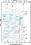 |
Fig. A.1. Spectral time series of SN 2023ixf spanning days 3 to 324. Observations conducted with different instruments are color coded and distinguished by the legend at the top. Phases are marked on the right. Some major telluric lines are identified by ⊕. Some noisy spectra are binned; the original version is plotted with a fainter color. |
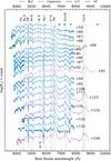 |
Fig. A.1. Continued. |
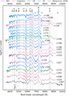 |
Fig. A.1. Continued. |
Appendix B: Fitting [O I] + Hα with multiple Gaussians
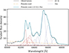 |
Fig. B.1. [O I] + Hα profile of SN 2023ixf at day 298. The observed spectrum (solid black line) is approximated by the dashed light blue line, which consists of a pseudo-continuum (dot-dashed orange line), five Gaussian components of [O I] (solid red lines), and five Gaussian components of Hα (solid dark blue lines). |
All Tables
All Figures
|
Fig. 1. Optical and NIR light curves of SN 2023ixf. Open circles mark the early g-, V-, and r-band light curves from Li et al. (2024). The dashed black line represents the decline expected for 56Co decay. |
| In the text | |
|
Fig. 2. Absolute V-band light curve of SN 2023ixf compared to those of the Type IIP/IIL SNe 1999em (Leonard et al. 2002), 2017gmr (Andrews et al. 2019), 2013ej (Huang et al. 2015), 2006ai (Anderson et al. 2014), 1980K (Buta 1982), and 1990K (Cappellaro & Danziger 1995). All magnitudes have been corrected for the host and the Galactic extinction components. |
| In the text | |
|
Fig. 3. Pseudo-bolometric light curves of SN 2023ixf established with photometry in different wavebands and only the V band. Comparisons with SN 2013ej (Yuan et al. 2016), SN 2006ai (Hiramatsu et al. 2021), and SN 1999em (Valenti et al. 2016) are also included. |
| In the text | |
|
Fig. 4. Spectra of SN 2023ixf at days ∼5 (a), 40 (b), 150 (c), and 330 (d) compared to that of the Type IIP/L SNe 2013ej (Valenti et al. 2014; Yuan et al. 2016; Huang et al. 2015), 1999em (Leonard et al. 2002), 2017gmr (the spectrum at day 312 is binned; Andrews et al. 2019), and 2006ai (Hiramatsu et al. 2021) at similar phases. In each panel, major spectral features are marked by vertical dashed lines. For a better display, all spectra were shifted arbitrarily and presented in a logarithmic scale. |
| In the text | |
|
Fig. 5. pEW of Fe IIλ5018 in SN 2023ixf compared with the models presented by Dessart et al. (2014). The 0.4, 1, and 2 × Z⊙ models are shown by the color-coded lines (see the legend). |
| In the text | |
|
Fig. 6. Comparison of the evolution of the Fe IIλ5169 velocity of SN 2023ixf with those of SNe 2013ej, 1999em, 2005cs, and 2006ai. |
| In the text | |
|
Fig. 7. Temporal evolution of the Hα profile from days 93 to 298. The vertical dashed black lines mark the rest-frame velocities of −2000, −1000, 0, +1000, and +2000 km s−1. |
| In the text | |
|
Fig. 8. Temporal evolution of the spectral line profiles centered at the rest-frame wavelengths of Na Iλ5890, 5896, [O I] λ6300, [O I] λ6364, Hα, [Ca II] λ7291, and [Ca II] λ7323, as labeled in each subpanel. All spectra are presented in velocity space. Three vertical dashed black lines mark the rest-frame velocities of −1500, 0, and +1500 km s−1. The dotted blue lines mark the [N II] λλ6548, 6583 and [S II] λλ6716, 6731 emission lines from an H II region in the host galaxy. |
| In the text | |
|
Fig. 9. NIR spectra of SN 2023ixf observed by TNG from t ≈ 4 to 80 days after the explosion. Phases are indicated to the right of each spectrum. Several prominent spectral lines are marked with vertical dashed lines. Telluric lines are shown with crossed circles and gray shading. |
| In the text | |
|
Fig. 10. Comparison of the NIR spectra of SN 2023ixf with those of SN 2013ej at similar phases. Several prominent spectral features are marked by dashed lines, and telluric absorption is shown with crossed circles and gray shading. |
| In the text | |
|
Fig. 11. Comparison of the nebular-phase spectrum of SN 2023ixf obtained at day 275 and the non-LTE model spectra at day 250 for CCSNe with ZAMS masses of 12, 15, and 19 M⊙. The subpanels in the lower row zoom in on the [O I] + Hα, [Ca II], and Ca II NIR triplet regions. |
| In the text | |
|
Fig. 12. Temporal evolution of the measured [O I] λλ6300, 6364 flux for SN 2023ixf as a percentage of the total optical flux, along with that of the modeled spectra presented by Jerkstrand et al. (2014). |
| In the text | |
|
Fig. A.1. Spectral time series of SN 2023ixf spanning days 3 to 324. Observations conducted with different instruments are color coded and distinguished by the legend at the top. Phases are marked on the right. Some major telluric lines are identified by ⊕. Some noisy spectra are binned; the original version is plotted with a fainter color. |
| In the text | |
|
Fig. A.1. Continued. |
| In the text | |
|
Fig. A.1. Continued. |
| In the text | |
|
Fig. B.1. [O I] + Hα profile of SN 2023ixf at day 298. The observed spectrum (solid black line) is approximated by the dashed light blue line, which consists of a pseudo-continuum (dot-dashed orange line), five Gaussian components of [O I] (solid red lines), and five Gaussian components of Hα (solid dark blue lines). |
| In the text | |
Current usage metrics show cumulative count of Article Views (full-text article views including HTML views, PDF and ePub downloads, according to the available data) and Abstracts Views on Vision4Press platform.
Data correspond to usage on the plateform after 2015. The current usage metrics is available 48-96 hours after online publication and is updated daily on week days.
Initial download of the metrics may take a while.