| Issue |
A&A
Volume 703, November 2025
|
|
|---|---|---|
| Article Number | A169 | |
| Number of page(s) | 14 | |
| Section | Planets, planetary systems, and small bodies | |
| DOI | https://doi.org/10.1051/0004-6361/202555041 | |
| Published online | 13 November 2025 | |
New migration patterns in high planet–star mass ratio systems in discs with low viscosity
1
Leiden Observatory, Leiden University,
PO Box 9513,
2300 RA
Leiden,
The Netherlands
2
Delft University of Technology,
Postbus 5,
2600 AA
Delft,
The Netherlands
3
Facultad de Ingeniería y Ciencias, Universidad Adolfo Ibáñez,
Av. Diagonal las Torres 2640,
Peñalolén,
Chile
4
Instituto de Astrofísica, Pontificia Universidad Católica de Chile,
Av. Vicuña Mackenna 4860,
7820436
Macul,
Santiago,
Chile
★ Corresponding author: This email address is being protected from spambots. You need JavaScript enabled to view it.
Received:
4
April
2025
Accepted:
16
September
2025
Abstract
Context. The migration of giant planets remains a complex and rich topic. While significant progress has been made in understanding migration in discs with high viscosity, the migration of planets with high planet-star mass ratios in low-viscosity environments is still not fully understood.
Aims. Our aim is to study the migration of planets with high planet-to-star mass ratios embedded in low-viscosity protoplanetary discs, characterised by the viscous parameter α = 10−4, and to derive analytical prescriptions that could be used to study planet formation across a range of stellar masses, spanning from Sun-like stars to M dwarfs.
Methods. We performed hydrodynamical simulations using the FARGO3D code, exploring the migration of planets with high planet-star mass ratios (10−3 ≤ q ≤ 2 × 10⁻²) under different disc conditions, including variations in gas surface density, scale height, and density slope.
Results. Our simulations reveal a change in the migration direction at a mass ratio of q ≈ 0.002, with planets exhibiting outward migration for q > 0.002. Additionally, for planets undergoing outward migration, we find that the migration speed depends on the unperturbed local gas density. In most cases, outward migration is driven by a positive torque related to the fact that the planet’s eccentricity remains below e < 0.2. However, under certain disc parameterisations, planets with q > 0.01 can develop higher eccentricities in the range 0.2 < e < 0.45, which can lead to stalled migration.
Conclusions. Our findings suggest that outward migration is a viable mechanism for massive planets in low-viscosity discs, which has implications for the formation and distribution of super-Jupiter planets around Sun-like stars and planets more massive than Neptune around very low mass stars. Given the challenges in detecting such planets, improving our theoretical understanding of their migration is essential for interpreting exoplanet demographics and guiding future observational efforts.
Key words: planet–disk interactions
© The Authors 2025
 Open Access article, published by EDP Sciences, under the terms of the Creative Commons Attribution License (https://creativecommons.org/licenses/by/4.0), which permits unrestricted use, distribution, and reproduction in any medium, provided the original work is properly cited.
This article is published in open access under the Subscribe to Open model. This email address is being protected from spambots. You need JavaScript enabled to view it. to support open access publication.
1 Introduction
Planetary migration, driven by the interactions between planetary embryos and the protoplanetary disc in which they are embedded, is thought to play a crucial role in shaping the architectures of planetary systems. The migration speed and direction of planets depend on both the planet–star mass ratio and the disc’s physical properties. For low-mass planets (or small planet–star mass ratios), migration is typically described by the viscous type I regime (Ward 1997; Tanaka et al. 2002; McNally et al. 2019). This process has been extensively studied, particularly in the context of non-isothermal discs (Paardekooper et al. 2010, 2011; Ziampras et al. 2024b, a, 2025).
When a planet becomes massive enough to carve a gap in the disc, migration transitions to the so-called type II regime (e.g. Lin & Papaloizou 1979). In the classical type II migration model, the torques are strong enough to change the density structure of the disc, and the planet opens a deep annular gap around its orbit. However, hydrodynamical simulations have shown that gas can still drift through the gap (e.g. Masset & Snellgrove 2001), challenging the traditional view of no gas flow across it (e.g. Ward 1997). Moreover, this gap-crossing flow allows massive planets to migrate independently of disc accretion (e.g. Duffell et al. 2014; Dürmann & Kley 2015a). Furthermore, it has been shown that the gap-opening process is influenced not only by the planet’s mass, but also by the disc’s viscosity and scale height (see Crida et al. 2006; Duffell & MacFadyen 2013; Kanagawa et al. 2015). For instance, in a low-viscosity disc (e.g. α = 10−4, where α is a dimensionless measure of the turbulent viscosity in protoplanetary discs), even a Neptune-mass planet can create a gap.
An improved analytical framework to describe the gas structure around gap-opening planets was proposed by Kanagawa et al. (2017). They showed that a planet interacts mainly with the gas at the bottom of the gap, which is consistent with the results obtained by hydrodynamic simulations. Building on this approach, Kanagawa et al. (2018) created a model for type II migration that is basically type I but reduced due to the lower density inside the gap. They studied the migration of planets with planet–star mass ratios (denoted by q) less than 10−3 and gas viscosities described by the parameter α = 10−2 and α = 10−3. On the other hand, Robert et al. (2018) studied the migration of an accreting planet until it reaches the mass of Jupiter, considering lower viscosity values 3 × 10⁻⁴ < α < 3 × 10⁻³. They concluded that what drives type II migration is the imbalance between the torques felt by the planet from the inner and outer discs, as pointed out by Dürmann & Kley (2015a). Moreover, they found that gap-crossing flows are actually negligible at low viscosity, and that cutting this small gas flow with planetary accretion hardly impacts the migration speed.
Additional investigation has been conducted for planets that are more massive than the local disc’s mass, and it has shown that their migration not only slows down (Syer & Clarke 1995; Ivanov et al. 1999), but can also reverse direction (Crida et al. 2007; Hallam & Paardekooper 2018). In a recent study, Dempsey et al. (2021) investigated the migration of planets in fixed orbits within the mass range 10−3 < q < 2 × 10⁻², considering viscosity parameters between 10−3 < α < 10−1. Their results revealed cases of positive torques, which were linked to non-negligible disc eccentricities. Building on this, Scardoni et al. (2022) extended the analysis by allowing the planets to change their orbits, and examined the resulting torques. They identified a correlation between migration speed and the parameter K, as well as a threshold distinguishing inward from outward migration. Additionally, they emphasised the role of planetary orbital eccentricity in determining the migration direction. Although these studies are based on viscous disc evolution, recent proposals involving wind-driven disc evolution suggest that outward migration may still be possible for massive planets (Kimmig et al. 2020).
Most previous studies have assumed high gas disc viscosity values (α > 10−3). However, recent ALMA observations suggest that turbulence within protoplanetary discs is weak, corresponding to α < 10−4 (e.g. Flaherty et al. 2018, 2020; Villenave et al. 2020, 2022; Pizzati et al. 2023). Additionally, low viscosities may provide a better explanation for certain observed features in protoplanetary discs (see Rosotti 2023). For instance, in low-viscosity discs, a single planet can create multiple gaps (Bae et al. 2017; Dong et al. 2017, 2018), even while migrating (e.g. Weber et al. 2019). Moreover, high-viscosity values lead to the formation of large protoplanetary discs extending hundreds of astronomical units, which have not been observed (Toci et al. 2021). Additionally, compact discs only a few astronomical units in size appear to be the most common around low-mass stars (M★ < 1 M⊙) (Guerra-Alvarado et al. 2025). Therefore, understanding planet formation around low-mass stars requires a planet migration recipe valid for high-mass planets in low-viscosity discs.
Although giant planets are significantly less common around M dwarfs than around Sun-like stars, consistent with expectations from the core accretion model (e.g. Laughlin et al. 2004), the number of confirmed giant planets orbiting M dwarfs has been steadily increasing. Their occurrence rate is less than 1 % (e.g. Bonfils et al. 2013; Sabotta et al. 2021), and so far it has been challenging to reproduce with current planet formation models (e.g. Emsenhuber et al. 2021). In particular, their formation becomes difficult when the available dust reservoir is limited to a few Earth masses (Sanchez et al. 2024). Recently, Stefánsson et al. (2023) showed that a Neptune-like planet with an orbital period of just a few days can be formed around a 0.1 M⊙ star, given an initial dust reservoir of 50 M⊕. Similarly, Pan et al. (2024) demonstrated that giant planets with masses up to that of Saturn may form within 100-day orbits in high-viscosity discs (α > 10−3), provided the dust reservoir exceeds 50 M⊕. Nonetheless, further studies are needed to fully understand their formation as well as migration across different regions of the disc, and to reproduce their occurrence rate.
Planet formation models around low-mass stars are hampered by the lack of reliable migration prescriptions for high planet–star mass ratios in low-viscosity discs. Therefore, in this work we explore planetary masses and low-viscosity discs, which are relevant around low-mass stars. We performed hydro-dynamical simulations of high planet–star mass ratios (10−3 ≤ q ≤ 2 × 10⁻²) in low-viscosity discs (α = 10−4) and explored a wide range of disc physical parameters. We note that while such planet–star mass ratios correspond to Jupiter-like up to super-Jupiter-like planets around Sun-like stars, they represent planets with masses between 20 M⊕ and 2 Jupiter masses around low-mass stars of 0.1 M⊙.
This work is structured as follows. In Section 2, we describe the setup of the hydrodynamical simulations and the proposed scenarios of study. In Section 3, we present the simulation outcomes, including estimates of total torques and the evolution of planetary orbits. We also provide prescriptions for the migration of massive planets in low-viscosity discs and calculate the migration timescales to compare them with exoplanet occurrence rates. In Section 4, we discuss the limitations of the model and potential future improvements. Finally, in Section 5, we summarise our work and highlight key findings.
2 Method
To calculate the planet–disc interactions of a single planet embedded in a gas-disc, we used FARGO3D1 (Benítez-Llambay & Masset 2016). We set the code to solve the equations of hydrodynamics in two dimensions on an Eulerian polar mesh. Similar to its predecessor (FARGO; Masset 2000), the code incorporates fast orbital advection algorithms, thus allowing for the study of planet–disc interactions over long periods of time. It has been widely used in this field and has demonstrated strong performance across the full range of planetary masses. In particular, it effectively handles the interactions of giant planets, which carve gaps in the disc and generate strong shocks in their surrounding (e.g. de Val-Borro et al. 2006).
2.1 Setup
We follow the setup from Kanagawa et al. (2018) (hereafter K18). Therefore, the radius unit was determined by the initial location of the planet, r0, and the mass unit was determined by the stellar mass, M★. Thus, the surface density unit is  . We modelled the initial disc surface density, Σ(r), with a power law,
 (1)
(1)
where Σ0 is the gas-disc density at r = r0, with r as the radial distance to the star. Similarly, we assumed a power law for the disc aspect ratio,
 (2)
(2)
where h0 is the disc aspect ratio at r = r0. We assumed a steady viscous accretion disc where the factor Σν is constant, with the disc viscosity as ν = αcsH, cs = ΩkH as the sound speed, Ωk as the Keplerian frequency, and H = hr as the scale height of the disc (Shakura & Sunyaev 1973). Following the approach of K18, the density index, s, was connected to the flaring index, f, by the relation s = 2f + 0.5.
We set α = 10−4 and did not explore lower values, as for low-viscosity discs with α < 10−4 vortices from the Rossby Wave instability may alter the planet’s orbit, causing eccentricity growth and erratic inward migration (e.g. McNally et al. 2019). This erratic migration would be hard to capture in a simple torque prescription.
We divided the grid into 128 cells in the radial direction (equally spaced in logarithmic space) and into 512 cells in the azimuthal direction (equally spaced). Thus, one grid cell corresponds to approximately 0.4H for H/r = 0.05. We note that our resolution is lower than that used in Kanagawa et al. (2018), as adopting a lower viscosity significantly increases the computational cost at higher resolutions. We applied damping in the wave-killing zones of the disc to avoid artificial wave reflection following de Val-Borro et al. (2006). The wave-killing zones have a width approximately equal to 10% of the radius of the mesh edges, defined as rin = 0.4r0 and rout = 3r0, respectively, for the inner and outer edge of the disc. Consequently, the quantity Δr/r = 0.015 and Δθ = 0.012. Therefore, the number of cells spanning the horseshoe region ranges from 10 to 26 in the radial direction, for mass ratios 10−3 < q < 2 × 10⁻².
In order to define the gravitational potential of the planet, we used the softening parameter ϵ = 0.6H0. We included the indirect term of the planet, and we modified the code to exclude 60% of the Hill radius of the planet when calculating the force exerted by the disc onto the planet, accounting for the presence of a cir-cumplanetary disc, following Crida et al. (2009). For simplicity, we neglected the accretion of disc gas onto the planet (see Section 4 for discussion on this choice). The planet is allowed to migrate through the disc.
The main difference with K18 is that we considered higher mass ratios, 10−3 < q < 2 × 10⁻². These correspond to planetary masses between 1 and 20 Jupiter masses for a Sun-like star, and between 20 M⊕ and 2 Jupiter masses for a star of 0.1 M⊙.
2.2 Cases of study
The parameter K that describes the gap depth is associated with the planet–star mass ratio, q, aspect ratio, h, and viscosity parameter, α, by:
 (3)
(3)
First, we aim to explore the same range in K-parameter studied by K18, but for migrating planets that do not follow type I migration, associated with 100 < K < 104 and embedded in a low-viscosity disc (α = 10−4). Following the fiducial case in their study, we set Σ0 = 10−4, h0 = 0.05 and s = 0.5. The cases studied to recover the same value of K as K18 with our lower value of α, are associated with the following planet–star mass ratios q: 1 × 10⁻⁵, 5 × 10⁻⁵, 1 × 10⁻⁴, 5 × 10⁻⁴, and 1 × 10⁻³.
Motivated by the fact that, for a very low-mass star of 0.1 M⊙, the highest value of K explored by K18 (considering α = 10−4 and h0 = 0.05) corresponds to a planet with a mass of only 20 M⊕, we extended the study to higher K values. This expansion allows us to explore the dynamics of more massive planets orbiting very low-mass stars. Thus, we expanded our study to K = 2 × 10⁷ which corresponds to a planet with 2 Jupiter-mass around a low-mass star of 0.1 M⊙.
In this new K domain, we explored six different values of planet–star mass ratios 5 × 10⁻⁴, 1 × 10⁻³, 3 × 10⁻³, 5 × 10⁻³, 1 × 10⁻², and 2 × 10⁻². Additionally, we varied several discs parameters, including 0.03 < h0 < 0.07, 0.5 < s < 1, 10−6 < Σ0 < 10−3, and 10−4 < α < 10−2. The cases of study are listed in Table 1. We note that the planet was inserted at t = 0 with its final mass, without employing a growth function to gradually increase the planetary mass over time (e.g., Griveaud et al. 2023). As a result, the disc undergoes an impulsive perturbation at the beginning of the simulation rather than a gradual adjustment to the planet’s presence. However, these initial transients dissipate relatively quickly and do not affect the long-term torque evolution or migration trends.
In total, 64 simulations were performed during 40 000t0, with t0 the orbital period at r = r0. We note that the simulations needed to be run for an extended period because the viscous timescale of the disc, which determines how quickly the disc reacts to the planet’s presence, is typically much longer in low-viscosity discs. As a result, a longer simulation duration is necessary for the disc to adjust and for a stable interaction between the planet and the disc to be reached. We also point out that in the simulations, the planet migrates only a short distance from its initial location (less than ~5%). As it remains close to its starting point, even in the case of f ≠ 0, the value of h stays approximately constant, and so does the corresponding value of K.
Set of parameters that changed in the simulations.
3 Results
We detail the procedure used to estimate the torques exerted by the gas disc on the planet, based on the outcomes of our hydro-dynamical simulations. Additionally, we present the resulting torques for the different cases of study proposed in the previous section. Furthermore, we introduce new prescriptions to account for the expanded parameter space explored in this work. Finally, we estimate migration timescales and compare them with occurrence rates of giant planets.
3.1 Quantifying torques and planetary dynamics
In order to determine the torque that the gas-disc exerted onto the planet, we integrated our simulations for around 40 000 orbits. Even for these long integration times, the low-viscosity (α = 10−4) nature of the disc means that true steady states are hard to reach. For quantifying the torques, we employed a Savitzky–Golay filtering that applies a polynomial smoothing technique to the data, which smooths data while preserving features such as peak height, width, and slope better than a running average (Savitzky & Golay 1964).
As an example, in Figure 1 we show, for a mass ratio q = 3 × 10⁻³, the evolution of the torque measured in the simulation Γ normalised to the scaling torque Γ0, which is defined by:
 (4)
(4)
We also include the corresponding smoothed fitting function obtained from the torque data to show the trend in the torque evolution. We can see that the torque changes sign after approximately 15000 orbits, becoming positive and approaching the value Γ/Γ0 ≈ 0.0006. Although the torque did not reach a steady state within the integration period, it appears unlikely that the torque will undergo any qualitative changes.
Additionally, we analyse the distributions of the azimuthally averaged gas surface density, normalised by the initial unperturbed local density of the planet, alongside the evolution of the semi-major axis and eccentricity of the planet throughout the integration. As an example, Figure 1 also illustrates these three quantities for the case of q = 3 × 10⁻³. It shows that the position of the gap carved by the planet in the density profile shifts according to the torque’s sign, moving either inwards towards the star or outwards. Furthermore, since the eccentricity remains small (e < 0.015), the negative torque corresponds to inward migration, as indicated by the decreasing semi-major axis over time. Once the torque becomes positive, the planet reverses direction and begins to migrate outward.
We present the normalised torques from simulations with low viscosity (α = 10−4) and standard values Σ0 = 10−4, h0 = 0.05, and s = 0.5 in Figure 2. The torques are categorised as negative, positive, or those remaining close to zero. For the same K interval explored by K18 (100 < K < 104), our results show good agreement, with the torque values aligning well with their fitting function:
 (5)
(5)
with the fitting constant c = 3. In principle, it seems like the fitting function could be applied up to K = 4 × 10⁴. Beyond this value, there is a narrow range where migration may halt (represented in this case by q = 0.0015), and for K between 105 and 106, we observe positive torques consistent with outward migration. For the highest K values (up to K = 2 × 10⁷), associated with q = 0.01 and q = 0.02, we found either slight outward migration or negligible migration. When the torques are positive and the planet is migrating outwards, the eccentricity remains close to zero. However, for the highest mass ratios considered, we observe that the planet’s eccentricity can reach values in the range 0.2 < e < 0.45. In particular, for the case of q = 0.01, we observe a negative torque associated with outward migration and a growing eccentricity up to around 40 000 orbits. To better characterise the migration path, we extended the simulation by an additional 20 000 orbits. We found that the planet’s eccentricity peaks at approximately e ~ 0.3, followed by small oscillations. These oscillations are also reflected in the evolution of the semi-major axis, which gradually decreases until both parameters eventually stabilise over time. These results confirm that planets with high mass ratios, q, can experience eccentricity growth up to about 0.45, while remaining gravitationally bound to their host star. The evolution of the semi-major axis and eccentricity for the cases of outward or negligible migration is illustrated in Figure 2.
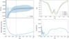 |
Fig. 1 Top panels: evolution of the normalised torque, along with the smoothing function, over the integration (left) for a planet with q = 0.003 in a low-viscosity disc (α = 10−4) with Σ0 = 10−4, and h = 0.05. Distribution of the azimuthally averaged gas-disc density around the planet’s initial location at three different integration times (right). Bottom panels: evolution of the semi-major axis (left) and eccentricity (right) of the planet during the integration. The vertical lines mark the times when the torque changes sign, indicating a reversal in the direction of the planet’s migration. Time is expressed in units of t0, the orbital period of the planet at r = r0. |
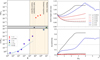 |
Fig. 2 Left: normalised positives (red dots), negatives (blue and pink for q ≤ 1 × 10⁻³), and close to zero (black) torques as a function of a wide range of the K-parameter, including the previously studied domain by K18 (white background) and the new domain explored in this work (cream background), assuming α = 10−4, h0 = 0.05, s = 0.5, and Σ0 = 10−4. The fitting proposed by K18 in the K-range of their study (solid blue line) together with the potential extension in the new regime (dotted blue line) is given in Eq. (5). Torques exerted onto planets in orbits with e > 0.2 are highlighted (green circles). Four different migration regimes are marked indicating inward migration, a halt in migration, outward migration, and migration stalls (dotted grey lines). Right: evolution of the semi-major axis (top) and the eccentricity of the six planets that experience either outward migration or a halt in migration: q = 1.5 × 10⁻³ (dotted black line), q = 2 × 10⁻³ (dashed-dotted red line), q = 3 × 10⁻³ (dashed red line), q = 5 × 10⁻³ (solid red line), q = 1 × 10⁻² (solid blue line), and q = 2 × 10⁻² (solid black line). The value of eccentricity e = 0.2 that gives the change in the torques sign is overplotted (grey dotted line). The simulation for the planet with q = 0.01 was extended to allow eccentricity to settle. |
3.2 Measured torques and their dependence with K
To gain deeper insight into migration trends at high K values for mass ratios 5 × 10⁻⁴ ≤ q ≤ 2 × 10⁻², we analysed torque values under a range of disc conditions, as summarised in Table 1. Figure 3 presents the normalised torques obtained for different combinations of h0, s, Σ0, and α.
As shown in Figure 3, for local surface densities Σ0 > 10−5, the normalised positive torque values are scattered within the same order of magnitude across the explored range of h0. Additionally, we found qualitatively similar results when varying the density slope from s = 0.5 to s = 1 (h0 = 0.05). In the cases explored in this work, the planets exhibit slow migration timescales. However, we acknowledge that, as shown by Paardekooper et al. (2010, 2011), the total torque – particularly the corotation component – can strongly depend on the local density slope, independently of the planet’s orbital evolution. The weak dependence observed in our simulations likely reflects the fact that the corotation torque is strongly diminished in the gap-opening regime, causing the total torque to become less sensitive to the local surface density slope.
In contrast, for a lower surface density Σ0 = 10−5, the normalised torque strength increases. However, examining the non-normalised torques reveals that their absolute values decrease with decreasing local disc density, consistent with slower migration rates as expected from Baruteau et al. (2014). Additional simulations with Σ0 = 10−6 and Σ0 = 10−7 produced normalised torque values nearly identical to those obtained with Σ0 = 10−5, reinforcing this trend. These cases are not shown in Figure 3 to avoid over-plotting, as the resulting values would be indistinguishable from those already displayed.
We note that, for cases with Σ0 ≥ 10−4 and h0 < 0.05, planets with mass ratios q = 0.01 or q = 0.02 tend to reach eccentricities in the range 0.2 < e < 0.45, while the absolute torque values remain negative or close to zero. In particular, after 40 000 orbits, planets with q = 0.01 which exhibit negative torques during the phase of eccentricity growth, are expected to stop migrating once the eccentricity stabilises (see Section 3.1). These results highlight the significant influence of planetary eccentricity on migration behaviour. Notably, even when torques are negative, outward migration can still occur if the planet follows an eccentric orbit, as it is the total work done by the disc that ultimately determines the migration direction (Cresswell et al. 2007; Benítez-Llambay 2024). Further analysis of the 2D gas density map reveals a pronounced asymmetry in the gap carved by the planet, indicating a growing eccentricity in the disc itself. This disc eccentricity may contribute to the evolution of the planet’s eccentricity. These findings are consistent with previous studies (Papaloizou et al. 2001; Goldreich & Sari 2003; Kley & Dirksen 2006), showing that eccentricity growth is favoured in discs with low aspect ratios and low viscosities, particularly for gap-opening planets.
On the other hand, when exploring higher values of α while keeping Σ0 = 10−4, h0 = 0.05, and s = 0.5, we measured positive torques for all planets with q < 0.01, consistent with results reported by Dempsey et al. (2021). However, for the highest mass ratio considered in this study (q = 0.02), the torques remain negative. When the eccentricity stays below e < 0.2, positive torques are related to outward migration, while negative torques corresponded to inward migration. We also observe that, within the explored K range, higher viscosities introduce greater scatter in the absolute torque values, and the direction of migration becomes less stable at the highest mass ratios. In contrast, for low viscosities, outward migration persists up to the largest mass ratios considered, although it may slow or stall rather than reverse direction.
Overall, across all our simulations assuming a low-viscosity disc, we do not find a straightforward relation between the strength of the torque and the K-parameter. Interestingly, we observe a halt in migration that marks a transition in migration direction, associated with a mass-ratio q ≈ 0.002, depending on the physical properties of the disc. This is explored in more detail in the following section.
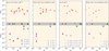 |
Fig. 3 Normalised torques vs the K-parameter range proposed in this study for the mass ratio 5 × 10⁻⁴ < q < 2 × 10⁻² a) with fixed α = 10−4 and Σ0 = 10−4, varying h0 or s; b) with fixed α = 10−4, h0 = 0.05, and s = 0.5, varying Σ0; c) by changing h0, s and Σ0 to simulate realistic conditions along the disc; d) with fixed Σ0 = 10−4, h0 = 0.05, and s = 0.5, varying α. Same colour palette as in Figure 1. |
3.3 Migration reversal at mass-ratio q ≈ 0.002
To reinforce the robustness of the migration direction change at q ≈ 0.002 and its independence from the K-parameter, we ran additional simulations with planets with q = 0.002 embedded in low-viscosity discs (α = 10−4), characterised by aspect ratios h0 from 0.03 to 0.2, covering a wide range of K values from 102 to 107. As a result, as long as K > 104, we consistently find that planetary migration either stalls or becomes slightly outward at q = 0.002. However, for K < 104 we recover inward migration as in K18.
We realised that at a mass ratio q = 0.002, migration behaviour is highly sensitive to the disc’s physical properties. For h0 = 0.05, the torque becomes positive, indicating outward migration, while for h0 = 0.03 and h0 = 0.07, the torque is nearly zero at the same mass ratio, assuming a surface density slope s = 0.5. However, when the surface density slope steepens to s = 1, in the case of h0 = 0.05, the simulation shows migration stalls at this mass ratio (not at q = 0.0015 as in the default scenario with s = 0.5). This sensitivity indicates that planets with mass-ratios, q, between 0.0015 and 0.002 reside in a nonlinear migration regime where small variations in disc structure—such as scale height and surface density slope- can significantly alter the torque balance by affecting Lindblad and corotation torques. This highlights the complexity of migration in low-viscosity discs, where small structural changes can have outsized impacts on the migration direction and rate.
This led to the emergence of a robust and consistent pattern:
Planets with q < 1.5 × 10⁻³ for K > 104 consistently experience inward migration.
Planets with q between 0.0015 and 0.002 can experience a halt in migration, depending on the disc’s physical properties.
Planets with 2 × 10⁻³ < q < 2 × 10⁻² for K < 2 × 10⁷ undergo outward migration, provided their eccentricities remain below e < 0.2.
This transition in migration direction is illustrated in Figure 4, which compiles all normalised torques estimated for planets in low-viscosity discs with e < 0.2.
Furthermore, for planets undergoing outward migration in low-viscosity discs (α = 10−4) with e < 0.2, we found that the torque strength correlates with the local gas surface density according to the following relation:
 (6)
(6)
with a = 5 × 10⁻⁴ and b = 10−5. These fits are shown in Figure 5, along with the measured normalised positive torques driving outward migration for planets with 2 × 10⁻³ < q < 2 × 10⁻².
Notably, for each fitting prescription, all measured torques fall within two standard deviations of the logarithmic residuals (σ = 0.44 dex and σ = 0.32 dex, respectively), demonstrating how well the fit reflects the torques estimated from the simulations.
To avoid a discontinuity at Σ0 = 10−5, we further propose the following function:
 (7)
(7)
where ffit = 1/(1 + (Σ0/10−5)5) is a smooth transition function designed to preserve the same torque values as for Σ0 = 10−5 in the low-density regime (Σ0 < 10−5). Figure 6 shows the application of this function to estimate normalised torques across the range of mass ratios and local gas densities studied in this work. We note that for the intermediate mass ratios q ~ 0.003–0.005, lower disc surface densities lead to stronger (more positive) normalised torques due to enhanced gap asymmetry. At higher mass ratios q > 0.005, the planet dominates the local dynamics,ing the torque less sensitive to the disc mass. This explains the convergence of normalised torques at high q across different disc densities.
These results offer a consistent framework to interpret outward migration trends in low-viscosity discs. They also have potential applications in population synthesis and planet formation models.
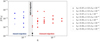 |
Fig. 4 Normalised torques for the different mass ratios associated with planets in low-viscosity discs (α = 10−4) and with orbital eccentricities e < 0.2. The transition between inward (blue symbols) and outward (red symbols) migration (shaded area) occurs for q between 0.0015 and 0.002 (black dots), depending on the disc’s physical parameters. Symbols and colours are the same as in Figure 3. For cases with near-zero torque, values around 1 × 10⁻⁵ were used for better visibility in the figure. |
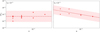 |
Fig. 5 Absolute values of the normalised torques for planets undergoing outward migration in low-viscosity discs (α = 10−4) with 2 × 10⁻³ < q < 2 × 10⁻² and e < 0.2 (see Table 1). Left: results from the simulations assuming a local density Σ0 > 10−5. Right: results from the simulations assuming Σ0 < 10−5. In each panel, the fitting function proposed in this work (dashed red lines-see Eq. (6)) along with a region within ±2 the standard deviation of the logarithmic residuals (red shadow area). Symbols and colours are as in Figure 3. |
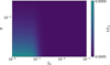 |
Fig. 6 Normalised torque map for the different values of mass ratios (q) and localdensities (Σ0) explored in this workforplanets in low-viscosity disc (α = 10−4) with eccentricity values e < 0.2. |
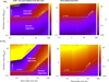 |
Fig. 7 Maps of semi-major axis evolution timescale for different planetary masses and semi-major axis for a 1 M⊙ star (top) and for a 0.1 M⊙ star (bottom), assuming a low-viscosity disc (α = 10−4) with gas surface density and aspect ratio profiles described in Eqs. (1) and (2), assuming s = 0.5 (f = 0) in the inner disc and s = 1 (f = 0.25) in the outer disc. The transition was set at rtrans = 0.3 au for M★ = 0.1 M⊙, and at rtrans = 2 au for M★ = 1 M⊙. We assumed r0 = rtran, and characterised both the inner and outer disc by Σ0 = 4 × 10⁻⁴ M⊙/au2 and h0 = 0.03, simulating the conditions of a disc at 1–2 Myr with a high gas disc mass ~10% M★. Limits for inward and outward migration are overplotted (dashed grey lines). Right: timescales calculated applying only the fitting function from K18 (see Eq. (5)). Left: timescales calculated combining the fitting function from K18 for K < 104 and q < 0.002, and the fitting functions propose in this work (see Eq. (6)), for 0.002 < q < 0.02 and K < 2 × 10⁷, relating the surface density Σ(r) to Σ0 = 10−5 M★/r2 (dotted grey line). |
3.4 Estimation of migration timescales across the disc
We aim to quantify migration for planets with different masses, within the range considered in this study, embedded in a low-viscosity disc (α = 10−4). Since our analysis focuses on planets in nearly circular and coplanar orbits, the migration timescale, defined as the rate of change in angular momentum, can be expressed as τm ≈ 2τα, where τα denotes the timescale associated with the change in semi-major axis:
 (8)
(8)
Therefore, we computed τα for giant planets throughout the disc, following the normalised torque fitting function proposed by K18 (see Eq. (5)) for planets migrating inwards, and the fitting function introduced in this work (see Eq. (7)) for planets migrating outwards. We computed the scaling torque using the gas surface density and aspect ratio profiles described in Eqs. (1) and (2), assuming s = 0.5 (f = 0) in the inner disc to simulate a viscous disc, and s = 1 (f = 0.25) in the outer disc to represent an irradiated disc (e.g., Ida et al. 2016). We assumed r0 = rtran, the transition radius between the inner and outer disc. For a star of M★ = 0.1 M⊙, this transition is set at rtran = 0.3 au, while for M★ = 1M⊙ it is set at rtran = 2 au. In both cases, we adopted inner and outer disc profiles characterised by Σ0 = 4 × 10⁻⁴ M⊙/au2 and h0 = 0.03, simulating the conditions of a disc at 1–2 Myr with a high gas disc mass ~10% M★.
Figure 7 presents maps of the absolute value of τα across different planetary masses and semi-major axes for stars of 0.1 M⊙ and 1M⊙. For comparison, these maps include the results of applying the new migration patterns introduced in this work, along with those considering only the inward migration model proposed by K18. We note that the disc density will be smaller than 10−5 M★/r2 for large radial distances (r > 100 au), but also for a small region close to the inner edge of the disc. Near the inner edge of the disc, the surface density at the planet’s location typically exceeds 10−3 M⊙/au2. For example, for a M★ =0.1 M⊙ and r = 0.025 au, this corresponds to ~9 × 10⁻⁶ M★/r2 in code units – just below the 10−5 threshold. We also ascribe to the fact that the upper limit for outward migration in our study is defined by the highest K-value examined (K = 2 × 10⁷). As migration appears to slow down with increasing K, we associate the region with Κ > 2 × 10⁷ with slower migration rates. However, this is linked to even higher mass ratios, and a further study, which fall outside the scope of this work, is needed to properly estimate the timescales.
Regardless of the stellar mass, we observe that the new normalised torques estimated in this work allow giant planets to experience different migration speeds and directions. In particular, for planets with masses Mp > 2 Jupiter mass for a star of 1 M⊙, and for planets with masses Mp > 0.2 Jupiter mass for a star of 0.1 M⊙.
These new findings on outward migration in low-viscosity discs provide a new perspective on giant planet formation. They suggest how such planets may form throughout the disc.
3.5 Linking giant planet occurrence rates and migration timescales
Motivated by the varying patterns of migration across the disc, we seek to qualitatively compare the occurrence rates of giant planets with their estimated migration timescales, which are associated with the time it takes for a planet to undergo significant orbital migration due to interactions with the surrounding protoplanetary disc. Specifically, we compared occurrence rates of giant planets with migration timescales for stars of 1 M⊙ and 0.1 Μ⊙, respectively. For FGK stars, we adopt the occurrence rates of planets with masses between 0.1 and 20 Jupiter masses from Fernandes et al. (2019), derived from a log-normal distribution (μ = 3.16 au, σ = 0.75 dex) that fits Kepler data (Bergsten et al. 2022), as well as radial velocity (Fulton et al. 2021) and direct imaging data (Vigan et al. 2017). For M dwarfs, we adopted the occurrence rates of giant planets with masses between 1 and 10 Jupiter masses, by integrating the maximum-likelihood log-normal distribution proposed by Meyer et al. (2018), which compiles results from various observational techniques. To ensure completeness, we also included the estimates from Clanton & Gaudi (2014), which combine constraints from microlensing and radial velocity for planets between 0.1 and 13 Jupiter masses, spanning orbital periods between 100 and 10000 days (corresponding to semi-major axes between 0.2 and 5 au). Additionally, occurrence rates for planets with masses between 0.1 and 1 Jupiter mass around M dwarfs at separations a < 1 au (assuming M★ = 0.1 Μ⊙) have also been reported, and remain low, below 0.16% (Sabotta et al. 2021).
In Figure 8, we present the occurrence rates as a function of semi-major axis for FGK stars and M dwarfs, correlated with the average migration timescale at each location, within the mass range described above, which is associated with the calculation of occurrence rates. We note that planets located at a < 1 au exhibit the fastest migration, consistent with the lowest occurrence rates estimated in previous works. Additionally, there is an increase in migration timescales for planets located between 3 and 10 au, which corresponds with higher occurrence rates. We emphasise that, at least for the inner disc region (in this example, a < 0.3 au around the M dwarf and a < 2 au around the Sun-like star), where the surface density slope is s = 0.5, the migration timescale (τm) is independent of the planet’s orbital distance from the star. Therefore, any variation in migration timescale across the inner disc reflects genuine physical differences in the torque acting on the planet, rather than being a simple consequence of orbital period scaling.
On the other hand, the estimated migration timescales for planets beyond a > 10 au are still high, which contradicts the observed drop in occurrence rates at these locations. One possible explanation for this discrepancy is that migration timescales are typically calculated under the assumption of quasi-circular orbits, whereas most giant planets beyond 10 au exhibit high eccentricities2. Since eccentric orbits lead to faster migration this could help reconcile the lower occurrence rates observed at these distances, considering just the planets with q < 0.02. Another possible explanation is that giant planet formation becomes inefficient beyond 10 au. As suggested in previous studies, core formation timescales increase significantly at larger distances from the star (e.g. Morbidelli & Raymond 2016). Furthermore, if planet formation could take place at such a location, the low migration timescales could keep the planet fixed at wider orbits, and provide an explanation for planet-inferred gaps in protoplanetary discs (e.g. Lodato et al. 2019; van der Marel 2023; Guerra-Alvarado et al. 2025). Overall, the fact that super-Jupiters migrate outwards could explain some of the directly imaged planets in the 10–100 au range (Vigan et al. 2017; Nielsen et al. 2019).
This analysis suggests that the faster migration of planets located around 0.3 au – often referred to as the ‘warm Jupiter desert’ – could be explained by their shorter migration timescales. Meanwhile, the slower migration of planets located between 3 and 10 au, coupled with their higher occurrence rates, highlights the interplay between migration dynamics and observed exoplanet demographics. Moreover, we note that the migration timescales for planets with a > 1 au around M dwarfs are 2–3 times longer than those for planets orbiting FGK stars. This finding provides new insight into giant planet formation around low-mass stars, as slower migration timescales are crucial for their formation. For instance, the Bern planet formation model (Emsenhuber et al. 2021) requires reduced migration rates around low-mass stars to enable giant planet growth.
We also note that close-in planets with semi-major axis a < 0.1 au, commonly referred to as ‘Hot Jupiters’, are associated with low occurrence rates and very short migration timescales. The outward migration pathway identified in this work for planet-to-star mass ratios q > 0.002 effectively rules out the formation of such planets via inward migration. Therefore, their formation is more likely to result from high-eccentricity migration – triggered by planet-planet scattering followed by tidal circularisation (e.g., Rasio & Ford 1996; Ford & Rasio 2008; Nagasawa et al. 2008). Alternatively, in situ formation has been proposed by other authors (e.g., Boley et al. 2016; Batygin et al. 2016). However, this scenario remains challenging, as it would require planet formation to occur late in the disc’s evolution, when outward migration is expected to be negligible.
These insights provide a deeper understanding of the distribution of giant planets. They also point to the mechanisms that could be responsible for shaping their final orbital configurations.
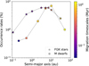 |
Fig. 8 Occurrence rates of giant planets with masses between 0.1 and 20 Jupiter-masses as a function of semi-major axis, correlated with migration timescales at each location, for FGK stars and M dwarfs. Quasi-circular orbits are assumed for the planets. |
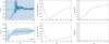 |
Fig. 9 Comparison of the normalised torques (right panels), evolution of the semi-major axis (middle panels), and evolution of the eccentricity (left panels) of the planet from the case of study shown in Figure 1, for two different resolutions: the one used in K18 (top) and the one used in this work (bottom). |
4 Discussion
Our aim was to extend the analysis conducted by K18 to investigate the migration paths of single giant planets embedded in low-viscosity protoplanetary discs. However, due to the computational cost of such simulations, we chose to lower the resolution compared to the one used by K18. Prior to making this adjustment, we replicated several of K18’s simulations to ensure that the normalised torques obtained with the reduced resolution were consistent with their results. As an example, in Figure 9, we show the normalised torques along with the corresponding fitting function, as well as the evolution of the semi-major axis and eccentricity for a planet with q = 3 × 10⁻³, using the same scenario as in Figure 1. Two different resolutions are considered: the one used in this work (see Section 2) and the one proposed by K18, which is four times higher. The results confirm that in both cases, the same value of the normalised torque is achieved. With higher resolution, the planet reaches this value more quickly in its orbital evolution. In both cases, once the torque changes sign and becomes positive, the semi-major axis evolution shows that the planet begins migrating outwards, and eccentricity is e < 0.2. Furthermore, we note that the normalised torque exhibits oscillations over time, which are linked to the planet’s epicyclic motion. In particular, in the high-resolution case, as the planet reaches a higher eccentricity, the epicyclic motion has a larger amplitude, which leads to torque oscillations of greater amplitude.
In FARGO3D, the gas is not self-gravitating and orbits only under the influence of the star’s potential, while an embedded planet experiences a combined stellar and disc potential. This discrepancy shifts the Lindblad and corotation resonances, affecting the planet’s migration velocity, as demonstrated by Baruteau & Masset (2008). A solution to this is to remove the azimuthally averaged density from the density of each zone before evaluating the forces, allowing the planet to feel only the star’s gravity (see e.g., Benítez-Llambay et al. 2016). In order to compare with K18, we did not subtract the asymmetric component of the disc’s gravity from the force on the planet. However, to test the impact of this effect for high planet–star mass ratios, we activate the subtraction of this effect. Our results showed that this leads to smoother evolution of the torques and semi-major axis, and while the differences get larger with increased surface density, qualitatively the results do not change, as for the high mass ratios (0.002 < q < 0.02) planets still migrate outwards at a comparable speed.
We note that following K18, we did not include the disc’s indirect term in our main simulations. While it can be argued that it should be included on physical grounds, we found that it can also lead to artificial growth of eccentricity in the disc, resulting in inaccurate planetary migration behaviour (see Appendix A). Given its potential relevance (e.g., Benítez-Llambay et al. 2016; Crida et al. 2025), we performed test runs to assess its impact on the planet’s dynamical evolution and on the final torque estimates. In these tests, the disc’s indirect term is applied consistently to both the gas and the planet. As a result, for planets with e < 0.2, we found no qualitative differences in the torque measurements during the quasi-steady-state phase, density maps, or migration direction – suggesting that the system behaves similarly whether or not the indirect term is included. In a more extreme case with q = 0.01 and Σ0 = 10−3, including the indirect term introduces a positive torque contribution. Still, migration stalls in both cases, and the planet’s orbit remains stable, indicating that long-term evolution is not significantly affected. An intermediate case with q = 0.01 and Σ0 = 10−4 shows lower eccentricities when the indirect term is included with values e < 0.25. In summary, including the indirect term in the disc has only a modest impact on the overall migration behaviour in the scenarios studied. Although it slightly modifies the early torque evolution and eccentricity damping, the long-term trends, such as migration direction and the final strength of the torques, remain broadly consistent, and within the scatter considered in our analysis (see further details in the Appendix A).
The torques measured in the simulations arise from the gas perturbations inside and outside of the planet’s orbit. The boundary conditions of our simulations, particularly those at the inner edge of the disc, can influence the torques. For example, adjusting the inner boundary of the disc closer to the star (from 0.4r0 to 0.2r0) reduces the positive contribution from the inner disc and primarily impacts systems with smaller planet–star mass ratios. However, planets with the highest mass ratios (0.01 < q < 0.02) and correspondingly high K-values (K > 3 × 10⁶) exhibit increasing eccentricity (e > 0.2), despite all planets initially having e = 0. Nevertheless, the total torque and overall disc-planet dynamics remain qualitatively unchanged. This underscores the need of realistic boundary conditions when modelling planet–disc interactions of massive planets. Since the evolution of gaps and the disc structure depends on viscous time scales, boundary conditions directly affect the dynamics (see e.g. Dempsey et al. 2020; Benítez-Llambay 2024).
The planets set in our simulations were allowed to migrate but not to accrete gas from the surrounded disc, following K18. However, Robert et al. (2018) showed that including gas accretion onto the planet – while simultaneously removing the accreted gas from the simulation – can facilitate gap opening and allow the system to reach a quasi-steady state earlier in the planet’s evolution, particularly in discs with higher viscosities. More recently, Wu & Chen (2025) investigated the effects of thermodynamics of a migrating an accreting giant planet of one Jupiter mass. They found that the total torque exerted onto the accreting planet directly depends on the β-cooling factor, which is associated with local isothermal conditions. This dependence can lead to a shift from inward to outward migration for certain parameter sets. Thus, it would be interesting to explore in future work the role of gas accretion for high planet-to-star mass ratios, particularly to assess whether gap opening and the onset of a quasi-steady state can occur earlier in the planetary evolution in low-viscosity discs.
Following Dempsey et al. (2021), we observe that for the high planet-to-star mass ratios considered in this work, the gaps are significantly wider than the disc scale height. This suggests that the 2D treatment in our hydrodynamical simulations effectively captures the generation and transfer of torques. Consistent with their findings, we find that for Sun-like stars, super-Jupiter-mass planets may migrate outwards to wider orbits. Moreover, extrapolating our results to M dwarfs suggests that planets more massive than 0.2 Jupiter masses could also end up in wider orbits.
5 Summary and conclusions
In this work, we performed hydrodynamical simulations using the FARGO3D code to analyse the migration speed and direction of planets with high planet–star mass ratios (5 × 10⁻⁴ < q < 2 × 10⁻², assuming a low-viscosity protoplanetary disc (α = 10−4). We explored different sets of disc physical properties by varying the local gas surface density, the disc scale height, and the density slope index, which is also linked to the scale height profile. In all simulations, we assumed a single migrating planet that does not accrete gas from the disc.
We analysed the resulting torques once they reach close to a steady state, as well as the planet’s orbital evolution in terms of semi-major axis and eccentricity. We classified the torque values in each scenario based on their magnitude and sign, associating them with inward or outward migration and linking them to the planet’s eccentricity. Additionally, we proposed analytical prescriptions to describe the migration of planets with high planet–star mass ratios that are in quasi-circular orbits and in low-viscosity discs. Furthermore, we compared the migration timescales of the studied planets with the occurrence rates of massive planets around stars of 1 M⊙ and 0.1 M⊙.
Our key findings are summarised below:
Planets associated with q < 0.0015 experience inward migration. This represents planetary masses below 1.5 MJupiter around Sun-like stars, and planets below 0.15 MJupiter around M dwarfs;
Planets with q values between 0.0015 and 0.002 may experience a halt in migration, depending on the disc’s physical properties.
Planets with q > 0.002 consistently experience outward migration, driven by a positive torque, as long as theireccen-tricity remains below e < 0.2, and K > 104. Moreover, their migration speed depends on the local gas density;
For cases with Σ0 ≤ 10−4 and h0 ≤ 0.05, planets with q = 0.01 and q = 0.02 develop eccentricities in the range 0.2 < e < 0.45. Migration generally stalls once their eccentricities stabilise over time;
The migration timescales derived from the normalised torques in our simulations associated with planets in quasi-circular orbits, show a correlation with the occurrence rates of giant planets with a < 10 au around FGK stars and also M dwarfs. Planets located closer to the star (around 0.3 au) exhibit shorter migration timescales (faster migration), where the giant planet occurrence rate is low, whereas planets farther away (3–10 au) have longer timescales (slower migration), where the giant planet occurrence rate is high.
Our study underscores the strong dependence of migration direction on the planet-to-star mass ratio, revealing a transition at q ≈ 0.002 that separates inward from outward migration. These results enhance our understanding of the formation and evolution of super-Jupiter-like planets around Sun-like stars, as well as planets exceeding 0.2 Jupiter masses around very low-mass stars. Given the challenges of detecting massive planets around low-mass stars, improving our theoretical understanding of their migration in low-viscosity discs is essential. This will provide insights into their formation and final orbits while guiding future observations and refining exoplanet population models.
Acknowledgements
This work was performed using the compute resources from the Academic Leiden Interdisciplinary Cluster Environment (ALICE) provided by Leiden University. G. D. M. acknowledges support from FONDECYT project 1252141 and the ANID BASAL project FB210003. M. B. S. acknowledges travel support from FONDECYT project 11221206. P. B. L. acknowledges support from ANID, QUIMAL fund ASTRO21-0039 and FONDECYT project 1231205. The authors thank the referee for their valuable comments that helped to improve the quality of the article.
Appendix A Eccentricity evolution due to the indirect disc term
We have worked in a stellocentric frame throughout. This frame is non-inertial, since the star is accelerated by gravity due to the planet, and, if the disc mass is considered, the disc. These accelerations appear as source terms in the momentum equations and are usually referred to as ‘indirect terms’. Their forms are for example given in Nelson et al. (2000).
While the indirect term due to the presence of a planet is very straightforwardly dealt with, the indirect term due to the disc poses interesting difficulties. For a start, most disc-planet interaction studies, including ours, neglect self-gravity of the disc. This would mean the disc technically has no mass, and therefore there would be no indirect term. However, the disc is can only cause the planet to migrate if it has mass, which leads to an inconsistency that needs to be corrected for by incorporating at least the axisymmetric component of de disc gravity if the planet is allowed to migrate (Baruteau & Masset 2008). This inconsistency of the disc having mass in one sense (able to cause planet migration) and no mass in another sense (no self-gravity) also leads to the question of whether the indirect term due the disc should be included in simulations (Crida et al. 2025). Below, we show that it can be potentially problematic.
As in the rest of the paper, we considered a 2D disc, in cylindrical coordinates centred on the star:
 (A.1)
(A.1)
 (A.2)
(A.2)
We took the equation of state to be strictly isothermal, but that is not important for the present discussion. The potential Φ has contributions from the central star, a direct part containing the contribution from the disc (if it is self-gravitating) and the planet (if present), and the indirect terms, again both due to disc and planet:
 (A.3)
(A.3)
where the indirect potential due to the disc is given by
 (A.4)
(A.4)
The direct parts due to planet and disc and the indirect term due to the planet will not feature below. We write the 2D velocity vector as v = (u, υ)T, and denote the angular velocity Ω = υ/r.
Appendix A.1 Equilibrium state
If we take the disc without a planet to be axisymmetric, with u = 0, the equilibrium condition on the azimuthal velocity is simply
 (A.5)
(A.5)
where ∂r = ∂/∂r, ΩK is the Keplerian angular velocity and Σ(r) is an arbitrary density profile. The penultimate term, denoting the axisymmetric component of the disc’s gravity is the term causing inconsistency problems when considering migrating planets in non-self-gravitating discs, and needs to be compensated for (Baruteau & Masset 2008). Defining a small parameter ϵ ~ H/r, the last two terms are taken to be O (ϵ2) and we can write υ = υ0 + υ2 with
 (A.6)
(A.6)
 (A.7)
(A.7)
where dr = d/dr.
We note that the indirect term does not contribute for an axisymmetric disc.
Appendix A.2 Linear perturbations
We now add eccentric perturbations to the disc, of the form  and similar for other quantities, and we ignore terms that are quadratic in the perturbations:
 (A.8)
(A.8)
 (A.9)
(A.9)
 (A.10)
with c the sound speed, and  the relative surface density perturbation. The potential perturbation contains terms due to the planet (direct and indirect) and due to the disc (direct, if we consider self-gravity, and indirect). The indirect term due to the disc is:
 (A.11)
The exact form of the other parts of the potential are not important for our purposes.
Appendix A.3 Eccentricity evolution
We now assume time evolution to be slow, ω/Ω0 = O (ϵ2). When including a planet, this means we would work with an average potential and the corresponding secular evolution (see e.g. Goodchild & Ogilvie 2006). We develop a series in ϵ ~ H/r ≪ 1, noting that the indirect term is of order ϵ2, comparable to the pressure terms. At lowest order in ϵ, we found from the momentum equations that
 (A.12)
 (A.13)
and making use of υ0 ∝ r−1/2 at lowest order, this implies that  , and we can write
 (A.14)
 (A.15)
with complex eccentricity E = e exp(iϖ). Thus, at this level of approximation, fluid elements are on eccentric Keplerian orbits. Higher-order terms give an evolution equation for the eccentricity (Ogilvie 2001), but this is not needed for this discussion.
From the continuity equation at lowest order we found that the surface density response in terms of the eccentricity is given by:
 (A.16)
Interestingly, this makes the indirect potential
![Mathematical equation: ${\hat \Phi _{{\rm{i,disc}}}} = \pi Gr\mathop \smallint \nolimits^ {{{\Sigma _0}} \over {r\prime }}{\hat \xi _0}{\rm{d}}r\prime = \pi Gr\left[ {{\Sigma _0}E} \right]_{{r_{{\rm{in}}}}}^{{r_{{\rm{out}}}}},$](/articles/aa/full_html/2025/11/aa55041-25/aa55041-25-eq29.png) (A.17)
(A.17)
which means that the indirect term can only affect the eccentricity through the boundaries. If we consider a ring of material, where Σ0 → 0 for r → 0 and r → ∞, the indirect term will not contribute to the eccentricity evolution. If we consider only part of the disc, so that Σ0 ≠ 0 at the boundaries, the boundaries can act as a source of eccentricity, much like the 3:1 resonance considered in a binary context in Goodchild & Ogilvie (2006). One would find exponential growth of eccentricity, driven by the boundaries. This seems artificial, as there is nothing special about the position of the boundaries, unlike the 3:1 resonance (Lubow 1991). A sensible boundary condition could be to demand E = 0, in which case the indirect term again does not contribute. However, this is hard to enforce in practice, as it involves setting a hard boundary (i.e. reflective boundary conditions), which is undesirable in the presence of density waves excited by the planet and a viscous accretion flow onto the star. Moreover, any deviation from E = 0 due to inexact boundary conditions will artificially add to the eccentricity evolution.
It is worth noting that this behaviour is independent of the inclusion of self-gravity. In a self-gravitating disc, there would be no question of whether to include the indirect term due to the disc (physics demands it), but the same spurious eccentricity growth could occur if not the whole disc is simulated. Of course, there is usually an implicit assumption in self-gravitating grid-based simulations that there is no mass outside the computational domain (e.g. Baruteau & Masset 2008), but the above discussion suggests that care needs to be taken at the boundaries.
Therefore, including the indirect term due to the disc gravity might be justified on physical grounds. However, it can lead to artificial eccentricity growth near the boundaries of the domain.
References
- Bae, J., Zhu, Z., & Hartmann, L. 2017, ApJ, 850, 201 [NASA ADS] [CrossRef] [Google Scholar]
- Baruteau, C., & Masset, F. 2008, ApJ, 678, 483 [NASA ADS] [CrossRef] [Google Scholar]
- Baruteau, C., Crida, A., Paardekooper, S. J., et al. 2014, in Protostars and Planets VI, eds. H. Beuther, R. S. Klessen, C. P. Dullemond, & T. Henning, 667 [Google Scholar]
- Batygin, K., Bodenheimer, P. H., & Laughlin, G. P. 2016, ApJ, 829, 114 [Google Scholar]
- Benítez-Llambay, P. 2024, arXiv e-prints [arXiv:2410.00374] [Google Scholar]
- Benítez-Llambay, P., & Masset, F. S. 2016, ApJS, 223, 11 [Google Scholar]
- Benítez-Llambay, P., Ramos, X. S., Beaugé, C., & Masset, F. S. 2016, ApJ, 826, 13 [NASA ADS] [CrossRef] [Google Scholar]
- Bergsten, G. J., Pascucci, I., Mulders, G. D., Fernandes, R. B., & Koskinen, T. T. 2022, AJ, 164, 190 [NASA ADS] [CrossRef] [Google Scholar]
- Boley, A. C., Granados Contreras, A. P., & Gladman, B. 2016, ApJ, 817, L17 [Google Scholar]
- Bonfils, X., Delfosse, X., Udry, S., et al. 2013, A&A, 549, A109 [NASA ADS] [CrossRef] [EDP Sciences] [Google Scholar]
- Clanton, C., & Gaudi, B. S. 2014, ApJ, 791, 91 [NASA ADS] [CrossRef] [Google Scholar]
- Cresswell, P., Dirksen, G., Kley, W., & Nelson, R. P. 2007, A&A, 473, 329 [NASA ADS] [CrossRef] [EDP Sciences] [Google Scholar]
- Crida, A., Morbidelli, A., & Masset, F. 2006, Icarus, 181, 587 [Google Scholar]
- Crida, A., Morbidelli, A., & Masset, F. 2007, A&A, 461, 1173 [NASA ADS] [CrossRef] [EDP Sciences] [Google Scholar]
- Crida, A., Baruteau, C., Kley, W., & Masset, F. 2009, A&A, 502, 679 [NASA ADS] [CrossRef] [EDP Sciences] [Google Scholar]
- Crida, A., Baruteau, C., Griveaud, P., et al. 2025, Open J. Astrophys., 8, 84 [Google Scholar]
- de Val-Borro, M., Edgar, R. G., Artymowicz, P., et al. 2006, MNRAS, 370, 529 [Google Scholar]
- Dempsey, A. M., Lee, W.-K., & Lithwick, Y. 2020, ApJ, 891, 108 [Google Scholar]
- Dempsey, A. M., Muñoz, D. J., & Lithwick, Y. 2021, ApJ, 918, L36 [CrossRef] [Google Scholar]
- Dong, R., Li, S., Chiang, E., & Li, H. 2017, ApJ, 843, 127 [Google Scholar]
- Dong, R., Li, S., Chiang, E., & Li, H. 2018, ApJ, 866, 110 [NASA ADS] [CrossRef] [Google Scholar]
- Duffell, P. C., & MacFadyen, A. I. 2013, ApJ, 769, 41 [NASA ADS] [CrossRef] [Google Scholar]
- Duffell, P. C., Haiman, Z., MacFadyen, A. I., D’Orazio, D. J., & Farris, B. D. 2014, ApJ, 792, L10 [Google Scholar]
- Dürmann, C., & Kley, W. 2015, A&A, 574, A52 [NASA ADS] [CrossRef] [EDP Sciences] [Google Scholar]
- Emsenhuber, A., Mordasini, C., Burn, R., et al. 2021, A&A, 656, A69 [NASA ADS] [CrossRef] [EDP Sciences] [Google Scholar]
- Fernandes, R. B., Mulders, G. D., Pascucci, I., Mordasini, C., & Emsenhuber, A. 2019, ApJ, 874, 81 [NASA ADS] [CrossRef] [Google Scholar]
- Flaherty, K. M., Hughes, A. M., Teague, R., et al. 2018, ApJ, 856, 117 [CrossRef] [Google Scholar]
- Flaherty, K., Hughes, A. M., Simon, J. B., et al. 2020, ApJ, 895, 109 [NASA ADS] [CrossRef] [Google Scholar]
- Ford, E. B., & Rasio, F. A. 2008, ApJ, 686, 621 [Google Scholar]
- Fulton, B. J., Rosenthal, L. J., Hirsch, L. A., et al. 2021, ApJS, 255, 14 [NASA ADS] [CrossRef] [Google Scholar]
- Goldreich, P., & Sari, R. 2003, ApJ, 585, 1024 [Google Scholar]
- Goodchild, S., & Ogilvie, G. 2006, MNRAS, 368, 1123 [NASA ADS] [CrossRef] [Google Scholar]
- Griveaud, P., Crida, A., & Lega, E. 2023, A&A, 672, A190 [NASA ADS] [CrossRef] [EDP Sciences] [Google Scholar]
- Guerra-Alvarado, O. M., van der Marel, N., Williams, J. P., et al. 2025, A&A, 696, A232 [NASA ADS] [CrossRef] [EDP Sciences] [Google Scholar]
- Hallam, P. D., & Paardekooper, S. J. 2018, MNRAS, 481, 1667 [Google Scholar]
- Ida, S., Guillot, T., & Morbidelli, A. 2016, A&A, 591, A72 [NASA ADS] [CrossRef] [EDP Sciences] [Google Scholar]
- Ivanov, P. B., Papaloizou, J. C. B., & Polnarev, A. G. 1999, MNRAS, 307, 79 [Google Scholar]
- Kanagawa, K. D., Tanaka, H., Muto, T., Tanigawa, T., & Takeuchi, T. 2015, MNRAS, 448, 994 [NASA ADS] [CrossRef] [Google Scholar]
- Kanagawa, K. D., Tanaka, H., Muto, T., & Tanigawa, T. 2017, PASJ, 69, 97 [NASA ADS] [CrossRef] [Google Scholar]
- Kanagawa, K. D., Tanaka, H., & Szuszkiewicz, E. 2018, ApJ, 861, 140 [Google Scholar]
- Kimmig, C. N., Dullemond, C. P., & Kley, W. 2020, A&A, 633, A4 [NASA ADS] [CrossRef] [EDP Sciences] [Google Scholar]
- Kley, W., & Dirksen, G. 2006, A&A, 447, 369 [NASA ADS] [CrossRef] [EDP Sciences] [Google Scholar]
- Laughlin, G., Bodenheimer, P., & Adams, F. C. 2004, ApJ, 612, L73 [NASA ADS] [CrossRef] [Google Scholar]
- Lin, D. N. C., & Papaloizou, J. 1979, MNRAS, 186, 799 [Google Scholar]
- Lodato, G., Dipierro, G., Ragusa, E., et al. 2019, MNRAS, 486, 453 [Google Scholar]
- Lubow, S. H. 1991, ApJ, 381, 259 [Google Scholar]
- Masset, F. 2000, A&AS, 141, 165 [NASA ADS] [CrossRef] [EDP Sciences] [Google Scholar]
- Masset, F., & Snellgrove, M. 2001, MNRAS, 320, L55 [Google Scholar]
- McNally, C. P., Nelson, R. P., Paardekooper, S.-J., & Benítez-Llambay, P. 2019, MNRAS, 484, 728 [Google Scholar]
- Meyer, M. R., Amara, A., Reggiani, M., & Quanz, S. P. 2018, A&A, 612, L3 [NASA ADS] [CrossRef] [EDP Sciences] [Google Scholar]
- Morbidelli, A., & Raymond, S. N. 2016, J. Geophys. Res. (Planets), 121, 1962 [NASA ADS] [CrossRef] [Google Scholar]
- Nagasawa, M., Ida, S., & Bessho, T. 2008, ApJ, 678, 498 [NASA ADS] [CrossRef] [Google Scholar]
- Nelson, R. P., Papaloizou, J. C. B., Masset, F., & Kley, W. 2000, MNRAS, 318, 18 [NASA ADS] [CrossRef] [Google Scholar]
- Nielsen, E. L., De Rosa, R. J., Macintosh, B., et al. 2019, AJ, 158, 13 [Google Scholar]
- Ogilvie, G. I. 2001, MNRAS, 325, 231 [NASA ADS] [CrossRef] [Google Scholar]
- Paardekooper, S. J., Baruteau, C., Crida, A., & Kley, W. 2010, MNRAS, 401, 1950 [NASA ADS] [CrossRef] [Google Scholar]
- Paardekooper, S. J., Baruteau, C., & Kley, W. 2011, MNRAS, 410, 293 [NASA ADS] [CrossRef] [Google Scholar]
- Pan, M., Liu, B., Johansen, A., et al. 2024, A&A, 682, A89 [NASA ADS] [CrossRef] [EDP Sciences] [Google Scholar]
- Papaloizou, J. C. B., Nelson, R. P., & Masset, F. 2001, A&A, 366, 263 [NASA ADS] [CrossRef] [EDP Sciences] [Google Scholar]
- Pizzati, E., Rosotti, G. P., & Tabone, B. 2023, MNRAS, 524, 3184 [NASA ADS] [CrossRef] [Google Scholar]
- Rasio, F. A., & Ford, E. B. 1996, Science, 274, 954 [Google Scholar]
- Robert, C. M. T., Crida, A., Lega, E., Méheut, H., & Morbidelli, A. 2018, A&A, 617, A98 [NASA ADS] [CrossRef] [EDP Sciences] [Google Scholar]
- Rosotti, G. P. 2023, New A Rev., 96, 101674 [NASA ADS] [CrossRef] [Google Scholar]
- Sabotta, S., Schlecker, M., Chaturvedi, P., et al. 2021, A&A, 653, A114 [NASA ADS] [CrossRef] [EDP Sciences] [Google Scholar]
- Sanchez, M., van der Marel, N., Lambrechts, M., Mulders, G. D., & Guerra-Alvarado, O. M. 2024, A&A, 689, A236 [NASA ADS] [CrossRef] [EDP Sciences] [Google Scholar]
- Savitzky, A., & Golay, M. J. E. 1964, Analyt. Chem., 36, 1627 [NASA ADS] [CrossRef] [Google Scholar]
- Scardoni, C. E., Clarke, C. J., Rosotti, G. P., et al. 2022, MNRAS, 514, 5478 [NASA ADS] [CrossRef] [Google Scholar]
- Shakura, N. I., & Sunyaev, R. A. 1973, A&A, 500, 33 [NASA ADS] [Google Scholar]
- Stefánsson, G., Mahadevan, S., Miguel, Y., et al. 2023, Science, 382, 1031 [CrossRef] [Google Scholar]
- Syer, D., & Clarke, C. J. 1995, MNRAS, 277, 758 [NASA ADS] [Google Scholar]
- Tanaka, H., Takeuchi, T., & Ward, W. R. 2002, ApJ, 565, 1257 [Google Scholar]
- Toci, C., Rosotti, G., Lodato, G., Testi, L., & Trapman, L. 2021, MNRAS, 507, 818 [NASA ADS] [CrossRef] [Google Scholar]
- van der Marel, N. 2023, Eur. Phys. J. Plus, 138, 225 [NASA ADS] [CrossRef] [Google Scholar]
- Vigan, A., Bonavita, M., Biller, B., et al. 2017, A&A, 603, A3 [NASA ADS] [CrossRef] [EDP Sciences] [Google Scholar]
- Villenave, M., Ménard, F., Dent, W. R. F., et al. 2020, A&A, 642, A164 [EDP Sciences] [Google Scholar]
- Villenave, M., Stapelfeldt, K. R., Duchêne, G., et al. 2022, ApJ, 930, 11 [NASA ADS] [CrossRef] [Google Scholar]
- Ward, W. R. 1997, Icarus, 126, 261 [Google Scholar]
- Weber, P., Pérez, S., Benítez-Llambay, P., et al. 2019, ApJ, 884, 178 [NASA ADS] [CrossRef] [Google Scholar]
- Wu, Y., & Chen, Y.-X. 2025, MNRAS, 536, L13 [Google Scholar]
- Ziampras, A., Nelson, R. P., & Paardekooper, S.-J. 2024a, MNRAS, 532, 351 [Google Scholar]
- Ziampras, A., Nelson, R. P., & Paardekooper, S.-J. 2024b, MNRAS, 528, 6130 [Google Scholar]
- Ziampras, A., Nelson, R. P., & Paardekooper, S.-J. 2025, arXiv e-prints [arXiv:2502.18564] [Google Scholar]
All Tables
All Figures
|
Fig. 1 Top panels: evolution of the normalised torque, along with the smoothing function, over the integration (left) for a planet with q = 0.003 in a low-viscosity disc (α = 10−4) with Σ0 = 10−4, and h = 0.05. Distribution of the azimuthally averaged gas-disc density around the planet’s initial location at three different integration times (right). Bottom panels: evolution of the semi-major axis (left) and eccentricity (right) of the planet during the integration. The vertical lines mark the times when the torque changes sign, indicating a reversal in the direction of the planet’s migration. Time is expressed in units of t0, the orbital period of the planet at r = r0. |
| In the text | |
|
Fig. 2 Left: normalised positives (red dots), negatives (blue and pink for q ≤ 1 × 10⁻³), and close to zero (black) torques as a function of a wide range of the K-parameter, including the previously studied domain by K18 (white background) and the new domain explored in this work (cream background), assuming α = 10−4, h0 = 0.05, s = 0.5, and Σ0 = 10−4. The fitting proposed by K18 in the K-range of their study (solid blue line) together with the potential extension in the new regime (dotted blue line) is given in Eq. (5). Torques exerted onto planets in orbits with e > 0.2 are highlighted (green circles). Four different migration regimes are marked indicating inward migration, a halt in migration, outward migration, and migration stalls (dotted grey lines). Right: evolution of the semi-major axis (top) and the eccentricity of the six planets that experience either outward migration or a halt in migration: q = 1.5 × 10⁻³ (dotted black line), q = 2 × 10⁻³ (dashed-dotted red line), q = 3 × 10⁻³ (dashed red line), q = 5 × 10⁻³ (solid red line), q = 1 × 10⁻² (solid blue line), and q = 2 × 10⁻² (solid black line). The value of eccentricity e = 0.2 that gives the change in the torques sign is overplotted (grey dotted line). The simulation for the planet with q = 0.01 was extended to allow eccentricity to settle. |
| In the text | |
|
Fig. 3 Normalised torques vs the K-parameter range proposed in this study for the mass ratio 5 × 10⁻⁴ < q < 2 × 10⁻² a) with fixed α = 10−4 and Σ0 = 10−4, varying h0 or s; b) with fixed α = 10−4, h0 = 0.05, and s = 0.5, varying Σ0; c) by changing h0, s and Σ0 to simulate realistic conditions along the disc; d) with fixed Σ0 = 10−4, h0 = 0.05, and s = 0.5, varying α. Same colour palette as in Figure 1. |
| In the text | |
|
Fig. 4 Normalised torques for the different mass ratios associated with planets in low-viscosity discs (α = 10−4) and with orbital eccentricities e < 0.2. The transition between inward (blue symbols) and outward (red symbols) migration (shaded area) occurs for q between 0.0015 and 0.002 (black dots), depending on the disc’s physical parameters. Symbols and colours are the same as in Figure 3. For cases with near-zero torque, values around 1 × 10⁻⁵ were used for better visibility in the figure. |
| In the text | |
|
Fig. 5 Absolute values of the normalised torques for planets undergoing outward migration in low-viscosity discs (α = 10−4) with 2 × 10⁻³ < q < 2 × 10⁻² and e < 0.2 (see Table 1). Left: results from the simulations assuming a local density Σ0 > 10−5. Right: results from the simulations assuming Σ0 < 10−5. In each panel, the fitting function proposed in this work (dashed red lines-see Eq. (6)) along with a region within ±2 the standard deviation of the logarithmic residuals (red shadow area). Symbols and colours are as in Figure 3. |
| In the text | |
|
Fig. 6 Normalised torque map for the different values of mass ratios (q) and localdensities (Σ0) explored in this workforplanets in low-viscosity disc (α = 10−4) with eccentricity values e < 0.2. |
| In the text | |
|
Fig. 7 Maps of semi-major axis evolution timescale for different planetary masses and semi-major axis for a 1 M⊙ star (top) and for a 0.1 M⊙ star (bottom), assuming a low-viscosity disc (α = 10−4) with gas surface density and aspect ratio profiles described in Eqs. (1) and (2), assuming s = 0.5 (f = 0) in the inner disc and s = 1 (f = 0.25) in the outer disc. The transition was set at rtrans = 0.3 au for M★ = 0.1 M⊙, and at rtrans = 2 au for M★ = 1 M⊙. We assumed r0 = rtran, and characterised both the inner and outer disc by Σ0 = 4 × 10⁻⁴ M⊙/au2 and h0 = 0.03, simulating the conditions of a disc at 1–2 Myr with a high gas disc mass ~10% M★. Limits for inward and outward migration are overplotted (dashed grey lines). Right: timescales calculated applying only the fitting function from K18 (see Eq. (5)). Left: timescales calculated combining the fitting function from K18 for K < 104 and q < 0.002, and the fitting functions propose in this work (see Eq. (6)), for 0.002 < q < 0.02 and K < 2 × 10⁷, relating the surface density Σ(r) to Σ0 = 10−5 M★/r2 (dotted grey line). |
| In the text | |
|
Fig. 8 Occurrence rates of giant planets with masses between 0.1 and 20 Jupiter-masses as a function of semi-major axis, correlated with migration timescales at each location, for FGK stars and M dwarfs. Quasi-circular orbits are assumed for the planets. |
| In the text | |
|
Fig. 9 Comparison of the normalised torques (right panels), evolution of the semi-major axis (middle panels), and evolution of the eccentricity (left panels) of the planet from the case of study shown in Figure 1, for two different resolutions: the one used in K18 (top) and the one used in this work (bottom). |
| In the text | |
Current usage metrics show cumulative count of Article Views (full-text article views including HTML views, PDF and ePub downloads, according to the available data) and Abstracts Views on Vision4Press platform.
Data correspond to usage on the plateform after 2015. The current usage metrics is available 48-96 hours after online publication and is updated daily on week days.
Initial download of the metrics may take a while.